Error-Correcting Output Codes with Ensemble Diversity for Robust Learning in Neural Networks

Abstract

Though deep learning has been applied successfully in many scenarios, malicious inputs with human-imperceptible perturbations can make it vulnerable in real applications. This paper proposes an error-correcting neural network (ECNN) that combines a set of binary classifiers to combat adversarial examples in the multi-class classification problem. To build an ECNN, we propose to design a code matrix so that the minimum Hamming distance between any two rows (i.e., two codewords) and the minimum shared information distance between any two columns (i.e., two partitions of class labels) are simultaneously maximized. Maximizing row distances can increase the system fault tolerance while maximizing column distances helps increase the diversity between binary classifiers. We propose an end-to-end training method for our ECNN, which allows further improvement of the diversity between binary classifiers. The end-to-end training renders our proposed ECNN different from the traditional error-correcting output code (ECOC) based methods that train binary classifiers independently. ECNN is complementary to other existing defense approaches such as adversarial training and can be applied in conjunction with them. We empirically demonstrate that our proposed ECNN is effective against the state-of-the-art white-box and black-box attacks on several datasets while maintaining good classification accuracy on normal examples.

Introduction

Deep learning has been widely and successfully applied in many tasks such as image classification (Krizhevsky, Sutskever, and Hinton 2012; LeCun et al. 1998), speech recognition (Hinton et al. 2012), and natural language processing (Andor et al. 2016). However, recent works (Szegedy et al. 2013) showed that the original images can be modified by an adversary with human-imperceptible perturbations so that the deep neural networks (DNNs) are fooled into mis-classifying them. To mitigate the effect of adversarial attacks, many defense approaches have been proposed. Generally speaking, they fall into three categories:

1. adversarial training, which augments the training data with adversarial examples (Szegedy et al. 2013; Goodfellow, Shlens, and Szegedy 2015),

2. modifying the DNN or training procedure, e.g., defensive distillation (Papernot et al. 2016b), and

3. post-training defenses, which attempt to remove the adversarial noise from the input examples (Hendrycks and Gimpel 2017; Meng and Chen 2017; Samangouei, Kabkab, and Chellappa 2018) in the testing phase.

In this paper, we propose an approach for the second category. Most defense approaches of this type focus on robustifying a single network, while a few works have adopted ensemble methods (Abbasi and Gagné 2017; Xu, Evans, and Qi 2018; Pang et al. 2019; Sen, Ravindran, and Raghunathan 2020). These ensemble methods build a new classifier consisting of several base classifiers that are assigned with the same classification task. Promoting the diversity among the base classifiers during training is essential to prevent adversarial examples from transferring between them, since the adversarial examples crafted for one classifier may also fool the others.

The use of error correcting output codes (ECOC) (Dietterich and Bakiri 1994; García-Pedrajas and Fyfe 2008) differs from the above mentioned ensemble methods by assigning each class an unique codeword. This forms a pre-defined code matrix. For an illustration, see Table 1, which shows an example of a code matrix for three classes with each class being represented by four bits. Each column splits the original classes into two meta-classes, meta-class ‘0’ and meta-class ‘1’. A binary classifier is then learned independently for each column of the code matrix. To classify a new sample, all binary classifiers are evaluated to obtain a binary string. Finally, the method assigns the class whose codeword is closest to the obtained binary string to the sample. In the literature, ECOC is mostly used with decision trees or shallow neural networks.

Class	Net 0	Net 1	Net 2	Net 3
0	1	0	1	0
1	1	1	0	1
2	0	0	0	1

Table 1: Example of a $3\times 4$ code matrix.

In this paper, we utilize the concept of ECOC in a deep neural network, which we call error-correcting neural network (ECNN). In traditional ECOC, a code matrix is generated in such a way that the minimum Hamming distance between any two rows is maximized. Maximizing the row distance creates sufficient redundant error-correcting bits, thus enhancing the classifier’s error-tolerant ability. However, it is possible for an adversary to design adversarial examples that trick most of the binary classifiers since they are not fully independent of each other. Therefore, to mitigate this effect, the code matrix should be designed so that the binary tasks are as different from each other as possible. When designing a code matrix for ECNN, we attempt to separate columns (binary tasks) by maximizing the minimum shared information distance (Meilă 2003) between any two columns. Maximizing the column distance inherently promotes the diversity between binary classifiers. This is essential to prevent the adversarial examples crafted for one binary classifier transferring to the other binary classifiers.

After our preliminary work, we became aware of a recent independent work (Verma and Swami 2019), which designs a DNN using error-correcting codes and shares similar concepts with our proposed approach. The main difference to our work is that our encoder, i.e., all the binary classifiers are trained jointly whereas (Verma and Swami 2019) splits the binary classifiers into several groups, with each being trained separately. The work (Verma and Swami 2019) only forces a pre-training diversity using its code matrix whereas ECNN further includes a diversity promoting regularizer during training. This novelty improves the testing accuracy of ECNN compared to (Verma and Swami 2019).

During training of ECNN, all binary classifiers are jointly trained and their outputs, i.e., the predicted meta-class classification probabilities, are concatenated and fed into a decoder to obtain the predicted classification probabilities. We propose an end-to-end training method that allows for exploiting the interaction between binary classifiers, thus further improving the diversity between them. Our main contributions are summarized as follows:

1. We apply error-correcting codes to build a DNN for classification and propose an end-to-end training method. For illustration, we focus our discussion on the problem of robust image classification.

2. We provide theoretical analysis that helps to guide the design of ECNN, including the choice of activation functions.

3. In our experiments, we test ECNN on several widely used datasets MNIST (LeCun, Corte, and Burges 2010), CIFAR-10 and CIFAR-100 (Krizhevsky and Hinton 2009) under several well-known adversarial attacks. We demonstrate empirically that ECNN is robust against adversarial white-box attacks with improvement in classification accuracy of adversarial examples of up to $14.8$ and $17.4$ percentage points compared to another current state-of-the-art ensemble method (Verma and Swami 2019) on MNIST and CIFAR-10, respectively, while ECNN uses $22.2\%$ more parameters than (Verma and Swami 2019) on MNIST and $78.8\%$ less parameters than (Verma and Swami 2019) on CIFAR-10.

4. We also test ECNN on the German Traffic Sign Recognition Benchmark (GTSRB) (Stallkamp et al. 2012) under black-box setting and show that ECNN outperforms the baseline on both normal and adversarial examples.

5. When combined with adversarial training, ECNN further improves its robustness, with improvement in correct classification of adversarial examples by about $18$ percentage points compared to pure adversarial training.

Furthermore, we show how to generalize the binary classifiers used in ECNN to $q$-ary classifiers using a $q$-ary code matrix.

The rest of this paper is organized as follows. Firstly, we present our ECNN framework, its training strategy and some theoretical analysis of its properties. Then, we present extensive experimental results, and we conclude in the last section. We refer interested readers to the supplementary material for a more detailed account of several recent works that defend against adversarial examples using ensembles of models (Abbasi and Gagné 2017; Xu, Evans, and Qi 2018; Pang et al. 2019; Verma and Swami 2019; Sen, Ravindran, and Raghunathan 2020) and some popular adversarial attacks (Goodfellow, Shlens, and Szegedy 2015; Kurakin, Goodfellow, and Bengio 2017; Mądry et al. 2018; Papernot et al. 2016a; Carlini and Wagner 2017) that are used to verify the robustness of our proposed ECNN. The proofs for all lemmas in this paper are given in the supplementary material. For easier reference, we summarize some of the commonly-used symbols in Table 2.

Notation	Definition
$N$	number of binary classifiers
$g_{\theta_{n}}(\cdot)$	feature extraction function at the $n$-th classifier
${\bf f}_{n}$	feature vector ${\bf f}_{n}=g_{\theta_{n}}(x)$
$F$	dimension of feature vector ${\bf f}_{n}$
$h_{n}(\cdot)$	prediction function at the $n$-th binary classifier
$z_{n}$	encoder’s outputs $z_{n}=h_{n}({\bf f}_{n})$
$\bm{\phi}_{n}$	linear form of $h_{n}$, i.e., $z_{n}=\bm{\phi}_{n}{\bf f}_{n}$
$K$	number of input samples $x\in\{x_{0},\ldots,x_{K-1}\}$
${\bf f}_{n,x}$	${\bf f}_{n}$ depending on input sample $x$
${\bf f}_{n}^{y(x)}$	principal feature vector associated with class $y(x)$
$\mathbf{n}_{n,x}$	random perturbation ${\bf f}_{n,x}={\bf f}_{n}^{y(x)}+\mathbf{n}_{n,x}$
$\nu(\cdot)$	logistic function
$\sigma(\cdot)$	softmax function
$y_{n}(x)$	meta-class $y_{n}(x)=\mathbf{M}(y(x),n)$

Table 2: Summary of commonly-used symbols.

Error-Correcting Neural Network

In this section, we present the architectures of the encoder and the decoder in ECNN, the training strategy and the way to generate the code matrix. We provide theoretical results that help to guide us in the design of ECNN. Finally, we show how to extend to $q$-ary classifiers in the encoder, where $q>2$.

Fig. 1: ECNN architecture.

The overall architecture of ECNN is shown in Fig. 1. Consider a $M$-ary classification problem. A $M\times N$ binary code matrix $\mathbf{M}$, where $N\geq 1$, encodes each class with a $N$-bit codeword. For each $n=0,\ldots,N-1$, the $n$-th bits of all the $M$ codewords define a binary meta-classification problem, with $y_{n}(x)=\mathbf{M}(y(x),n)\in\{0,1\}$ being the meta-class of sample $x$ if $y(x)$ is the label of $x$. For example, in the code matrix shown in Table 1, the first bits or “Net 0” as indicated in the table correspond to a binary classification problem that distinguishes classes 0 or 1 from class 2. We learn a binary classifier corresponding to each binary meta-classification problem and combine their outputs together. The collection of these binary classifiers is called the encoder in our architecture. We call each binary classifier in the encoder a meta classifier. The encoder is then followed by a decoder whose function is to infer which of the $M$ classes the sample belongs to. In the following, we describe both the encoder and decoder in detail. Let $y(x)$ be the label of sample $x$. We suppose that a training set $\{(x_{k},y(x_{k})):k=0,\ldots,K-1\}$ is available. In our discussions, we append a subscript $x_{k}$ to a quantity (e.g., $\mathbf{f}_{n,x_{k}}$ in place of $\mathbf{f}_{n}$) if we wish to emphasize its dependence on the sample $x_{k}$.

Encoder

The encoder contains $N$ composite functions $\sigma\circ h_{n}\circ g_{\theta_{n}}$, for $n=0,\ldots,N-1$, each corresponding to a binary classifier. The function $g_{\theta_{n}}$ extract feature vectors ${\mathbf{f}}_{n}=g_{\theta_{n}}(x)\in\mathbb{R}^{F}$ from the input $x$, $h_{n}$ is a prediction function that outputs $z_{n}=h_{n}({\mathbf{f}}_{n})\in\mathbb{R}^{1}$, which can be interpreted as probabilities after normalization.

We choose $h_{n}$ to be a simple linear function, i.e., $z_{n}=\bm{\phi}_{n}{\mathbf{f}}_{n}$, for $n=0,\ldots,N-1$. Furthermore, in our final architecture, we set $\bm{\phi}_{n}=\bm{\phi}$ for all $n=0,\ldots,N-1$. The reason for our choice is explained later in the next subsection where we introduce the concept of ensemble diversity. Let $\mathbf{M}\in\{0,1\}^{M\times N}$ be the given code matrix. Denote the loss function for the encoder as $\ell(z_{n},y_{n}(x))$. The encoder can be formulated as an optimization problem:

$$\min_{\{\theta_{n},\bm{\phi}_{n}\}_{n=0}^{N-1}} \ \frac{1}{N(N-1)K}\sum_{k=0}^{K-1}\sum_{n=0}^{N-1}\ell(z_{n,x_{k}},y_{n}(x_{k}))$$ (1)

$${\rm s.t.} ~{}\text{for $k=0,\ldots,K-1$ and $n=0,\ldots,N-1$},$$

$$\ z_{n,x_{k}}=\bm{\phi}_{n}g_{\theta_{n}}(x_{k}).$$

The loss function $\ell(z_{n},y_{n}(x))$ would be

$$\max(0,1-z_{n}(2y_{n}(x)-1)),\ \text{for hinge loss,}$$ (2)

$$-{\bf 1}_{y_{n}(x)}^{\intercal}\log\left(\bm{\zeta}_{n}\right),\ \text{for cross entropy loss},$$ (3)

where ${\bf 1}_{y_{n}(x)}$ is the one-hot encoding of the meta-class $y_{n}(x)$, i.e., a vector with 1 at the $y_{n}(x)$-th entry and 0 for all the other entries and $\bm{\zeta}_{n}=[1-\nu(z_{n}),\nu(z_{n})]^{\intercal}$ with $\nu(\cdot)$ being the logistic function. Finally, the logits $z_{n}$ are concatenated into $\mathbf{z}=\left[z_{0},\ldots,z_{N-1}\right]^{\intercal}$, which is the input to the decoder in ECNN.

Ensemble Diversity

To mitigate against adversarial attacks, each feature vector ${\mathbf{f}}_{n}$, $n=0,\ldots,N-1$, should only be instrumental in its own binary classifier’s prediction while being insensitive to the other binary classifiers’ predictions. However, it is difficult to directly define a difference measurement between features. One possible way is to ensure linear independence between them and measure the independence using singular values. This operation is computationally costly, making it unsuitable for training in neural networks. Furthermore, even if feature vectors are linearly independent, it may very well happen that $\mathbf{f}_{i}$ is just a permutation of $\mathbf{f}_{j}$ for $i\neq j$. The use of $L_{p}$ distance to measure differences in feature vectors is therefore inappropriate. We choose to promote ensemble diversity in terms of the output probability of each binary classifier by solving the following optimization problem:

$$\max_{\{\bm{\phi}_{i}\}_{i=0}^{N-1}} ~{}\frac{1}{N(N-1)K}\sum_{k=0}^{K-1}\sum_{i\neq j}-\left[1-\nu\left(\bm{\phi}_{i}{\mathbf{f}}_{j,x_{k}}\right),\right.$$

$$~{}\left.\nu\left(\bm{\phi}_{i}{\mathbf{f}}_{j,x_{k}}\right)\right]\log\left(\left[1-\nu\left(\bm{\phi}_{i}{\mathbf{f}}_{j,x_{k}}\right),\nu\left(\bm{\phi}_{i}{\mathbf{f}}_{j,x_{k}}\right)\right]^{\intercal}\right),$$ (4)

$${\rm s.t.} ~{}{\mathbf{f}}_{j,x_{k}}=g_{\theta_{j}}(x_{k}),\ j=0,\ldots,N-1,$$

$$~{}k=0,\ldots,K-1.$$

Assuming that the input $x$ is drawn from a distribution, let $\mathbf{f}^{y}_{n}$ be the expected feature vector of class $y$ generated by the $n$-th classifier in the encoder. We call this the principal feature vector of class $y$. Then for any input $x$, we have

$$\mathbf{f}_{n,x}=\mathbf{f}^{y(x)}_{n}+\mathbf{n}_{n,x},$$ (5)

where $\mathbf{n}_{n,x}$ is a zero-mean random perturbation. We make the following assumption.

Assumption 1.

The random vectors $\{\mathbf{n}_{n,x_{k}}:k=0,\ldots,K-1\}$ have a joint distribution absolutely continuous with respect to (w.r.t.) Lebesgue measure.

The above assumption is satisfied if the training samples $\{x_{k}:k=0,\ldots,K-1\}$ are drawn independent and identically distributed (i.i.d.) from a distribution absolutely continuous w.r.t. Lebesgue measure.

Lemma 1.

Suppose that $\{\theta_{n}\}_{n=0}^{N-1}$ satisfy Assumption 1. Then the following statements hold with probability one:

1. Suppose $\theta_{n}=\theta$ for all $n=0,\ldots,N-1$. There exists $\{\bm{\phi}_{n}:n=0,\ldots,N-1\}$ such that the loss of 1 is arbitrarily small if $K\leq F$.

2. Suppose $\bm{\phi}_{n}=\bm{\phi}$ for all $n=0,\ldots,N-1$. There exists a $\bm{\phi}$ such that the loss of 1 is arbitrarily small if $NK\leq F$.

3. Suppose $N>1$. Any feasible solution of 1 cannot have $\theta_{n}=\theta$ and $\bm{\phi}_{n}=\bm{\phi}$ for some $\theta$ and $\bm{\phi}$, and for all $n=0,\ldots,N-1$.

Lemma 2.

Suppose that $\{\theta_{n}\}_{n=0}^{N-1}$ satisfy Assumption 1. Suppose further that $\{\theta_{n}\}_{n=0}^{N-1}$ are chosen so that for each $n=0,\ldots,N-1$ and $y=0,\ldots,M-1$, $\mathbf{f}_{n}^{y}=\mathbf{S}_{n}\mathbf{f}^{y}$ for some $\mathbf{f}^{y}\in\mathbb{R}^{F}$, where $\mathbf{S}_{n}$ is a permutation matrix.

1. There exist linear transformations $\{\bm{\phi}_{n}\}_{n=0}^{N-1}$ such that the loss of 1 is arbitrarily small.

2. If $NM\geq F(M+1)$ and $\bm{\phi}_{n}$ are constrained to be the same for all $n=0,\ldots,N-1$, then for almost every (w.r.t. Lebesgue measure) $\{\mathbf{f}^{y}\}_{y=0}^{M-1}$, there is no feasible solution to 1.

Lemma 3.

Suppose that $\{\theta_{n}\}_{n=0}^{N-1}$ satisfy Assumption 1, and $\{\mathbf{f}^{y}_{n}:y=0,\ldots,M-1,n=0,\ldots,N-1\}$ are linearly independent. For all $n=0,\ldots,N-1$, $\bm{\phi}_{n}$ are constrained to be the same. Then, the $n$-th binary classifier in the encoder classifies the sample $x_{k}$, $k=0,\ldots,K-1$, correctly if $\|\mathbf{n}_{n,x_{k}}\|_{2}$ is sufficiently small.

Lemma 1 shows that if we constrain either the parameters $\theta_{n}$ or transforms $\bm{\phi}_{n}$ (but not both) in the encoder to be identical across binary classifiers, then it is still possible to achieve arbitrarily small loss. Lemma 2 suggests that if we do not constrain the transforms $\bm{\phi}_{n}$ to be the same, then optimizing 1 may produce a solution where the features $\mathbf{f}^{y(x)}_{n}$ for different binary classifiers $n=0,\ldots,N-1$ are permutations of each other for the same sample $x$. This is clearly undesirable as any adversarial attack on a particular binary classifier can then translate to the other classifiers. On the other hand, Lemma 3 suggests that if we constrain the transforms $\bm{\phi}_{n}$ to be the same, and choose the parameters $\theta_{n}$ to make $\{\mathbf{f}^{y}_{n}:y=0,\ldots,M-1,n=0,\ldots,N-1\}$ linearly independent, then high classification accuracy is still achievable if the input sample does not deviate too much from the mean. Our results thus suggest that a good strategy is to share the transform $\bm{\phi}$ across all the prediction functions. Then, Ensemble Diversity becomes

$$\max_{\bm{\phi}} ~{}\frac{1}{NK}\sum_{k=0}^{K-1}\sum_{n=0}^{N-1}-\bm{\zeta}_{n,x_{k}}^{\intercal}\log(\bm{\zeta}_{n,x_{k}}),$$ (6)

$${\rm s.t.} ~{}\text{for }n=0,\ldots,N-1,\ k=0,\ldots,K-1,$$

$$~{}\bm{\zeta}_{n,x_{k}}=\left[1-\nu\left(\bm{\phi}{\mathbf{f}}_{n,x_{k}}\right),\nu\left(\bm{\phi}{\mathbf{f}}_{n,x_{k}}\right)\right]^{\intercal},$$

$$~{}{\mathbf{f}}_{n,x_{k}}=g_{\theta_{n}}(x_{k}).$$

Joint Optimization

The joint optimization that combines 1 and 6 can be formulated as

$$\min_{\{\theta_{n}\}_{n=0}^{N-1},\bm{\phi}} ~{}\frac{1}{NK}\sum_{k=0}^{K-1}\sum_{n=0}^{N-1}\ell(z_{n,x_{k}},y_{n}(x_{k}))$$

$$~{}~{}~{}-\gamma\bm{\zeta}_{n,x_{k}}\log\left(\bm{\zeta}_{n,x_{k}}\right),$$ (7)

$${\rm s.t.} ~{}\text{for }n=0,\ldots,N-1,\ k=0,\ldots,K-1,$$

$$~{}z_{n,x_{k}}=\bm{\phi}g_{\theta_{n}}(x_{k}),$$

where $\gamma\geq 0$ is a configurable weight. The joint optimization Joint Optimization enables end-to-end training for ECNN.

Note that if we use cross entropy for $\ell(z_{n},y_{n}(x))$, we convert one-hot labels ${\bf 1}_{y_{n}(x_{k})}$ to soft labels ${\bf 1}_{y_{n}(x_{k})}-\gamma\bm{\zeta}_{n,x_{k}}$ for all $n,k$ by optimizing Joint Optimization. This is also known as label smoothing (Szegedy et al. 2016), which is beneficial in improving the adversarial robustness in ECNN. The following Lemma 4 guides us in the choice of $\gamma$ given the smoothed probabilities $\{\bm{\zeta}_{n,x_{k}}(y_{n}(x_{k})):n=0,\ldots,N-1,k=0,\ldots,K-1\}$.

Lemma 4.

The optimal solution of Joint Optimization, where we use cross entropy for $\ell(z_{n},y_{n}(x))$, satisfies $\frac{1}{\bm{\zeta}_{n,x_{k}}(y_{n}(x_{k}))}=\gamma\log\frac{\bm{\zeta}_{n,x_{k}}(y_{n}(x_{k}))}{1-\bm{\zeta}_{n,x_{k}}(y_{n}(x_{k}))}$ for all $n=0,\ldots,N-1,k=0,\ldots,K-1$.

Decoder

The decoder involves a simple comparison with the code matrix $\mathbf{M}$. To enable the use of back-propagation, our decoder uses continuous relaxation: we compute the correlation between the real-valued string $\tanh(z)$ and each class’s codeword (after scaling $[-1,1]$), and the class having the maximum correlation is assigned as the output label. Mathematically, the decoder is a composite function $\sigma\circ w$. The function $w$ first scales the logits $\mathbf{z}$ to $[-1,1]$ using $\tanh$ function and then computes the inner products between the scaled logits and each row in $2\mathbf{M}-\mathds{1}$, i.e., $\mathbf{s}=w(\tanh(\mathbf{z}))=(2\mathbf{M}-\mathds{1})\tanh(\mathbf{z})\in\mathbb{R}^{M}$, where $\mathds{1}$ denotes a matrix with all its entries being 1. The $\sigma(\cdot)$ is the softmax function which maps $\mathbf{s}$ to the prediction probabilities $\mathbf{p}={\sigma}\left((2\mathbf{M}-\mathds{1})\tanh(\mathbf{z})\right)\in\mathbb{R}^{M}$.

Code Matrix Design

Let $\mathbf{r}_{i}$ be the $i$-th codeword of code matrix $\mathbf{M}$, and $H(\mathbf{r}_{i},\mathbf{r}_{j})$ be the Hamming distance between the $i$-th and $j$-th codewords of the code matrix, i.e., the number of bit positions where they differ. The minimum Hamming distance of code matrix $\mathbf{M}$ is then given by $d_{H}(\mathbf{M})=\min_{i\neq j}H(\mathbf{r}_{i},\mathbf{r}_{j})$. A code matrix with larger $d_{H}(\mathbf{M})$ is preferred since it can correct more errors, resulting in better classification performance. However, if we only consider maximizing $d_{H}(\mathbf{M})$ when designing $\mathbf{M}$, the two columns of the matrix may lead to the corresponding binary classifiers performing the same classification task even though they have different bits. For a concrete illustration, consider again the code matrix example in Table 1. The last two columns in Table 1 are different, while the corresponding “Net 2” and “Net 3” are essentially performing the same task: classifying the classes to set $\{0\}$ or $\{1,2\}$. An adversarial example generated by an untargeted attack that fools “Net 2” will also fool “Net 3”. To further promote the diversity between binary classifiers, we therefore include column diversity when designing the code matrix. Specifically, we view each column of the code matrix as partitioning the $M$ classes into clusters, and measure the difference between two columns using the variation of information (VI) metric (Meilă 2003). VI, which is a criterion for comparing the difference between two binary partitions, measures the amount of information lost and gained in changing from one clustering to another clustering (Meilă 2003). Each column of the ECNN code matrix can be interpreted to be a binary cluster. We denote the $n$-th column of code matrix $\mathbf{M}$ as $\mathbf{c}_{n}$, a set of classes that belong to meta-class $k$ in the $n$-th column as $C_{n}^{k}$, where $n=0,\ldots,N-1$ and $k=0,1$. The VI distance defined in (Meilă 2003) between $\mathbf{c}_{m}$ and $\mathbf{c}_{n}$, i.e., $\mathrm{VI}(\mathbf{c}_{m},\mathbf{c}_{n})$, is

$$-\sum_{k=0}^{1}s_{m}(k)\log s_{m}(k)-\sum_{k^{\prime}=0}^{1}s_{n}(k^{\prime})\log s_{n}(k^{\prime})$$

$$-2\sum_{k=0}^{1}\sum_{k^{\prime}=0}^{1}s_{m,n}(k,k^{\prime})\log\frac{s_{m,n}(k,k^{\prime})}{s_{m}(k)s_{n}(k^{\prime})},$$ (8)

where $s_{m,n}(k,k^{\prime})=\frac{\left|C_{m}^{k}\cap C_{n}^{k^{\prime}}\right|}{M}$, $s_{m}(k)=\frac{\left|C_{m}^{k}\right|}{M}$, $s_{n}(k^{\prime})=\frac{\left|C_{n}^{k^{\prime}}\right|}{M}$, and $|A|$ denotes the cardinality of the set $A$. The minimum VI distance of code matrix $\mathbf{M}$ is then given by $d_{\mathrm{VI}}(\mathbf{M})=\min_{m\neq n}\mathrm{VI}(\mathbf{c}_{m},\mathbf{c}_{n})$.

The code matrix is designed to $\max_{\mathbf{M}}d_{H}(\mathbf{M})+d_{\mathrm{VI}}(\mathbf{M})$, which is however a NP-complete problem (Pujol, Radeva, and Vitria 2006). We adopt simulated annealing (Kirkpatrick, Gelatt, and Vecchi 1983; Gamal et al. 1987) to solve this optimization problem heuristically, where the energy function is set as:

$$\min_{\mathbf{M}}\sum_{i\neq j}H(\mathbf{r}_{i},\mathbf{r}_{j})^{-2}+\eta\sum_{m\neq n}\mathrm{VI}(\mathbf{c}_{m},\mathbf{c}_{n})^{-2},$$ (9)

and $\eta$ is chosen such that the two summations are roughly equally weighted. This is a common technique used in simulated annealing (Gamal et al. 1987) as bit changes not involving the minimum distance pairs are not reflected in the energy function if it is set as $\max_{\mathbf{M}}d_{H}(\mathbf{M})+d_{\mathrm{VI}}(\mathbf{M})$.

$q$-ary ECNN

A natural extension is to use a general $q$-ary code matrix with each meta classifier performing a $q$-ary classification problem. Since $\max{d_{H}(\mathbf{M})}$ for a $q$-ary $\mathbf{M}$ is no less than $\max{d_{H}(\mathbf{M})}$ for a binary $\mathbf{M}$, using a $q$-ary $\mathbf{M}$ with $q>2$ has better error-correcting capacity than using a binary $\mathbf{M}$. Hence, better classification accuracy on normal images is expected as $q$ increases. On the other hand, we show in Lemma 5 below that more information about the original classes is revealed in each $q$-ary classifier as $q$ increases, thus rendering less adversarial robustness.

Lemma 5.

Suppose $\mathbf{y}=[0,\ldots,M-1]^{\intercal}$ and $\mathbf{c}$ is a column of a $q$-ary code matrix $\mathbf{M}$. The mutual information between $\mathbf{y}$ and $\mathbf{c}$ can be defined, analogously to Code Matrix Design, as

$$I(\mathbf{y},\mathbf{c})=\sum_{k=0}^{q-1}\sum_{\ell=0}^{M-1}s(k,\ell)\log\frac{s(k,\ell)}{s(k)s(\ell)},$$ (10)

where $s(k,\ell)={\left|C^{k}\cap\left\{\ell\right\}\right|}/{M}$, $s(k)={\left|C^{k}\right|}/{M}$ with $C^{k}$ being the set of meta-classes in $\mathbf{c}$, and $s(\ell)={\left|\left\{\ell\right\}\right|}/{M}=1/{M}$ that belong to meta-class $k$. Then, $\max_{\mathbf{c}}I(\mathbf{y},\mathbf{c})$ is an increasing function of $q$.

The training process of a $q$-ary ECNN is the same as that of a binary ECNN introduced in the previous sections except that during training the encoder of a $q$-ary ECNN outputs $q$ bits, i.e., $\mathbf{z}_{n}\in\mathbb{R}^{q},n=0,\ldots,N-1$. To decode, we may convert the $q$-ary code matrix $\mathbf{M}$ into its binary version and then apply the decoding processing (same to the binary ECNN) to decode. More details about $q$-ary ECNN implementation and experiments can be found in the supplementary material.

Experiments

In this section, we evaluate the robustness of ECNN under the adversarial attacks with different attack parameters. The details of these adversarial attacks are provided in the supplementary material. We also discuss some recently developed ensemble methods in the supplementary material, among which we experimentally compare our proposed ECNN with 1) the ECOC-based DNN proposed in (Verma and Swami 2019) as it shares a similar concept as ours and 2) ADP-based ensemble method proposed in (Pang et al. 2019) as it is the only method among the aforementioned ones that trains the ensemble in an end-to-end fashion. Another reason for choosing these two methods as baseline benchmarks is their reported classification accuracies under adversarial attacks are generally better than the other ensemble methods. Due to the page limitation, more experimental results can be found in the supplementary material.

Setup

We test on two standard datasets: MNIST (LeCun et al. 1998), CIFAR-10 and CIFAR-100 (Krizhevsky and Hinton 2009). For the encoder of ECNN, we constrain $h_{n}=h$ for $n=0,\ldots,N-1$ and $g_{\theta_{n}}=g^{\{2\}}_{n}\circ g^{\{1\}}$ for $n=0,\ldots,N-1$ so that each composite function becomes $h\circ g^{\{2\}}_{n}\circ g^{\{1\}}$. We use ResNet20 (He et al. 2016) to construct $h\circ g^{\{2\}}_{n}\circ g^{\{1\}}$. To recap, ResNet20 consists of three stacks of residual units where each stack contains three residual units, so there are nine residual units in ResNet20. With the intent of maintaining low computational complexity, we construct the shared feature extraction function $g^{\{1\}}$ using the first eight residual units in ResNet20 while leaving the last one to $g^{\{2\}}$. The shared prediction function $h$ is a simple Dense layer. The detailed structure of ECNN is available in the supplementary material. In the following, we use ${\rm ECNN}^{N}_{\gamma}$ to denote an ECNN, trained using a trade-off parameter $\gamma$ used in Joint Optimization, with $N$ binary classifiers. In all our result tables, bold indicates the best performer in a particular row.

Performance Under White-box Attacks

White-box adversaries have knowledge of the classifier models, including training data, model architectures and parameters. We test the performance of ECNN in defending against white-box attacks. The default parameters used for different attack methods are provided in the supplementary material. We compare ECNN with two state-of-the-art ensemble methods:

1. The adaptive diversity promoting (ADP) ensemble model, proposed by (Pang et al. 2019), for which we use the same architecture and model parameters as reported therein. Specifically, we use ${\rm ADP}_{2,0.5}$ with three ResNet20s being its meta classifiers. Note that the optimal solution of ADP is attained when $M-1$ is divisible by the number of base classifiers $N$. For $M=10$, using $N=3$ is optimal for ADP and increasing $N$ beyond that does not improve its performance.

2. The ECOC-based neural network proposed by (Verma and Swami 2019). We choose the most robust model named TanhEns16 reported therein, which stands for an ensemble model where the $\tanh$ function is applied element-wise to the logits, and a Hadamard matrix of order 16 is used. As reported in (Verma and Swami 2019), the TanhEns16 splits the whole network into four independent subnets and each outputs 4-bit codeword.

When generating adversarial examples, as pointed out by (Tramèr et al. 2020) there are some precautions that should be taken: 1) at the decoder, we avoid taking the $\log$ of the logits before feeding them into the softmax function because taking $\log$ is numerically unstable, which leads to weak adversarial examples, and 2) we replace the softmax cross entropy loss function in PGD attack with the hinge loss proposed by (Carlini and Wagner 2017) in order to stabilize the process of crafting adversarial examples.

The classification results on MNIST are shown in Table 3. We can see that while maintaining the state-of-the-art accuracy on normal images, ${\rm ECNN}^{30}_{0.1}$ improves the adversarial robustness as compared to the other two methods. For the most effective attack in this experiment, i.e., PGD attack, ECNN shows a $88.4\%-79.2\%=9.2\%$ improvement over TanhEns16 and a $88.4\%-0.2\%=88.2\%$ improvement over ${\rm ADP}_{2,0.5}$. In terms of the number of trainable parameters, ${\rm ECNN}^{30}_{0.1}$ uses $\frac{490,209-401,168}{401,168}=22.2\%$ more parameters than TanhEns16 and $\frac{818,334-490,209}{818,334}=40.1\%$ less than ${\rm ADP}_{2,0.5}$.

Attack	Para.	${\rm ADP}_{2,0.5}$	TanhEns16	${\rm ECNN}^{30}_{0.1}$
None	-	99.7	99.5	99.4
PGD	$\epsilon=0.3$	0.2	79.2	88.4
C&W	$\kappa=1$	87.1	97.0	99.4
BSA	$\alpha=0.8$	51.0	95.0	99.3
JSMA	$\gamma=0.6$	1.6	84.2	99.0
# params	-	818,334	401,168	490,209

Table 3: Classification accuracy (%) on adversarial MNIST examples.

For CIFAR-10, we see from Table 4 that ${\rm ADP}_{2,0.5}$ has the best classification accuracy on normal examples but it fails to make any reasonable predictions under adversarial attacks. This is mainly due to the use of strong attack parameter settings. ECNN is consistently more robust than the competitors under different adversarial attacks. In particular, ${\rm ECNN}^{30}_{0.1}$ achieves an absolute percentage point improvement over ${\rm ADP}_{2,0.5}$ of up to $76.4\%$ (for C&W) and over TanhEns16 of $8.5\%$ (for PGD) to $17.4\%$ (for BSA) for different attacks. Moreover, the number of trainable parameters used in ECNN is $\frac{490,497}{819,198}=59.88\%$ of that used in ${\rm ADP}_{2,0.5}$ and $\frac{490,497}{2,313,104}=21.21\%$ of that used in TanhEns16.

Attack	Para.	${\rm ADP}_{2,0.5}$	TanhEns16	${\rm ECNN}^{30}_{0.1}$
None	-	93.4	87.5	85.1
PGD	$\epsilon=0.04$	2.5	63.1	71.6
C&W	$\kappa=1$	4.4	68.0	80.8
BSA	$\alpha=0.8$	4.3	61.3	78.7
JSMA	$\gamma=0.2$	15.8	68.2	84.2
# params		819,198	2,313,104	490,497

Table 4: Classification accuracy (%) on adversarial CIFAR-10 examples.

For CIFAR-100, Table 5 shows that the most effective attack causes the classification accuracy to drop relatively by $40.7\%=\frac{61.3-36.3}{61.3}$ for ${\rm ECNN}^{80}_{0.02}$ and by $91.5\%=\frac{62.2-5.3}{62.2}$ for ResNet20. Due to limited computational resources, we restrict ourselves to using ResNet20 as the base classifiers in ECNN. We believe that replacing ResNet20 with a more sophisticated neural network will lead to better classification accuracy on both normal and adversarial examples.

Attacks	Para.	ResNet20	${\rm ECNN}^{80}_{0.02}$
None	-	62.2	61.3
PGD	$\epsilon=0.04$	5.3	36.3
BIM	$\epsilon=0.04$	6.3	42.9
C&W	$\kappa=1$	12.4	52.0

Table 5: Classification accuracy (%) on adversarial CIFAR-100 examples.

ECNN is compatible with many defense methods such as adversarial training (AdvT).Experimental results with AdvT are given in Table 6, where AdvT augments the model’s orignal loss (e.g., Joint Optimization for ECNN) caused by normal training examples with the loss caused by adversarial examples in each mini-batch. The ratio of adversarial examples and normal ones in each mini-batch is 1:1. In the training phase, we use PGD, where softmax cross-entropy loss is used, at $\epsilon=0.04$ with 50 iterations to craft adversarial examples. In the testing phase, we run PGD at $\epsilon=0.03$ for 200 iterations to attack. As can be observed, ECNN itself is superior to pure AdvT. ECNN+AdvT achieves the best performance.

Attacks	Para.	ResNet20	ResNet20 + AdvT
PGD	$\epsilon=0.03$	10.9	51.9
		${\rm ECNN}^{30}_{0.1}$	${\rm ECNN}^{30}_{0.1}$+AdvT
		59.6	69.4

Table 6: Classification accuracy (%) on adversarial CIFAR-10 examples.

Performance Under Black-box Physical World Attack

We conduct tests on the German Traffic Sign Recognition Benchmark (GTSRB) (Stallkamp et al. 2012) under black-box setting, where adversaries do not know the model internal architectures or training parameters. An adversary crafts adversarial examples based on a substitute model and then feed these examples to the original model to perform the attack. We train ResNet20 and ECNN on the GTSRB and test them on 12630 normal examples and 392 adversarial examples crafted by OptProjTran method proposed in (Sitawarin et al. 2018) using a custom multi-scale CNN (Sermanet and LeCun 2011). The traffic sign examples are shown in Fig. 2(a) and Fig. 2(b).

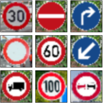
(a) Normal examples

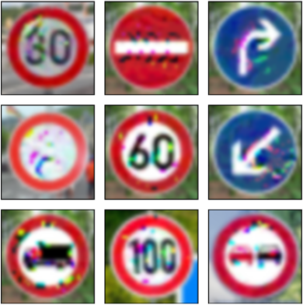
(b) Adversarial examples

Fig. 2: German traffic examples where the adversarial examples are crafted by (Sitawarin et al. 2018).

The classification results are summarized in Table 7.

Attack	ResNet20	${\rm ECNN}^{30}_{0.2}$
None	95.5	97.2
OptProjTran	48.2	79.6

Table 7: Classification accuracy (%) on 392 adversarial GTSRB examples by (Sitawarin et al. 2018).

Impact of Ensemble Diversity

When removing the ensemble diversity from the optimization, the performance decreases significantly. Specifically, using the same shared front network for a fair comparison, we obtain $41.2\%$ accuracy after applying PGD attack using ${\rm ECNN}^{10}_{0.1}$ (cf. Table 2 of supplementary) on CIFAR-10, but we only achieve $17.0\%$ accuracy using ${\rm ECNN}^{10}_{0}$.

Transferability Study

Transferability study is carried out using ${\rm ECNN}^{10}_{\gamma}$ on CIFAR-10, where the $(i,j)$-th entry shown in Fig. 3 is the classification accuracy using the $i$-th network as the substitute model to craft adversarial examples by running PGD at $\epsilon=0.04$ for $200$ iterations and feeding to the $j$-th network. It can be seen that 1) ECNN training yields low transferability among the binary classifiers and 2) having diversity control improves the robustness on individual networks.

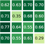
(a) w/ ens. divers., $\gamma=0.1$

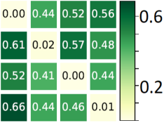
(b) w/o ens. divers., $\gamma=0$

Fig. 3: Adversarial transferability (binary classification accuracy) among binary classifiers in ${\rm ECNN}^{10}_{\gamma}$ on CIFAR-10. The transferability among the first four networks is shown.

Impact of Parameter Sharing

ECNN performs parameter sharing among binary classifiers at both ends of the encoder. Sharing $g^{\{1\}}$ is inspired by the lesson from transfer learning (Yosinski et al. 2014) that features are transferable between neural networks when they are performing similar tasks. Due to Lemma 2, sharing $h$ is to avoid the features extracted from different binary classifiers to be permutations of each other for the same sample $x$. Table 11 shows that performing parameter sharing yields better classification accuracy on normal and adversarial examples than the one with no parameter sharing, i.e., each binary classifier is a composite function $h_{n}\circ g^{\{2\}}_{n}\circ g^{\{1\}}_{n}$. This is mainly because the latter which contains too many parameters overfits the data.

Attack	Para.	w/ para. share	w/o para. share
None	-	85.1	79.2
PGD	$\epsilon=0.04$	71.6	51.1
C&W	$\kappa=1$	80.8	73.2
# params	-	490,497	8,194,590

Table 8: Classification accuracy (%) on adversarial CIFAR-10 examples using ${\rm ECNN}^{30}_{0.1}$ w/ and w/o parameter sharing.

Conclusion

In this paper, we have presented a robust neural network ECNN that is inspired by error-correcting codes and analyzed its properties and proposed a training method that trains the binary classifiers jointly. Designing a code matrix by optimizing both the Hamming distance between rows and VI distance between columns makes ECNN more robust against adversarial examples. We found that performing parameter sharing at two ends of the ECNN’s encoder improves ensemble’s robustness while significantly reducing the number of trainable parameters.

Appendix A Related Work and Adversarial Attacks

In this section we brief more recent works that defend against adversarial examples using ensembles of models (Abbasi and Gagné 2017; Xu, Evans, and Qi 2018; Pang et al. 2019; Verma and Swami 2019; Sen, Ravindran, and Raghunathan 2020) with more details. Then, we discuss common adversarial attacks.

A.1 Ensemble Models

Based on the observation that classifiers can be misled to always decide for a small number of predefined classes through adding perturbations, the work (Abbasi and Gagné 2017) builds an ensemble model that consists of a generalist classifier (which classifies among all $M$ classes) and a collection of specialists (which classify among subsets of the classes). The $m$-th specialist, where $m=0,\ldots,M-1$, classifies among a subset of the original classes, denoted as $\mathcal{U}_{m}$, within which class $m$ is most often confused in adversarial examples. The $(m+M)$-th specialist, where $m=0,\ldots,M-1$, classifies among a subset $\mathcal{U}_{m+M}$ which is complementary to $\mathcal{U}_{m}$, i.e., $\mathcal{U}_{m+M}=\{0,\ldots,M-1\}\setminus\mathcal{U}_{m}$. Altogether there are $2M$ specialists and one generalist. To classify an input, if there exists a class $m$ such that the generalist and the $M$ specialists that can classify $m$ all agree that the input belongs to class $m$, the prediction is made by averaging the outputs of the generalist and the $M$ specialists. Otherwise, at least one classifier has misclassified the input, and the prediction is made by averaging the outputs of all $2M+1$ classifiers in the ensemble.

It has also been observed that the feature input spaces are often unnecessarily large, which leaves an adversary extensive space to generate adversarial examples. The reference (Xu, Evans, and Qi 2018) proposes to “squeeze" out the unnecessary input features. More specifically, (Xu, Evans, and Qi 2018) trains three independent classifiers, respectively on three different versions of an image: the original image, the reduced-color depth version and the spatially smoothed version of the original image. In the testing phase, it compares the softmax probability vectors across these three classifiers’ outputs in terms of $L_{1}$ distance and flags the input as adversarial when the highest pairwise $L_{1}$ distance exceeds a threshold. This method is mainly used for adversarial detection.

Motivated by studies (Pang et al. 2018; Pang, Du, and Zhu 2018) that show theoretically that promoting diversity among learned features of different classes can improve adversarial robustness, the paper (Pang et al. 2019) trains an ensemble of multiple base classifiers with an adaptive diversity promoting (ADP) regularizer that encourages diversity. The ADP regularizer forces the non-maximal prediction probability vectors, i.e., the vector containing all prediction probabilities except the maximal one, learned by different base classifiers to be mutually orthogonal, while keeping the prediction associated with the maximal probability be consistent across all base classifiers.

Inspired by ECOC, which is mostly used with decision trees or shallow neural networks (Dietterich and Bakiri 1994; García-Pedrajas and Fyfe 2008), the authors in (Verma and Swami 2019) design a DNN using error-correcting codes. It splits the binary classifiers into several groups and trains them separately. Each classifier is trained on a different task according to the columns of a predefined code matrix $\mathbf{M}\in\mathbb{R}^{M\times N}$ such as a Hadamard matrix with the aim to increase the diversity of the classifiers so that adversarial examples do not transfer between the classifiers. To generate final predictions, (Verma and Swami 2019) proposes to map logits to the elements of a codeword and assigns probability to class $k$ as

$$p_{\nu}(k)=\frac{\max(\mathbf{m}_{k}^{\intercal}\nu(\mathbf{z}),0)}{\sum_{i=0}^{N-1}\max(\mathbf{m}_{k}^{\intercal}\nu(\mathbf{z}),0)},$$

where $\nu$ can be either logistic function if $\mathbf{M}$ takes values in $\{0,1\}$ or $\tanh$ function if $\mathbf{M}$ takes values in $\{-1,1\}$, and $\mathbf{m}_{k}$ denotes the $k$-th row of $\mathbf{M}$.

Studies (Galloway, Taylor, and Moussa 2017; Rakin et al. 2018) have suggested that quantized models demonstrate higher robustness to adversarial attacks. The work (Sen, Ravindran, and Raghunathan 2020) therefore independently trains multiple models with different levels of precision on their weights and activations, and makes final predictions using majority voting. For example, it uses an ensemble consisting of three models: one full-precision model, i.e., using 32-bit floating point numbers to represent activations and weights, one model trained with 2-bit activation and 4-bit weights, and another model with 2-bit activations and 2-bit weights.

Among the aforementioned ensemble methods, we experimentally compare our proposed ECNN with 1) the ECOC-based DNN proposed in (Verma and Swami 2019) as it shares a similar concept as ours and 2) ADP-based ensemble method proposed in (Pang et al. 2019) as it is the only method among the aforementioned ones that trains the ensemble in an end-to-end fashion. Another reason for choosing these two methods as baseline benchmarks is their reported classification accuracies under adversarial attacks are generally better than the other ensemble methods.

A.2 Overview of Adversarial Attacks

For a normal image-label pair $(x,y)$ and a trained DNN $f_{\theta}$ with $\theta$ being the trainable model parameters, an adversarial attack attempts to find an adversarial example $x^{\prime}$ that remains in the $L_{p}$-ball with radius $\epsilon$ centered at the normal example $x$, i.e., $\|x-x^{\prime}\|_{p}\leq\epsilon$, such that $f_{\theta}(x^{\prime})\neq y$. In what follows, we briefly present some popular adversarial attacks that will be used to verify the robustness of our proposed ECNN.

1. Fast Gradient Sign Method (FGSM) (Goodfellow, Shlens, and Szegedy 2015) perturbs a normal image $x$ in its $L_{\infty}$ neighborhood to obtain

   $$x^{\prime}=x+\epsilon\cdot{\rm sign}\left(\nabla_{x}\mathcal{L}(f_{\theta}(x),y)\right),$$

   where $\mathcal{L}(f_{\theta}(x),y)$ is the cross-entropy loss of classifying $x$ as label $y$, $\epsilon$ is the perturbation magnitude, and the update direction at each pixel is determined by the sign of the gradient evaluated at this pixel. FGSM is a simple yet fast and powerful attack.

2. Basic Iterative Method (BIM) (Kurakin, Goodfellow, and Bengio 2017) iteratively refines the FGSM by taking multiple smaller steps $\alpha$ in the direction of the gradient. The refinement at iteration $i$ takes the following form:

   $$x^{\prime}_{i}=x^{\prime}_{i-1}+{\rm clip}_{\epsilon,x}\left(\alpha\cdot{\rm sign}\left(\nabla_{x}\mathcal{L}(f_{\theta}(x),y)\right)\right),$$

   where $x^{\prime}_{0}=x$ and ${\rm clip}_{\epsilon,x}(x^{\prime})$ performs per-pixel clipping of the image $x^{\prime}$. For example, if a pixel takes value between 0 and 255, ${\rm clip}_{\epsilon,x}(x^{\prime})=\min\left\{255,x+\epsilon,\max\{0,x-\epsilon,x^{\prime}\}\right\}$.

3. Projected Gradient Descent (PGD) (Mądry et al. 2018) has the same generation process as BIM except that PGD starts the gradient descent from a point $x^{\prime}_{0}$ chosen uniformly at random in the $L_{\infty}$-ball of radius $\epsilon$ centered at $x$.

4. Jacobian-based Saliency Map Attack (JSMA) (Papernot et al. 2016a) is a greedy algorithm that adjusts one pixel at a time. Given a target class label $t\neq y$, at each pixel $x_{p,q}$, where $p\in\{1,\ldots,P\}$ and $q\in\{1,\ldots,Q\}$, of a $P\times Q$ image $x$, JSMA computes a saliency map:

   $$S(p,q)=-\alpha_{p,q}\cdot\beta_{p,q}\cdot(\alpha_{p,q}>0)\cdot(\beta_{p,q}<0),$$

   where $\alpha_{p,q}=\frac{\partial Z(x,t)}{\partial x_{p,q}}$, $\beta_{p,q}=\sum_{j\neq t}\frac{\partial Z(x,j)}{\partial x_{p,q}}$, and $Z(x,i)$ denotes the logit associated with label $i$. The logits are the inputs to the softmax function at the output of the DNN classifier. A bigger value of $S(p,q)$ indicates pixel $(p,q)$ has a bigger impact on mis-labeling $x$ as $t$. Let $(p^{*},q^{*})=\underset{p,q}{\operatorname*{arg\,max}}\ S(p,q)$ and set the pixel $x_{p^{*},q^{*}}=\min\left({\rm clip}_{\rm max},x_{p,q}+\theta\right)$, where ${\rm clip}_{\rm max}$ is a pre-defined clipping value. This process repeats until either the misclassification happens or it reaches a pre-defined maximum number of iterations. Note that JSMA is a targeted attack by design. Its untargeted attack variant selects the target class at random.

5. Carlini & Wagner (C&W) (Carlini and Wagner 2017): In this paper, we consider the C&W $L_{2}$ attack only. Let $x^{\prime}=x+\frac{1}{2}(\tanh(\omega)+1)$, where the operations are performed pixel-wise. For a normal example $(x,y)$, C&W finds the attack perturbation by solving the following optimization problem

   $$\underset{\omega}{\min}\ \left\|\frac{1}{2}(\tanh(\omega)+1)-x\right\|^{2}_{2}+c\cdot\ell\left(\frac{1}{2}(\tanh(\omega)+1)\right),$$

   where $\ell(x^{\prime})=\max\left(Z(x^{\prime},y)-\max\{Z(x^{\prime},i):i\neq y\}+\kappa,0\right)$. A large confidence parameter $\kappa$ encourages misclassification.

Appendix B Proof for Lemma 1

1. If $\theta_{n}=\theta$ for all $n=0,\ldots,N-1$, we have ${\mathbf{f}}_{n,x_{k}}=g_{\theta_{n}}(x_{k})=g_{\theta}(x_{k})=\tilde{\mathbf{f}}_{x_{k}}$ for some $\tilde{\mathbf{f}}_{x_{k}}\in\mathbb{R}^{F}$. We then obtain

   $$\bm{\phi}_{n}\left[\tilde{\mathbf{f}}_{x_{0}},\ldots,\tilde{\mathbf{f}}_{x_{K-1}}\right]=\left[z_{n,x_{0}},\cdots,z_{n,x_{K-1}}\right],$$ (11)

   $$~{}\mbox{for all }n=0,\ldots,N-1,$$

   where $z_{n,x_{k}}$ denotes the logits associated with the $k$-th sample and learned by the $n$-th binary classifier.

   We choose $z_{n,x_{k}}$ be such that the loss of 1 can be made arbitrarily small. Here, we consider two loss functions:

   1. The cross entropy loss is used in 2. Let $\bm{\zeta}_{n,x_{k}}$ be $\bm{\zeta}_{n}$ when the input sample is $x_{k}$. Suppose we have

      $$\bm{\zeta}_{n,x_{k}}=\begin{bmatrix}1-\max\left(\varepsilon,\xi\mathbf{M}(y(x_{k}),n)\right)\\ \max\left(\varepsilon,\xi\mathbf{M}(y(x_{k}),n)\right)\end{bmatrix},$$

      where $\varepsilon$ and $\xi$ are positive constants. Then, the loss of 1 can be made arbitrarily small by letting $\varepsilon\to 0$ from above and $\xi\to 1$ from below. Since $\bm{\zeta}_{n,x_{k}}=\left[1-\sigma(z_{n,x_{k}}),\sigma(z_{n,x_{k}})\right]^{\intercal}$, this is equivalent to choosing $z_{n,x_{k}}=\log\left(\frac{\max\left(\varepsilon,\xi\mathbf{M}(y(x_{k}),n)\right)}{1-\max\left(\varepsilon,\xi\mathbf{M}(y(x_{k}),n)\right)}\right)$.

   2. The hinge loss is used in 2. The loss can be made arbitrarily small by choosing $z_{n,x_{k}}$ be such that $\operatorname{sign}\left(2\mathbf{M}(y(x_{k})-1,n)\right)$.

   It now suffices to show that with probability one, there exists a $\bm{\phi}_{n}$ solving 11 for this choice of $\{z_{n,x_{k}}:k=0,\ldots,K-1\}$.

   From 5, $\{\tilde{\mathbf{f}}_{x_{k}}:k=0,\ldots,K-1\}$ are almost surely linearly independent since $K\leq F$ and the joint distribution of $\{\mathbf{n}_{n,x_{k}}:k=0,\ldots,K-1\}$ is absolutely continuous w.r.t. Lebesgue measure. We thus have

   $$\operatorname{rank}\begin{bmatrix}\tilde{\mathbf{f}}_{x_{0}}&\cdots&\tilde{\mathbf{f}}_{x_{K-1}}\\ z_{n,x_{0}}&\cdots&z_{n,x_{K-1}}\end{bmatrix}=\operatorname{rank}\begin{bmatrix}\tilde{\mathbf{f}}_{x_{0}}&\cdots&\tilde{\mathbf{f}}_{x_{K-1}}\end{bmatrix},$$

   i.e., each row in $\left[z_{n,x_{0}},\ldots,z_{n,x_{K-1}}\right]$ belongs to the row space of $\left[\tilde{\mathbf{f}}_{x_{0}},\ldots,\tilde{\mathbf{f}}_{x_{K-1}}\right]$. Hence, there exists a solution $\bm{\phi}_{n}$ to 11 for each $n$. The proof of a is now complete.

2. If $\bm{\phi}_{n}=\bm{\phi}$ for all $n=0,\ldots,N-1$, we have

   $$\bm{\phi}\left[{\mathbf{f}}_{0,x_{0}},\ldots,{\mathbf{f}}_{0,x_{K-1}},\ldots,{\mathbf{f}}_{N-1,x_{0}},\ldots,{\mathbf{f}}_{N-1,x_{K-1}}\right]$$

   $$=\left[z_{0,x_{0}},\ldots,z_{N-1,x_{K-1}}\right].$$ (12)

   Since $NK\leq F$, a similar argument as the proof of a can be applied here to obtain the claim.

3. If $\theta_{n}=\theta$ and $\bm{\phi}_{n}=\bm{\phi}$ for all $n=0,\ldots,N-1$, using the same notations as in the proof of a, we have

   $$\bm{\phi}\left[\tilde{\mathbf{f}}_{x_{0}},\ldots,\tilde{\mathbf{f}}_{x_{K-1}},\ldots,\tilde{\mathbf{f}}_{x_{0}},\ldots,\tilde{\mathbf{f}}_{x_{K-1}}\right]$$

   $$=\left[z_{0,x_{0}},\ldots,z_{N-1,x_{K-1}}\right],$$ (13)

   which implies that $\bm{\phi}\tilde{\mathbf{f}}_{x_{k}}=z_{n,x_{k}}$ holds for all $n=0,\ldots,N-1$. This contradicts the fact that the optimal $z_{n,x_{k}}$, $n=0,\ldots,N-1$, are distinct because the rows in the code matrix $\mathbf{M}$ are designed to be different. The proof of c is now complete.

Appendix C Proof for Lemma 2

Let $z_{n}^{y}=\bm{\phi}_{n}(\mathbf{f}_{n}^{y})$ denote the logits associated with class $y$ for the $n$-th binary classifier.

1. Using the same construction as in the proof of Lemma 1a, we choose $\{z_{n}^{y}\}$ such that the loss of 1 is arbitrarily small. It suffices to show that there exists $\bm{\phi}_{n}$ that satisfy:

   $$\bm{\phi}_{n}\mathbf{S}_{n}\left[{\mathbf{f}}^{0},\ldots,{\mathbf{f}}^{M-1}\right]=\left[z_{n}^{0},\cdots,z_{n}^{M-1}\right],$$ (14)

   for $n=0,\ldots,N-1$. A similar argument as that in the proof of Lemma 1 shows this since $\mathbf{S}_{n}$ is invertible.

2. We show the following equations have no solution $\bm{\phi}$ for almost every $\{\mathbf{f}^{y}\}_{y=0}^{M-1}$:

   $$\bm{\phi}\mathbf{S}_{n}{\mathbf{f}}^{y}=z_{n}^{y},\ n=0,\ldots,N-1.$$ (15)

   Similar to the proof technique used in (Johnson, Šmigoc, and Yang 2014, Theorem 5.2), we define a map

   $$G:\ \mathbb{R}^{FM+F}\to \ \mathbb{R}^{NM}$$

   $$(\bm{\phi}^{\intercal},{\mathbf{f}^{0}},\ldots,{\mathbf{f}^{M-1}})\mapsto$$

   $$\left(\bm{\phi}\mathbf{S}_{0}{\mathbf{f}^{0}},\ldots,\bm{\phi}\mathbf{S}_{0}{\mathbf{f}^{M-1}},\ldots,\bm{\phi}\mathbf{S}_{N-1}\mathbf{f}^{M-1}\right).$$

   It suffices to prove that the image of $G$ has Lebesgue measure $0$ in $\mathbb{R}^{NM}$. By Sard’s theorem, the image of the critical set of $G$ has Lebesgue measure $0$ in $\mathbb{R}^{NM}$, where the critical set of $G$ is the set of points in $\mathbb{R}^{FM+F}$ at which the Jacobian matrix of $G$, denoted as $\mathbf{J}_{G}\in\mathbb{R}^{NM\times(FM+F)}$, has $\operatorname{rank}(\mathbf{J}_{G})<NM$. Therefore, it suffices to show $\operatorname{rank}(\mathbf{J}_{G})<NM$ for all points in $\mathbb{R}^{FM+F}$. We have

   $$\mathbf{J}_{G}=\left[\begin{array}[]{cccc}(\mathbf{f}^{0})^{\intercal}\mathbf{S}_{0}^{\intercal}&\bm{\phi}\mathbf{S}_{0}&\cdots&{\bf 0}\\ \vdots&\vdots&\ddots&\vdots\\ (\mathbf{f}^{M-1})^{\intercal}\mathbf{S}_{0}^{\intercal}&{\bf 0}&\cdots&\bm{\phi}\mathbf{S}_{0}\\ (\mathbf{f}^{0})^{\intercal}\mathbf{S}_{1}^{\intercal}&\bm{\phi}\mathbf{S}_{1}&\cdots&{\bf 0}\\ \vdots&\vdots&\ddots&\vdots\\ (\mathbf{f}^{M-1})^{\intercal}\mathbf{S}_{1}^{\intercal}&{\bf 0}&\cdots&\bm{\phi}\mathbf{S}_{1}\\ \vdots&\vdots&\vdots&\vdots\\ \end{array}\right].$$

   It can be seen

   $$\mathbf{J}_{G}\left[\bm{\phi},-({\mathbf{f}^{0}})^{\intercal},\ldots,-({\mathbf{f}^{M-1}})^{\intercal}\right]^{\intercal}={\bf 0}.$$

   Therefore, the columns of $\mathbf{J}_{G}$ are linearly dependent and thus $\operatorname{rank}(\mathbf{J}_{G})<FM+F\leq NM$ holds for every point in $\mathbb{R}^{FM+F}$. The proof is now complete if we note that there are only finitely many permutation matrices.

Appendix D Proof for Lemma 3

Consider the model where we set the feature vector $\mathbf{f}_{n,x}$ to be $\mathbf{f}^{y(x)}_{n}$ for all $n$ and $x$. Using a similar argument as in the proof of Lemma 1b, it can be shown that there exists $\{\bm{\phi}_{n}=\bm{\phi}\}_{n=0}^{N-1}$ such that the loss of 1 is sufficiently small so that $z^{y(x_{k})}_{n}(\mathbf{M}(y(x_{k}),n))>z^{y(x_{k})}_{n}(1-\mathbf{M}(y(x_{k}),n))$, for all $k=0,\ldots,K-1$, where $z^{y(x_{k})}_{n}=\bm{\phi}(\mathbf{f}^{y(x_{k})}_{n})$. For this choice of $\bm{\phi}_{n}=\bm{\phi}$ now applied to the model in the lemma, we have for each $n$ and $x_{k}$,

$$z_{n,x_{k}} =\bm{\phi}\mathbf{f}_{n,x_{k}}$$

$$=\bm{\phi}(\mathbf{f}^{y(x_{k})}_{n}+\mathbf{n}_{n,x_{k}})$$

$$=z^{y(x_{k})}_{n}+\bm{\phi}\mathbf{n}_{n,x_{k}},$$

so that

$$\operatorname{sign}\left(z_{n,x_{k}}(0)-z_{n,x_{k}}(1)\right)=\operatorname{sign}\left(z^{y(x_{k})}_{n}(0)-z^{y(x_{k})}_{n}(1)\right)$$

if $\left|\mathbf{n}_{n,x_{k}}^{\intercal}\left(\bm{\phi}_{0}-\bm{\phi}_{1}\right)\right|<\left|z^{y(x_{k})}_{n}(0)-z^{y(x_{k})}_{n}(1)\right|$, where $\bm{\phi}=\left[\bm{\phi}_{0}^{\intercal},\bm{\phi}_{1}^{\intercal}\right]^{\intercal}$. From the Cauchy-Schwarz inequality, $\left|\mathbf{n}_{n,x_{k}}^{\intercal}\left(\bm{\phi}_{0}-\bm{\phi}_{1}\right)\right|\leq\|\mathbf{n}_{n,x_{k}}\|_{2}\|\bm{\phi}_{0}-\bm{\phi}_{1}\|_{2}$ and thus zero classification error for the $n$-th binary classifier is achievable if $\|\mathbf{n}_{n,x_{k}}\|_{2}$ is sufficiently small. The proof is now complete.

Appendix E Proof for Lemma 4

Suppose cross entropy loss is used in 2. The optimization in Joint Optimization w.r.t. $\bm{\zeta}_{n,x_{k}}$ becomes

$$\min_{\bm{\zeta}_{n,x_{k}}} ~{}\frac{1}{NK}\sum_{k=0}^{K-1}\sum_{n=0}^{N-1}-\left({\bf 1}_{y_{n}(x_{k})}-\gamma\bm{\zeta}_{n,x_{k}}\right)^{\intercal}\log\left(\bm{\zeta}_{n,x_{k}}\right)$$ (16)

$${\rm s.t.} ~{}\sum_{i=0}^{1}\bm{\zeta}_{n,x_{k}}(i)=1,$$

where $\gamma>0$.

The Lagrangian of 16 is

$$L= \frac{1}{NK}\sum_{k=0}^{K-1}\sum_{n=0}^{N-1}\left(-{\bf 1}_{y_{n}(x_{k})}^{\intercal}\log\left(\bm{\zeta}_{n,x_{k}}\right)+\gamma\bm{\zeta}_{n,x_{k}}^{\intercal}\log(\bm{\zeta}_{n,x_{k}})\right)$$

$$-\sum_{k=0}^{K-1}\sum_{n=0}^{N-1}a_{n,k}\left(1-\sum_{i}\bm{\zeta}_{n,x_{k}}(i)\right),$$

where $a_{n,k}\geq 0,\text{ for all }n,k$. Differentiating $L$ w.r.t. $\bm{\zeta}_{n,x_{k}}(i)$ and equating to zero yields

$$\frac{\partial L}{\partial\bm{\zeta}_{n,x_{k}}(y_{n}(x_{k}))}= -\frac{1}{\bm{\zeta}_{n,x_{k}}(y_{n}(x_{k}))}+\gamma\left(\log(\bm{\zeta}_{n,x_{k}}(y_{n}(x_{k})))+1\right)$$

$$+a_{n,k}=0,$$

$$\frac{\partial L}{\partial\bm{\zeta}_{n,x_{k}}(i)}= \gamma\left(\log(1-\bm{\zeta}_{n,x_{k}}(y_{n}(x_{k})))+1\right)+a_{n,k}=0,$$

$$\text{ for all }i\neq y_{n}(x_{k}).$$

Equating the above two equations, we have $\gamma\log\frac{\bm{\zeta}_{n,x_{k}}(y_{n}(x_{k}))}{1-\bm{\zeta}_{n,x_{k}}(y_{n}(x_{k}))}=\frac{1}{\bm{\zeta}_{n,x_{k}}(y_{n}(x_{k}))}$. This completes the proof.

Appendix F Proof for Lemma 5

We can easily see that $s(k,\ell)=\frac{1}{M}$ if $\ell\in C^{k}$; $s(k,\ell)=0$ otherwise. Then, $I(\mathbf{y},\mathbf{c})$ in 10 can be rewritten as

$$I(\mathbf{y},\mathbf{c}) =\sum_{k=0}^{q-1}\frac{\left|C^{k}\right|}{M}\log\frac{\frac{1}{M}}{\frac{\left|C^{k}\right|}{M}\frac{1}{M}}$$

$$=\sum_{k=0}^{q-1}\frac{\left|C^{k}\right|}{M}\log\frac{M}{\left|C^{k}\right|}.$$

The maximum of $I(\mathbf{y},\mathbf{c})$ is achieved when $\left|C^{k}\right|=M/q,\text{ for all }k$, i.e., $\max I(\mathbf{y},\mathbf{c})=\log q$, which increases with $q$. The proof is complete.

Appendix G Training $q$-ary ECNN

We introduce a method to implement a general $q$-ary ECNN, where $q\geq 2$.

G.1 Encoder

The logits, i.e., the encoder’s outputs, in Fig. 1 becomes $\mathbf{z}_{n}=h_{n}({\mathbf{f}}_{n})\in\mathbb{R}^{q}$. Using a multi-class hinge loss (Carlini and Wagner 2017), the encoder can be formulated as an optimization problem:

$$\min_{\{\theta_{n},\bm{\phi}_{n}\}_{n=0}^{N-1}} \ \frac{1}{NK}\sum_{k=0}^{K-1}\sum_{n=0}^{N-1}\max\left(\max\{\mathbf{z}_{n,x_{k}}(i):i\neq\mathbf{M}(y(x_{k}),n)\}\right.$$

$$\left.-\mathbf{z}_{n,x_{k}}(\mathbf{M}(y(x_{k}),n))+\kappa,0\right)$$ (17)

$${\rm s.t.} ~{}\text{for $k=0,\ldots,K-1$ and $n=0,\ldots,N-1$},$$

$$\ z_{n,x_{k}}=\bm{\phi}_{n}g_{\theta_{n}}(x_{k}),$$

where $\mathbf{M}$ denotes a $q$-ary code matrix and $\kappa$ is the confidence level which is configurable. Finally, the logits $\mathbf{z}_{n}$ are concatenated into $\mathbf{z}=\left[\mathbf{z}_{0}^{\intercal},\ldots,\mathbf{z}_{N-1}^{\intercal}\right]^{\intercal}\in\mathbb{R}^{qN}$, which is the input to the decoder in ECNN.

G.2 Decoder

The decoder maps the logits $\mathbf{z}$ to the prediction probabilities $\mathbf{p}={\sigma}\left(\mathbf{M}\nu(\mathbf{z})\right)\in\mathbb{R}^{M}$, where $\sigma(\cdot)$ denotes the softmax function and $\nu(\cdot)$ denotes the logistic function.

G.3 Joint Optimization

The joint optimization for a $q$-ary ECNN is as follows

$$\min_{\{\theta_{n}\}_{n=0}^{N-1},\bm{\phi}} ~{}\frac{1}{NK}\sum_{k=0}^{K-1}\sum_{n=0}^{N-1}\max\left(\max\{\mathbf{z}_{n,x_{k}}(i):i\neq\mathbf{M}(y(x_{k}),n)\}\right.$$

$$\ \left.-\mathbf{z}_{n,x_{k}}(\mathbf{M}(y(x_{k}),n))+\kappa,0\right)-\gamma\bm{\zeta}_{n,x_{k}}\log\left(\bm{\zeta}_{n,x_{k}}\right),$$ (18)

$${\rm s.t.} ~{}\text{for }n=0,\ldots,N-1,\ k=0,\ldots,K-1,$$

$$~{}\mathbf{z}_{n,x_{k}}=\bm{\phi}g_{\theta_{n}}(x_{k}),\ \bm{\zeta}_{n,x_{k}}=\sigma(\mathbf{z}_{n,x_{k}}),$$

where $\gamma\geq 0$ is a configurable weight.

Appendix H Further Experiments

Denote $\text{Res}_{i,j},i,j\in\{0,1,2\}$ as the $j$-th residual unit in the $i$-th stack. Table 9 shows how the functions $g^{\{1\}}$ and $g^{\{2\}}_{n}$ are constructed using the residual units in ResNet20.

Table 9: The neural networks for $h,g^{\{2\}}_{n},g^{\{1\}}$.

$g^{\{1\}}$	$g^{\{2\}}_{n}$	$h$
$\text{Res}_{0,0}$	$\text{Res}_{2,2}$	Dense(1, Linear)
$\cdots$	Dense(32, ReLu)
$\text{Res}_{2,1}$

The ECNNs used to get all our experimental results do not use batch norms (BNs), however, we found that adding BNs to ECNN will slightly improve ECNN’s classification accuracy on both normal and adversarial examples.

The PGD attack implemented in Table 3 and Table 4 uses a hinge loss proposed in (Carlini and Wagner 2017). The optimal perturbation $\delta^{*}$ is thus found by solving

$$\min_{\delta}\ -\max\left(\mathbf{s}_{x+\delta}(y(x+\delta))-\max\{\mathbf{s}_{x+\delta}(i):i\neq y(x)\}+c,0\right),$$

where $\mathbf{s}$ denotes the logits from the decoder and $c=50$.

H.1 Number of Ensemble Members in ECNN

For a $10$-label classification problem, representing labels with unique codewords requires $N\geq 4$. In this experiment, we independently generate five code matrices for $N=10,15,20,25,30$, respectively, and use them to construct five ECNNs. The settings of adversarial attacks are the same as Table 4. Table 10 shows that when $N$ is small, ECNN has inferior performances on adversarial examples. One possible reason is that we use a dense layer with the same feature dimension $F=32$ for all $N$ in our experiments. From Lemma 2, we know that when $F\gg N$, it may happen that the features $\mathbf{f}^{y(x)}_{n}$ for different binary classifiers $n=0,\ldots,N-1$ are permutations of each other for the same sample $x$. Adversarial attacks on a particular binary classifier can then translate to the other classifiers.

Table 10: Classification accuracy (%) on adversarial CIFAR10 examples using ${\rm ECNN}^{N}_{0.1}$ where $N=10,15,20,25,30$.

Attack	Para.	$N=10$	$N=15$	$N=20$	$N=25$	$N=30$
None	-	84.6	85.5	85.1	85.5	85.1
PGD	$\epsilon=0.04$	41.2	49.9	50.2	48.5	71.6
C&W	-	72.0	71.4	74.1	71.8	80.8
# of params	-	294,977	343,857	392,737	441,617	490,497

H.2 Parameter Sharing

As shown in Table 9, ECNN performs parameter sharing among binary classifiers at both ends of the encoder. Sharing $g^{\{1\}}$ is inspired by the idea from transfer learning (Yosinski et al. 2014) which says the features are transferable between neural networks when they are performing similar tasks. Due to Lemma 2, sharing $h$ is to avoid the features extracted from different binary classifiers to be permutations of each other for the same sample $x$.

Define $|g^{\{1\}}|$ as the number of trainable parameters in $g^{\{1\}}$ and define $|g^{\{2\}}_{n}|,n=0,\ldots,N-1$ and $|h|$ analogously. The total number of trainable parameters in ECNN can be computed as $|g^{\{1\}}|+\sum_{n=0}^{N-1}|g^{\{2\}}_{n}|+|h|$. If $|g^{\{1\}}|+|h|$ is much larger than any $|g^{\{2\}}_{n}|$, the growth of the total number of parameters in ECNN when $N$ increases will be very slow. Table 11 shows that performing parameter sharing yields better classification accuracy on normal and adversarial examples than the one with no parameter sharing, i.e., each binary classifier is a composite function $h_{n}\circ g^{\{2\}}_{n}\circ g^{\{1\}}_{n}$. This is mainly because the latter which contains too many parameters overfits the data.

Table 11: Classification accuracy (%) on adversarial CIFAR10 examples using ${\rm ECNN}^{30}_{0.1}$ with and without parameter sharing.

Attack	Para.	w/ para. share	w/o para. share
None	-	85.1	79.2
PGD	$\epsilon=0.04$	71.6	51.1
C&W	-	80.8	73.2
# of params	-	490,497	8,194,590

H.3 Code Matrix

In this experiment, we investigate the impact of code matrix design on ECNN’s performance. To highlight the benefit of optimizing both row and column distances, we construct a code matrix $\mathbf{M}^{\prime}=\left[\mathbf{M}_{a},\mathds{1}-\mathbf{M}_{a}\right]$ of size $10\times 30$ where $\mathbf{M}_{a}$ is of size $10\times 15$ and is the first $15$ columns extracted from the code matrix generated by optimizing 9. $\mathbf{M}^{\prime}$’s minimum VI distance between columns is 0 while its minimum Hamming distance between rows remains large. As shown in Table 12, the ECNN trained on $\mathbf{M}^{\prime}$ has worse testing accuracy on adversarial examples so that optimizing both row and column distance is advised in practice.

Table 12: Classification accuracy (%) on adversarial CIFAR10 examples with a codematrix whose minimum VI distance between columns is 0.

Attack	Para.	$\mathbf{M}$	$\mathbf{M}^{\prime}$
None	-	85.1	84.0
PGD	$\epsilon=0.04$	71.6	31.1
C&W	-	80.8	56.0

H.4 Fine-tuning C&W Attack and Logits Level Attack Using PGD

Reference (Zhang, Tondi, and Barni 2020) reports that ECOC-based DNN, i.e., TanhEns16, proposed in (Verma and Swami 2019) is vulnerable to the white-box attacks when they are carried out properly. So, we test our ECNN’s robustness under the fine-tuning C&W attack suggested in (Zhang, Tondi, and Barni 2020) and PGD attack which works on the logits level from the encoder, i.e., $\mathbf{z}_{n},n=0,\ldots,N-1$. For PGD attack, the hinge loss (Carlini and Wagner 2017) is used as the attack loss function. We use $q$-ary ECNN as the training model. Table 13 shows that both attacks are not very successful to fool $q$-ary ECNN with $q=2,3,4$. One reason could be that we use the multi-class hinge loss proposed in (Carlini and Wagner 2017) as the loss function during training which counteracts these two attacks as they are also using this hinge loss as their attack loss functions. Moreover, we suspect that the attack parameters and/or loss functions for these two attacks are not optimized. So, as a future work, we will test ECNN using more effective attacks.

Table 13: Classification accuracy (%) on adversarial CIFAR10 examples crafted by the fine-tuning C&W attack suggested in (Zhang, Tondi, and Barni 2020) and PGD attack working on logits $\mathbf{z}_{n},n=0,\ldots,N-1$ at the encoder’s outputs using $q$-ary ${\rm ECNN}^{30}_{0.1}$ where $q=2,3,4$. We set the confidence level $\kappa=1$ in Section G.3.

Attack	Para.	$q=2$	$q=3$	$q=4$
None	-	85.0	84.4	84.3
Fine-tuning C&W (Zhang, Tondi, and Barni 2020)	initial constant$=0.1$
	max iteration $=2000$	81.5	82.5	82.0
	confidence $\kappa=0$
PGD on logits $\mathbf{z}_{n}$	$\epsilon=0.04$	79.1	80.2	80.4
# of params	-	490,530	490,563	490,596

References

- Abbasi and Gagné (2017) Abbasi, M.; and Gagné, C. 2017. Robustness to Adversarial Examples through an Ensemble of Specialists. In Proc. Int. Conf. Learning Representations Workshop.
- Andor et al. (2016) Andor, D.; Alberti, C.; Weiss, D.; Severyn, A.; Presta, A.; Ganchev, K.; Petrov, S.; and Collins, M. 2016. Globally Normalized Transition-Based Neural Networks. In Proc. Annu. Meeting Assoc, Comput. Linguistics.
- Carlini and Wagner (2017) Carlini, N.; and Wagner, D. 2017. Towards evaluating the robustness of neural networks. In Proc. IEEE Symp. Security and Privacy.
- Dietterich and Bakiri (1994) Dietterich, T. G.; and Bakiri, G. 1994. Solving multiclass learning problems via error correcting output codes. J. Artificial Intell. Res. 2(1): 263–286.
- Galloway, Taylor, and Moussa (2017) Galloway, A.; Taylor, G. W.; and Moussa, M. 2017. Attacking Binarized Neural Networks .
- Gamal et al. (1987) Gamal, A.; Hemachandra, L.; Shperling, I.; and Wei, V. 1987. Using simulated annealing to design good codes. IEEE Trans. Inf. Theory 33(1): 116–123.
- García-Pedrajas and Fyfe (2008) García-Pedrajas, N.; and Fyfe, C. 2008. Evolving output codes for multiclass problems. IEEE Trans. Evol. Comput. 12(1): 93–106.
- Goodfellow, Shlens, and Szegedy (2015) Goodfellow, I. J.; Shlens, J.; and Szegedy, C. 2015. Explaining and harnessing adversarial examples. In Proc. Int. Conf. Learning Representations.
- He et al. (2016) He, K.; Zhang, X.; Ren, S.; and Sun, J. 2016. Deep residual learning for image recognition. In Proc. Conf. Comput. Vision Pattern Recognition.
- Hendrycks and Gimpel (2017) Hendrycks, D.; and Gimpel, K. 2017. A Baseline for Detecting Misclassified and Out-of-Distribution Examples in Neural Networks. In Proc. Int. Conf. Learning Representations.
- Hinton et al. (2012) Hinton, G.; Deng, L.; Yu, D.; Dahl, G. E.; Mohamed, A.; Jaitly, N.; Senior, A.; Vanhoucke, V.; Nguyen, P.; Sainath, T. N.; and Kingsbury, B. 2012. Deep Neural Networks for Acoustic Modeling in Speech Recognition: The Shared Views of Four Research Groups. IEEE Signal Process. Mag. 29(6): 82–97.
- Johnson, Šmigoc, and Yang (2014) Johnson, C. R.; Šmigoc, H.; and Yang, D. 2014. Solution theory for systems of bilinear equations. Linear and Multilinear Algebra 62(12): 1553–1566.
- Kirkpatrick, Gelatt, and Vecchi (1983) Kirkpatrick, S.; Gelatt, C. D.; and Vecchi, M. P. 1983. Optimization by simulated annealing. Science 220(4598): 671–680.
- Krizhevsky and Hinton (2009) Krizhevsky, A.; and Hinton, G. 2009. Learning multiple layers of features from tiny images. Master’s thesis, Department of Computer Science, University of Toronto .
- Krizhevsky, Sutskever, and Hinton (2012) Krizhevsky, A.; Sutskever, I.; and Hinton, G. E. 2012. ImageNet classification with deep convolutional neural networks. In Proc. Advances Neural Inf. Process. Syst.
- Kurakin, Goodfellow, and Bengio (2017) Kurakin, A.; Goodfellow, I. J.; and Bengio, S. 2017. Adversarial examples in the physical world. In Proc. Int. Conf. Learning Representations.
- LeCun et al. (1998) LeCun, Y.; Bottou, L.; Bengio, Y.; and Haffner, P. 1998. Gradient-based learning applied to document recognition. Proceedings of the IEEE 86(11): 2278–2324.
- LeCun, Corte, and Burges (2010) LeCun, Y.; Corte, C.; and Burges, C. 2010. MNIST handwritten digit database. ATT Labs [Online]. Available: http://yann.lecun.com/exdb/mnist 2. (Last accessed: Dec 1, 2020).
- Meilă (2003) Meilă, M. 2003. Comparing clusterings by the variation of information. In Proc. Annu Conf. Learning Theory.
- Meng and Chen (2017) Meng, D.; and Chen, H. 2017. Magnet: a two-pronged defense against adversarial examples. In Proc. SIGSAC Conf. Comput. Commun. Security.
- Mądry et al. (2018) Mądry, A.; Makelov, A.; Schmidt, L.; Tsipras, D.; and Vladu, A. 2018. Towards deep learning models resistant to adversarial attacks. In Proc. Int. Conf. Learning Representations.
- Pang et al. (2018) Pang, T.; Du, C.; Dong, Y.; and Zhu, J. 2018. Towards Robust Detection of Adversarial Examples. In Proc. Advances Neural Inf. Process. Syst.
- Pang, Du, and Zhu (2018) Pang, T.; Du, C.; and Zhu, J. 2018. Max-Mahalanobis Linear Discriminant Analysis Networks. In Proc. Int. Conf. Mach. Learning.
- Pang et al. (2019) Pang, T.; Xu, K.; Du, C.; Chen, N.; and Zhu, J. 2019. Improving adversarial robustness via promoting ensemble diversity. In Proc. Int. Conf. Mach. Learning.
- Papernot et al. (2016a) Papernot, N.; McDaniel, P.; Jha, S.; Fredrikson, M.; Celik, Z. B.; and Swami, A. 2016a. The limitations of deep learning in adversarial settings. In Proc. IEEE Eur. Symp. Security Privacy.
- Papernot et al. (2016b) Papernot, N.; McDaniel, P.; Wu, X.; Jha, S.; and Swami, A. 2016b. Distillation as a defense to adversarial perturbations against deep neural networks. In Proc. IEEE Symp. Security and Privacy.
- Pujol, Radeva, and Vitria (2006) Pujol, O.; Radeva, P.; and Vitria, J. 2006. Discriminant ECOC: A heuristic method for application dependent design of error correcting output codes. IEEE Trans. Pattern Anal. Mach. Intell. 28(6): 1007–1012.
- Rakin et al. (2018) Rakin, A. S.; Yi, J.; Gong, B.; and Fan, D. 2018. Defend Deep Neural Networks Against Adversarial Examples via Fixed andDynamic Quantized Activation Functions .
- Samangouei, Kabkab, and Chellappa (2018) Samangouei, P.; Kabkab, M.; and Chellappa, R. 2018. Defense-GAN: protecting classifiers against adversarial attacks using generative models. In Proc. Int. Conf. Learning Representations.
- Sen, Ravindran, and Raghunathan (2020) Sen, S.; Ravindran, B.; and Raghunathan, A. 2020. EMPIR: Ensembles of Mixed Precision Deep Networks for Increased Robustness Against Adversarial Attacks. In Proc. Int. Conf. Learning Representations.
- Sermanet and LeCun (2011) Sermanet, P.; and LeCun, Y. 2011. Traffic sign recognition with multi-scale Convolutional Networks. In Proc. Int. Joint Conf. Neural Networks, 2809–2813.
- Sitawarin et al. (2018) Sitawarin, C.; Bhagoji, A.; Mosenia, A.; Mittal, P.; and Chiang, M. 2018. Rogue Signs: Deceiving Traffic Sign Recognition with Malicious Ads and Logos. In Deep Learning and Security Workshop.
- Stallkamp et al. (2012) Stallkamp, J.; Schlipsing, M.; Salmen, J.; and Igel, C. 2012. Man vs. computer: Benchmarking machine learning algorithms for traffic sign recognition. Neural Networks 32(1): 323–332.
- Szegedy et al. (2016) Szegedy, C.; Vanhoucke, V.; Ioffe, S.; Shlens, J.; and Wojna, Z. 2016. Rethinking the Inception Architecture for Computer Vision. In Proc. Conf. Comput. Vision Pattern Recognition.
- Szegedy et al. (2013) Szegedy, C.; Zaremba, W.; Sutskever, I.; Bruna, J.; Erhan, D.; Goodfellow, I.; and Fergus, R. 2013. Intriguing properties of neural networks. In Proc. Int. Conf. Learning Representations.
- Tramèr et al. (2020) Tramèr, F.; Carlini, N.; Brendel, W.; and Madry, A. 2020. On Adaptive Attacks to Adversarial Example Defenses. ArXiv abs/2002.08347.
- Verma and Swami (2019) Verma, G.; and Swami, A. 2019. Error correcting output codes improve probability estimation and adversarial robustness of deep neural networks. In Proc. Advances Neural Inf. Process. Syst.
- Xu, Evans, and Qi (2018) Xu, W.; Evans, D.; and Qi, Y. 2018. Feature Squeezing: Detecting Adversarial Examples in Deep Neural Networks. In Proc. Annu. Network and Distributed System Security Symp.
- Yosinski et al. (2014) Yosinski, J.; Clune, J.; Bengio, Y.; and Lipson, H. 2014. How transferable are features in deep neural networks? In Proc. Advances Neural Inf. Process. Syst.
- Zhang, Tondi, and Barni (2020) Zhang, B.; Tondi, B.; and Barni, M. 2020. On the adversarial robustness of DNNs based on error correcting output codes .