Correction Filter for Single Image Super-Resolution:
Robustifying Off-the-Shelf Deep Super-Resolvers

Abstract

The single image super-resolution task is one of the most examined inverse problems in the past decade. In the recent years, Deep Neural Networks (DNNs) have shown superior performance over alternative methods when the acquisition process uses a fixed known downscaling kernel—typically a bicubic kernel. However, several recent works have shown that in practical scenarios, where the test data mismatch the training data (e.g. when the downscaling kernel is not the bicubic kernel or is not available at training), the leading DNN methods suffer from a huge performance drop. Inspired by the literature on generalized sampling, in this work we propose a method for improving the performance of DNNs that have been trained with a fixed kernel on observations acquired by other kernels. For a known kernel, we design a closed-form correction filter that modifies the low-resolution image to match one which is obtained by another kernel (e.g. bicubic), and thus improves the results of existing pre-trained DNNs. For an unknown kernel, we extend this idea and propose an algorithm for blind estimation of the required correction filter. We show that our approach outperforms other super-resolution methods, which are designed for general downscaling kernels.

(a) Original image (cropped)

(b) LR image

(c) Bicubic upsampling

(d) SRMD [39]

(e) ZSSR [27]

(f) ProSR [35]

(g) RCAN [41]

(h) DBPN [15]

(i) ProSR with our correction

(j) RCAN with our correction

(k) DBPN with our correction

Figure 1: Non-blind super-resolution of image 223061 from BSD100, for scale factor 4 and Gaussian downscaling kernel with std $4.5/\sqrt{2}$. Our correction filter significantly improves the performance of DNNs trained on another SR kernel.

1 Introduction

The task of Single Image Super-Resolution (SISR) is one of the most examined inverse problems in the past decade [11, 13, 37, 8]. In this problem, the goal is to reconstruct a latent high-resolution (HR) image from its low-resolution (LR) version obtained by an acquisition process that includes low-pass filtering and sub-sampling. In the recent years, along with the developments in deep learning, many SISR methods that are based on Deep Neural Networks (DNNs) have been proposed [7, 17, 21, 20, 41, 35, 15].

Typically, the performance of SISR approaches is evaluated on test sets with a fixed known acquisition process, e.g. a bicubic downscaling kernel. This evaluation methodology allows to prepare large training data, which are based on ground truth HR images and their LR counterparts synthetically obtained through the known observation model. DNNs, which have been exhaustively trained on such training data, clearly outperform other alternative algorithms, e.g. methods that are based on hand-crafted prior models such as sparsity or non-local similarity [8, 13, 37].

Recently, several works have shown that in practical scenarios where the test data mismatch the training data, the leading DNN methods suffer from a huge performance drop [38, 27, 30]. Such scenarios include a downscaling kernel which is not the bicubic kernel and is not available at the training phase. A primary example is an unknown kernel that needs to be estimated from the LR image at test time.

Several recent SISR approaches have proposed different strategies for enjoying the advantages of deep learning while mitigating the restriction of DNNs to the fixed kernel assumption made in the training phase. These strategies include: modifying the training phase such that it covers a predefined set of downscaling kernels [39, 14]; using DNNs to capture only a natural-image prior which is decoupled from the SISR task [38, 5]; or completely avoid any offline training and instead train a CNN super-resolver from scratch at test time [32, 27].

Contribution. In this work we take a different strategy, inspired by the generalized sampling literature [9, 33], for handling LR images obtained by arbitrary downscaling kernels. Instead of completely ignoring the state-of-the-art DNNs that have been trained for the bicubic model, as done by other prior works, we propose a method that transforms the LR image to match one which is obtained by the bicubic kernel. The modified LR can then be inserted into existing leading super-resolvers, such as DBPN [15], RCAN [41], and proSR [35], thus, improving their performance significantly on kernels they have not been trained on. The proposed transformation is performed using a correction filter, which has a closed-form expression when the true (non-bicubic) kernel is given.

In the ”blind” setting, where the kernel is unknown, we extend our approach and propose an algorithm that estimates the required correction. The proposed approach outperforms other super-resolution methods in various practical scenarios. See example results in Figure 1 for the non-blind setting.

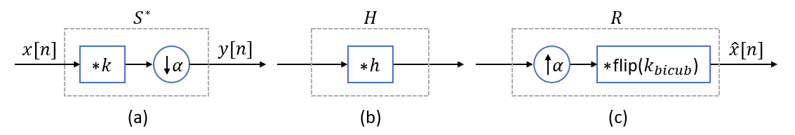
Figure 2: Downsampling, correction, and upsampling operators for single image super-resolution: (a) Downsampling operator composed of convolution with a kernel $\mathbf{k}$ and sub-sampling by factor of $\alpha$; (b) Correction operator composed of convolution with a correction filter $\mathbf{h}$; (c) Upsampling operator composed of up-sampling by factor of $\alpha$ and convolution with a (flipped) kernel $\mathbf{k}_{bicub}$. In our approach, $\mathcal{H}$ is computed for $\mathcal{S}^{*}$ and $\mathcal{R}$, but then we replace $\mathcal{R}$ with a pre-trained DNN super-resolver.

2 Related Work

In the past five years many works have employed DNNs for the SISR task, showing a great advance in performance with respect to the reconstruction error [7, 15, 17, 21, 35, 41] and the perceptual quality [4, 20, 25, 34]. However, one main disadvantage of DNN-based SISR methods is their sensitivity to the LR image formation model. A network performance tends to drop significantly if it has been trained for one acquisition model and then been tested on another [27, 30, 38].

Recently, different SISR strategies has been proposed with the goal of enjoying the advantages of deep learning while mitigating the restriction of DNNs to the fixed kernel assumption made in the training phase. One approach trains a CNN super-resolver that gets as inputs both the LR image and the degradation model, and assumes that the downscaling kernels belong to a certain set of Gaussian filters [14, 39]. Another approach builds on the structural prior of CNNs, which promotes signals with spatially recurring patterns (e.g. natural images) and thus allows to train a super-resolver CNN from scratch at test time [27, 32]. Another line of work recovers the latent HR image by minimizing a cost function that is composed of a fidelity term (e.g. least squares or back-projection [31]) and a prior term, where only the latter is handled by a pre-trained CNN denoiser or GAN [38, 29, 5, 40]. Recently, the two last approaches have been incorporated by applying image-adaptation to denoisers [30] and GANs [1]. In all these methods the downscaling kernel is given as an input. In a blind setting (where the kernel is unknown) it is still possible to apply these methods after an initial kernel estimation phase.

Our approach is inspired by the literature on generalized sampling [6, 33, 9], which generalizes the classical Whittaker–Nyquist–Kotelnikov–Shannon sampling theorem [36, 23, 19, 26], which considers signals that are band-limited in the frequency domain and sinc interpolations. The generalized theory provides a framework and conditions under which a signal that is sampled by a certain basis can be reconstructed by a different basis. In this framework, the sampled signal is reconstructed using a linear operator that can be decoupled into two phases, the first applies a digital correction filter and the second includes processing with a reconstruction kernel. The role of the correction filter is to transform the sampling coefficients, associated with the sampling kernel, to coefficients which fit the reconstruction kernel.

Several works have used the correction filter approach for image processing [10, 12, 24]. These works typically propose linear interpolation methods, i.e. the correction filter is followed by a linear reconstruction operation, and do not use a strong natural-image prior. As a result, the recovery of fine details is lacking.

In this work, we plan to use (very) non-linear reconstruction methods, namely—DNNs, whose training is difficult, computationally expensive, storage demanding, and cannot be done when the observation model is not known in advance. To tackle these difficulties, we revive the correction filter approach and show how it can be used with deep super-resolvers which have been already trained.

The required correction filter depends on the kernel which is used for sampling. Therefore, in the blind setting, it needs to be estimated from the LR image. To this end, we propose an iterative optimization algorithm for estimating the correction filter. In general, only a few works have considered the blind SISR setting and developed kernel estimation methods [28, 22, 14, 3].

Finally, we would like to highlight major differences between this paper and the work in [14], whose ”kernel correction” approach may be misunderstood as our ”correction filter”. In [14], three different DNNs (super-resolver, kernel estimator, and kernel corrector) are offline trained under the assumption that the downscaling kernel belongs to a certain family of Gaussian filters (similarly to [39]), and the CNN super-resolver gets the estimated kernel as an input. So, the first major difference is that contrary to our approach, no pre-trained existing DNN methods (other than SRMD [39]) can be used in [14]. Secondly, their approach is restricted by the offline training assumptions to very certain type of downscaling kernels, contrary to our approach. Thirdly, the concepts of these works are very different: The (iterative) correction in [14] modifies the estimated downscaling kernel, while our correction filter modifies the LR image.

3 The Proposed Method

The single image super resolution (SISR) acquisition model, can be formulated as

$$\mathbf{y}=(\mathbf{x}\ast\mathbf{k})\downarrow_{\alpha},$$ (1)

where $\mathbf{x}\in\mathbb{R}^{n}$ represents the latent HR image, $\mathbf{y}\in\mathbb{R}^{m}$ represents the observed LR image, $\mathbf{k}\in\mathbb{R}^{d}$ $(d\ll n)$ is the (anti-aliasing) blur kernel, $\ast$ denotes the linear convolution operator, and $\downarrow_{\alpha}$ denotes sub-sampling operator with stride of $\alpha$. Under the common fashion of dropping the edges of $\mathbf{x}\ast\mathbf{k}$, such that it is in $\mathbb{R}^{n}$, we have that $m=\left\lceil n/\alpha\right\rceil$.

Note that Equation (1) can be written in a more elegant way as

$$\mathbf{y}=\mathcal{S}^{*}\mathbf{x},$$ (2)

where $\mathcal{S}^{*}:\mathbb{R}^{n}\rightarrow\mathbb{R}^{m}$ is a linear operator that encapsulates the entire downsampling operation, i.e. $\mathcal{S}^{*}$ is a composition of blurring followed by sub-sampling. The downsampling operator $\mathcal{S}^{*}$ is presented in Figure 2(a).

Most SISR deep learning methods, e.g. [7, 17, 21, 20, 41, 35, 15], assume that the observations are obtained using the bicubic kernel. Let us denote by $\mathcal{R}^{*}$ the associated downsampling operator (essentially, $\mathcal{R}^{*}$ coincides with the previously defined $\mathcal{S}^{*}$ if $\mathbf{k}$ is the bicubic kernel $\mathbf{k}_{bicub}$). The core idea of our approach is to modify the observations $\mathbf{y}=\mathcal{S}^{*}\mathbf{x}$, obtained for an arbitrary downscaling kernel $\mathbf{k}$, such that they mimic the (unknown) ”ideal observations” $\mathbf{y}_{bicub}=\mathcal{R}^{*}\mathbf{x}$, which can be fed into pre-trained DNN models.

In what follows, we present a method to (approximately) achieve this goal using the correction filter tool, adopted from the generalized sampling literature. First, we consider the non-blind setting, where the downscaling kernel is known, and thus $\mathcal{S}^{*}$ is known. In this case, we obtain a closed-form expression for the required correction filter, which depends on $\mathbf{k}$ (and on $\mathbf{k}_{bicub}$). Later, we extend the approach to the blind setting, where $\mathbf{k}$ is unknown. In this case, we propose a technique for estimating the correction filter from the LR image $\mathbf{y}$.

3.1 The non-blind setting

In the non-blind setting, both the downscaling kernel $\mathbf{k}$ and the target kernel $\mathbf{k}_{bicub}$ are known. Therefore, the downsampling operators $\mathcal{S}^{*}$ and $\mathcal{R}^{*}$ are known as well. Using common notations from generalized sampling literature [9], let us denote by $\mathcal{S}$ and $\mathcal{R}$ the adjoint operators of $\mathcal{S}^{*}$ and $\mathcal{R}^{*}$, respectively. The operator $\mathcal{R}:\mathbb{R}^{m}\rightarrow\mathbb{R}^{n}$ is an upsampling operator that restores a signal in $\mathbb{R}^{n}$ from $m$ samples, associated with the downsampling operator $\mathcal{R}^{*}$. In the context of our work, when $\mathcal{R}$ is applied on a vector it pads it with $n-m$ zeros ($\alpha-1$ zeros between each two entries) and convolves it with a flipped version of $\mathbf{k}_{bicub}$. The upsampling operator $\mathcal{R}$ is presented in Figure 2(c). A similar definition holds for $\mathcal{S}:\mathbb{R}^{m}\rightarrow\mathbb{R}^{n}$ with the kernel $\mathbf{k}$.

The key goal of generalized sampling theory is to identify signal models and sampling systems that allow for perfect recovery. Therefore, to proceed, let us make the following assumption.

Assumption 1.

The signal $\mathbf{x}$ can be perfectly recovered from its samples $\mathcal{R}^{*}\mathbf{x}$ by the operator $\mathcal{R}(\mathcal{R}^{*}\mathcal{R})^{-1}$, i.e.

$$\mathbf{x}=\mathcal{R}(\mathcal{R}^{*}\mathcal{R})^{-1}\mathcal{R}^{*}\mathbf{x}.$$ (3)

Assumption 1 essentially states that the latent image $\mathbf{x}$ resides in the linear subspace spanned by the bicubic kernel. Therefore, it can be perfectly recovered from the observations $\mathbf{y}_{bicub}=\mathcal{R}^{*}\mathbf{x}$ by applying the pseudoinverse of $\mathcal{R}^{*}$ on $\mathbf{y}_{bicub}$, i.e. by the estimator $\hat{\mathbf{x}}=\mathcal{R}(\mathcal{R}^{*}\mathcal{R})^{-1}\mathbf{y}_{bicub}$. Even though Assumption 1 does not hold for natural images, it is motivated by the fact that there are many DNN methods that can handle observations of the form $\mathcal{R}^{*}\mathbf{x}$ quite well.

However, since we are given observations that are obtained by a different downscaling kernel, $\mathbf{y}=\mathcal{S}^{*}\mathbf{x}$, let us propose a different estimator $\hat{\mathbf{x}}=\mathcal{R}\mathcal{H}\mathbf{y}$, where $\mathcal{H}:\mathbb{R}^{m}\rightarrow\mathbb{R}^{m}$ is a correction operator. This recovery procedure is presented in Figures 2(b)+2(c). The following theorem presents a condition and a formula for $\mathcal{H}$ under which perfect recovery is possible under Assumption 1.

Theorem 2.

Let $\mathbf{y}=\mathcal{S}^{*}\mathbf{x}$, $\hat{\mathbf{x}}=\mathcal{R}\mathcal{H}\mathbf{y}$, and assume that Assumption 1 holds. Then, if

$$\mathrm{null}(\mathcal{S}^{*})\cap\mathrm{range}(\mathcal{R})=\{0\},$$ (4)

we have that $\hat{\mathbf{x}}=\mathbf{x}$ for

$$\mathcal{H}=\left(\mathcal{S}^{*}\mathcal{R}\right)^{-1}:\mathbb{R}^{m}\rightarrow\mathbb{R}^{m}.$$ (5)

Proof.

Note that

$$\hat{\mathbf{x}} =\mathcal{R}\mathcal{H}\mathbf{y}$$

$$=\mathcal{R}\mathcal{H}\mathcal{S}^{*}\mathbf{x}$$

$$=\mathcal{R}\mathcal{H}\mathcal{S}^{*}\mathcal{R}(\mathcal{R}^{*}\mathcal{R})^{-1}\mathcal{R}^{*}\mathbf{x},$$ (6)

where the last equality follows from Assumption 1. Next, (4) implies that the operator $(\mathcal{S}^{*}\mathcal{R})$ is invertible. Thus, setting $\mathcal{H}$ according to (5) is possible, and we get

$$\hat{\mathbf{x}} =\mathcal{R}\left(\mathcal{S}^{*}\mathcal{R}\right)^{-1}\mathcal{S}^{*}\mathcal{R}(\mathcal{R}^{*}\mathcal{R})^{-1}\mathcal{R}^{*}\mathbf{x}$$

$$=\mathcal{R}(\mathcal{R}^{*}\mathcal{R})^{-1}\mathcal{R}^{*}\mathbf{x}=\mathbf{x},$$ (7)

where the last equality follows from Assumption 1.

∎

Theorem 2 is presented in operator notations to simplify the derivation. In the context of SISR (i.e. with the previous definitions of $\mathcal{S}^{*}$ and $\mathcal{R}$), the operator $\mathcal{H}=\left(\mathcal{S}^{*}\mathcal{R}\right)^{-1}$ can be applied simply as a convolution with a correction filter $\mathbf{h}_{0}$, given by

$$\mathbf{h}_{0}=\mathrm{IDFT}\left\{\frac{1}{\mathrm{DFT}\left\{(\mathbf{k}\ast\mathrm{flip}(\mathbf{k}_{bicub}))\downarrow_{\alpha}\right\}}\right\},$$ (8)

where $\mathrm{DFT}(\cdot)$ and $\mathrm{IDFT}(\cdot)$ denote the Discrete Fourier Transform and its inverse respectively.

Table 1: Non-blind super-resolution comparison on Set14. Each cell displays PSNR [dB] (left) and SSIM (right).

	Scale	Gaussian std = $1.5/\sqrt{2}$	Gaussian std = $2.5/\sqrt{2}$	Box of width = 4
ZSSR	2	28.107 / 0.829	27.954 / 0.806	28.506 / 0.802
SRMD	2	32.493 / 0.878	29.923 / 0.812	25.944 / 0.757
DBPN	2	30.078 / 0.850	26.366 / 0.734	28.444 / 0.803
DBPN + our correction	2	34.023 / 0.904	33.288 / 0.895	29.364 / 0.822
ProSR	2	30.073 / 0.849	26.371 / 0.734	28.459 / 0.803
ProSR + our correction	2	33.954 / 0.903	33.273 / 0.895	29.514 / 0.825
RCAN	2	30.118 / 0.851	26.389 / 0.736	28.469 / 0.804
RCAN + our correction	2	34.043 / 0.904	33.251 / 0.895	29.306 / 0.820

	Scale	Gaussian std = $3.5/\sqrt{2}$	Gaussian std = $4.5/\sqrt{2}$	Box of width = 8
ZSSR	4	25.642 / 0.701	25.361 / 0.683	24.549 / 0.653
SRMD	4	26.877 / 0.718	25.350 / 0.674	19.704 / 0.525
DBPN	4	25.067 / 0.685	23.890 / 0.645	24.636 / 0.667
DBPN + our correction	4	28.680 / 0.775	28.267 / 0.766	25.157 / 0.679
ProSR	4	25.033 / 0.683	23.882 / 0.645	24.685 / 0.667
ProSR + our correction	4	28.609 / 0.772	28.220 / 0.764	25.419 / 0.683
RCAN	4	25.077 / 0.685	23.904 / 0.646	24.694 / 0.668
RCAN + our correction	4	28.534 / 0.771	28.110 / 0.762	25.301 / 0.679

In practice, instead of using the weak estimator $\hat{\mathbf{x}}=\mathcal{R}\mathcal{H}\mathbf{y}$ that does not use any natural-image prior, we propose to recover the HR image by

$$\hat{\mathbf{x}}=f(\mathbf{h}\ast\mathbf{y}),$$ (9)

where $f(\cdot)$ is a DNN super-resolver that has been trained under the assumption of bicubic kernel and $\mathbf{h}$ is a modified correction filter, given by

$$\mathbf{h} =\mathrm{IDFT}\left\{\frac{\mathrm{DFT}\left\{(\mathbf{k}_{bicub}\ast\mathrm{flip}(\mathbf{k}_{bicub}))\downarrow_{\alpha}\right\}}{\mathrm{DFT}\left\{(\mathbf{k}\ast\mathrm{flip}(\mathbf{k}_{bicub}))\downarrow_{\alpha}\right\}}\right\}$$

$$\triangleq\mathrm{IDFT}\left\{\frac{F_{numer}}{F_{denom}}\right\}.$$ (10)

Let us explain the idea behind the estimator in (9). Since the inverse mapping $f(\cdot)$ assumes bicubic downscaling ($\mathcal{R}^{*}\mathbf{x}$), it can be interpreted as incorporating $\mathcal{R}(\mathcal{R}^{*}\mathcal{R})^{-1}$ with a (learned) prior. Therefore, unlike $\mathbf{h}_{0}$ in (8) which is followed by $\mathcal{R}$, here the correction filter should also compensate for the operation $(\mathcal{R}^{*}\mathcal{R})^{-1}$ which is implicitly done in $f(\cdot)$. This explains the term in the numerator of $\mathbf{h}$ (compared to 1 in the numerator of $\mathbf{h}_{0}$). To ensure numerical stability, we slightly modify (3.1), and compute $\mathbf{h}$ using

$$\mathbf{h}=\mathrm{IDFT}\left\{F_{numer}\cdot\frac{F_{denom}^{*}}{\left|F_{denom}\right|^{2}+\epsilon}\right\},$$ (11)

where $\epsilon$ is a small regularization parameter. Regarding the choice of $f(\cdot)$, in our experiments we use DBPN [15], RCAN [41], and proSR [35], but in general any other method with state-of-the-art performance (for bicubic kernel) is expected to give good results.

Note that the theoretical motivation for our strategy requires that the condition in (4) holds. This condition can be inspected by compaing the bandwidth of the kernels $\mathbf{k}$ and $\mathbf{k}_{bicub}$ in the frequency domain. As $\mathbf{k}$ is commonly a low-pass filter (and so is $\mathbf{k}_{bicub}$), the condition requires that the passband of $\mathbf{k}_{bicub}$ is contained in the passband of $\mathbf{k}$. Yet, as shown in the experiments section, our approach yields a significant improvement even when the passband of $\mathbf{k}$ is moderately smaller than the passband of $\mathbf{k}_{bicub}$. Furthermore, we observe that even for very blurry LR images performance improvement can be obtained by increasing the regularization parameter in (11). We refer the reader to the supplementary material for more details.

Table 2: Non-blind super-resolution comparison on BSD100. Each cell displays PSNR [dB] (left) and SSIM (right).

	Scale	Gaussian std = $1.5/\sqrt{2}$	Gaussian std = $2.5/\sqrt{2}$	Scale	Gaussian std = $3.5/\sqrt{2}$	Gaussian std = $4.5/\sqrt{2}$
ZSSR	2	29.339 / 0.822	26.415 / 0.715	4	25.115 / 0.651	24.348 / 0.625
SRMD	2	26.591 / 0.803	29.294 / 0.838	4	25.735 / 0.704	26.432 / 0.707
DBPN	2	29.512 / 0.827	26.371 / 0.711	4	25.268 / 0.662	24.357 / 0.628
DBPN + correction	2	32.300 / 0.884	31.875 / 0.878	4	27.690 / 0.740	27.474 / 0.733
ProSR	2	29.513 / 0.827	26.381 / 0.711	4	25.237 / 0.661	24.353 / 0.628
ProSR + correction	2	32.276 / 0.884	31.899 / 0.878	4	27.645 / 0.738	27.455/ 0.733
RCAN	2	29.558 / 0.829	26.397 / 0.713	4	25.281 / 0.663	24.373 / 0.629
RCAN + correction	2	32.368 / 0.886	31.876 / 0.878	4	27.626 / 0.739	27.399/ 0.732

3.2 The blind setting

In the blind setting, the downscaling kernel $\mathbf{k}$ is unknown. Therefore, we cannot compute the correction filter $\mathbf{h}$ using (11), and extending our approach to this setting requires to estimate $\mathbf{k}$ and $\mathbf{h}$ from the LR image $\mathbf{y}$.

To this end, we propose to estimate $\mathbf{k}$ as the minimizer of the following objective function

$$\xi(\mathbf{k})=\|\mathbf{y}-\mathcal{S}^{*}f(\mathcal{H}\mathbf{y})\|_{\mathrm{Hub}}+\|\mathbf{m}_{\mathrm{cen}}\cdot\mathbf{k}\|_{1}+\|\mathbf{k}\|_{1},$$ (12)

where $\|\cdot\|_{\mathrm{Hub}}$ is Huber loss [16], the operator $\mathcal{H}$ is filtering with $\mathbf{h}$ given in (11), $\mathcal{S^{*}}$ is the downsampling operator, $f(\cdot)$ is the given SR network, and $\mathbf{m}_{\mathrm{cen}}$ is given by

$$\mathbf{m}_{\mathrm{cen}}(x,y)=1-\mathrm{e}^{-\frac{(x^{2}+y^{2})}{32\alpha^{2}}},$$

where $\alpha$ is the scale factor. Note that the two operators $\mathcal{H}$ and $\mathcal{S^{*}}$ depend on the kernel $\mathbf{k}$. The last two terms in (12) are regularizers: the last term promotes sparsity of $\mathbf{k}$ and the penultimate term centralizes its density.

Input: $\mathbf{y}$, $\mathbf{k}_{bicub}$, $\alpha$, $f(\cdot)$.

Output: $\hat{\mathbf{h}}$ an estimate for $\mathbf{h}$.

Params.: $\mathbf{k}^{(0)}=\mathbf{k}_{bicub}$, $i=0$, $\epsilon=10^{-14}$, $\gamma=10^{-4}$, $N_{iter}=250$

while $i<N_{iter}$ do

       $i=i+1$;

       Compute $\mathbf{h}^{(i)}$ using (11) (for $\mathbf{k}^{(i-1)}$, $\alpha$ and $\epsilon$);

       $\mathbf{x}_{h}^{(i)}=f(\mathbf{h}^{(i)}\ast\mathbf{y})$;

       $\hat{\mathbf{y}}^{(i)}=(\mathbf{x}_{h}^{(i)}\ast\mathbf{k}^{(i-1)})\downarrow_{\alpha}$;

       $\xi(\mathbf{k}^{(i-1)})=\|\mathbf{y}-\hat{\mathbf{y}}^{(i)}\|_{\mathrm{Hub}}+\|\mathbf{m}_{\mathrm{cen}}\cdot\mathbf{k}^{(i-1)}\|_{1}+\|\mathbf{k}^{(i-1)}\|_{1}$;

       $\mathbf{k}^{(i)}=$ Adam update (for $\xi(\mathbf{k}^{(i-1)})$ with LR $\gamma$);

      

end while

$\hat{\mathbf{h}}=\mathbf{h}^{(i)}$;

Algorithm 1 Correction filter estimation

Inspired by [2, 3], we choose to parameterize the latent $\mathbf{k}$ by a linear CNN composed of 4 layers, i.e. $\mathbf{k}=\mathbf{k}_{0}\ast\mathbf{k}_{1}\ast\mathbf{k}_{2}\ast\mathbf{k}_{3}$, where $\left\{\mathbf{k}_{n}\right\}_{n=0}^{2}$ are of size $33\times 33$ and $\mathbf{k}_{3}$ is of size $32\times 32$. The minimization of (12) with respect to $\mathbf{k}$ is performed by 250 iterations of Adam [18] with learning rate of $10^{-4}$, initialized with $\mathbf{k}^{(0)}=\mathbf{k}_{bicub}$. The proposed procedure is described in Algorithm 1. Note that at each iteration we obtain estimates for both the downscaling kernel $\mathbf{k}$ and correction filter $\mathbf{h}$. The final estimator of $\mathbf{h}$ is then used in (9) to reconstruct the HR image, similarly to the non-blind setting.

4 Experiments

In this section we examine the performance and improvement due to our correction filter approach in the non-blind and blind settings, using three different off-the-shelf DNN super-resolvers that serve as $f(\cdot)$ in (9): DBPN [15], RCAN [41], and proSR [35]. We compare our approach to other methods that receive the downscaling kernel $\mathbf{k}$ (or its estimation in the blind setting) as an input: ZSSR [27] and SRMD [39]. We also compare our method to DPSR [40], however, since its results are extremely inferior to the other strategies (e.g. about 10 dB lower PSNR) they are deferred to the supplementary material. All the experiments are performed with the official code of each method. We refer the reader to the supplementary material for more results.

(a) Observed LR (Gaussian kernel)

(b) ”Ideal” LR (bicubic kernel)

(c) Corrected observed LR

Figure 3: Comparison between observed, ”ideal” and corrected LR images, for SR scale factor of 4 and Gaussian kernel of std $4.5/\sqrt{2}$. The SR result appears in Figure 1

4.1 The non-blind setting

In this section, we assume that the downscaling kernel $\mathbf{k}$ is known. Therefore, the correction filter $\mathbf{h}$ can be computed directly using (11). We examine scenarios with scale factors of 2 and 4. For scale factor of 2, we use Gaussian kernels with standard deviation $\sigma=1.5/\sqrt{2}$ and $\sigma=2.5/\sqrt{2}$, and box kernel of size $4\times 4$. For scale factor of 4, we use Gaussian kernels with standard deviation $\sigma=3.5/\sqrt{2}$ and $\sigma=4.5/\sqrt{2}$, and box kernel of size $8\times 8$.

Table 3: Comparison of the filter-corrected (non-bicubic) LR to the bicubic LR on Set14. Each cell displays PSNR [dB] (left) and SSIM (right).

Scale	Gauss. std $1.5/\sqrt{2}$	Gauss. std $2.5/\sqrt{2}$	Box, width 4
2	51.345 / 0.999	45.456 / 0.995	33.679 / 0.941
Scale	Gauss. std $3.5/\sqrt{2}$	Gauss. std $4.5/\sqrt{2}$	Box, width 8
4	58.437 / 0.999	46.917 / 0.995	32.308 / 0.907

(a) Original image (cropped)

(b) LR image

(c) Bicubic upsampling

(d) SRMD

(e) ZSSR

(f) ProSR

(g) RCAN

(h) DBPN

(i) ProSR with our correction

(j) RCAN with our correction

(k) DBPN with our correction

Figure 4: Non-blind super-resolution of image 189080 from BSD100, for scale factor of 2 and Gaussian downscaling kernel with standard deviation 2.5.

The results are presented in Tables 1 and 2 for the test-sets Set14 and BSD100, respectively. Figures 1 and 4 present several visual results. It can be seen that the proposed filter correction approach significantly improves the results of DBPN, RCAN, and proSR, which have been trained for the (incorrect) bicubic kernel. Moreoever, note that the filter-corrected applications of DBPN, RCAN, and proSR, also outperform SRMD and ZSSR, while the plain applications of DBPN, RCAN, and proSR are inferior to SRMD.

As explained in Section 3, the proposed approach is based on mimicking the (unknown) ”ideal” LR image $\mathbf{y}_{bicub}=\mathcal{R}^{*}\mathbf{x}$ by the corrected LR image $\mathcal{H}\mathbf{y}$. The high PSNR and SSIM results between such pairs of images, which are presented in Table 3 for Set14, verify that this indeed happens. Figure 3 shows a visual comparison.

Inference run-time. Computing the correction filter requires a negligible amount of time, so it does not change the run-time of an off-the-shelf DNN. Using NVIDIA RTX 2080ti GPU, the per image run-time of all the methods except ZSSR is smaller than 1 second (because no training is done in the test phase), while ZSSR requires approximately 2 minutes per image.

Table 4: Blind super-resolution comparison on Set14. Each cell displays PSNR [dB] (left) and SSIM (right).

	Scale	Gaussian std = $1.5/\sqrt{2}$	Gaussian std = $2.5/\sqrt{2}$	Box of width = 4
KernelGAN	2	26.381 / 0.785	28.868 / 0.807	28.221 / 0.802
DBPN	2	30.078 / 0.85	26.366 / 0.734	28.444 / 0.803
DBPN + our estimated correction	2	28.46 / 0.842	28.037 / 0.794	29.778 / 0.840

	Scale	Gaussian std = $3.5/\sqrt{2}$	Gaussian std = $4.5/\sqrt{2}$	Box of width = 8
KernelGAN	4	24.424 / 0.673	25.174 / 0.669	23.575 / 0.634
DBPN	4	25.067 / 0.685	23.890 / 0.645	24.636 / 0.667
DBPN + our estimated correction	4	28.184 / 0.764	25.542 / 0.699	25.111 / 0.681

Table 5: Blind super-resolution comparison on BSD100. Each cell displays PSNR [dB] (left) and SSIM (right).

	Scale	Gaussian std = $1.5/\sqrt{2}$	Gaussian std = $2.5/\sqrt{2}$	Scale	Gaussian std = $3.5/\sqrt{2}$	Gaussian std = $4.5/\sqrt{2}$
KernelGAN	2	26.615 / 0.773	28.244 / 0.780	4	24.363 / 0.647	25.238 / 0.652
DBPN	2	29.512 / 0.827	26.371 / 0.711	4	25.268 / 0.662	24.357 / 0.628
DBPN + est. correction	2	27.784 / 0.828	27.761 / 0.769	4	27.103/ 0.722	25.485 / 0.671

4.2 The blind setting

In this section, we repeat previous experiments, but without the assumption that the downscaling kernel $\mathbf{k}$ is known. Therefore, to apply our approach we first estimate the correction filter using Algorithm 1, and then use this estimation to restore the HR image by (9). Note that Algorithm 1 exploits the pre-trained DNN to estimate the correction filter. Here we apply it only with DBPN, which has a more compact architecture than RCAN and proSR, and hence leads to faster inference. However, similar results can be obtained also for RCAN and proSR. In this setting we compare our method to kernelGAN [3], which estimates the downscaling kernel using adversarial training (in test-time) and then uses ZSSR to restore the HR image.

(a) Original image (cropped)

(b) LR image

(c) Bicubic upsampling

(d) KernelGAN

(e) DBPN

(f) DBPN + est. correction

Figure 5: Blind SR of zebra image from Set14, for scale factor 4 and Gaussian downscaling kernel with std $3.5/\sqrt{2}$.

The results for Set14 and BSD100 are presented in Tables 4 and 5, respectively, and visual examples are shown in Figure 5. More results and comparison on DIV2KRK are presented in the the supplementary material. It can be seen that the proposed filter correction approach improves the results of DBPN compared to its plain application. It also outperforms kernelGAN, despite being much simpler.

5 Conclusion

The SISR task has gained a lot from the developments in deep learning in the recent years. Yet, the leading DNN methods suffer from a huge performance drop when they are tested on images that do not fit the acquisition process assumption used in their training phase—which is, typically, that the downscaling kernel is bicubic. In this work, we addressed this issue by a signal processing approach: computing a correction filter that modifies the low-resolution observations such that they mimic observations that are obtained with a bicubic kernel. (Notice that our focus in this work on the bicubic kernel is for the sake of simplicity of the presentation and due to its popularity. Yet, it is possible to use our developed tools also for other reconstruction kernels). The modified LR is then fed into existing state-of-the-art DNNs that are trained only under the assumption of bicubic kernel. Various experiments have shown that the proposed approach significantly improves the performance of the pre-trained DNNs and outperforms other (much more sophisticated) methods that are specifically designed to be robust to different kernels.

Acknowledgment. The work is supported by the NSF-BSF (No. 2017729) and ERC-StG (No. 757497) grants.

References

- [1] Shady Abu Hussein, Tom Tirer, and Raja Giryes. Image-adaptive GAN based reconstruction. AAAI Conference on Artificial Intelligence, 2020.
- [2] Sanjeev Arora, Nadav Cohen, Noah Golowich, and Wei Hu. A convergence analysis of gradient descent for deep linear neural networks. ICLR, 2019.
- [3] Sefi Bell-Kligler, Assaf Shocher, and Michal Irani. Blind super-resolution kernel estimation using an internal-GAN. Advances in Neural Information Processing Systems, 2019.
- [4] Yochai Blau and Tomer Michaeli. The perception-distortion tradeoff. IEEE Conference on Computer Vision and Pattern Recognition, Jun. 2018.
- [5] Ashish Bora, Ajil Jalal, Eric Price, and Alexandros G Dimakis. Compressed sensing using generative models. In Proceedings of the 34th International Conference on Machine Learning-Volume 70, pages 537–546. JMLR. org, 2017.
- [6] Paul Leo Butzer. A survey of the Whittaker-Shannon sampling theorem and some of its extensions. J. Math. Res. Expo., 1983.
- [7] Chao Dong, Chen Change Loy, Kaiming He, and Xiaoou Tang. Learning a deep convolutional network for image super-resolution. In European conference on computer vision, pages 184–199. Springer, 2014.
- [8] Weisheng Dong, Lei Zhang, Guangming Shi, and Xin Li. Nonlocally centralized sparse representation for image restoration. IEEE transactions on Image Processing, 22(4):1620–1630, 2012.
- [9] Yonina C Eldar. Sampling theory: Beyond bandlimited systems. Cambridge University Press, 2015.
- [10] Yonina C Eldar and Tomer Michaeli. Beyond bandlimited sampling. IEEE signal processing magazine, 26(3):48–68, 2009.
- [11] William T Freeman, Thouis R Jones, and Egon C Pasztor. Example-based super-resolution. IEEE Computer graphics and Applications, (2):56–65, 2002.
- [12] CA Glasbey. Optimal linear interpolation of images with known point spread function. In Proceedings of the Scandinavian Conference on Image Analysis,, pages 161–168, 2001.
- [13] Daniel Glasner, Shai Bagon, and Michal Irani. Super-resolution from a single image. In 2009 IEEE 12th international conference on computer vision, pages 349–356. IEEE.
- [14] Jinjin Gu, Hannan Lu, Wangmeng Zuo, and Chao Dong. Blind super-resolution with iterative kernel correction. In Proceedings of the IEEE Conference on Computer Vision and Pattern Recognition, pages 1604–1613, 2019.
- [15] Muhammad Haris, Gregory Shakhnarovich, and Norimichi Ukita. Deep back-projection networks for super-resolution. In Proceedings of the IEEE conference on computer vision and pattern recognition, pages 1664–1673, 2018.
- [16] Peter J Huber. Robust estimation of a location parameter. The Annals of Mathematical Statistics, pages 73–101, 1964.
- [17] Jiwon Kim, Jung Kwon Lee, and Kyoung Mu Lee. Accurate image super-resolution using very deep convolutional networks. In Proceedings of the IEEE conference on computer vision and pattern recognition, pages 1646–1654, 2016.
- [18] Diederik P. Kingma and Jimmy Ba. Adam: A method for stochastic optimization, 2014.
- [19] Vladimir Aleksandrovich Kotelnikov. On the transmission capacity of the ‘ether’ and of cables in electrical communications. 1933.
- [20] Christian Ledig, Lucas Theis, Ferenc Huszár, Jose Caballero, Andrew Cunningham, Alejandro Acosta, Andrew Aitken, Alykhan Tejani, Johannes Totz, Zehan Wang, et al. Photo-realistic single image super-resolution using a generative adversarial network. In Proceedings of the IEEE conference on computer vision and pattern recognition, pages 4681–4690, 2017.
- [21] Bee Lim, Sanghyun Son, Heewon Kim, Seungjun Nah, and Kyoung Mu Lee. Enhanced deep residual networks for single image super-resolution. In Proceedings of the IEEE conference on computer vision and pattern recognition workshops, pages 136–144, 2017.
- [22] Tomer Michaeli and Michal Irani. Nonparametric blind super-resolution. In Proceedings of the IEEE International Conference on Computer Vision, pages 945–952, 2013.
- [23] Harry Nyquist. Certain topics in telegraph transmission theory. Transactions of the American Institute of Electrical Engineers, 47(2):617–644, 1928.
- [24] Sathish Ramani, Dimitri Van De Ville, and Michael Unser. Non-ideal sampling and adapted reconstruction using the stochastic matern model. In 2006 IEEE International Conference on Acoustics Speech and Signal Processing Proceedings, volume 2, pages II–II. IEEE, 2006.
- [25] Mehdi SM Sajjadi, Bernhard Scholkopf, and Michael Hirsch. Enhancenet: Single image super-resolution through automated texture synthesis. In Proceedings of the IEEE International Conference on Computer Vision, pages 4491–4500, 2017.
- [26] Claude Elwood Shannon. Communication in the presence of noise. Proceedings of the IRE, 37(1):10–21, 1949.
- [27] Assaf Shocher, Nadav Cohen, and Michal Irani. “zero-shot” super-resolution using deep internal learning. In Proceedings of the IEEE Conference on Computer Vision and Pattern Recognition, pages 3118–3126, 2018.
- [28] Filip Sroubek, Gabriel Cristóbal, and Jan Flusser. A unified approach to superresolution and multichannel blind deconvolution. IEEE Transactions on Image Processing, 16(9):2322–2332, 2007.
- [29] Tom Tirer and Raja Giryes. Image restoration by iterative denoising and backward projections. IEEE Transactions on Image Processing, 28(3):1220–1234, 2018.
- [30] Tom Tirer and Raja Giryes. Super-resolution via image-adapted denoising CNNs: Incorporating external and internal learning. IEEE Signal Processing Letters, 2019.
- [31] Tom Tirer and Raja Giryes. Back-projection based fidelity term for ill-posed linear inverse problems. IEEE Transactions on Image Processing, 29(1):6164–6179, 2020.
- [32] Dmitry Ulyanov, Andrea Vedaldi, and Victor Lempitsky. Deep image prior. In Proceedings of the IEEE Conference on Computer Vision and Pattern Recognition, pages 9446–9454, 2018.
- [33] Michael Unser. Sampling—50 years after shannon. Proceedings of the IEEE, 88(ARTICLE):569–587, 2000.
- [34] Xintao Wang, Ke Yu, Shixiang Wu, Jinjin Gu, Yihao Liu, Chao Dong, Yu Qiao, and Chen Change Loy. Esrgan: Enhanced super-resolution generative adversarial networks. In Proceedings of the European Conference on Computer Vision (ECCV), pages 0–0, 2018.
- [35] Yifan Wang, Federico Perazzi, Brian McWilliams, Alexander Sorkine-Hornung, Olga Sorkine-Hornung, and Christopher Schroers. A fully progressive approach to single-image super-resolution. In Proceedings of the IEEE Conference on Computer Vision and Pattern Recognition Workshops, pages 864–873, 2018.
- [36] Edmund Taylor Whittaker. On the functions which are represented by the expansions of the interpolation-theory. Proceedings of the Royal Society of Edinburgh, 35:181–194, 1915.
- [37] Jianchao Yang, John Wright, Thomas S Huang, and Yi Ma. Image super-resolution via sparse representation. IEEE transactions on image processing, 19(11):2861–2873, 2010.
- [38] Kai Zhang, Wangmeng Zuo, Shuhang Gu, and Lei Zhang. Learning deep CNN denoiser prior for image restoration. In Proceedings of the IEEE conference on computer vision and pattern recognition, pages 3929–3938, 2017.
- [39] Kai Zhang, Wangmeng Zuo, and Lei Zhang. Learning a single convolutional super-resolution network for multiple degradations. In Proceedings of the IEEE Conference on Computer Vision and Pattern Recognition, pages 3262–3271, 2018.
- [40] Kai Zhang, Wangmeng Zuo, and Lei Zhang. Deep plug-and-play super-resolution for arbitrary blur kernels. In Proceedings of the IEEE Conference on Computer Vision and Pattern Recognition, pages 1671–1681, 2019.
- [41] Yulun Zhang, Kunpeng Li, Kai Li, Lichen Wang, Bineng Zhong, and Yun Fu. Image super-resolution using very deep residual channel attention networks. In Proceedings of the European Conference on Computer Vision (ECCV), pages 286–301, 2018.