Non parametric estimation of residual-past entropy, mean residual-past lifetime, residual-past inaccuracy measure and asymptotic limits

Abstract.

In the present work, we provide the asymptotic behavior of residual-past entropy, of the mean residual-past lifetime distribution and of the residual-past inaccuracy measure. We are interested in these measures of uncertainty in the discrete case. Almost sure rates of convergence and asymptotic normality results are established. Our theoretical results are validated by simulations.

1. Introduction

1.1. Motivation

Let $X$ be a finite discrete random describing the lifetime of a component/system and defined on a probability space $(\Omega,\mathcal{A},\mathbb{P})$. Suppose
$X(\Omega)=\{x_{1},\cdots,x_{r}\}\,\ \ (0<x_{1}<\cdots<x_{r})$, with probability mass function (p.m.f.) $p_{j}=\mathbb{P}(X=x_{j}),\ \ j\in J=[1,r]$ and denote $P$ and $\overline{P}$ the corresponding cumulative distribution and survival functions defined respectively by :

$$P(x)=\mathbb{P}(X\in(-\infty,x])=\sum_{j\in J,\,x_{j}\leq x}p_{j}$$

and $$\overline{P}(x)=\mathbb{P}(X\in(x,+\infty))=\sum_{j\in J,\,x_{j}>x}p_{j}$$

for any $x\in\mathbb{R}$. A classical measure of uncertainty for the random variable $X$ is the Shannon entropy also known as the Shannon information measure, defined as (see Shannon (1948))

(1.1) $$\mathcal{E}_{Sh}(X)=-\sum_{J\in J}p_{j}\log p_{j}$$

where $"\log"$ stands for the natural logarithm.

In the literature, the reliability and the information theory are used to study the behaviour of a component/system. Given that at age $x_{j}$, the component has survived up to age $x_{j}$ or has been found failing at age $x_{j}$, $\mathcal{E}_{Sh}(X)$ is no longer useful for measuring the uncertainty about the remaining lifetime or about the past lifetime since the age should be taken into account (see Ebrahimi (1996)).

Instead, many others measures of uncertainty was defined such as the residual entropy, past entropy, cumulative residual entropy, cumulative past entropy, cumulative residual entropy, cumulative past entropy, etc. Their importance can be seen through their appearance in several important theorems of information theory such as reliability engineering, survival analysis, demography, actuarial study and others.

These measures of uncertainty are defined in the continuous setting, but there are many situations where a continuous time is inappropriate for describing the lifetime of devices and other systems. For example the lifetime of many devices in industry, such as switches and mechanical tools, depends essentially on the number of times that they are turned on and off or the number of shocks they receive. In such cases, the time to failure is often more appropriately represented by the number of times they are used before they fail, which is a discrete random variable.

Typically, ‘lifetime’ refers to human life length, the life span of a device before it fails, the survival time of a patient with serious disease from the date of diagnosis or major treatment or the duration an individual remains married, the durations of coalitions, the length of time to complete a PhD degree, the duration an individual remains unemployed, the duration an individual stays in an employment, the duration of a war, the length a leader stays in power, etc.

For $j\in[1,r-1]$, the random variable $X^{(j)}=[X-x_{j}/X>x_{j}]$ describes the remaining lifetime of the component, given that it has survived up to time $x_{j}$. Whereas the random variable $X_{(j)}=[x_{j}-X|X\leq x_{j}]$, for $j\in[1,r]$, describes the past lifetime of the component given that at time $x_{j}$ it has been found failed.

(a) The discrete residual entropy of the random lifetime $X$ at time $x_{j},\,j\in[1,r-1]$ is

(1.2) $$\mathcal{R}_{X}(x_{j}):=\mathcal{E}_{Sh}(X^{(j)})=-\sum_{k=j}^{r}\frac{p_{k}}{\overline{P}(x_{j})}\log\frac{p_{k}}{\overline{P}(x_{j})}.$$

$\mathcal{R}_{X}(x_{j})$ measures the uncertainty contained in $X-x_{j}$ given that$X>x_{j}$.

(b) The discrete past entropy of the random lifetime $X$ at time $x_{j},\,j\in[1,r]$ is

(1.3) $$\mathcal{P}_{X}(x_{j}):=\mathcal{E}_{Sh}(X_{(j)})=-\sum_{k=1}^{j}\frac{p_{k}}{P(x_{j})}\log\left(\frac{p_{k}}{P(x_{j})}\right).$$

$\mathcal{P}_{X}(x_{j})$ measures the uncertainty of $x_{j}-X$ given that $X\leq x_{j}$.

Obviously, we have

$$\mathcal{P}_{X}(x_{r})=\mathcal{E}_{Sh}(X).$$

The two following measures of uncertainty measure the information contained in the survival function and in the cumulative distribution function of $X$.

(c) The Discrete Cumulative residual entropy of $X$ is defined by

(1.4) $$\mathcal{CR}_{X} = -\sum_{j=1}^{r-1}\overline{P}(x_{j})\log\overline{P}(x_{j}).$$

(d) The Discrete Cumulative past entropy of $X$ is defined by

(1.5) $$\mathcal{CP}_{X} = -\sum_{j=1}^{r}P(x_{j})\log P(x_{j}).$$

$\mathcal{CP}_{X}$ is useful to measure information on the inactivity time of a system, being appropriate for the systems whose uncertainty is related to the past.

Two other important measures are

(e) The mean residual lifetime of $X$ at time $x_{j}$ is (see Mervat (2013))

(1.6) $$\mu_{R}(x_{j})=\mathbb{E}\left(X^{(j)}\right)=\frac{1}{\overline{P}(x_{j})}\sum_{k=j}^{r-1}\overline{P}(x_{k}),\ \ j\in[1,r-1].$$

(f) The mean inactivity (past) lifetime of $X$ at time $x_{j}$ is

$$\mu_{P}(x_{j})=\mathbb{E}\left(X_{(j)}\right)=\frac{1}{P(x_{j})}\sum_{k=1}^{j}P(x_{k}),\ \ j\in[1,r].$$

It is of interest in many fields such as reliability, survival analysis, actuarial studies, etc.

Another generalization of the Shannon entropy for measuring the error in experimental outcomes is the inaccuracy measure. Suppose that $X$ is the actual random variable corresponding to the observations and $Y$ is the random variable assigned by the experimenter with p.m.f.’s $\textbf{q}=(q_{j})_{j\in J}$.

(g) The discrete inaccuracy measure of $X$ and $Y$ is defined as (see Kerridge (1961))

(1.7) $$K_{(X,Y)}=-\sum_{j\in J}p_{j}\log q_{j}.$$

It has applications in the statistical inference, estimation and coding theory.

(g) The discrete residual inaccuracy measure of $X$ and $Y$ at time $x_{j}$, $j\in[1,r-1]$ is defined by

(1.8) $$\mathcal{R}_{(X,Y)}(x_{j})=-\sum_{k=j}^{r}\frac{p_{k}}{\overline{P}(x_{j})}\log\frac{q_{k}}{\overline{Q}(x_{j})},$$

where

$$\overline{Q}(x)=1-Q(x)\ \ \text{with}\ \ Q(x)=\mathbb{P}(Y\in(-\infty,x]),$$

for any $x\in\mathbb{R}$.

(h) The discrete past inaccuracy measure of $X$ and $Y$ at time $x_{j},$ $j\in[1,r]$ is defined by

(1.9) $$\mathcal{P}_{(X,Y)}(x_{j})=-\sum_{k=1}^{j}\frac{p_{k}}{P(x_{j})}\log\frac{q_{k}}{Q(x_{j})}.$$

It’s clear $\mathcal{P}_{(X,Y)}(x_{r})=K_{(X,Y)}$.

Analogous to $\mathcal{CR}_{X}$ and $\mathcal{CP}_{X}$ the two following information measures can be considered.

(i) The discrete cumulative residual inaccuracy of $X$ and $Y$ is defined as

(1.10) $$\mathcal{CR}_{(X,Y)}=-\sum_{j=1}^{r-1}\overline{P}(x_{j})\log\overline{Q}(x_{j}).$$

(j) The discrete cumulative past inaccuracy of $X$ and $Y$ is defined as

(1.11) $$\mathcal{CP}_{(X,Y)}=-\sum_{j=1}^{r}P(x_{j})\log Q(x_{j}),$$

In particular, when the two distributions p and q coincide, then

(1.12) $$K_{(X,Y)}=\mathcal{E}_{Sh}(X)=\mathcal{P}_{X}(x_{r}),$$

$$\mathcal{R}_{(X,Y)}(x_{j})=\mathcal{R}_{X}(x_{j}),\ \ \ \ \mathcal{P}_{(X,Y)}(x_{j})=\mathcal{P}_{X}(x_{j}),\ \ \ \text{for any}\ \ j\in[1,r-1],\ \$$

$$\mathcal{CR}_{(X,Y)}=\mathcal{R}_{X},\ \ \ \ \text{and}\ \ \ \ \mathcal{CP}_{(X,Y)}=\mathcal{P}_{X}.$$

A generalization of Formula (1.12) is the following

(1.13) $$K_{(X,Y)}=\mathcal{E}_{Sh}(X)+\mathcal{D}_{KL}(X,Y),$$

where $\mathcal{D}_{KL}(X,Y)$ is the Kullback-Leibler measure of discrimination (see Kullback, 1959), hence the inaccuracy measure of $X$ and $Y$ represents the information lost when q is used to approximate p.

Many other extensions of Shannon entropy was defined (see Rao et al. (2004), Drissi et al. (2008), Sunoj and Linu (2012), Psarrakos and Navarro (2013), Sati $\&$ Gupta (2015), Rajesh and Sunoj (2016), and Kundu et al. (2016).)

From this small sample of information measures, we may give the following remark : for both the residual and past entropies, we may have computation problems. So without loss of generality, suppose that

(1.14) $$p_{j}>0,\ \ q_{j}>0,\ \ \overline{P}(x_{j})>0,\ \ \text{and}\ \ \overline{Q}(x_{j})>0,\ \ \forall\,j\in J.$$

If Assumption (1.14) holds, we do not have to worry about summation problems, especially for residual/past entropies, in the computations arising in estimation theories. This explains why Assumption (1.14) is systematically used in a great number of works in that topic, for example, in Krishnamurthy et al. (2014), Hall (1987), and recently in Ba et al. (2019) to cite a few.

Before coming back to our measures of uncertainty estimation of interest, let highlight some important applications of them. Indeed, residual/past entropies have many applications in different branches of sciences such as in reliability engineering, computer vision (Rao et al. (2004)), survival analysis, image processing (Zohrevand et al. (2016)), actuarial sciences (Athanasios and Papaioannou (2012)), social sciences, biological systems, etc. The Inaccuracy measure, for the lifetime distribution based on data, plays important roles in reliability and survival analysis in connection with modeling and analysis of life time data (Thapliyal and Taneja (2013), Tahmasebi et al. (2018), etc). It has applications in statistical inference, estimation and coding theory.

1.2. Previous work

Most of papers focus on residual/past entropies and on residual/past inaccuracy measures for lifetime distribution in the continuous setting.

Rajesha et al (2015) proposed nonparametric estimators for the residual entropy function based on censored data and established asymptotic properties of the estimator under suitable regularity conditions. Osman (2017) derived some properties of the cumulative past entropy of the last order statistics. Enchakudiyil and Glory (2018) proposed an estimation of cumulative past entropy for power function distribution. Some authors investigated the asymptotic behavior of the mean residual lifetime, let cite Yang (1978), Hall,W.J. and Wellner (1981), Ba et al. (2016), etc.

Tahmasebi et al. (2018) proposed cumulative past inaccuracy measure in lower record values and studied the problem of estimating the cumulative measure of inaccuracy by means of the empirical cumulative inaccuracy in lower record values.

In this present work, we propose a non-parametric estimate of most uncertainty and inaccuracy measures in the discrete case and we examine their asymptotic properties.

1.3. Overview of the paper

The remainder of the paper is organised as follows: Given an i.i.d. sample of size $n$ and according to p, we define, in Section 2, estimates $p_{n}^{(j)}$ of the p.m.f’s $p_{j}$ and we construct the plug-in estimators of the discrete entropies and inaccuracy measures, we already described.
In Section 3, we establish almost sure convergence and asymptotic normality of the estimators. In Section 4 we present some simulations confirming our results. Finally, in Section 5, we conclude.

2. Estimation

In this section, we construct estimate of pmf $p_{j}$ from a sample of i.i.d. random variables according to p and construct the plug-in estimates of informations measures of uncertainty cited above.

Let $X$ be a random variable defined on the probability space $(\Omega,\mathcal{A},\mathbb{P})$ and taking values $X(\Omega)=\{x_{1},\cdots,x_{r}\}\,\ \ (0<x_{1}<\cdots<x_{r})$, with p.m.f.’s $\mathbf{p}=(p_{j})_{1\leq j\leq r}$ i.e,

$$p_{j}=\mathbb{P}(X=x_{j}),\ \ \forall j\in J=[1,r].$$

In general, the full probability distribution $\mathbf{p}=(p_{j})_{j\in J}$ is not known and, in particular, in many situations only sets from which to infer entropies are available.
In such a case, one could estimate the probability $p_{i}$ of each element $i$ to occur.

Let $X_{1},\cdots,X_{n}$ be $n$ i.i.d. random variables according to p. For a given $j\in J$, define the easiest and most objective estimator of $p_{j}$, based on the i.i.d sample $X_{1},\cdots,X_{n},$ by

(2.1) $$p_{n}^{(j)} = \frac{1}{n}\sum_{i=1}^{n}1_{x_{j}}(X_{i}),$$

where
$1_{x_{j}}(X_{i})=\begin{cases}1\ \ \text{if}\ \ X_{i}=x_{j}\\ 0\ \ \text{otherwise}\end{cases}$.

For a given $j\in J$, this empirical estimator $p_{n}^{(j)}$ of $p_{j}$ is strongly consistent and asymptotically normal. Precisely, when $n$ tends to infinity,

(2.2) $$p_{n}^{(j)}-p_{j}\stackrel{{\scriptstyle a.s.}}{{\longrightarrow}}0\ \ \text{and}\ \ \sqrt{n}(p_{n}^{(j)}-p_{j})\stackrel{{\scriptstyle\mathcal{D}}}{{\rightsquigarrow}}Z_{p_{j}},$$

where $Z_{p_{j}}\stackrel{{\scriptstyle d}}{{\sim}}\mathcal{N}(0,p_{j}(1-p_{j})).$

These asymptotic properties derive from the law of large numbers and central limit theorem.

Here and in the following $\stackrel{{\scriptstyle a.s.}}{{\longrightarrow}}$ means the almost sure convergence, $\stackrel{{\scriptstyle\mathcal{D}}}{{\rightsquigarrow}}$ the convergence in distribution, and $\stackrel{{\scriptstyle d}}{{\sim}}$ means the distributional equality.

Based on the i.i.d sample $X_{1},\cdots,X_{n},$ according to p, estimators of the cumulative distribution $P$ and survival functions $\overline{P}$ are given respectively by

(2.3) $$P_{n}(x) = \frac{1}{n}\sum_{i=1}^{n}\textbf{1}_{(-\infty,x]}(X_{i})\ \ \ \ \text{and}\ \ \ \overline{P}_{n}(x)=\frac{1}{n}\sum_{i=1}^{n}\textbf{1}_{(x,+\infty)}(X_{i}).$$

Again, for a fixed $j\in[1,r-1]$, we have when $n$ tends to infinity,

(2.4) $$\overline{P}_{n}(x_{j})-\overline{P}(x_{j})\stackrel{{\scriptstyle a.s.}}{{\longrightarrow}}0$$

(2.5) $$\sqrt{n}(\overline{P}_{n}(x_{j})-\overline{P}(x_{j}))\stackrel{{\scriptstyle\mathcal{D}}}{{\rightsquigarrow}}Z_{\overline{P}(x_{j})},$$

where $Z_{\overline{P}(x_{j})}\stackrel{{\scriptstyle d}}{{\sim}}N\left(0,\overline{P}(x_{j})(1-\overline{P}(x_{j})\right)$.

For sake of simplicity, we introduce the following notations :

(2.6) $$a_{n}(p) = \sup_{j\in J}|\Delta_{n}(p_{j})|,\ \ a_{n}(P)=\sup_{j\in J}\left|\Delta_{n}(P(x_{j}))\right|,$$

(2.7) $$\text{and}\ \ a_{n}(\overline{P}) = \sup_{j\in[1,r-1]}\left|\Delta_{n}(\overline{P}(x_{j}))\right|$$

where $\Delta_{n}(p_{j})=p_{n}^{(j)}-p_{j}$ and $\Delta_{n}(P(x_{j}))$ and $\Delta_{n}(\overline{P}(x_{j}))$ are the similarly defined for $P(x_{j})$ and for $\overline{P}(x_{j})$.

Hence, from (2.2) and from (2.4), we have

(2.8) $$\max(a_{n}(p),a_{n}(\overline{P}))\stackrel{{\scriptstyle a.s.}}{{\longrightarrow}}0,\ \ \text{as}\ \ n\rightarrow+\infty.$$

Set

$$\delta_{n}(p_{j})=\sqrt{n/p_{j}}\Delta_{n}(p_{j}),\,j\in J,\ \ \ \delta_{n}(P(x_{j}))=\sqrt{n/P(x_{j})}\Delta_{n}(P(x_{j})),\,\ j\in[1,r]$$

and $$\delta_{n}(\overline{P}(x_{j}))=\sqrt{n/\overline{P}(x_{j})}\Delta_{n}(\overline{P}(x_{j})),\,\ j\in[1,r-1].$$

We recall that, since for a fixed $j\in J,$ $np_{n}^{(j)}$ has a binomial distribution with parameters $n$ and success probability $p_{j}$, we have

$$\mathbb{E}\left(p_{n}^{(j)}\right)=p_{j}\ \ \text{and}\ \ \mathbb{V}(p_{n}^{(j)})=\frac{p_{j}(1-p_{j})}{n}.$$

And finally, by the asymptotic Gaussian limit of the multinomial law (see for example Chapter 1, Section 4 in Lo (2016))), we have, as $n\rightarrow+\infty$,

(2.9) $$\biggr{(}\delta_{n}(p_{j}),\ j\in D\biggr{)}\stackrel{{\scriptstyle\mathcal{D}}}{{\rightsquigarrow}}Z(\textbf{p})\stackrel{{\scriptstyle d}}{{\sim}}\mathcal{N}(0,\Sigma_{\textbf{p}}),$$

(2.10) $$\biggr{(}\delta_{n}(\overline{P}(x_{j})),\ j\in[0,r-1]\biggr{)}\stackrel{{\scriptstyle\mathcal{D}}}{{\rightsquigarrow}}Z(\overline{\textbf{P}})\stackrel{{\scriptstyle d}}{{\sim}}\mathcal{N}(0,\Sigma_{\overline{\textbf{P}}}),$$

where $Z(\textbf{p})=(Z_{p_{j}},j\in J)^{t}$  and $Z(\overline{\textbf{P}})=(Z_{\overline{P}(x_{j})},j\in[1,r-1])^{t}$ are two independent centered Gaussian random vectors of respectives dimension $r$ and $r-1$ having respectively the following elements :

(2.11) $$\left(\Sigma_{\textbf{p}}\right)_{(i,j)}=(1-p_{j})\delta_{ij}-\sqrt{p_{i}p_{j}}(1-\delta_{ij}),\ \ (i,j)\in D^{2}$$

(2.12) $$\left(\Sigma_{\overline{\textbf{P}}}\right)_{(i,j)}=(1-\overline{P}(x_{j}))\delta_{ij}-\sqrt{\overline{P}(x_{i})\overline{P}(x_{j})}(1-\delta_{ij}),\ \ (i,j)\in[1,r-1]^{2},$$

where $\delta_{ij}=\begin{cases}1\ \ \text{for}\ \ i=j\\ 0\ \ \text{for}\ \ i\neq j\end{cases}.$

For a fixed $j\in[1,r-1]$, we have also

(2.13) $$\mathbb{E}\left(\overline{P}_{n}(x_{j})\right)=\overline{P}(x_{j}),\ \ \mathbb{V}(\overline{P}_{n}(x_{j}))=\frac{\overline{P}(x_{j})(1-\overline{P}(x_{j}))}{n}.$$

Similar results to (2.10) and (2.13) hold also for $P_{n}(x_{j})$ meaning that

(2.14) $$\biggr{(}\delta_{n}(P(x_{j})),\ j\in[1,r]\biggr{)}\stackrel{{\scriptstyle\mathcal{D}}}{{\rightsquigarrow}}Z(\textbf{P})\stackrel{{\scriptstyle d}}{{\sim}}\mathcal{N}(0,\Sigma_{\textbf{P}}),\ \ \text{as}\ \ n\rightarrow+\infty,$$

where $Z(\textbf{P})=(Z_{P(x_{j})},j\in[1,r])^{t}$ is a centered Gaussian random vector of dimension $r$ having respectively the following elements :

(2.15) $$\left(\Sigma_{\textbf{P}}\right)_{(i,j)}=(1-P(x_{j}))\delta_{ij}-\sqrt{P(x_{i})P(x_{j})}(1-\delta_{ij}),\ \ (i,j)\in[1,r]^{2},$$

and finally

$$\mathbb{E}\left(P_{n}(x_{j})\right)=P(x_{j}),\ \ \ \mathbb{V}(P_{n}(x_{j}))=\frac{P(x_{j})(1-P(x_{j}))}{n}.$$

As a consequence, given $x_{j}\in X(\Omega)$, we estimate discrete residual/past entropies and discrete residual/past inaccuracy measures at time $x_{j}$ from the sample $X_{1},\cdots,X_{n}$ by their plug-in counterparts, meaning that we replace the unknown p.m.f., $p_{k}$ with its empirical estimate $\widehat{p}_{n}^{(k)}$, computed from (2.1), in their expressions, viz :

$$\mathcal{R}_{X}^{(n)}(x_{j}) = -\sum_{k=j}^{r}\frac{\widehat{p}_{n}^{(k)}}{\overline{P}_{n}(x_{j})}\log\frac{\widehat{p}_{n}^{(k)}}{\overline{P}_{n}(x_{j})},\ \ \ \mathcal{E}_{P}^{(n)}(X,x_{j})=-\sum_{k=1}^{j}\frac{\widehat{p}_{n}^{(k)}}{P_{n}(x_{j})}\log\left(\frac{\widehat{p}_{n}^{(k)}}{P_{n}(x_{j})}\right)$$

$$\mathcal{R}_{(X,Y)}^{(n)}(x_{j}) = -\sum_{k=j}^{r}\frac{\widehat{p}_{n}^{(k)}}{\overline{P}_{n}(x_{j})}\log\frac{q_{k}}{\overline{Q}(x_{j})},\ \ \text{and}\ \ \mathcal{P}_{(X,Y)}^{(n)}(x_{j})=-\sum_{k=1}^{j}\frac{\widehat{p}_{n}^{(k)}}{P_{n}(x_{j})}\log\frac{q_{k}}{Q(j)}.$$

Likewise, estimators of the discrete cumulative residual/past entropies, of the discrete (mean) residual/past time, and of the cumulative residual/past inaccuracy measures are

$$\mathcal{CR}_{X}^{(n)} = -\sum_{j=1}^{r-1}\overline{P}_{n}(x_{j})\log\overline{P}_{n}(x_{j}),\ \ \ \mathcal{CP}_{X}^{(n)}=-\sum_{j=1}^{r}P_{n}(x_{j})\log P_{n}(x_{j}),$$

$$\mu_{R}^{(n)}(x_{j}) = \frac{1}{\overline{P}_{n}(x_{j})}\sum_{k=j}^{r-1}\overline{P}_{n}(x_{k}),\ \ \mu_{P}^{(n)}(x_{j})=\frac{1}{P_{n}(x_{j})}\sum_{k=1}^{j}P_{n}(x_{k}),$$

$$\mathcal{CR}_{(X,Y)}^{(n)} = -\sum_{j=1}^{r-1}\overline{P}_{n}(x_{j})\log\overline{Q}(x_{j}),\ \ \ \text{and}\ \ \ \mathcal{CP}_{(X,Y)}^{(n)}=-\sum_{j=1}^{r}P_{n}(x_{j})\log Q(x_{j}).$$

In the following, we present asymptotic limits of these empirical estimators.

3. Main contribution

In this section, we look into the almost sure (a.s.) convergence and asymptotic normality of the estimators defined in the previous section.

3.1. Asymptotic behavior of the discrete residual/past entropies estimators at time $x_{j}$

 
In the following proposition, we prove the almost sure convergence and the asymptotic normality of the estimator $\mathcal{R}_{X}^{(n)}(x_{j}),\ \ j\in[1,r-1]$.

For a fixed $j\in[1,r-1]$, let

(3.1) $$\mathcal{R}_{X}^{(n)}(x_{j}) = -\sum_{k=j}^{r-1}\frac{\widehat{p}_{n}^{(k)}}{\overline{P}_{n}(x_{j})}\log\frac{\widehat{p}_{n}^{(k)}}{\overline{P}_{n}(x_{j})}.$$

Denote

$$A_{R}(x_{j}) = \frac{1}{\overline{P}(j)}\sum_{k=j}^{r-1}\left|1+\log\frac{p_{k}}{\overline{P}(x_{j})}\right|$$

$$\text{and}\ \ \sigma_{R}^{2}(x_{j}) = \sigma_{R,1}^{2}(j)+\sigma_{R,2}^{2}(j)+2\,\text{Cov}\left(T_{R,1}(j),T_{R,2}(j)\right)$$

where $T_{R,1}(j)\stackrel{{\scriptstyle d}}{{\sim}}\mathcal{N}\left(0,\sigma_{R,1}^{2}(j)\right)$ and $T_{R,2}(j)\stackrel{{\scriptstyle d}}{{\sim}}\mathcal{N}\left(0,\sigma_{R,2}^{2}(j)\right)$ with

$$\sigma_{R,1}^{2}(j) = \frac{1}{(\overline{P}(x_{j}))^{2}}\biggr{(}\sum_{k=j}^{r-1}p_{k}(1-p_{k})\biggr{[}1+\log\left(\frac{p_{k}}{\overline{P}(x_{j})}\right)\biggr{]}^{2}$$

$$-2\sum_{\begin{tabular}[]{ c}$(k,k^{\prime})\in[j,r]^{2}$\\ $k\neq k^{\prime}$\end{tabular}}p_{k}p_{k^{\prime}}\biggr{[}1+\log\left(\frac{p_{k}}{\overline{P}(x_{j})}\right)\biggr{]}\biggr{[}1+\log\left(\frac{p_{k^{\prime}}}{\overline{P}(x_{j})}\right)\biggr{]}\biggr{)}$$

$$\text{and}\ \ \sigma_{R,2}^{2}(j) = \frac{1-\overline{P}(x_{j})}{(\overline{P}(x_{j}))^{3}}\biggr{[}\sum_{k=j}^{r-1}p_{k}\left(1+\log\frac{p_{k}}{\overline{P}(x_{j})}\right)\biggr{]}^{2}.$$

Proposition 1.

For a fixed $j\in[1,r-1]$, let $\mathcal{R}_{X}^{(n)}(x_{j})$ defined by (3.1). Then the following asymptotic results hold

(3.3) $$\limsup_{n\rightarrow+\infty}\frac{\left|\mathcal{R}_{X}^{(n)}(x_{j})-\mathcal{R}_{X}(x_{j})\right|}{a_{R,n}(p)}\leq A_{R}(x_{j}),\ \ \text{a.s.},$$

(3.4) $$\sqrt{n}(\mathcal{R}_{X}^{(n)}(x_{j})-\mathcal{R}_{X}(x_{j}))\stackrel{{\scriptstyle\mathcal{D}}}{{\rightsquigarrow}}\mathcal{N}\left(0,\sigma_{R}^{2}(x_{j})\right),\ \ \text{as}\ \ n\rightarrow+\infty,$$

where

(3.5) $$a_{R,n}(p)=\sup_{k\in[j,r]}\left|\frac{\widehat{p}_{n}^{(k)}}{\overline{P}_{n}(x_{j})}-\frac{p_{k}}{\overline{P}(x_{j})}\right|.$$

Proof.

 
Fix $j\in[1,r-1]$ and define

(3.6) $$\Delta_{R,n}(p_{k}) = \frac{\widehat{p}_{n}^{(k)}}{\overline{P}_{n}(x_{j})}-\frac{p_{k}}{\overline{P}(x_{j})},\ \ \forall\,k\in[j,r].$$

Define the function $\psi\,:\,(0,+\infty)\rightarrow\,\mathbb{R}$ by $\psi(x)=x\log x$.
For a fixed $k\in[j,r]$, we have

(3.7) $$\psi\left(\frac{\widehat{p}_{n}^{(k)}}{\overline{P}_{n}(x_{j})}\right) = \psi\left(\frac{p_{k}}{\overline{P}(x_{j})}+\Delta_{R,n}(p_{k})\right)$$

$$= \psi\left(\frac{p_{k}}{\overline{P}(x_{j})}\right)+\Delta_{R,n}(p_{k})\psi^{\prime}\left(\frac{p_{k}}{\overline{P}(x_{j})}+\theta_{1}(j,k)\Delta_{R,n}(p_{k})\right),$$

by applying the mean values theorem and where $\theta_{1}(j,k)$ is some number lying in $(0,1)$.
By applying again the mean values theorem to the derivative function $\psi^{\prime}$ of $\psi$, we obtain

$$\psi^{\prime}\left(\frac{p_{k}}{\overline{P}(x_{j})}+\theta_{1}(j,k)\Delta_{R,n}(p_{k})\right) = \psi^{\prime}\left(\frac{p_{k}}{\overline{P}(x_{j})}\right)$$

$$+\theta_{1}(j,k)\Delta_{R,n}(p_{k})\psi"\left(\frac{p_{k}}{\overline{P}(x_{j})}+\theta_{2}(j,k)\Delta_{R,n}(p_{k})\right),$$

where $\theta_{2}(j,k)\in(0,1)$. We can write (3.7) as

$$\psi\left(\frac{\widehat{p}_{n}^{(k)}}{\overline{P}_{n}(x_{j})}\right) = \psi\left(\frac{p_{k}}{\overline{P}(x_{j})}\right)+\Delta_{R,n}(p_{k})\psi^{\prime}\left(\frac{p_{k}}{\overline{P}(x_{j})}\right)$$

$$\ \ \ \ \ \ \ \ \ \ +\ \ \ \ \theta_{1}(j,k)\left(\Delta_{R,n}(p_{k})\right)^{2}\psi"\left(\frac{p_{k}}{\overline{P}(x_{j})}+\theta_{2}(j,k)\Delta_{R,n}(p_{k})\right).$$

Now we have, by summation over $k\in[j,r]$

(3.8) $$\mathcal{R}_{X}(x_{j})-\mathcal{R}_{X}^{(n)}(x_{j}) = \sum_{k=j}^{r}\Delta_{R,n}(p_{k})\psi^{\prime}\left(\frac{p_{k}}{\overline{P}(x_{j})}\right)$$

$$\ \ \ \ +\ \ \ \sum_{k=j}^{r}\theta_{1}(j,k)\left(\Delta_{R,n}(p_{k})\right)^{2}\psi"\left(\frac{p_{k}}{\overline{P}(x_{j})}+\theta_{2}(j,k)\Delta_{R,n}(p_{k})\right),$$

hence

$$\left|\mathcal{R}_{X}(x_{j})-\mathcal{R}_{X}^{(n)}(x_{j})\right| \leq a_{R,n}(p)\sum_{k=j}^{r}\left|\psi^{\prime}\left(\frac{p_{k}}{\overline{P}(x_{j})}\right)\right|$$

$$\ \ \ \ \ \ \ \ \ \ \ +\ \ \ (a_{R,n}(p))^{2}\sum_{k=j}^{r}\left|\psi"\left(\frac{p_{k}}{\overline{P}(x_{j})}+\theta_{2}(j,k)\Delta_{R,n}(p_{k})\right)\right|.$$

For $j\in[1,r-1]$ and $k\in[j,r]$, $\Delta_{R,n}(p_{k})$ can be re-expressed as

(3.9) $$\Delta_{R,n}(p_{k})=\frac{1}{\overline{P}(x_{j})}(\widehat{p}_{n}^{(k)}-p_{k})-\widehat{p}_{n}^{(k)}\frac{(\overline{P}_{n}(x_{j}))-\overline{P}(x_{j})}{\overline{P}(x_{j})\overline{P}_{n}(x_{j})}.$$

Then using (2.8) and for $n$ large enough, we have for any $k\in[j,r]$,

$$-a_{n}(p)\leq\widehat{p}_{n}^{(k)}-p_{k}\leq a_{n}(p)\ \ \text{and}\ \ -a_{n}(\overline{P})\leq\overline{P}_{n}(x_{j})-\overline{P}(x_{j})\leq a_{n}(\overline{P}).$$

Hence

$$\sup_{k\in[j,r]}\left|\Delta_{R,n}(p_{k})\right| \leq \frac{1}{\overline{P}(x_{j})}|\widehat{p}_{n}^{(k)}-p_{k}|+\widehat{p}_{n}^{(k)}\left|\frac{\overline{P}_{n}(x_{j})-\overline{P}(x_{j})}{\overline{P}(x_{j})\overline{P}_{n}(x_{j})}\right|$$

$$\leq \frac{a_{n}(p)}{\overline{P}(x_{j})}+\frac{(a_{n}(p)+p_{k})a_{n}(\overline{P})}{\overline{P}(x_{j})(\overline{P}(x_{j})-a_{n}(\overline{P}))},$$

which entails that $a_{R,n}(p)\stackrel{{\scriptstyle a.s.}}{{\longrightarrow}}0$ as $n\rightarrow+\infty$ since $\max(a_{n}(p),a_{n}(\overline{P}))\stackrel{{\scriptstyle a.s.}}{{\longrightarrow}}0$ as $n\rightarrow+\infty$.

Therefore, for a fixed $j\in[1,r-1]$,

$$\limsup_{n\rightarrow+\infty}\frac{\left|\mathcal{R}_{X}(x_{j})-\mathcal{R}_{X}^{(n)}(x_{j})\right|}{a_{R,n}(p)} \leq \sum_{k=j}^{r}\left|\psi^{\prime}\left(\frac{p_{k}}{\overline{P}(x_{j})}\right)\right|=A_{R}(x_{j})\ \ \text{a.s.}$$

since, as $n\rightarrow+\infty$

$$\sum_{k=j}^{r}\psi"\left(\frac{p_{k}}{\overline{P}(x_{j})}+\theta_{2}(j,k)\Delta_{R,n}(p_{k})\right)\rightarrow\sum_{k=j}^{r}\psi"\left(\frac{p_{k}}{\overline{P}(x_{j})}\right)<\infty.$$

This proves the claim (3.3).

Let prove the claim (3.4).
Going back to (3.8), we have, for a fixed $j\in[1,r-1]$,

$$\sqrt{n}\left(\mathcal{R}_{X}(x_{j})-\mathcal{R}_{X}^{(n)}(x_{j})\right)=\sum_{k=j}^{r}\sqrt{n}\Delta_{R,n}(p_{k})\psi^{\prime}\left(\frac{p_{k}}{\overline{P}(x_{j})}\right)+\sqrt{n}R_{n}(j),$$

where

$$R_{n}(j)=\sum_{k=j}^{r}\left(\Delta_{R,n}(p_{k})\right)^{2}\theta_{1}(j,k)\psi"\left(\frac{p_{k}}{\overline{P}(x_{j})}+\theta_{2}(j,k)\Delta_{R,n}(p_{k})\right).$$

Asymptotically, from (3.9) and using (2.8), we have for a fixed $j\in[1,r-1]$ and $k\in[j,r]$,

$$\Delta_{R,n}(p_{k})\psi^{\prime}\left(\frac{p_{k}}{\overline{P}(x_{j})}\right) \approx \left((\widehat{p}_{n}^{(k)}-p_{k})\frac{1}{\overline{P}(x_{j})}-(\overline{P}_{n}(x_{j})-\overline{P}(x_{j})\frac{p_{k}}{(\overline{P}(x_{j}))^{2}}\right)\psi^{\prime}\left(\frac{p_{k}}{\overline{P}(x_{j})}\right).$$

First, it follows from (2.9), that for $j\in[1,r-1]$, as $n\rightarrow+\infty$

$$\sum_{k=j}^{r}\sqrt{n}(\widehat{p}_{n}^{(k)}-p_{k})\frac{1}{\overline{P}(x_{j})}\psi^{\prime}\left(\frac{p_{k}}{\overline{P}(x_{j})}\right)$$

$$\ \ \ =\ \ \ \ \frac{1}{\overline{P}(x_{j})}\sum_{k=j}^{r}\psi^{\prime}\left(\frac{p_{k}}{\overline{P}(x_{j})}\right)\sqrt{p_{k}}\delta_{n}(p_{k})$$

$$\ \ \ \ \ \ \ \stackrel{{\scriptstyle\mathcal{D}}}{{\rightsquigarrow}}\frac{1}{\overline{P}(x_{j})}\sum_{k=j}^{r}\psi^{\prime}\left(\frac{p_{k}}{\overline{P}(x_{j})}\right)\sqrt{p_{k}}Z_{p_{k}}=T_{R,1}(j),\ \$$

where $\displaystyle T_{R,1}(j)\stackrel{{\scriptstyle d}}{{\sim}}\mathcal{N}\left(0,\sigma_{R,1}^{2}(j)\right)$ with

$$\sigma_{R,1}^{2}(j) = \frac{1}{(\overline{P}(x_{j}))^{2}}\biggr{(}\sum_{k=j}^{r}p_{k}(1-p_{k})\biggr{[}1+\log\left(\frac{p_{k}}{\overline{P}(x_{j})}\right)\biggr{]}^{2}$$

$$\ \ -\ \ \ 2\sum_{\begin{tabular}[]{ c}$(k,k^{\prime})\in[j,r-1]^{2}$\\ $k\neq k^{\prime}$\end{tabular}}p_{k}p_{k^{\prime}}\biggr{[}1+\log\left(\frac{p_{k}}{\overline{P}(x_{j})}\right)\biggr{]}\biggr{[}1+\log\left(\frac{p_{k^{\prime}}}{\overline{P}(x_{j})}\right)\biggr{]}\biggr{)},$$

since

$$\mathbb{V}\left(\frac{1}{\overline{P}(x_{j})}\sum_{k=j}^{r}\psi^{\prime}\left(\frac{p_{k}}{\overline{P}(x_{j})}\right)\sqrt{p_{k}}Z_{p_{k}}\right)$$

$$=\frac{1}{(\overline{P}(x_{j}))^{2}}\biggr{[}\sum_{k=j}^{r}\mathbb{V}\left(\psi^{\prime}\left(\frac{p_{k}}{\overline{P}(x_{j})}\right)\sqrt{p_{k}}Z_{p_{k}}\right)$$

$$+2\sum_{\begin{tabular}[]{ c}$(k,k^{\prime})\in[j,r-1]^{2}$\\ $k\neq k^{\prime}$\end{tabular}}\mathbb{C}\text{ov}\biggr{(}\psi^{\prime}\left(\frac{p_{k}}{\overline{P}(x_{j})}\right)\sqrt{p_{k}}Z_{p_{k}},\psi^{\prime}\left(\frac{p_{k^{\prime}}}{\overline{P}(x_{j})}\right)\sqrt{p_{k^{\prime}}}Z_{p_{k^{\prime}}}\biggr{)}\biggr{]}$$

$$=\frac{1}{(\overline{P}(x_{j}))^{2}}\biggr{[}\sum_{k=j}^{r}p_{k}\left(\psi^{\prime}\left(\frac{p_{k}}{\overline{P}(x_{j})}\right)\right)^{2}\mathbb{V}\left(Z_{p_{k}}\right)$$

$$+2\sum_{\begin{tabular}[]{ c}$(k,k^{\prime})\in[j,r-1]^{2}$\\ $k\neq k^{\prime}$\end{tabular}}\sqrt{p}_{k}\sqrt{p}_{k^{\prime}}\psi^{\prime}\left(\frac{p_{k}}{\overline{P}(x_{j})}\right)\psi^{\prime}\left(\frac{p_{k^{\prime}}}{\overline{P}(x_{j})}\right)\mathbb{C}\text{ov}\biggr{(}Z_{p_{k}},Z_{p_{k^{\prime}}}\biggr{)}\biggr{]}$$

$$=\frac{1}{(\overline{P}(x_{j}))^{2}}\biggr{(}\sum_{k=j}^{r}p_{k}(1-p_{k})\biggr{[}1+\log\left(\frac{p_{k}}{\overline{P}(x_{j})}\right)\biggr{]}^{2}$$

$$-2\sum_{\begin{tabular}[]{ c}$(k,k^{\prime})\in[j,r-1]^{2}$\\ $k\neq k^{\prime}$\end{tabular}}p_{k}p_{k^{\prime}}\biggr{[}1+\log\left(\frac{p_{k}}{\overline{P}(x_{j})}\right)\biggr{]}\biggr{[}1+\log\left(\frac{p_{k^{\prime}}}{\overline{P}(x_{j})}\right)\biggr{]}\biggr{)}$$

Second, it holds from (2.5) that for $j\in[1,r-1]$,

$$\sum_{k=j}^{r}\sqrt{n}(\overline{P}_{n}(x_{j})-\overline{P}(x_{j}))\frac{p_{k}}{\left(\overline{P}(x_{j})\right)^{2}}\psi^{\prime}\left(\frac{p_{k}}{\overline{P}(x_{j})}\right)$$

$$\ \ \ \ \ \ \ =\ \ \ \biggr{[}\sum_{k=j}^{r}\frac{p_{k}}{\left(\overline{P}(x_{j})\right)^{2}}\psi^{\prime}\left(\frac{p_{k}}{\overline{P}(x_{j})}\right)\biggr{]}\sqrt{\overline{P}(x_{j})}\delta_{n}(\overline{P}(x_{j}))$$

$$\ \ \ \ \ \ \ \ \ \ \stackrel{{\scriptstyle\mathcal{D}}}{{\rightsquigarrow}}\ \ \ \ \ \biggr{[}\sum_{k=j}^{r}\frac{p_{k}}{\left(\overline{P}(x_{j})\right)^{2}}\psi^{\prime}\left(\frac{p_{k}}{\overline{P}(x_{j})}\right)\biggr{]}Z_{\overline{P}(x_{j})}=T_{R,2}(j),$$

as $n\rightarrow+\infty$ and where $Z_{\overline{P}(x_{j})}\stackrel{{\scriptstyle d}}{{\sim}}N\left(0,\overline{P}(x_{j})(1-\overline{P}(x_{j})\right)$.
Therefore $\displaystyle T_{R,2}(j)\stackrel{{\scriptstyle d}}{{\sim}}\mathcal{N}\left(0,\sigma_{R,2}^{2}(j)\right)$ with

$$\sigma_{R,2}^{2}(j) = \frac{1-\overline{P}(x_{j})}{(\overline{P}(x_{j}))^{3}}\biggr{[}\sum_{k=j}^{r}p_{k}\left(1+\log\frac{p_{k}}{\overline{P}(x_{j})}\right)\biggr{]}^{2}.$$

Thus

(3.15) $$\sum_{k=j}^{r}\sqrt{n}\Delta_{R,n}(p_{k})\psi^{\prime}\left(\frac{p_{k}}{\overline{P}(x_{j})}\right)\stackrel{{\scriptstyle\mathcal{D}}}{{\rightsquigarrow}}\mathcal{N}\left(0,\sigma_{R}^{2}(j)\right),$$

with

$$\sigma_{R}^{2}(j)=\sigma_{R,1}^{2}(j)+\sigma_{R,2}^{2}(j)+2\,\text{Cov}\left(T_{R,1}(j),T_{R,2}(j)\right),\ \ j\in[1,r-1].$$

It remains to prove that $\sqrt{n}R_{n}(j)$ converges in probability to $0$, as $n$ tends to infinity. We have for $j\in[1,r-1]$

(3.16) $$\left|\sqrt{n}R_{n}(j)\right|\leq\sqrt{n}\left(a_{R,n}(p)\right)^{2}\sum_{k=j}^{r}\left|\psi"\left(\frac{p_{k}}{\overline{P}(x_{j})}+\theta_{2}(j,k)\Delta_{R,n}(p_{k})\right)\right|.$$

Let show that

$$\sqrt{n}\left(a_{R,n}(p)\right)^{2}=o_{\mathbb{P}}(1).$$

For $n$ large enough and for any $k\in[j,r]$, we have from (3.1), the following inequality

$$\left|\Delta_{R,n}(p_{k})\right| \leq \lambda_{n}(p_{k})+\lambda_{n}(\overline{P}(x_{j})),$$

where

$$\lambda_{n}(p_{k})=\frac{1}{\overline{P}(x_{j})}|\widehat{p}_{n}^{(k)}-p_{k}|\ \ \ \text{and}\ \ \ \lambda_{n}(\overline{P}(x_{j}))=(a_{n}(p)+p_{k})\left|\frac{\overline{P}_{n}(x_{j})-\overline{P}(x_{j})}{(\overline{P}(x_{j})-a_{n}(\overline{P}))\overline{P}(x_{j})}\right|.$$

By the Bienaymé-Tchebychev inequality, we have, for any $\epsilon>0$ and for $k\in[j,r]$,

(3.17) $$\mathbb{P}\left(|\lambda_{n}(p_{k})|\geq\frac{\sqrt{\varepsilon}}{2n^{1/4}}\right) = \mathbb{P}\left(|\widehat{p}_{n}^{(k)}-p_{k}|\geq\frac{\sqrt{\varepsilon}\times\overline{P}(x_{j})}{2n^{1/4}}\right)$$

$$\leq \frac{4p_{k}(1-p_{k})}{\varepsilon n^{1/2}\times(\overline{P}(x_{j}))^{2}}$$

(3.18) $$\text{and}\ \ \mathbb{P}\left(|\lambda_{n}(\overline{P}(x_{j}))|\geq\frac{\sqrt{\varepsilon}}{2n^{1/4}}\right) = \mathbb{P}\left(|\overline{P}_{n}(x_{j})-\overline{P}(x_{j})|\geq\frac{\sqrt{\varepsilon}\times((\overline{P}(x_{j})-a_{n}(\overline{P}))\overline{P}(x_{j}))}{2n^{1/4}(a_{n}(p)+p_{k})}\right)$$

$$\leq \frac{4\overline{P}(x_{j})(1-\overline{P}(x_{j}))(a_{n}(p)+p_{k})^{2}}{\varepsilon n^{1/2}\times(\overline{P}(x_{j})-a_{n}(\overline{P}))\overline{P}(x_{j}))^{2}}.$$

combining (3.17) and (3.18),

$$\mathbb{P}\left(|\lambda_{n}(p_{k})|\geq\frac{\varepsilon}{2n^{1/4}}\right)+\mathbb{P}\left(|\lambda_{n}(\overline{P}(x_{j}))|\geq\frac{\varepsilon}{2n^{1/4}}\right) \leq \frac{4}{\varepsilon n^{1/2}\times(\overline{P}(x_{j}))^{2}}\biggr{(}p_{k}(1-p_{k})$$

$$+\frac{\overline{P}(x_{j})(1-\overline{P}(x_{j}))(a_{n}(p)+p_{k})^{2}}{(\overline{P}(x_{j})-a_{n}(\overline{P}))^{2}}\biggr{)}.$$

Hence, for any $k\in[j,r]$,

$$\mathbb{P}\left(\sqrt{n}\left|\Delta_{R,n}(p_{k})\right|^{2}\geq\varepsilon\right) = \mathbb{P}\left(\left|\Delta_{R,n}(p_{k})\right|\geq\frac{\sqrt{\varepsilon}}{2n^{1/4}}+\frac{\sqrt{\varepsilon}}{2n^{1/4}}\right)$$

$$\leq \mathbb{P}\left(|\lambda_{n}(p_{k})|\geq\frac{\sqrt{\varepsilon}}{2n^{1/4}}\right)+\mathbb{P}\left(|\lambda_{n}(\overline{P}(x_{j}))|\geq\frac{\sqrt{\varepsilon}}{2n^{1/4}}\right)$$

$$\leq \frac{4}{\varepsilon n^{1/2}\times(\overline{P}(x_{j}))^{2}}\biggr{(}p_{k}(1-p_{k})$$

$$\ \ \ \ \ \ \ +\ \ \ \frac{\overline{P}(x_{j})(1-\overline{P}(x_{j}))(a_{n}(p)+p_{k})^{2}}{(\overline{P}(x_{j})-a_{n}(\overline{P}))^{2}}\biggr{)},$$

which implies that $\sqrt{n}\left(a_{R,n}(p)\right)^{2}$ converges in probability to $0$ as $n\rightarrow+\infty$ .

Therefore, from (3.16), $\sqrt{n}R_{1,n}=0_{\mathbb{P}}(1)$. Accordingly, for any fixed $j\in[1,r-1]$, we have

$$\sqrt{n}(\mathcal{R}_{X}^{(n)}(x_{j})-\mathcal{R}_{X}(x_{j}))\stackrel{{\scriptstyle\mathcal{D}}}{{\rightsquigarrow}}\mathcal{N}\left(0,\sigma_{R}^{2}(x_{j})\right),\ \ \text{as}\ \ n\rightarrow+\infty.$$

This proves the claim (3.4) and ends the proof of the Proposition 1. ∎

The Proposition 2 below establishes the asymptotic behavior of the discrete past entropy estimator at time $x_{j},\ \ j\in J$.

We omit the proof which is almost exactly the same as that of Proposition 1.

For a fixed $j\in[1,r]$, let

(3.19) $$\mathcal{P}_{X}^{(n)}(x_{j})=-\sum_{k=1}^{j}\frac{\widehat{p}_{n}^{(k)}}{P_{n}(x_{j})}\log\frac{\widehat{p}_{n}^{(k)}}{P_{n}(x_{j})}$$

and denote

$$A_{P}(x_{j}) = \frac{1}{P(x_{j})}\sum_{k=1}^{j}\left|1+\log\frac{p_{k}}{P(x_{j})}\right|$$

$$\sigma_{P}^{2}(x_{j}) = \sigma_{P,1}^{2}(j)+\sigma_{P,2}^{2}(j)+2\,\text{Cov}\left(T_{P,1}(j),T_{P,2}(j)\right)$$

where

$$\sigma_{P,1}^{2}(j) = \frac{1}{(P(x_{j}))^{2}}\biggr{(}\sum_{k=1}^{j}p_{k}(1-p_{k})\biggr{[}1+\log\left(\frac{p_{k}}{P(x_{j})}\right)\biggr{]}^{2}$$

$$\ \ \ \ \ \ \ \ -\ \ \ 2\ \ \sum_{k\neq k^{\prime}}p_{k}p_{k^{\prime}}\biggr{[}1+\log\left(\frac{p_{k}}{P(x_{j})}\right)\biggr{]}\biggr{[}1+\log\left(\frac{p_{k^{\prime}}}{P(x_{j})}\right)\biggr{]}\biggr{)}$$

$$\sigma_{P,2}^{2}(j) = \frac{1-P(x_{j})}{\left(P(x_{j})\right)^{3}}\biggr{[}\sum_{k=1}^{j}p_{k}\left(1+\log\frac{p_{k}}{P(x_{j})}\right)\biggr{]}^{2},$$

$$T_{P,1}(j)\stackrel{{\scriptstyle d}}{{\sim}}\mathcal{N}(0,\sigma_{P,1}^{2}(j))\ \ \text{and}\ \ T_{P,2}(j)\stackrel{{\scriptstyle d}}{{\sim}}\mathcal{N}(0,\sigma_{P,2}^{2}(j)).$$

Proposition 2.

For a fixed $j\in[1,r]$, let $\mathcal{P}_{X}^{(n)}(x_{j})$ defined by (3.19). Then the following asymptotic results hold

(3.20) $$\limsup_{n\rightarrow+\infty}\frac{\left|\mathcal{P}_{X}^{(n)}(x_{j})-\mathcal{P}_{X}(x_{j})\right|}{a_{P,n}(p)}\leq A_{P}(x_{j}),\ \ \text{a.s.},$$

(3.21) $$\sqrt{n}(\mathcal{P}_{X}^{(n)}(x_{j})-\mathcal{P}_{X}(x_{j}))\stackrel{{\scriptstyle\mathcal{D}}}{{\rightsquigarrow}}\mathcal{N}\left(0,\sigma_{P}^{2}(x_{j})\right),\ \ \text{as}\ \ n\rightarrow+\infty.$$

where

(3.22) $$a_{P,n}(p)=\sup_{k\in[1,j]}\left|\frac{\widehat{p}_{n}^{(k)}}{P_{n}(x_{j})}-\frac{p_{k}}{P(x_{j})}\right|.$$

3.2. Asymptotic behavior of the discrete cumulative residual/past entropies estimators

 

We focus here on the almost sure convergence and the asymptotic normality of the cumulative residual inaccuracy measure estimator between $X$ and $Y$.

Let

(3.23) $$\mathcal{CR}_{X}^{(n)}=-\sum_{j=1}^{r-1}\overline{P}_{n}(x_{j})\log\overline{P}_{n}(x_{j})$$

and denote

$$A_{CR} = \sum_{j=1}^{r-1}\left|1+\log\overline{P}(x_{j})\right|$$

$$\sigma_{CR}^{2} = \sum_{j=1}^{r-1}\overline{P}(x_{j})(1-\overline{P}(x_{j}))\left(1+\log\overline{P}(x_{j})\right)^{2}$$

$$\ \ \ \ -\ \ 2\sum_{\begin{tabular}[]{ c}$(j,j^{\prime})\in[1,r-1]^{2}$\\ $j\neq j^{\prime}$\end{tabular}}\overline{P}(x_{j})\overline{P}(x_{j^{\prime}})\left(1+\log\overline{P}(x_{j})\right)\left(1+\log\overline{P}(x_{j^{\prime}})\right).$$

Proposition 3.

Let $\mathcal{CR}_{X}^{(n)}$ defined by (3.23). Then the following asymptotic results hold

(3.25) $$\limsup_{n\rightarrow+\infty}\frac{\left|\mathcal{CR}_{X}^{(n)}-\mathcal{CR}_{X}\right|}{a_{n}(P)}\leq A_{CR},\ \ \text{a.s.}$$

(3.26) $$\sqrt{n}\left(\mathcal{CR}_{X}^{(n)}-\mathcal{CR}_{X}\right)\stackrel{{\scriptstyle\mathcal{D}}}{{\rightsquigarrow}}\mathcal{N}(0,\sigma_{CR}^{2}),\ \ \text{as}\ \ n\rightarrow+\infty.$$

Proof.

The proof is very similar to that of Proposition 1 since we use the same technics, in the circumstances the mean values theorem applied to $\psi^{\prime}$ and to $\psi"$. So, for sake of shorten, we skeep some steps 

Let $j\in[1,r-1]$, then by the same approach as previously, we obtain

(3.27) $$\mathcal{CR}_{X}-\mathcal{CR}_{X}^{(n)} = \sum_{j=1}^{r-1}\Delta_{n}(\overline{P}(x_{j}))\psi^{\prime}\left(\overline{P}(x_{j})\right)$$

$$\ \ \ \ +\ \ \ \ \sum_{j=1}^{r-1}\theta_{1}(j)\left(\Delta_{n}(\overline{P}(x_{j}))\right)^{2}\psi"\left(\overline{P}(x_{j})+\theta_{2}(j)\Delta_{n}(\overline{P}(x_{j}))\right)$$

where $(\theta_{1}(j),\theta_{2}(j))\in(0,1)^{2}$. Therefore, using (2.8),

$$\limsup_{n\rightarrow+\infty}\frac{\left|\mathcal{CR}_{X}^{(n)}-\mathcal{CR}_{X}\right|}{a_{n}(\overline{P})}\leq\sum_{j=1}^{r-1}\left|\psi^{\prime}\left(\overline{P}(x_{j})\right)\right|=A_{CR},\ \ \text{a.s.}$$

since

$$\sum_{j=1}^{r-1}\left|\psi"\left(\overline{P}(x_{j})+\theta_{2}(j)\Delta_{n}(\overline{P}(x_{j}))\right)\right|\rightarrow\sum_{j=1}^{r-1}\left|\psi"\left(\overline{P}(x_{j})\right)\right|<\infty,\ \ \text{as}\ \ n\rightarrow+\infty.$$

That confirms the claim (3.25).

Now, from (3.27), we have

$$\sqrt{n}\left(\mathcal{CR}_{X}-\mathcal{CR}_{X}^{(n)}\right) = \sum_{j=1}^{r-1}\sqrt{n}\left(\overline{P}_{n}(x_{j})-\overline{P}(x_{j})\right)\psi^{\prime}\left(\overline{P}(x_{j})\right)+\sqrt{n}R_{n}$$

where

$$R_{n}=\sum_{j=1}^{r-1}\theta_{1}(j)\left(\Delta_{n}(\overline{P}(x_{j}))\right)^{2}\psi"\left(\overline{P}(x_{j})+\theta_{2}(j)\Delta_{n}(\overline{P}(x_{j}))\right).$$

Therefore, by (2.14), we obtain that

$$\sum_{j=1}^{r-1}\sqrt{n}\left(\overline{P}_{n}(x_{j})-\overline{P}(x_{j})\right)\psi^{\prime}\left(\overline{P}(x_{j})\right)$$

$$\ \ \ \ \ =\ \ \ \sum_{j=1}^{r-1}\psi^{\prime}\left(\overline{P}(x_{j})\right)\sqrt{\overline{P}(x_{j})}\delta_{n}(\overline{P}(x_{j}))$$

$$\ \ \ \ \ \ \ \ \ \ \ \ \stackrel{{\scriptstyle\mathcal{D}}}{{\rightsquigarrow}}\sum_{j=1}^{r-1}\psi^{\prime}\left(\overline{P}(x_{j})\right)\sqrt{\overline{P}(x_{j})}Z_{\overline{P}(x_{j})},\ \ \text{as}\ \ n\rightarrow+\infty,$$

which follows a centered normal law with asymptotic variance $\sigma_{CR}^{2}$ since

$$\mathbb{V}\left(\sum_{j=1}^{r-1}\psi^{\prime}\left(\overline{P}(x_{j})\right)\sqrt{\overline{P}(x_{j})}Z_{\overline{P}(x_{j})}\right)$$

$$=\sum_{j=1}^{r-1}\mathbb{V}\left(\psi^{\prime}\left(\overline{P}(x_{j})\right)\sqrt{\overline{P}(x_{j})}Z_{\overline{P}(x_{j})}\right)$$

$$+2\sum_{\begin{tabular}[]{ c}$(j,j^{\prime})\in[1,r-1]^{2}$\\ $j\neq j^{\prime}$\end{tabular}}\mathbb{C}\text{ov}\biggr{(}\psi^{\prime}\left(\overline{P}(x_{j})\right)\sqrt{\overline{P}(x_{j})}Z_{\overline{P}(x_{j})},\psi^{\prime}\left(\overline{P}(x_{j^{\prime}})\right)\sqrt{\overline{P}(x_{j^{\prime}})}Z_{\overline{P}(x_{j^{\prime}})}\biggr{)}$$

$$= \sum_{j=1}^{r-1}\overline{P}(x_{j})\left(\psi^{\prime}\left(\overline{P}(x_{j})\right)\right)^{2}\mathbb{V}\left(Z_{\overline{P}(x_{j})}\right)$$

$$+2\sum_{\begin{tabular}[]{ c}$(j,j^{\prime})\in[1,r-1]^{2}$\\ $j\neq j^{\prime}$\end{tabular}}\sqrt{\overline{P}(x_{j})}\sqrt{\overline{P}(x_{j^{\prime}})}\psi^{\prime}\left(\overline{P}(x_{j})\right)\psi^{\prime}\left(\overline{P}(x_{j^{\prime}})\right)\times\mathbb{C}\text{ov}\biggr{(}Z_{\overline{P}(x_{j})},Z_{\overline{P}(x_{j^{\prime}})}\biggr{)}$$

$$= \sum_{j=1}^{r-1}\overline{P}(x_{j})(1-\overline{P}(x_{j}))\left(\psi^{\prime}\left(\overline{P}(x_{j})\right)\right)^{2}$$

$$+2\sum_{\begin{tabular}[]{ c}$(j,j^{\prime})\in[1,r-1]^{2}$\\ $j\neq j^{\prime}$\end{tabular}}\overline{P}(x_{j})\overline{P}(x_{j^{\prime}})\psi^{\prime}\left(\overline{P}(x_{j})\right)\psi^{\prime}\left(\overline{P}(x_{j^{\prime}})\right)$$

$$= \sum_{j=1}^{r-1}\overline{P}(x_{j})(1-\overline{P}(x_{j}))\left(1+\log\overline{P}(x_{j})\right)^{2}$$

$$-2\sum_{\begin{tabular}[]{ c}$(j,j^{\prime})\in[1,r-1]^{2}$\\ $j\neq j^{\prime}$\end{tabular}}\overline{P}(x_{j})\overline{P}(x_{j^{\prime}})\left(1+\log\overline{P}(x_{j})\right)\left(1+\log\overline{P}(x_{j^{\prime}})\right).$$

Finally, the proof will be complete if we show that $\sqrt{n}R_{n}$ converges, in probability, to zero, as $n$ tends to infinity. We have

(3.32) $$\left|\sqrt{n}R_{n}\right|\leq\sqrt{n}\left(a_{n}(\overline{P})\right)^{2}\sum_{j=1}^{r-1}\left|\psi"\left(\overline{P}(x_{j})+\theta_{2}(j)\Delta_{n}(\overline{P}(x_{j}))\right)\right|.$$

Let show that

$$\sqrt{n}\left(a_{n}(\overline{P})\right)^{2}=o_{\mathbb{P}}(1).$$

By the Bienaymé-Tchebychev inequality, we have, for any $\epsilon>0$ and for $j\in[1,r-1]$,

$$\mathbb{P}(\sqrt{n}\left(\overline{P}_{n}(x_{j})-\overline{P}(x_{j})\right)^{2}\geq\epsilon)=\mathbb{P}\left(\left|\overline{P}_{n}(x_{j})-\overline{P}(x_{j})\right|\geq\frac{\sqrt{\epsilon}}{n^{1/4}}\right)\leq\frac{\overline{P}_{n}(x_{j})-\overline{P}(x_{j})}{\epsilon n^{1/2}},$$

which implies that $\sqrt{n}\left(a_{n}(\overline{P})\right)^{2}$ converges in probability to $0$ as $n\rightarrow+\infty$.

Finally from (3.32) we have $\sqrt{n}R_{n}\stackrel{{\scriptstyle\mathbb{P}}}{{\rightarrow}}0\text{ as }n\rightarrow+\infty$ which implies

$$\sqrt{n}\left(\mathcal{CR}_{X}^{(n)}-\mathcal{CR}_{X}\right)\stackrel{{\scriptstyle\mathcal{D}}}{{\rightsquigarrow}}\mathcal{N}(0,\sigma_{CR}^{2}),\ \ \text{as}\ \ n\rightarrow+\infty.$$

This proves the claim (3.26).

Hence the proof of the Proposition 3 is complete.

∎

In analogy with Proposition 3, the Proposition 4 below establishes the asymptotic behavior of the discrete cumulative past entropy estimator. The proof is omitted being similar to that of Proposition 3.

Let

(3.33) $$\mathcal{CP}_{X}^{(n)}=-\sum_{j=1}^{r}P_{n}(x_{j})\log P_{n}(x_{j})$$

and denote

$$A_{CP} = \sum_{j=1}^{r}\left|1+\log P(x_{j})\right|$$

$$\sigma_{CP}^{2} = \sum_{j=1}^{r}P(x_{j})(1-P(x_{j}))\left(1+\log P(x_{j})\right)^{2}$$

$$\ \ \ \ -\ \ 2\sum_{\begin{tabular}[]{ c}$(j,j^{\prime})\in[1,r]^{2}$\\ $j\neq j^{\prime}$\end{tabular}}P(x_{j})P(x_{j^{\prime}})\left(1+\log P(x_{j})\right)\left(1+\log P(x_{j^{\prime}})\right).$$

Proposition 4.

Let $\mathcal{CP}_{X}^{(n)}$ defined (3.33). Then the following asymptotic results hold

$$\limsup_{n\rightarrow+\infty}\frac{\mathcal{CP}_{X}^{(n)}-\mathcal{CP}_{X}}{a_{n}(P)}\leq A_{CP},\ \ \text{a.s.}$$

$$\sqrt{n}(\mathcal{CP}_{X}^{(n)}-\mathcal{CP}_{X})\stackrel{{\scriptstyle\mathcal{D}}}{{\rightsquigarrow}}\mathcal{N}\left(0,\sigma_{CP}^{2}\right),\ \ \text{as}\ \ n\rightarrow+\infty.$$

3.3. Asymptotic behavior of discrete mean residual/past lifetime estimators

 

Given $j\in[1,r-1],$ we establish asymptotic limits for $\mu_{R}^{(n)}(x_{j})$ and for $\mu_{P}^{(n)}(x_{j})$.

For a fixed $j\in[1,r-1],$ let

(3.35) $$\mu_{R}^{(n)}(x_{j})=\frac{1}{\overline{P}_{n}(x_{j})}\sum_{k=j}^{r-1}\overline{P}_{n}(x_{k}),$$

and denote

$$A_{\mu_{R}}(x_{j}) = \frac{r-j}{\overline{P}(x_{j})}+\frac{1}{(\overline{P}(x_{j}))^{2}}\sum_{k=j}^{r-1}\overline{P}(x_{k})$$

$$\sigma_{\mu_{R}}^{2}(j) = \sigma_{\mu_{R},1}^{2}(j)+\sigma_{\mu_{R},2}^{2}(j)+2\,\text{Cov}\left(T_{\mu_{R},1}(j),T_{\mu_{R},2}(j)\right),$$

where

$$T_{\mu_{R},1}(j)\stackrel{{\scriptstyle d}}{{\sim}}\mathcal{N}(0,\sigma_{\mu_{R},1}^{2}(j))\ \ \text{and}\ \ T_{\mu_{R},2}(j)\stackrel{{\scriptstyle d}}{{\sim}}\mathcal{N}(0,\sigma_{\mu_{R},2}^{2}(j))$$

with

$$\sigma_{\mu_{R},1}^{2}(j) = \frac{1}{(\overline{P}(x_{j}))^{2}}\biggr{[}\sum_{k=j}^{r-1}\overline{P}(x_{k})(1-\overline{P}(x_{k}))-2\sum_{\begin{tabular}[]{ c}$(k,k^{\prime})\in[j,r-1]^{2}$\\ $k\neq k^{\prime}$\end{tabular}}\overline{P}(x_{k})\overline{P}(x_{k^{\prime}})\biggr{]}$$

$$\text{and}\ \ \sigma_{\mu_{R},2}^{2}(j) = \frac{1-\overline{P}(x_{j})}{(\overline{P}(x_{j}))^{3}}\biggr{[}\sum_{k=j}^{r-1}\overline{P}(x_{k})\biggr{]}^{2}.$$

Proposition 5.

For $j\in[1,r-1]$, let $\mu_{R}^{(n)}(x_{j})$ defined by (3.35). Then the following asymptotic results hold

(3.37) $$\limsup_{n\rightarrow+\infty}\frac{|\mu_{R}^{(n)}(x_{j})-\mu_{R}(x_{j})}{a_{n}(\overline{P})} \leq A_{\mu_{R}}(x_{j}),\ \ \text{a.s.}$$

(3.38) $$\sqrt{n}(\mu_{R}^{(n)}(x_{j})-\mu_{R}(x_{j})) \stackrel{{\scriptstyle\mathcal{D}}}{{\rightsquigarrow}} \mathcal{N}(0,\sigma_{\mu_{R}}^{2}(x_{j})),\ \ \text{as}\ \ n\rightarrow+\infty.$$

Proof.

Fix $j\in[1,r-1]$, then we have

(3.39) $$\mu_{R}^{(n)}(x_{j})-\mu_{R}(x_{j}) = \frac{1}{\overline{P}_{n}(x_{j})}\sum_{k=j}^{r-1}\overline{P}_{n}(x_{k})-\frac{1}{\overline{P}(x_{j})}\sum_{k=j}^{r-1}\overline{P}(x_{k})$$

$$= \frac{1}{\overline{P}_{n}(x_{j})}\sum_{k=j}^{r-1}(\overline{P}_{n}(x_{k})-\overline{P}(x_{k}))-\frac{\overline{P}_{n}(x_{j})-\overline{P}(x_{j})}{\overline{P}_{n}(x_{j})\overline{P}(x_{j})}\sum_{k=j}^{r-1}\overline{P}(x_{k}).$$

Which gives, for $n$ large enough

$$\left|\mu_{R}^{(n)}(x_{j})-\mu_{R}(x_{j})\right| \leq \frac{(r-j)a_{n}(\overline{P})}{\overline{P}(x_{j})-a_{n}(\overline{P})}+\frac{a_{n}(\overline{P})}{(\overline{P}(x_{j})-a_{n}(\overline{P}))\overline{P}(x_{j})}\sum_{k=j}^{r-1}\overline{P}(x_{k}).$$

Therefore

$$\limsup_{n\rightarrow+\infty}\frac{\left|\mu_{R}^{(n)}(x_{j})-\mu_{R}(x_{j})\right|}{a_{n}(\overline{P})} \leq \frac{r-j}{\overline{P}(x_{j})}+\frac{1}{(\overline{P}(x_{j}))^{2}}\sum_{k=j}^{r-1}\overline{P}(x_{k}),\ \ \text{a.s},$$

which proves the claim (3.37).

Let prove the claim (3.38).
Going back to (3.39) and using (2.8), we have asymptotically, for a fixed $j\in[1,r-1]$

$$\sqrt{(}\mu_{R}^{(n)}(x_{j})-\mu_{R}(x_{j})) \approx T_{\mu_{R},n}^{(1)}-T_{\mu_{R},n}^{(2)}$$

where

$$\displaystyle T_{\mu_{R},n}^{(1)}(j) = \frac{1}{\overline{P}(x_{j})}\sum_{k=j}^{r-1}\sqrt{n}(\overline{P}_{n}(x_{k})-\overline{P}(x_{k}))$$

$$\text{and}\ \ T_{\mu_{R},n}^{(2)} = \frac{\sqrt{n}(\overline{P}_{n}(x_{j})-\overline{P}(x_{j}))}{(\overline{P}(x_{j}))^{2}}\sum_{k=j}^{r-1}\overline{P}(x_{k}).$$

We already know that, for $j\in[1,r-1]$, as $n\rightarrow+\infty,$

$$T_{\mu_{R},n}^{(1)}(j) \stackrel{{\scriptstyle\mathcal{D}}}{{\rightsquigarrow}} T_{\mu_{R},1}(j)\stackrel{{\scriptstyle d}}{{\sim}}\mathcal{N}(0,\sigma_{\mu_{R},1}^{2}(j))$$

$$\ \text{and}\ \ T_{\mu_{R},n}^{(1)}(j) \stackrel{{\scriptstyle\mathcal{D}}}{{\rightsquigarrow}} T_{\mu_{R},2}(j)\stackrel{{\scriptstyle d}}{{\sim}}\mathcal{N}(0,\sigma_{\mu_{R},2}^{2}(j)),$$

with

$$\sigma_{\mu_{R},1}^{2}(j) = \frac{1}{(\overline{P}(x_{j}))^{2}}\biggr{[}\sum_{k=j}^{r-1}\overline{P}(x_{k})(1-\overline{P}(x_{k}))-2\sum_{\begin{tabular}[]{ c}$(k,k^{\prime})\in[j,r-1]^{2}$\\ $k\neq k^{\prime}$\end{tabular}}\overline{P}(x_{k})\overline{P}(x_{k^{\prime}})\biggr{]}$$

$$\text{and}\ \ \sigma_{\mu_{R},2}^{2}(j) = \frac{1-\overline{P}(x_{j})}{(\overline{P}(x_{j}))^{3}}\biggr{[}\sum_{k=j}^{r-1}\overline{P}(x_{k})\biggr{]}^{2}.$$

Therefore

$$\sqrt{n}(\mu_{R}^{(n)}(x_{j})-\mu_{R}(x_{j}))\stackrel{{\scriptstyle\mathcal{D}}}{{\rightsquigarrow}}\mathcal{N}(0,\sigma_{\mu_{R}}^{2}(j)).$$

with

$$\sigma_{\mu_{R}}^{2}(j)=\sigma_{\mu_{R},1}^{2}(j)+\sigma_{\mu_{R},2}^{2}(j)+2\,\text{Cov}\left(T_{\mu_{R},1}(j),T_{\mu_{R},2}(j)\right),\ \ j\in[1,r-1].$$

Which confirms the claim (3.38) and ends the proof of the proposition.

∎

The Proposition 6 below establishes the asymptotic behavior of the discrete inactivity lifetime estimator at time $x_{j},\ \ j\in J$.

We omit the proof which is almost exactly the same as that of Proposition 5.

For a fixed $j\in[1,r-1],$ let

(3.41) $$\mu_{P}^{(n)}(x_{j})=\frac{1}{P_{n}(x_{j})}\sum_{k=1}^{j}P_{n}(x_{k}),$$

and denote

$$A_{\mu_{P}}(x_{j}) = \frac{j}{P(x_{j})}+\frac{1}{(P(x_{j}))^{2}}\sum_{k=1}^{j}P(x_{k})$$

$$\sigma_{\mu_{P}}^{2}(j) = \sigma_{\mu_{P},1}^{2}(j)+\sigma_{\mu_{P},2}^{2}(j)+2\,\text{Cov}\left(T_{\mu_{P},1}(j),T_{\mu_{P},2}(j)\right),$$

where

$$T_{\mu_{P},1}(j)\stackrel{{\scriptstyle d}}{{\sim}}\mathcal{N}(0,\sigma_{\mu_{P},1}^{2}(j))\ \ \text{and}\ \ T_{\mu_{P},2}(j)\stackrel{{\scriptstyle d}}{{\sim}}\mathcal{N}(0,\sigma_{\mu_{P},2}^{2}(j))$$

with

$$\sigma_{\mu_{P},1}^{2}(j) = \frac{1}{(P(x_{j}))^{2}}\biggr{[}\sum_{k=1}^{j}P(x_{k})(1-P(x_{k}))-\ \ 2\sum_{\begin{tabular}[]{ c}$(k,k^{\prime})\in[1,j]^{2}$\\ $k\neq k^{\prime}$\end{tabular}}P(x_{k})P(x_{k^{\prime}})\biggr{]}$$

$$\text{and}\ \ \sigma_{\mu_{P},2}^{2}(j) = \frac{1-P(x_{j})}{(P(x_{j}))^{3}}\biggr{[}\sum_{k=1}^{j}P(x_{k})\biggr{]}^{2}.$$

Proposition 6.

For $j\in[1,r-1]$ , let $\mu_{P}^{(n)}(x_{j})$ defined by (3.41). Then the following asymptotic results hold

(3.43) $$\limsup_{n\rightarrow+\infty}\frac{|\mu_{P}^{(n)}(x_{j})-\mu_{P}(x_{j})|}{a_{n}(P)}\leq A_{\mu_{P}}(x_{j}),\ \ \text{a.s.}$$

(3.44) $$\sqrt{n}(\mu_{P}^{(n)}(x_{j})-\mu_{P}(x_{j}))\stackrel{{\scriptstyle\mathcal{D}}}{{\rightsquigarrow}}\mathcal{N}(0,\sigma_{\mu_{P}}^{2}(j)),\ \ \text{as}\ \ n\rightarrow+\infty.$$

3.4. Asymptotic behavior of discrete residual/past inaccuracy measures estimators

 

Given $j\in[1,r-1]$, we establish asymptotic limits for $\mathcal{R}_{(X,Y)}^{(n)}(x_{j})$ and for $\mathcal{P}_{(X,Y)}^{(n)}(x_{j})$.

For a fixed $j\in[1,r-1]$, let

(3.45) $$\mathcal{R}_{(X,Y)}^{(n)}(x_{j})=-\sum_{k=j}^{r}\frac{\widehat{p}_{n}^{(k)}}{\overline{P}_{n}(x_{j})}\log\frac{q_{k}}{\overline{Q}(x_{j})}$$

and denote

$$A_{R_{(X,Y)}}(x_{j}) = \sum_{k=j}^{r}\left|\log\frac{q_{k}}{\overline{Q}(x_{j})}\right|$$

$$\sigma_{R_{(X,Y)}}^{2}(x_{j}) = \sigma_{RI,1}^{2}(j)+\sigma_{RI,2}^{2}(j)+2\,\text{Cov}\left(T_{RI,1}(j),T_{RI,2}(j)\right),$$

where $T_{RI,1}(j)\stackrel{{\scriptstyle d}}{{\sim}}\mathcal{N}\left(0,\sigma_{RI,1}^{2}(j)\right)$ and $T_{RI,2}(j)\stackrel{{\scriptstyle d}}{{\sim}}\mathcal{N}\left(0,\sigma_{RI,2}^{2}(j)\right)$ with

$$\sigma_{RI,1}^{2}(j) = \frac{1}{(\overline{P}(x_{j}))^{2}}\biggr{(}\sum_{k=j}^{r}p_{k}(1-p_{k})\biggr{[}\log\frac{q_{k}}{\overline{Q}(x_{j})}\biggr{]}^{2}$$

$$\ \ \ \ \ \ \ \ -\ \ \ 2\ \ \sum_{k\neq k^{\prime}}p_{k}p_{k^{\prime}}\log\frac{q_{k}}{\overline{Q}(x_{j})}\log\frac{q_{k^{\prime}}}{\overline{Q}(x_{j})}\biggr{)}$$

$$\text{and}\ \ \sigma_{RI,2}^{2}(j) = \frac{1-\overline{P}(x_{j})}{(\overline{P}(x_{j}))^{3}}\biggr{[}\sum_{k=j}^{r}p_{k}\left(\log\frac{q_{k}}{\overline{Q}(x_{j})}\right)\biggr{]}^{2}.$$

Proposition 7.

For a fixed $j\in[1,r-1]$, let $\mathcal{R}_{(X,Y)}^{(n)}(x_{j})$ defined by (3.45). Then the following asymptotic results hold

(3.46) $$\limsup_{n\rightarrow+\infty}\frac{\left|\mathcal{R}_{(X,Y)}^{(n)}(x_{j})-\mathcal{R}_{(X,Y)}(x_{j}))\right|}{a_{R,n}(p)}\leq A_{R_{(X,Y)}}(x_{j}),\ \ \text{a.s.},$$

(3.47) $$\sqrt{n}(\mathcal{R}_{(X,Y)}^{(n)}(x_{j})-\mathcal{R}_{(X,Y)}(x_{j}))\stackrel{{\scriptstyle\mathcal{D}}}{{\rightsquigarrow}}\mathcal{N}\left(0,\sigma_{R_{(X,Y)}}^{2}(x_{j})\right),\ \ \text{as}\ \ n\rightarrow+\infty.$$

Proof.

 

For a fixed $j\in[1,r-1]$, we have

$$\mathcal{R}_{(X,Y)}^{(n)}(x_{j})-\mathcal{R}_{(X,Y)}(x_{j}) = -\sum_{k=j}^{r}\Delta_{R,n}(p_{k})\log\frac{q_{k}}{\overline{Q}(x_{j})},$$

where $\Delta_{R,n}(p_{k})$ is given by (3.6).

Therefore

$$\limsup_{n\rightarrow+\infty}\frac{\left|\mathcal{R}_{(X,Y)}^{(n)}(x_{j})-\mathcal{R}_{(X,Y)}(x_{j}))\right|}{a_{R,n}(p)}\leq\sum_{k=j}^{r}\left|\log\frac{q_{k}}{\overline{Q}(x_{j})}\right|,\ \ \text{a.s.}$$

which proves the claim (3.46).

Let prove the claim (3.47). We have

$$\sqrt{n}\left(\mathcal{R}_{(X,Y)}(x_{j})-\mathcal{R}_{(X,Y)}^{(n)}(x_{j})\right) = -\sum_{k=j}^{r}\sqrt{n}\Delta_{R,n}(p_{k})\log\frac{q_{k}}{\overline{Q}(x_{j})}$$

so that, using the same technique as in the proof of the Proposition 1, we conclude that

$$\sqrt{n}\left(\mathcal{R}_{(X,Y)}(x_{j})-\mathcal{R}_{(X,Y)}^{(n)}(x_{j})\right)\stackrel{{\scriptstyle\mathcal{D}}}{{\rightsquigarrow}}\mathcal{N}\left(0,\sigma_{R_{(X,Y)}}^{2}(x_{j})\right),$$

where

$$\sigma_{R_{(X,Y)}}^{2}(x_{j})=\sigma_{RI,1}^{2}(j)+\sigma_{RI,2}^{2}(j)+2\,\text{Cov}\left(T_{RI,1}(j),T_{RI,2}(j)\right),$$

where $T_{R,1}(j)\stackrel{{\scriptstyle d}}{{\sim}}\mathcal{N}\left(0,\sigma_{R,1}^{2}(j)\right)$ and $T_{R,2}(j)\stackrel{{\scriptstyle d}}{{\sim}}\mathcal{N}\left(0,\sigma_{R,2}^{2}(j)\right)$.

Which confirms the claim (3.47) and ends the proof of the proposition. ∎

The following proposition concerns the almost sure converge and the asymptotic normality of the discrete past inaccuracy measure estimator between $X$ and $Y$.

For a fixed $j\in[1,r]$, let

(3.48) $$\mathcal{P}_{(X,Y)}^{(n)}(x_{j})=-\sum_{k=1}^{j}\frac{\widehat{p}_{n}^{(k)}}{P_{n}(x_{j})}\log\frac{q_{k}}{Q(j)}$$

and denote

$$A_{P_{(X,Y)}}(x_{j}) = \sum_{k=1}^{j}\left|\log\frac{q_{k}}{Q(j)}\right|$$

$$\sigma_{P_{(X,Y)}}^{2}(x_{j}) = \sigma_{PI,1}^{2}(j)+\sigma_{PI,2}^{2}(j)+2\,\text{Cov}\left(T_{PI,1}(j),T_{PI,2}(j)\right),$$

where $T_{PI,1}(j)\stackrel{{\scriptstyle d}}{{\sim}}\mathcal{N}\left(0,\sigma_{PI,1}^{2}(j)\right)$ and $T_{PI,2}(j)\stackrel{{\scriptstyle d}}{{\sim}}\mathcal{N}\left(0,\sigma_{PI,2}^{2}(j)\right)$ with

$$\sigma_{PI,1}^{2}(j) = \frac{1}{(P(x_{j}))^{2}}\biggr{(}\sum_{k=1}^{j}p_{k}(1-p_{k})\biggr{[}\log\frac{q_{k}}{Q(x_{j})}\biggr{]}^{2}$$

$$\ \ \ \ \ \ \ \ -\ \ \ 2\ \ \sum_{k\neq k^{\prime}}p_{k}p_{k^{\prime}}\log\frac{q_{k}}{Q(x_{j})}\log\frac{q_{k^{\prime}}}{Q(x_{j})}\biggr{)}$$

$$\text{and}\ \ \sigma_{PI,2}^{2}(j) = \frac{1-P(x_{j})}{(P(x_{j}))^{3}}\biggr{[}\sum_{k=1}^{j}p_{k}\left(\log\frac{q_{k}}{Q(x_{j})}\right)\biggr{]}^{2},\ \ (j\neq r).$$

Proposition 8.

For a fixed $j\in[1,r]$, let $\mathcal{P}_{(X,Y)}^{(n)}(x_{j})$ defined by (3.48). Then the following asymptotic results hold

(3.49) $$\limsup_{n\rightarrow+\infty}\frac{\left|\mathcal{P}_{(X,Y)}^{(n)}(x_{j})-\mathcal{P}_{(X,Y)}(x_{j}))\right|}{a_{P,n}(p)}\leq A_{(X,Y)}^{(P)}(x_{j}),\ \ \text{a.s.},$$

(3.50) $$\sqrt{n}(\mathcal{P}_{(X,Y)}^{(n)}(x_{j})-\mathcal{P}_{(X,Y)}(x_{j}))\stackrel{{\scriptstyle\mathcal{D}}}{{\rightsquigarrow}}\mathcal{N}\left(0,\sigma_{P_{(X,Y)}}^{2}(x_{j})\right),\ \ \text{as}\ \ n\rightarrow+\infty,$$

where $a_{P,n}(p)$ is given by (3.22).

The proof is similar to that of Proposition 7. Hence omitted.

3.5. Asymptotic behavior of the discrete cumulative residual/past inaccuracy measures

 

The following proposition concerns the almost sure converge and the asymptotic normality of the discrete cumulative residual inaccuracy measure estimator between $X$ and $Y$.

Let

(3.51) $$\mathcal{CR}_{(X,Y)}^{(n)}=-\sum_{j=1}^{r-1}\overline{P}_{n}(x_{j})\log\overline{Q}(x_{j})$$

and denote

$$A_{CR_{(X,Y)}} = \sum_{j=1}^{r-1}\left|\log\overline{Q}(x_{j})\right|,$$

$$\sigma_{CR_{(X,Y)}}^{2} = \sum_{j=1}^{r-1}\overline{P}(x_{j})(1-\overline{P}(x_{j}))\left(\log\overline{Q}(x_{j})\right)^{2}$$

$$\ \ \ \ -\ \ 2\sum_{\begin{tabular}[]{ c}$(j,j^{\prime})\in[1,r-1]^{2}$\\ $j\neq j^{\prime}$\end{tabular}}\overline{P}(x_{j})\overline{P}(x_{j^{\prime}})\left(\log\overline{Q}(x_{j})\right)\left(\log\overline{Q}(x_{j^{\prime}})\right).$$

Proposition 9.

Let $\mathcal{CR}_{(X,Y)}^{(n)}$ defined by (3.51). Then the following asymptotic results hold

(3.53) $$\limsup_{n\rightarrow+\infty}\frac{\left|\mathcal{CR}_{(X,Y)}^{(n)}-\mathcal{CR}_{(X,Y)}\right|}{a_{n}(P)}\leq A_{CR_{(X,Y)}},\ \ \text{a.s.},$$

(3.54) $$\sqrt{n}(\mathcal{CR}_{(X,Y)}^{(n)}-\mathcal{CR}_{(X,Y)})\stackrel{{\scriptstyle\mathcal{D}}}{{\rightsquigarrow}}\mathcal{N}\left(0,\sigma_{CR_{(X,Y)}}^{2}\right),\ \ \text{as}\ \ n\rightarrow+\infty.$$

The proof is similar to that of Proposition 7. Hence omitted.

The following proposition concerns the almost sure converge and the asymptotic normality of the discrete cumulative past inaccuracy measure estimator between $X$ and $Y$.

(3.55) $$\mathcal{CP}_{(X,Y)}^{(n)}=-\sum_{j=1}^{r}P_{n}(x_{j})\log Q(x_{j})$$

and denote

$$A_{CP_{(X,Y)}} = \sum_{j=1}^{r}\left|\log Q(x_{j})\right|$$

$$\sigma_{CP_{(X,Y)}}^{2} = \sum_{j=1}^{r}P(x_{j})(1-P(x_{j}))\left(\log Q(x_{j})\right)^{2}$$

$$\ \ \ \ -\ \ 2\sum_{\begin{tabular}[]{ c}$(j,j^{\prime})\in[1,r]^{2}$\\ $j\neq j^{\prime}$\end{tabular}}P(x_{j})P(x_{j^{\prime}})\left(\log Q(x_{j})\right)\left(\log Q(x_{j^{\prime}})\right).$$

Proposition 10.

Let $\mathcal{CP}_{(X,Y)}^{(n)}$ defined by (3.55). Then the following asymptotic results hold

(3.57) $$\limsup_{n\rightarrow+\infty}\frac{\left|\mathcal{CP}_{(X,Y)}^{(n)}-\mathcal{CP}_{(X,Y)}\right|}{a_{n}(P)}\leq A_{CP_{(X,Y)}},\ \ \text{a.s.},$$

(3.58) $$\sqrt{n}(\mathcal{CP}_{(X,Y)}^{(n)}-\mathcal{CP}_{(X,Y)})\stackrel{{\scriptstyle\mathcal{D}}}{{\rightsquigarrow}}\mathcal{N}\left(0,\sigma_{CP_{(X,Y)}}^{2}\right),\ \ \text{as}\ \ n\rightarrow+\infty.$$

The proof is also similar to that of Proposition 7. Hence omitted.

4. Simulation study

In this section, we present two examples to demonstrate the consistency and the asymptotic normality of the proposed measures of information estimators developed in the previous sections.

Example 1.

 

For simplicity, let $X$ be a discrete random variable whose probability distribution is that of a discrete Weibull distribution of type $II$ with maximum lifetime $r=6$ and shape parameter $\beta=2$.
This discrete lifetime distribution is used in reability for modeling discrete lifetimes of components. Its p.m.f. is defined by (see Bracquemond and Gaudoin (2003))

$$p_{k}=\frac{k}{6}\prod_{i=1}^{k-1}\left(\frac{6-i}{6}\right),\ \ k=1,2,3,\cdots,6,$$

that is

$$p_{1}=1/6,\ \ p_{2}=5/18,\ \ p_{3}=5/18,\ \$$

$$p_{4}=5/27,\ \ p_{5}=25/324,\ \ \text{and}\ \ p_{6}=5/324.$$

Table 1 presents the values of $\mathcal{R}_{X}(x_{j})$, $\mathcal{P}_{X}(x_{j})$, $\mu_{R}(x_{j})$, and of $\mu_{P}(x_{j})$, where $x_{j}\in[1,6]$. We observe that as the age $x_{j}$ increases, $\mathcal{R}_{X}(x_{j})$ decreases while $\mathcal{P}_{X}(x_{j})$ increases. Hence $X$ has a decreasing uncertainty of residual lifetime and an increasing uncertainty of past lifetime.

Table 2 presents the values of $\mathcal{E}_{Sh}(X)$, $\mathcal{CR}_{X}$, and $\mathcal{CP}_{X}$. The uncertainty contained in distribution function is lower than that contained in the survival function which is lower than that contained in the past entropy at times $x_{6}=6$ since
$\mathcal{CP}_{X}<\mathcal{CR}_{Y}<\mathcal{P}_{X}(6).$

Example 2.

 

We suppose that $X$ is the actual random variable corresponding to the observations with outcomes $\{1,2,3,4\}$ and p.m.f.’s

(4.1) $$p_{1}=7/40,\ \ p_{2}=11/20,\ \ p_{3}=1/4,\ \ p_{4}=1/40$$

and $Y$ is the random variable assigned by the experimenter with p.m.f.’s

(4.2) $$q_{k}=\frac{k^{3}}{100},\ \ k=1,2,3,4.$$

This distribution is discussed in Lai and Wang (1995).

Table 3 presents the values of $\mathcal{R}_{(X,Y)}(x_{j})$ and $\mathcal{P}_{(X,Y)}(x_{j})$, where $x_{j}\in[1,4]$.

Table 4 presents the values of $K_{(X,Y)},$ $\mathcal{CR}_{(X,Y)}$, and $\mathcal{CP}_{(X,Y)}$.

In each Figures 1, 2, 3, 4 and 5, left panels represent the plots of information measure estimator, built from sample sizes of $n=100,\,200,\cdots,30000,$ and the true information measure (represented by horizontal black line). The middle panels show the histograms of the data and where the red line represents the plots of the theoretical normal distribution calculated from the same mean and the same standard deviation of the data. The right panels concern the Q-Q plot of the data which display the observed values against normally distributed data (represented by the red line). We see that the underlying distribution of the data is normal since the points fall along a straight line.

5. Conclusion

This paper joins a growing body of literature on estimating residual/past entropies and inaccuracy measures in the discrete case on finite sets. We adopted the plug-in method and we derived almost sure rates of convergence and asymptotic normality of these measures of uncertainty.

$x_{j}$	$1$	$2$	$3$	$4$	$5$	6
$\mathcal{R}_{X}(x_{j})$	1.682734	1.433071	1.192166	-0.9357332	-8.04719	$\times$
$\mathcal{P}_{X}(x_{j})$	0	0.6615632	1.073394	1.360343	1.528503	1.5846
$\mu_{R}(x_{j})$	2.12963	1.694444	1.388889	1.166667	-1	$\times$
$\mu_{P}(x_{j})$	1	1.375	1.846154	2.469388	3.275862	4.225309

Table 1. Discrete residual/past entropies and mean residual/past lifetime values at time $x_{j}$. The distribution of $X$ being that of the Weibull distribution of type $II$ with maximum lifetime $r=6$ and shape parameter $\beta=2$.

Shannon entropy	Cumulative residual entropy	Cumulative past entropy
$\mathcal{E}_{Sh}(X)=\mathcal{P}_{X}(6)$	$\mathcal{CR}_{X}$	$\mathcal{CP}_{X}$
$1.5846\,\text{nats}$	$1.118998\ \text{nats}$	$0.9975468\ \text{nat}$

Table 2. Discrete cumulative residual/past entropies values. The distribution of $X$ being that of the Weibull distribution of type $II$ with maximum lifetime $r=6$ and shape parameter $\beta=2$.

$x_{j}$	$1$	$2$	$3$	$4$
$\mathcal{R}_{(X,Y)}(x_{j})$	3.058783	5.9994	8.630462	$\times$
$\mathcal{P}_{(X,Y)}(x_{j})$	0	0.6197172	1.565414	2.5335460

Table 3. Computations of $\mathcal{R}_{(X,Y)}(x_{j})$ and $\mathcal{P}_{(X,Y)}(x_{j})$.

Inaccuracy measure	C.R. inacc. meas.	C.P inacc. meas.
$K_{(X,Y)}=\mathcal{P}_{(X,Y)}(4)$	$\mathcal{CR}_{(X,Y)}$	$\mathcal{CP}_{(X,Y)}$
2.5335460 nats	0.04538414 nat	3.547775 nats

Table 4. Computations of $\mathcal{CR}_{(X,Y)}$ and $\mathcal{CP}_{(X,Y)}$.

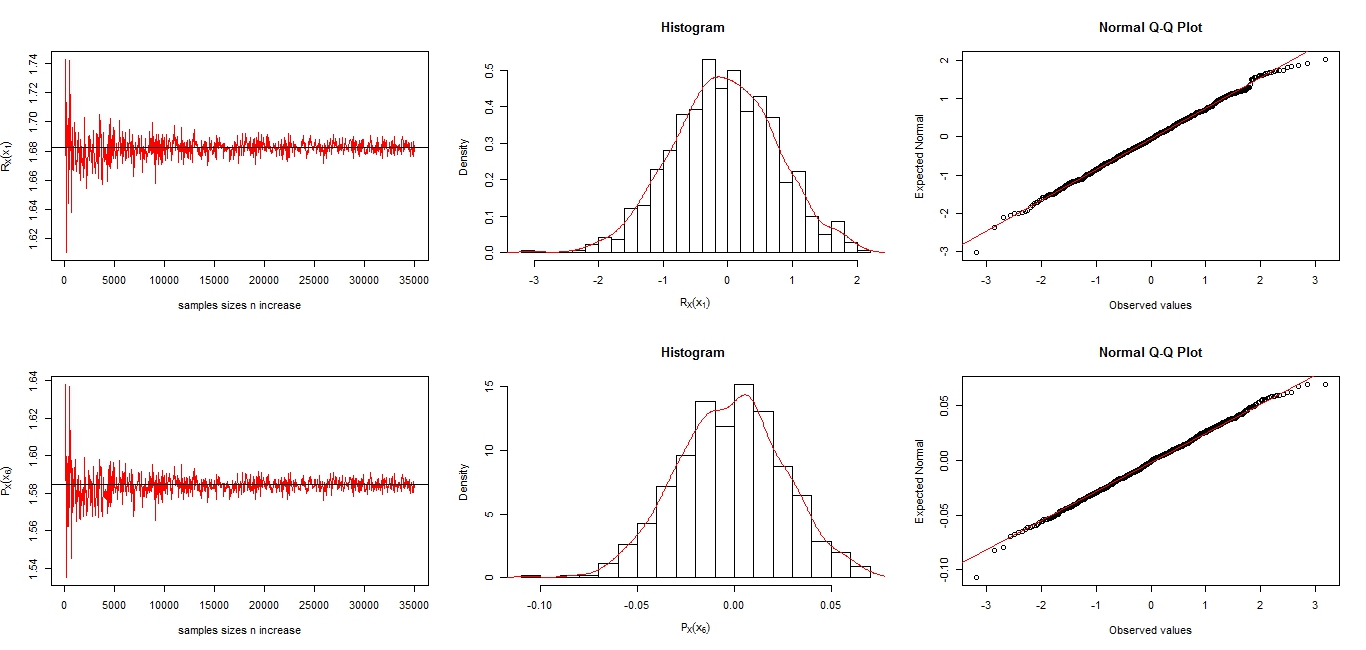
Figure 1. Plots of $\mathcal{R}_{X}^{(n)}(1)$ and $\mathcal{P}_{X}^{(n)}(6)$ when samples sizes increase, histograms and normal Q-Q plots versus $\mathcal{N}(0,1)$. The distribution of $X$ being that of the Weibull distribution of type $II$ with maximum lifetime $r=6$ and shape parameter $\beta=2$.

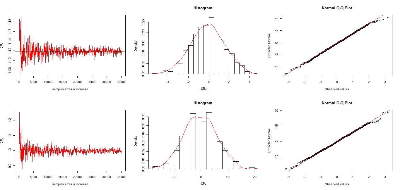
Figure 2. Plots of $\mathcal{CR}_{X}^{(n)}$ and $\mathcal{CP}_{X}^{(n)}$ when samples sizes increase, histograms and normal Q-Q plots versus $\mathcal{N}(0,1)$. The distribution of $X$ being that of the Weibull distribution of type $II$ with maximum lifetime $r=6$ and shape parameter $\beta=2$.

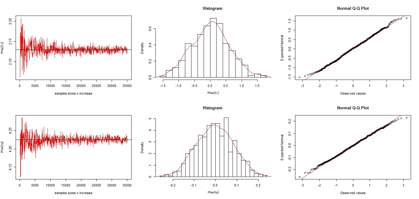
Figure 3. Plots of $\mu_{R}^{(n)}(1)$ and $\mu_{P}^{(n)}(6)$ when samples sizes increase, histograms and normal Q-Q plots versus $\mathcal{N}(0,1)$. The distribution of $X$ being that of the Weibull distribution of type $II$ with maximum lifetime $r=6$ and shape parameter $\beta=2$.

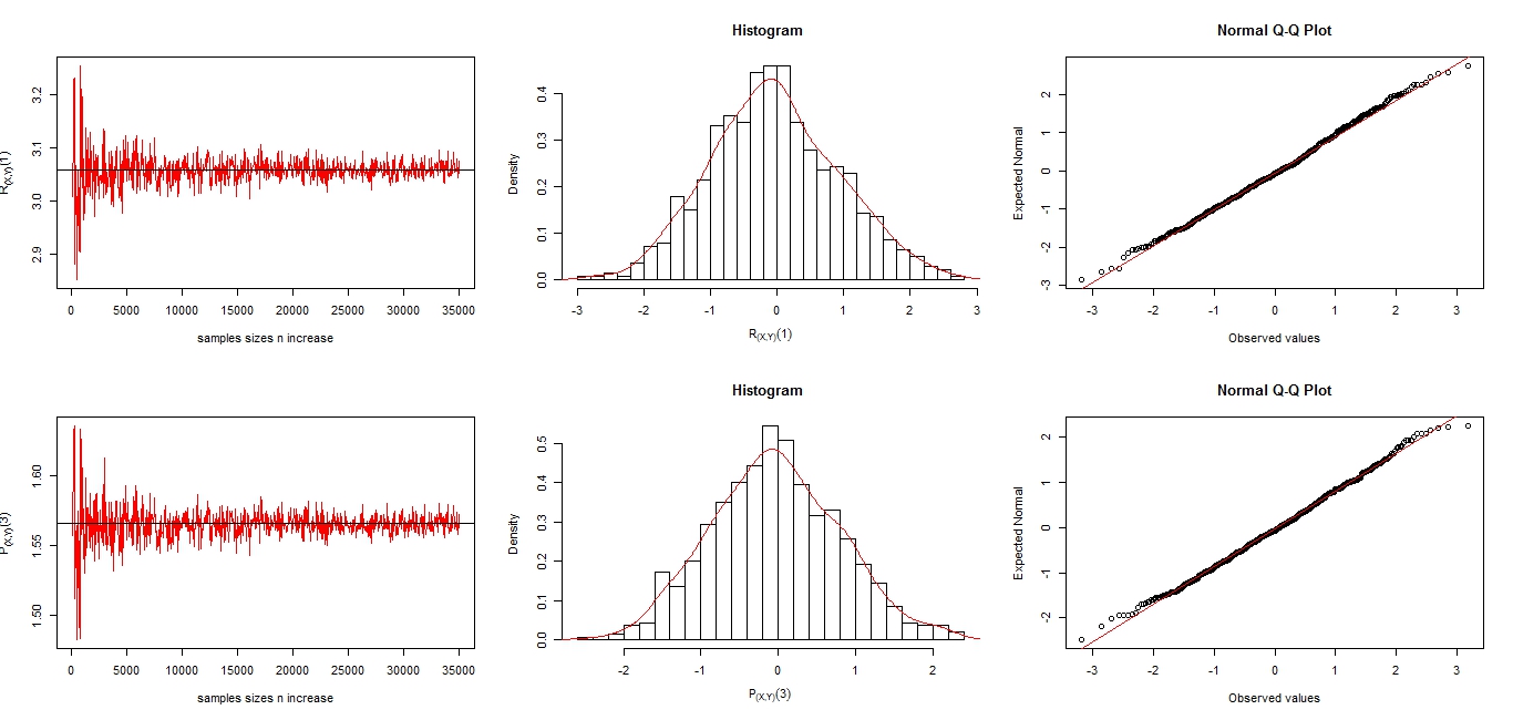
Figure 4. Plots of $\mathcal{R}_{(X,Y)}^{(n)}(1)$ and $\mathcal{P}_{(X,Y)}^{(n)}(3)$ when samples sizes increase, histograms and normal Q-Q plots versus $\mathcal{N}(0,1)$. $X$ and $Y$ being two random variables which p.m.f.’s are given respectively by (4.1) and (4.2).

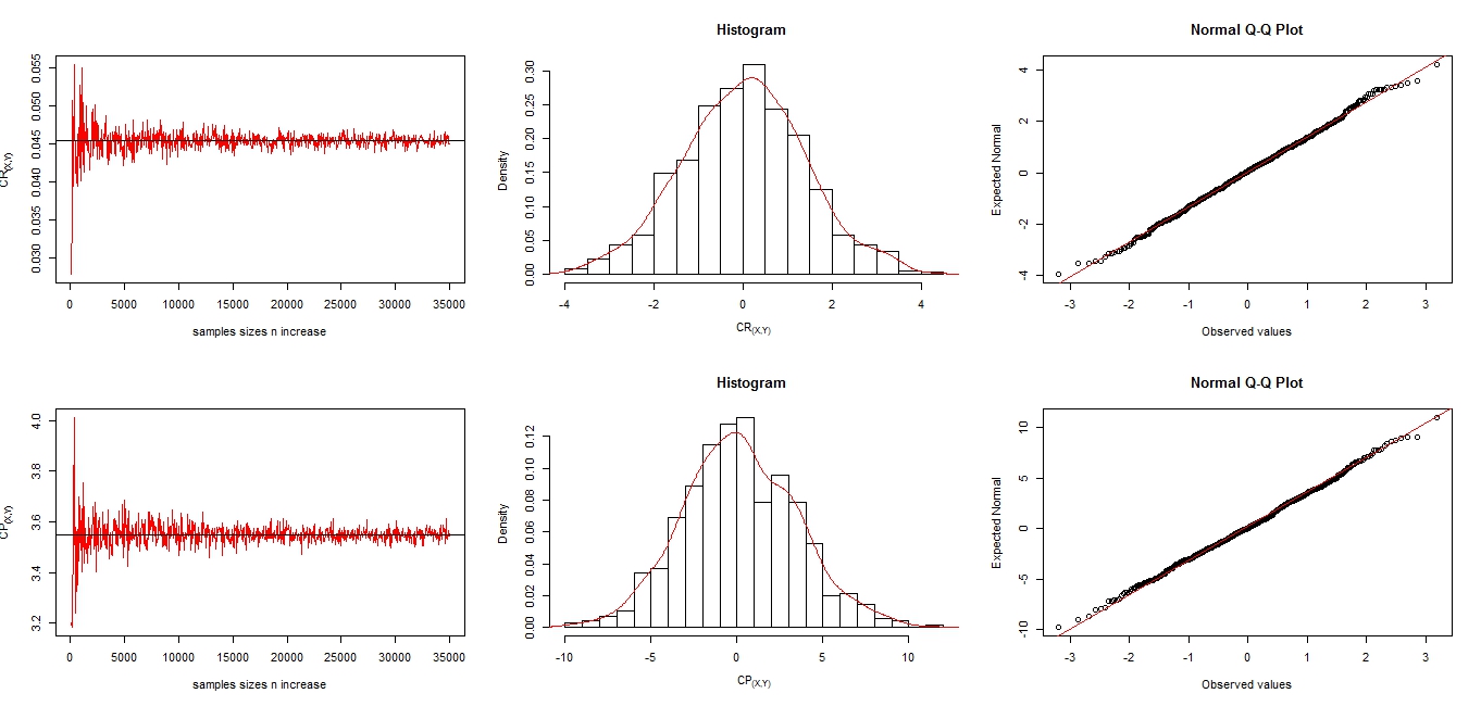
Figure 5. Plot of $\mathcal{CR}_{(X,Y)}^{(n)}$ and $\mathcal{CP}_{(X,Y)}^{(n)}$ when samples sizes increase, histograms and normal Q-Q plots versus $\mathcal{N}(0,1)$. $X$ and $Y$ being two random variables which p.m.f.’s are given respectively by (4.1) and (4.2).

References

• Shannon (1948) C. E. Shannon, A mathematical theory of communication, The Bell System Technical Journal, Vol.27, No.3, pp. 379-423.
• Ebrahimi and Pellerey (1995) Ebrahimi, N. and Pellerey, F. (1995). New partial ordering of survival functions based on notion of uncertainty, Journal of Applied Probability, 32, pp. 202-211.
• Belzunce et al. (2004) Belzunce, F., Navarror, J., Ruiz, J.M. and Aguila, Y., (2004), ”Some results on residual entropy function”. Metrika 59:147-161.
• Chandra and Roy (2001) Chandra, N.K. and Roy, D., (2001), ”Some results on reversed hazard rate”. Prob. Eng. Inf. Sci. 15: 95-102.
• Di Crescenzo and Longobardi (2004) Di Crescenzo, A. and Longobardi, M. (2004), A measure of discrimination between past lifetime distributions. Stat. Prob. Lett. 67, 173–182.
• Mervat (2013) Mervat Mahdy (2013). Probabilistic Properties of Discrete Mean and Variance Reversed Residual Lifetime Functions. Applied Mathematical Sciences, Vol.7, $N.$ 124, 6167-6179.
• Crescenzo and Longobardi (2009) A. Di Crescenzo, M. Longobardi(2009). On cumulative entropies, Journal of Statistical Planning and Inference 139 , no. 12, 4072–4087
• Ebrahimi (1996) Ebrahimi, N., (1996). How to measure uncertainty in the residual life time distribution. Sankhya Ser. A 58, 48–56.
• Di Crescenzo et al. (2004) Di Crescenzo, A., Longobardi M. and Nastro, A. (2004), On the mutual information between residual lifetime distributions. In: Cybernetics and Systems 2004, Vol. 1 (R. Trappl, Ed.), p. 142–145. Austrian Society for Cybernetic Studies, Vienna. ISBN 3-85206-169-5.
• Kerridge (1961) Kerridge, D. F. (1961). Inaccuracy and inference. Journal of the Royal Statistical Society: Series B, 23, 184-194.
• Hall (1987) Hall,P. (1987). On Kullback-Leibler loss and density estimation. The Annals of Statistics, Vol.15(4), pp.1491-1519.
• Singh and Poczos (2014) Singh S. and Poczos, B. (2014). Generalized Exponential Concentration Inequality for RΓ©nyi Divergence Estimation. Journal of Machine Learning Research.Vol.6. Carnegie Mellon University.
• Krishnamurthy et al. (2014) Akshay K., Kirthevasan K., Poczos B., and Wasserman, L.(2014). Nonparametric Estimation of RΓ©nyi Divergence and Friends. Journal of Machine Learning Research Workshop and conference Proceedings, 32. Vol.3, pp. 2.
• Ba et al. (2019) Ba, A.D, Lo G.S.(2019), Divergence Measures Estimation and Its Asymptotic Normality Theory in the discrete case. European Journal of Pure and Applied Mathematics, Vol.12, No.3, 790-820.
• Lo (2016) Lo, G.S.(2016). Weak Convergence (IA). Sequences of random vectors. SPAS Books Series. Saint-Louis, Senegal - Calgary, Canada. Doi : 10.16929/sbs/2016.0001. Arxiv : 1610.05415. ISBN : 978-2-9559183- 1-9.
• Valiron (1966) Georges Valiron. Cours d’analyse mathΓ©matique. Masson et Cie, 1966.
• Kayid and Ahmad (2004) M. Kayid, I.A. Ahmad, On the mean inactivity time ordering with reliability applications, Probab. Eng. Inform. Sci. 18 (2004) 395-409.
• Misra et al. (2008) N. Misra, N. Gupta, I.D. Dhariyal, Stochastic properties of residual life and inactivity time at a random time, Stoch. Models 24 (2008) 89–102.
• Nair and Gupta (2007) Nair, N.U. and Gupta, R. P. (2007). Characterization of proportional hazard models by properties of information measures. International Journal of Statistical Sciences, 6, 223-231.
• Taneja et al. (2009) Taneja, H. C., Kumar, V. and Srivastava, R. (2009). A dynamic measure of inaccuracy between two residual lifetime distributions. International Mathematical Forum, 4(25), 1213-1220.
• Thapliyal and Taneja (2013) Thapliyal, R., Taneja, H.C., 2013. A measure of inaccuracy in order statistics. J. Stat. Theory Appl. 12(2), 200-207.
• Kumar et al. (2011) Kumar, V., Taneja, H.C. and Srivastava, R. (2011). A dynamic measure of inaccuracy between two past lifetime distributions. Metrika, 74(1), 1-10.
• Osman (2017) Osman Kamari(2017). Characterizations Based on Cumulative Entropy of the Last-order Statistics . International Journal of Statistics and Probability; Vol. 6, No. 3; May 2017 Published by Canadian Center of Science and Education
• Rao et al. (2004) Murali Rao, Yunmei Chen, Baba C. Vemuri, Fellow, IEEE, and Fei Wang (2004). Cumulative Residual Entropy: A New Measure of Information IEEE TRANSACTIONS ON INFORMATION THEORY, VOL. 50, No. 6, JUNE 2004
• Khorashadizadeh et al. (2012) M. Khorashadizadeh, A.H. Rezaei Roknabadi and G.R. Mohtashami Borzadaran(2012), Characterizations of lifetime distributions based on doubly truncated mean residual life and mean past to failure, Communications in Statistics: Theory and Methods, 41, 6, 1105-1115.
• Rao et al. (2004) Rao, M., Chen, Y., Vemuri, B. C. and Wang, F. (2004). Cumulative residual entropy: a new measure of information. IEEE Transactions on Information Theory,50(6), 1220-1228.
• Rajesha et al (2015) G. Rajesha, E. I. Abdul-Satharb, R. Mayab and K. R. Muraleedharan Nairc (2015). Nonparametric estimation of the residual entropy function with censored dependent data . Journal of Probability and Statistics, Vol. 29, No.4, 866-877 DOI: 10.1214/14-BJPS250 .
• Drissi et al. (2008) Drissi, N., Chonavel, T., and Boucher, J. M. (2008). Generalized cumulative residual en- tropy for distributions with unrestricted supports. Research letters in signal processing, 11.
• Sunoj and Linu (2012) Sunoj, S. M. and Linu, M. N. (2012). Dynamic cumulative residual Renyi’s entropy. Statistics, 46(1), 41-56.
• Psarrakos and Navarro (2013) Psarrakos, G. and Navarro, J. (2013). Generalized cumulative residual entropy and record values. Metrika, 76(5), 623-640.
• Rajesh and Sunoj (2016) Rajesh, G. and Sunoj, S. M. (2016). Some properties of cumulative Tsallis entropy of order alpha. Statistical Papers, 1-11, doi:10.1007/s00362-016-0855-7.
• Bracquemond and Gaudoin (2003) Cyril Bracquemond and Olovier Gaudoin (2003). A survey on discrete lifetime distributions International Journal of Reliability, Quality and Safety Engineering/ Vol. 10, No. 01, pp. 69-98.
• Yang (1978) Grace L. Yang (1978). Estimation Of biomedical function, The Annals of Statistics, Vol.6, No.1, 112-116.
• Ba et al. (2016) Ba A.D, Lo G.S, Seck T. Deme El (2016). Consistency bands for mean excess function and application to graphical goodness of fit test for financial data. Journal of Mathematics Research, Vol. 8, No1.
• Hall,W.J. and Wellner (1981) Hall,W.J. and Wellner,J.A.(1981). Mean residual life.. In: Csorgo, M.,Dawson, D.A., Rao, J.N.K., Saleh, A.K.Md.E.( Eds), Statistics and Related Topics. North-Holland, Amsterdam, pp. 169-184.
• Enchakudiyil and Glory (2018) Enchakudiyil I. A. S. and Glory S. S.(2018). Estimation of dynamic cumulative past entropy for power function distribution. STATISTICA, anno LXXVIII, n. 4.
• Sepehrifar (2006) M.B. Sepehrifar (2006), Modeling and characterizations of new notions in life testing with statistical applications, University of Central Florida Orlando, Florida.
• Athanasios and Papaioannou (2012) Athanasios Sachlas and Takis Papaioannou (2012). Residual and Past Entropy in Actuarial Science and Survival Models Methodol Comput Appl Probab DOI 10.1007$/$s11009-012-9300-0
• Lai and Wang (1995) Lai C.D and Wang D.Q. (1995). A finite range discrete life distribution. International Journal of reliability, Quality and Safety Engineering Vol.2n No2, 147-160.
• Zohrevand et al. (2016) Zohrevand, Y., Hashemi, R. and Asadi, M. β€œA short note on the cumulative residual entropy”. The 2nd Workshop on Information Measures and their Applications, 54-57, 201528-29 January, 2015, Ferdowsi Univ. of Mashad, Iran.
• Kundu et al. (2016) Kundu, C., Di Crescenzo, A. and Longobardi, M. (2016), On cumulative residual (past) inaccuracy for truncated random variables. Metrika, 79(3), 335-356.
• Asadi and Zohrevand (2007) Asadi, M. and Zohrevand, Y. (2007). On the dynamic cumulative residual entropy. Journal of Statistical Planning and Inference, 137(6), 1931-1941
• Tahmasebi et al. (2018) Saeid Tahmasebi, Ahmad Nezakati, Safeih Daneshi (2018). Results on Cumulative Measure of Inaccuracy in Record Values Journal of Statistical Theory and Applications, Vol. 17, No.1 (March 2018) 15-28
• Di Crescenzo and Longobardi (2002) Di Crescenzo and Longobardi(2002)
• Nanda and Paul (2006) Nanda, A.K. and Paul, P. (2006b). Some properties of past entropy and their applications, Metrika, 64(1), pp. 47-61.
• Sati $\&$ Gupta (2015) M.M. Sati, N. Gupta (2015), Some characterization results on dynamic cumulative residual Tsallis entropy, J Probab. Stat.