plain(##3)  nonumberplain

Proximal Splitting Algorithms
for Convex Optimization:
A Tour of Recent Advances, with New Twists

Abstract

Convex nonsmooth optimization problems, whose solutions live in very high dimensional spaces, have become ubiquitous. To solve them, the class of first-order algorithms known as proximal splitting algorithms is particularly adequate: they consist of simple operations, handling the terms in the objective function separately. In this overview, we demystify a selection of recent proximal splitting algorithms: we present them within a unified framework, which consists in applying splitting methods for monotone inclusions in primal-dual product spaces, with well-chosen metrics. Along the way, we easily derive new variants of the algorithms and revisit existing convergence results, extending the parameter ranges in several cases. In particular, we emphasize that when the smooth term in the objective function is quadratic, e.g., for least-squares problems, convergence is guaranteed with larger values of the relaxation parameter than previously known. Such larger values are usually beneficial for the convergence speed in practice.

Key words.  large-scale convex optimization, nonsmooth optimization, splitting, proximal algorithm, primal-dual algorithm

MSC codes.. 90C25, 90C30, 90C06, 47J25, 47J26, 68W15, 65K05

1 Introduction

Optimization, also called mathematical programming, is the search for a best object in a set with respect to some criterion. Mathematically, this amounts to characterizing a point where a function attains its minimum value, and computationally, this often consists in exhibiting an iterative algorithm in which a variable converges to such an optimal point. When a function is convex, its minimizers are global: a point which attains a minimum value in its neighborhood is actually optimal in the whole search space. Thus, it is important to know about the principles behind convex optimization algorithms, before considering more general problems. This paper is a constructive and self-contained introduction to the class of proximal splitting algorithms, which are efficient for large-scale convex optimization.

Many problems in statistics, machine learning, signal and image processing, control, and many other fields can be formulated as convex optimization problems [99, 123, 4, 107, 29, 124] of the form:

$$\operatorname*{minimize}_{x\in\mathcal{X}}\,\sum_{m=1}^{M}g_{m}(L_{m}x),$$ (1.1)

for some $M\geq 1$, where $\mathcal{X}$ is a real Hilbert space, the $g_{m}$ are convex, possibly nonsmooth, functions, and the $L_{m}$ are linear operators. We will see that this generic formulation encompasses the possible presence of constraints. In the age of “big data,” with the explosion in size and complexity of the data to process, it is increasingly important to be able to solve such optimization problems, whose solutions live in very high dimensional spaces [63, 122, 19, 64, 106]. For instance, in image processing and computer vision, there are one or several variables to estimate for each pixel, with typically several millions of pixels. There is an extensive literature on proximal splitting algorithms for solving convex optimization problems, with applications in various fields [41, 122, 10, 100, 84, 117, 74, 52, 8, 44]. They consist of simple, easy-to-compute steps that can deal with the terms in the objective function separately: if a function is smooth, its gradient can be used, whereas for a nonsmooth function, the proximity operator will be called instead (hence the wording proximal algorithm). Since the proximity operator of a sum of functions does not have a computable form, in general, it is necessary to handle individually the proximity operators of the functions that appear in the problem; this is what splitting refers to, a notion reminiscent to the divide-and-conquer principle, which is ubiquitous in computational sciences.

It has been known for several decades that the dual problem, associated to the (primal) optimization problem under consideration, can be easier to solve and, if used, may simplify the computation of the primal solution. Yet, the development of primal-dual algorithms, which solve the primal and dual problems simultaneously, in an intertwined way, is more recent. In this tutorial survey, we introduce a selection of primal-dual proximal splitting algorithms, which have been developed over the last decade. We present them in a unified way, by solving a monotone inclusion expressed in a well-chosen primal-dual product space. Along the way, some new variants are naturally obtained. An important idea for the development of primal-dual algorithms is preconditioning, or equivalently changing the metric of the ambient Hilbert space [105, 45, 13]. We will make extensive use of this notion throughout the paper.

In our presentation, we put the emphasis on the potential to overrelax the algorithms: let us consider an algorithm producing a new estimate $z^{(i+\frac{1}{2})}$ of some variable at iteration number $i+1$, given the previous estimate $z^{(i)}$. Instead of setting $z^{(i+1)}=z^{(i+\frac{1}{2})}$ before continuing with the next iteration, overrelaxation consists in the extrapolated update $z^{(i+1)}=z^{(i)}+\rho^{(i)}(z^{(i+\frac{1}{2})}-z^{(i)})$, for some $\rho^{(i)}>1$. This step is easy to implement and can improve the convergence speed of the algorithm. Thus, it is important to study the conditions on the parameters $\rho^{(i)}$ that guarantee convergence. In particular, we show that if the optimization problem involves a smooth term that is quadratic, convergence is guaranteed with larger values of the relaxation parameter than previously known. Regularized least-squares problems are an important class of problems to which this extension applies.

Also, a desirable property of the proximal splitting algorithms is that they can be parallelized. Thus, when minimizing the sum of a large number of functions on a parallel computing architecture, each processor can handle one of the functions. Mathematical splitting gracefully blends into the physical splitting of the computing hardware in that case. The need for such parallel optimization algorithms is rapidly growing in distributed or federated learning [85, 82, 91] and artificial intelligence. The last part of the paper is dedicated to parallel versions of the algorithms.

The paper is organized as follows. In section 2, we present the most important notions and principles underlying the class of iterative algorithms for large-scale convex nonsmooth optimization under study. In section 3, we present relaxed versions of the forward-backward splitting algorithm to solve monotone inclusions. This analysis is subsequently applied in section 4 to the Loris–Verhoeven algorithm, which is a primal-dual forward-backward algorithm. In section 5, we analyze the Chambolle–Pock algorithm and its particular case, the Douglas–Rachford algorithm, which is equivalent to the Alternating Direction Method of Multipliers (ADMM). For these too, we derive convergence results for relaxed versions, which extend previously known results. In section 6, we study an algorithm that we call the Generalized Chambolle–Pock algorithm, since it is applicable to the minimization of two functions composed with two linear operators and reverts back to the Chambolle–Pock algorithm when one of the linear operators is the identity. The algorithm has been presented in the literature as a linearized or preconditioned version of the ADMM, but without relaxation. In section 7, we study an algorithm proposed independently by the first author and by B. C. Vũ that is also a primal-dual forward-backward algorithm. Section 8 is devoted to recently proposed algorithms based on a three-operator splitting scheme, which can be viewed as the fusion of the forward-backward and Douglas–Rachford two-operator splitting schemes. Along the way, new algorithm variants are proposed, for example, in subsections 7.1 and 8.1. Finally, in section 9, we propose parallel versions of all these algorithms by applying them in product spaces.

2 A Brief Introduction to Convex Analysis and Fixed-Point Algorithms

2.1 Notions of convex analysis

In this section, we introduce some notions and notations that will be used throughout the paper. The reader can find a much more complete account of convex analysis and operator theory in textbooks, e.g., [12, 7], or in papers like [117, 39].

We consider optimization over real Hilbert spaces: a real Hilbert space is a vector space equipped with a real inner product $\langle\cdot\,,\cdot\rangle$. When we make use of a norm without further specification, this is the norm $\|\cdot\|=\langle\cdot\,,\cdot\rangle^{1/2}$ induced by the inner product. This general formalism allows us to optimize with respect to vectors, matrices, or tensors [69], which are real-valued or complex-valued with some Hermitian properties, but also more complicated objects like quaternions [95]. The Hilbert spaces can be of infinite dimension; this can be useful in control [135] or when solving PDEs, and we will see that most results hold in this general setting. However, there are a few technicalities to keep in mind:

1) Let $L:\mathcal{X}\rightarrow\mathcal{U}$ be a linear operator, with $\mathcal{X}$ and $\mathcal{U}$ two real Hilbert spaces. We define the operator norm of $L$ as $\|L\|=\sup\{\|Lx\|:x\in\mathcal{X}$ and $\|x\|\leq 1\}$. If $\|L\|<+\infty$, $L$ is said to be bounded. $L$ is bounded if and only if it is continuous. In the paper, we will assume all linear operators to be bounded. If $\mathcal{X}$ is of finite dimension, $L$ is necessarily bounded.

2) A sequence of points $(x^{(i)})_{i\in\mathbb{N}}$ in a real Hilbert space $\mathcal{X}$ is said to converge weakly to a point $x^{\star}\in\mathcal{X}$ if, for every $y\in\mathcal{X}$, $\langle x^{(i)},y\rangle\rightarrow\langle x^{\star},y\rangle$. On the other hand, $(x^{(i)})_{i\in\mathbb{N}}$ is said to converge strongly to $x^{\star}\in\mathcal{X}$ if $\|x^{(i)}-x^{\star}\|\rightarrow 0$. Strong convergence implies weak convergence. If $\mathcal{X}$ is of finite dimension, both notions are equivalent and we just say that $(x^{(i)})_{i\in\mathbb{N}}$ converges to $x^{\star}$. We will see that most convergence results state weak convergence; this is not a weakness of the proof techniques, and strong convergence in infinite-dimensional spaces cannot be guaranteed without further assumptions [20]. In particular, given a continuous operator $T$ on $\mathcal{X}$, if a sequence $(x^{(i)})_{i\in\mathbb{N}}$ converges weakly to $x^{\star}\in\mathcal{X}$, one cannot deduce that $\big{(}T(x^{(i)})\big{)}_{i\in\mathbb{N}}$ converges weakly to $T(x^{\star})$. This makes the convergence proofs of algorithms more difficult to derive.

For the rest of section 2, let $\mathcal{X}$ be a real Hilbert space. A subset $\Omega$ of $\mathcal{X}$ is said to be convex if, for every $(x,y)\in\Omega^{2}$ and $a\in(0,1)$, $ax+(1-a)y\in\Omega$. Note that a convex set can be open, like the interval $(0,1)$ in $\mathbb{R}$, or closed, like $[0,1]$; it can be bounded or unbounded, like $[0,+\infty)$. The intersection of convex sets is convex. The union of convex sets is not convex, in general.

A function $f:\mathcal{X}\rightarrow\mathbb{R}\cup\{+\infty\}$ is said to be convex if, for every $(x,y)\in\mathcal{X}^{2}$ and $a\in(0,1)$,

$$f\big{(}ax+(1-a)y\big{)}\leq af(x)+(1-a)f(y).$$ (2.1)

We note that $f$ is allowed to take the value $+\infty$, a distinctive and very useful feature of convex analysis, compared to classical analysis. For calculus, we only need to adopt the following rules: for every $t>0$, $t(+\infty)=+\infty$, and for every $t\in\mathbb{R}$, $t+(+\infty)=+\infty$. Note that for every $t\in\mathbb{R}$, the intervals $(t,+\infty]$ are considered open in $\mathbb{R}\cup\{+\infty\}$, so that, for instance, the function $t\in\mathbb{R}\mapsto(1/t$ if $t>0$, $+\infty$ otherwise$)$ is continuous on $\mathbb{R}$ [7, Example 1.22]. The domain of $f$ is the convex set $\mathrm{dom}\,f=\{x\in\mathcal{X}:f(x)\neq+\infty\}$. $f$ is said to be proper if its domain is nonempty.

Indicator functions relate the two notions of convexity of a set and of a function: given a set $\Omega\subset\mathcal{X}$, we define the indicator function of $\Omega$, denoted by $\imath_{\Omega}$, as:

$$\imath_{\Omega}:x\in\mathcal{X}\mapsto\left\{\begin{array}[]{ll}0&\mbox{if }x\in\Omega,\\ +\infty&\mbox{otherwise}.\end{array}\right.$$ (2.2)

Then, if $\Omega$ is convex, $\imath_{\Omega}$ is convex; if $\Omega$ is nonempty, $\imath_{\Omega}$ is proper. Also, given two convex sets $\Omega_{1}\subset\mathcal{X}$ and $\Omega_{2}\subset\mathcal{X}$,

$$\imath_{\Omega_{1}\cap\Omega_{2}}=\imath_{\Omega_{1}}+\imath_{\Omega_{2}}.$$ (2.3)

Indicator functions are important, since they allow us to remove constraints and integrate them into the objective function to minimize. Indeed, given a nonempty convex set $\Omega\subset\mathcal{X}$ and a convex function $f$ on $\mathcal{X}$,

$$\operatorname*{minimize}_{x\in\Omega}\,f(x) \ \equiv\ \operatorname*{minimize}_{x\in\mathcal{X}}\,f(x)\ \ \mbox{s.t.}\ \ x\in\Omega,$$ (2.4)

$$\ \equiv\ \operatorname*{minimize}_{x\in\mathcal{X}}\,f(x)+\imath_{\Omega}(x).$$ (2.5)

We see here the interest in allowing the functions to take the value $+\infty$: it is used to exclude some parts of $\mathcal{X}$ from the set of possible solutions. Thus, we will consider the problem of minimizing a sum of convex functions, knowing that, thanks to indicator functions, this covers the possible presence of constraints.

A convex optimization problem consists in estimating a minimizer $x^{\star}\in\mathcal{X}$, supposed to exist, of a proper convex function $f:\mathcal{X}\rightarrow\mathbb{R}\cup\{+\infty\}$, that is, a point $x^{\star}$ at which $f$ attains its minimum value $\min_{x\in\mathcal{X}}f(x)$. The set of minimizers of $f$, which is convex, is denoted by $\operatorname*{arg\,min}_{x\in\mathcal{X}}f(x)$. Thus, $x^{\star}\in\operatorname*{arg\,min}_{x\in\mathcal{X}}f(x)$ if and only if, for every $x\in\mathcal{X}$, $f(x^{\star})\leq f(x)$. Note that the function $t\in\mathbb{R}\mapsto(1/t$ if $t>0$, $+\infty$ otherwise$)$ is proper, convex, and bounded from below, but does not have any minimizer.

An optimization algorithm to minimize a proper convex function $f:\mathcal{X}\rightarrow\mathbb{R}\cup\{+\infty\}$, which has a minimizer, constructs a sequence $(x^{(i)})_{i\in\mathbb{N}}$ of points such that $f(x^{(i)})$ decreases overall. Thus, for the process to be fruitful, if $(x^{(i)})_{i\in\mathbb{N}}$ converges to $x^{\star}$, we must have $\lim\inf_{i\in\mathbb{N}}f(x^{(i)})\geq f(x^{\star})$. Otherwise, even if $f(x^{(i)})$ converges to $\min f$, we cannot deduce that $x^{\star}$ is a minimizer of $f$. So, we will only consider functions having this lower semicontinuity property. Equivalently, a function $f$ is said to be lower semicontinuous if the convex set $\{x\in\mathcal{X}:f(x)\leq t\}$ is closed for every $t\in\mathbb{R}$. A continuous function is lower semicontinuous. A proper convex lower semicontinuous function is continuous on the interior of its domain [7, Corollary 8.39], so that lower semicontinuity concerns the boundary of the domain, where the function jumps from real values to $+\infty$.

We denote by $\Gamma_{0}(\mathcal{X})$ the set of convex, proper, lower semicontinuous functions from $\mathcal{X}$ to $\mathbb{R}\cup\{+\infty\}$. We will only consider such functions in optimization problems. If $\Omega\subset\mathcal{X}$ is nonempty and closed, $\imath_{\Omega}\in\Gamma_{0}(\mathcal{X})$. If $f\in\Gamma_{0}(\mathcal{X})$ and $L$ is a bounded linear operator with values in $\mathcal{X}$, $f\circ L$ is convex and lower semicontinuous [7, Proposition 9.5], where $\circ$ denotes the composition of functions; it is proper if and only if $\mathrm{dom}\,f\cap\mathrm{ran}\,L\neq\emptyset$, where $\mathrm{ran}\,L$ denotes the range of $L$. Also, if $f\in\Gamma_{0}(\mathcal{X})$ and $g\in\Gamma_{0}(\mathcal{X})$, $f+g$ is convex and lower semicontinuous [7, Corollary 9.4]; it is proper if and only if $\mathrm{dom}\,f\cap\mathrm{dom}\,g\neq\emptyset$.

The difficulty of convex optimization stems from the fact that even if $f$ and $g$ are two simple convex functions with known minimizers, $f+g$ is difficult to minimize, in general. A well-known example is the LASSO problem [128], which consists in minimizing over $x\in\mathcal{X}$ the function $\|Lx-b\|^{2}+\|x\|_{1}$, where $L$ is a linear operator, $b$ an element, and $\|\cdot\|_{1}$ is the $l_{1}$ norm; note that every norm on $\mathcal{X}$ is convex. The minimizer of the least-squares term can be obtained efficiently by solving a linear system, the minimizer of the $l_{1}$ norm is the zero element, but there is no straightforward way of finding a minimizer of the sum of the two terms, in general. Algorithms able to solve such problems are precisely the purpose of this paper.

When dealing with vectors, a linear operator can be represented by a matrix, so that the application of a linear operator to a vector can be viewed as a matrix-vector product. But since we are placing ourselves in the general setting of Hilbert spaces, some definitions are in order. Let $L:\mathcal{X}\rightarrow\mathcal{U}$ be a bounded linear operator for some real Hilbert space $\mathcal{U}$. The adjoint operator $L^{*}:\mathcal{U}\rightarrow\mathcal{X}$ of $L$ is the only bounded linear operator such that $\langle Lx,u\rangle_{\mathcal{U}}=\langle x,L^{*}u\rangle_{\mathcal{X}}$ for every $x\in\mathcal{X}$ and $u\in\mathcal{U}$, where we have denoted by $\langle\cdot,\cdot\rangle_{\mathcal{X}}$ and $\langle\cdot,\cdot\rangle_{\mathcal{U}}$ the inner products in $\mathcal{X}$ and $\mathcal{U}$, respectively, to differentiate them. $L$ is said to be self-adjoint if $L^{*}=L$. We have $\|L\|=\|L^{*}\|=\sqrt{\|LL^{*}\|}=\sqrt{\|L^{*}L\|}$. $\mathrm{Id}$ denotes the identity operator. Let $P$ be a self-adjoint bounded linear operator on $\mathcal{X}$. $P$ is said to be positive if $\langle x,Px\rangle\geq 0$ for every $x\in\mathcal{X}$, and strongly positive if $P-a\mathrm{Id}$ is positive for some real $a>0$. If $P$ is positive, for every $y\in\mathcal{X}$, the function $x\mapsto\langle Px+y,x\rangle$ belongs to $\Gamma_{0}(\mathcal{X})$; for instance, with $P=\mathrm{Id}$ and $y=0$, we obtain that $\|\cdot\|^{2}\in\Gamma_{0}(\mathcal{X})$.

In this paper, we consider first-order algorithms; that is, which exploit information about the gradient or subdifferential of the functions. Let us define these notions. A continuous real-valued function $f\in\Gamma_{0}(\mathcal{X})$ is smooth, or differentiable, if at every $x\in\mathcal{X}$, there exists an element of $\mathcal{X}$, called the gradient of $f$ at $x$ and denoted by $\nabla f(x)$, such that for every $e\in\mathcal{X}$,

$$f(x+e)-f(x)-\langle e,\nabla f(x)\rangle=o(\|e\|),\quad\mbox{as }\|e\|\rightarrow 0.$$ (2.6)

That is, the affine function $y\mapsto f(x)+\langle y-x,\nabla f(x)\rangle$ is a first-order approximation of $f$ around $x$. Note that, as a consequence of convexity, this affine function is a minorant of $f$: for every $y\in\mathcal{X}$,

$$f(y)\geq f(x)+\langle y-x,\nabla f(x)\rangle.$$ (2.7)

Thus, $\nabla f$, the gradient of $f$, is the operator on $\mathcal{X}$: $x\mapsto\nabla f(x)$. It is continuous on $\mathcal{X}$ [7, Corollary 17.43]. For smooth functions $f$ and $g$, we have $\nabla(f+g)=\nabla f+\nabla g$, and for a linear operator $L$, $\nabla(f\circ L)=L^{*}(\nabla f)L$, where $AB$ denotes the composition of the two operators $A$ and $B$. We note that the gradient of the quadratic convex function $x\mapsto\langle Px+y,x\rangle$, for some positive self-adjoint bounded linear operator $P$ on $\mathcal{X}$ and some $y\in\mathcal{X}$, is $x\mapsto 2Px+y$.

We want to deal with nonsmooth functions; for instance, the absolute value function $f:\mathbb{R}\rightarrow\mathbb{R}:t\mapsto|t|$, and by extension the $l_{1}$ norm, are convex but not differentiable at $0$. Moreover, we allow convex functions to take the value $+\infty$. Thus, we need a more general notion than the gradient, which captures first-order information. This is where the subdifferential comes to the rescue. Let $f\in\Gamma_{0}(\mathcal{X})$. For every $x\in\mathcal{X}$, we define the subdifferential of $f$ at $x$, denoted by $\partial f(x)$, as the closed convex set [7, Proposition 16.4]

$$\partial f(x)=\big{\{}u\in\mathcal{X}\ :\ \forall y\in\mathcal{X},\ f(x)+\langle y-x,u\rangle\leq f(y)\big{\}}.$$ (2.8)

The elements of $\partial f(x)$ are called subgradients of $f$ at $x$. A subgradient $u\in\partial f(x)$ can be viewed as the gradient of the affine minorant $y\mapsto f(x)+\langle y-x,u\rangle$ of $f$. If $f$ is differentiable at $x$, there is only one subgradient, which is the gradient: $\partial f(x)=\{\nabla f(x)\}$. On the other hand, if $f(x)=+\infty$, $\partial f(x)=\emptyset$. A classical example is the function absolute value, for which $\partial|\cdot|(0)=[-1,1]$. Another example is $f:t\in\mathbb{R}\mapsto(0$ if $t\leq 0$, $+\infty$ otherwise$)$, for which $\partial f(0)=[0,+\infty)$. It is important to note that for any $g\in\Gamma_{0}(\mathcal{X})$ and $x\in\mathcal{X}$ [7, Proposition 16.6],

$$\partial f(x)+\partial g(x)\subset\partial(f+g)(x),$$ (2.9)

where the sum of the two sets is the Minkowski sum, but the inclusion may be strict [7, Remark 16.8]. Similarly, given a bounded linear operator $L$, for every $x\in\mathcal{X}$, $L^{*}\partial f(Lx)\subset\partial(f\circ L)(x)$. We denote by $2^{\Omega}$ the set of all subsets of a set $\Omega$. Then the subdifferential of $f$ is the set-valued operator $\partial f:\mathcal{X}\rightarrow 2^{\mathcal{X}},x\mapsto\partial f(x)$. We assimilate a set-valued operator $M:\mathcal{X}\rightarrow 2^{\mathcal{X}}$ with exactly one element in each set $M(x)$ as a single-valued operator $M:\mathcal{X}\rightarrow\mathcal{X}$, and conversely. For instance, for a smooth convex function $f$, we have $\partial f=\nabla f$.

We will consider convex optimization problems of the form:

$$\operatorname*{minimize}_{x\in\mathcal{X}}\,\sum_{m=1}^{M}g_{m}(L_{m}x),$$ (2.10)

where $M\geq 1$, each $L_{m}$ is a bounded linear operator from $\mathcal{X}$ to some real Hilbert space $\mathcal{U}_{m}$, possibly the identity if $\mathcal{U}_{m}=\mathcal{X}$, and each $g_{m}\in\Gamma_{0}(\mathcal{U}_{m})$. The well-known Fermat’s rule states that $x^{\star}\in\mathcal{X}$ is a solution to (2.10) if and only if

$$0\in\partial\Big{(}\sum_{m=1}^{M}g_{m}\circ L_{m}\Big{)}(x^{\star}).$$ (2.11)

This fundamental property is easy to demonstrate: let $f\in\Gamma_{0}(\mathcal{X})$ and $x^{\star}\in\mathcal{X}$. Then

$$x^{\star}\in\operatorname*{arg\,min}_{x\in\mathcal{X}}f(x) \Leftrightarrow\forall x\in\mathcal{X},\ f(x^{\star})\leq f(x)$$ (2.12)

$$\Leftrightarrow\forall x\in\mathcal{X},\ f(x^{\star})+\langle x-x^{\star},0\rangle\leq f(x)$$ (2.13)

$$\Leftrightarrow 0\in\partial f(x^{\star}).$$ (2.14)

As already mentioned in (2.9), for every $x\in\mathcal{X}$ we have

$$\Big{(}\sum_{m=1}^{M}L_{m}^{*}(\partial g_{m})L_{m}\Big{)}(x)\subset\partial\Big{(}\sum_{m=1}^{M}g_{m}\circ L_{m}\Big{)}(x),$$ (2.15)

but the inclusion may be strict. All algorithms considered in this paper actually find a solution $x^{\star}\in\mathcal{X}$ satisfying

$$0\in\sum_{m=1}^{M}L_{m}^{*}\partial g_{m}(L_{m}x^{\star}),$$ (2.16)

if such a solution exists. But in view of (2.15), the existence of a minimizer of $\sum_{m}g_{m}\circ L_{m}$ is not sufficient to guarantee the existence of a solution to (2.16). Therefore, throughout the paper, we assume that for every optimization problem considered, the solution set of the corresponding monotone inclusion (2.16) is nonempty. Given (2.15) and Fermat’s rule, a solution $x^{\star}$ of (2.16) is a solution to the optimization problem (2.10). If the functions satisfy a so-called qualification constraint, we have an equality instead of an inclusion in (2.15); in that case, it is sufficient to show that a solution to (2.10) exists. A qualification constraint is [42, Proposition 4.3]:

$$\bigcap_{m=1}^{M}L_{m}^{-1}(\mathrm{sri}\;\mathrm{dom}\;g_{m})\neq\emptyset,$$ (2.17)

where, for any linear operator $L:\mathcal{X}\rightarrow\mathcal{U}$ and $\Omega\subset\mathcal{U}$, $L^{-1}(\Omega)=\{x\in\mathcal{X}:Lx\in\Omega\}$, and $\mathrm{sri}\;\Omega$ denotes the strong relative interior of a convex set $\Omega$, which is the set of points $u\in\Omega$ such that the cone generated by $-u+\Omega$ is a closed linear subspace. Other qualification constraints can be found in [42, Proposition 4.3]. Note that for $\sum_{m=1}^{M}g_{m}\circ L_{m}$ to be proper, it is necessary to have $\cap_{m=1}^{M}L_{m}^{-1}(\mathrm{dom}\;g_{m})\neq\emptyset$. Since the strong relative interior is even larger than the interior of a set, the condition (2.17) is really not a lot to ask.

We have seen that the subdifferential is an important notion, in particular with Fermat’s rule. But the algorithms considered in this paper to solve optimization problems involving nonsmooth functions will not make use of subgradients directly. Instead, they will make calls to the proximity operators of the functions: we define the proximity operator [96] of any function $f\in\Gamma_{0}(\mathcal{X})$ as

$$\mathrm{prox}_{f}:\mathcal{X}\rightarrow\mathcal{X},x\mapsto\operatorname*{arg\,min}_{x^{\prime}\in\mathcal{X}}\Big{(}f(x^{\prime})+{\textstyle\frac{1}{2}}\|x^{\prime}-x\|^{2}\Big{)}.$$ (2.18)

By strong convexity of $f+\frac{1}{2}\|\cdot-x\|^{2}$, its minimizer always exists and is unique, so that the proximity operator is well defined. For any nonempty closed convex set $\Omega\subset\mathcal{X}$ and $\tau>0$,

$$\mathrm{prox}_{\tau\imath_{\Omega}}=\mathrm{proj}_{\Omega}:x\mapsto\operatorname*{arg\,min}_{x^{\prime}\in\Omega}\|x^{\prime}-x\|$$ (2.19)

is the projection onto $\Omega$, which does not depend on $\tau$. Thus, proximal algorithms can be viewed as generalizing algorithms to find points in intersections of convex sets [37]. Although the definition of the proximity operator is implicit, it has a closed form for many functions of practical interest. For instance, for the absolute value (and by extension for the $l_{1}$ norm by elementwise application), this is soft-thresholding: we have, for any $\tau>0$,

$$\mathrm{prox}_{\tau|\cdot|}:t\in\mathbb{R}\mapsto\mathrm{sign}(t)\max(|t|-\tau,0).$$ (2.20)

There are fast and exact methods to compute the proximity operators for a large class of functions [31, 41, 47, 49, 108, 62]; see also the website http://proximity-operator.net. In this paper, we consider proximal splitting algorithms, which are iterative algorithms producing an estimate of a solution to a convex optimization problem of the form (2.10), by calling at each iteration the proximity operator or the gradient of each function $g_{m}$, as well as the operators $L_{m}$ and $L_{m}^{*}$.

An optimization problem can often be written in the form (2.10) in several equivalent but different ways, with each formulation having appropriate algorithms to solve it. For instance, when a function $\imath_{\Omega}$ for some convex set $\Omega$ appears in the problem, it is implicitly assumed, in general, that one knows how to project onto $\Omega$. For instance, to minimize $f\in\Gamma_{0}(\mathcal{X})$ subject to the constraint $L\,\cdot=b$ for some linear operator $L$ and element $b$, the two following formulations are equivalent:

$$\operatorname*{minimize}_{x\in\mathcal{X}} \,f(x)+\imath_{\{x^{\prime}\in\mathcal{X}\ :\ Lx^{\prime}=b\}}(x),$$ (2.21)

$$\operatorname*{minimize}_{x\in\mathcal{X}} \,f(x)+\imath_{\{b\}}(Lx).$$ (2.22)

The first formulation is appropriate if one knows how to project on the affine constraint set efficiently, whereas the second formulation is preferable if one does not and asks for an algorithm making calls to $L$ and $L^{*}$.

For every $f\in\Gamma_{0}(\mathcal{X})$, we denote by $f^{*}$ the conjugate of $f$ defined by

$$f^{*}:x\mapsto\sup_{x^{\prime}\in\mathcal{X}}\big{(}\langle x,x^{\prime}\rangle-f(x^{\prime})\big{)},$$ (2.23)

which belongs to $\Gamma_{0}(\mathcal{X})$ as well. We have $f^{**}=f$. An important property is the Moreau identity, which allows us to compute the proximity operator of $f^{*}$ from that of $f$, and vice versa: for every $\tau>0$,

$$\mathrm{prox}_{\tau f}(x)=x-\tau\,\mathrm{prox}_{f^{*}/\tau}(x/\tau).$$ (2.24)

We do not define here further notions related to duality, which will be introduced progressively during the presentation of primal-dual algorithms.

2.2 Notions of operator theory and fixed-point algorithms

Let $M:\mathcal{X}\rightarrow 2^{\mathcal{X}}$ be a set-valued operator; as mentioned above, single-valued operators can be viewed as set-valued operators, so that the subsequent notions apply to them as well. The graph of $M$ is the set $\{(x,v)\in\mathcal{X}^{2}:v\in Mx\}$ (we may use the shortened notation $Mx$ for $M(x)$, usually adopted for linear operators, with any operator). The inverse operator of $M$, denoted by $M^{-1}$, is the set-valued operator with graph $\{(v,x)\in\mathcal{X}^{2}:v\in Mx\}$. That is, $v\in Mx$ if and only if $x\in M^{-1}v$. For instance, for any bounded linear operator $L$, $L^{-1}$ is well defined everywhere, in this sense. But $L^{-1}x$ can be the empty set if $x\notin\mathrm{ran}\,L$, or can contain several elements: $L^{-1}0$ is the kernel of $L$. The inverse relates the subdifferentials of a function $f\in\Gamma_{0}(\mathcal{X})$ and its conjugate $f^{*}\in\Gamma_{0}(\mathcal{X})$ defined in (2.23) via the simple relation [7, Corollary 16.30]:

$$\partial f^{*}=(\partial f)^{-1}.$$ (2.25)

$M$ is said to be monotone if, for every $(x,x^{\prime})\in\mathcal{X}^{2}$, $v\in Mx$, $v^{\prime}\in Mx^{\prime}$,

$$\langle x-x^{\prime},v-v^{\prime}\rangle\geq 0.$$ (2.26)

We note that for a self-adjoint bounded linear operator, being positive is equivalent to being monotone. A monotone operator $M$ is said to be maximally monotone if there exists no monotone operator whose graph strictly contains the graph of $M$. For every $f\in\Gamma_{0}(\mathcal{X})$,

$$\partial f\mbox{ is maximally monotone}$$ (2.27)

[7, Theorem 20.25]. The first derivative of a smooth convex function $f:\mathbb{R}\rightarrow\mathbb{R}$ is nondecreasing, so monotonicity can be viewed as a generalization of the nondecreasing property to multidimensional and set-valued operators. The problem of finding $x^{\star}$ such that $0\in Mx^{\star}$ is called a monotone inclusion. Thus, as we have seen with Fermat’s rule (2.10)–(2.11), convex optimization problems consist in solving monotone inclusions. This is why monotone operator theory plays an essential role in optimization.

If $M$ is monotone, we define its resolvent, denoted by $J_{M}$, as the operator

$$J_{M}=(M+\mathrm{Id})^{-1}.$$ (2.28)

$J_{M}$ is a well-defined single-valued operator on $\mathcal{X}$. Now, let us apply Fermat’s rule to the definition of the proximity operator in (2.18): if $y=\mathrm{prox}_{f}(x)$ for any $f\in\Gamma_{0}(\mathcal{X})$ and $x\in\mathcal{X}$, then $0\in\partial f(y)+y-x$. Equivalently, $y=(\partial f+\mathrm{Id})^{-1}(x)$. That is,

$$\mathrm{prox}_{f}=J_{\partial f}.$$ (2.29)

Thus, proximal algorithms handle nonsmooth functions by calls to their proximity operators; this can be viewed as a regularized and implicit way of dealing with their set-valued subdifferentials. But this comes at a price: $\mathrm{prox}_{f+g}$ cannot be expressed from $\mathrm{prox}_{f}$ and $\mathrm{prox}_{g}$, in general; in rare cases, $\mathrm{prox}_{f+g}=\mathrm{prox}_{f}\circ\mathrm{prox}_{g}$ [108]. Also $\mathrm{prox}_{f\circ L}$ does not have a computable form, in general. For instance, the proximity operator of the least-squares term $\frac{\tau}{2}\|L\cdot-b\|^{2}$ for some bounded linear operator $L:\mathcal{X}\rightarrow\mathcal{U}$, $b\in\mathcal{U}$ and $\tau>0$, is

$$x\mapsto(\tau L^{*}L+\mathrm{Id})^{-1}(x+\tau L^{*}b),$$ (2.30)

which has a closed form, but this amounts in practice to solving a linear system, which is generally too costly. Thus, even the apparently simple problem of minimizing the sum of two nonsmooth functions is in fact difficult. Thus, splitting is necessary: we have to call the proximity operator of each simple-enough function individually when minimizing a sum of functions, and deal with the linear operators separately.

Let $T:\mathcal{X}\rightarrow\mathcal{X}$ be a single-valued operator. A fixed point of $T$ is any $x^{\star}\in\mathcal{X}$ satisfying

$$x^{\star}=Tx^{\star}.$$ (2.31)

$T$ is said to be $\beta$-Lipschitz continuous for some real $\beta\geq 0$ if, for every $(x,x^{\prime})\in\mathcal{X}^{2}$,

$$\|Tx-Tx^{\prime}\|\leq\beta\|x-x^{\prime}\|.$$ (2.32)

We note that a bounded linear operator $L$ is $\|L\|$-Lipschitz continuous. $T$ is said to be nonexpansive if it is 1-Lipschitz continuous. $T$ is said to be $\alpha$-averaged for some $\alpha\in(0,1)$ if there exists a nonexpansive operator $T^{\prime}:\mathcal{X}\rightarrow\mathcal{X}$ such that

$$T=(1-\alpha)\mathrm{Id}+\alpha T^{\prime}.$$ (2.33)

If $T$ is $\alpha$-averaged for some $\alpha\in(0,1)$, it is $\alpha^{\prime}$-averaged for every $\alpha^{\prime}\in(\alpha,1)$ and nonexpansive; in addition, for every $\rho\in(0,\frac{1}{\alpha})$, the relaxed operator

$$\mathrm{Id}+\rho(T-\mathrm{Id})$$ (2.34)

is $\rho\alpha$-averaged. Firmly nonexpansive means $(1/2)$-averaged. Finally, $T$ is said to be $\xi$-cocoercive for some $\xi>0$ if $\xi T$ is firmly nonexpansive or, equivalently [7, Proposition 4.4], if, for every $(x,x^{\prime})\in\mathcal{X}^{2}$,

$$\xi\|Tx-Tx^{\prime}\|^{2}\leq\langle x-x^{\prime},Tx-Tx^{\prime}\rangle.$$ (2.35)

Let $\mathcal{Z}$ be a real Hilbert space and $T$ be a nonexpansive operator on $\mathcal{Z}$ with nonempty set of fixed points. A fixed-point algorithm, initialized with some $z^{(0)}\in\mathcal{Z}$, consists in iterating

$$z^{(i+1)}=Tz^{(i)},$$ (2.36)

where $i$ is the iteration counter and $z^{(i)}$ denotes the version of the variable $z$ produced during the $i$th iteration. Note that we have changed the name of the variable from $x$ to $z$ to emphasize that $z^{(i)}$ may not be the variable converging to a solution of the optimization problem at hand: it can be a concatenation of variables, like $z^{(i)}=(x^{(i)},u^{(i)})$, with $x^{(i)}$ converging to a desired solution and $u^{(i)}$ an auxiliary variable, the value of which is not of primary concern. Alternatively, it might be that there is an internal variable $x^{(i)}$ among the set of operations modeled by the abstract operator $T$, which converges to a solution, whereas $z^{(i)}$ is not interesting in itself.

Then, by combining (2.31) and (2.32), we have, for every fixed point $z^{\star}$ of $T$ and $i\geq 0$,

$$\|z^{(i+1)}-z^{\star}\|\leq\|z^{(i)}-z^{\star}\|.$$ (2.37)

Thus, the variable $z^{(i)}$ grows closer and closer at every iteration to the set of fixed points of $T$. But this is not sufficient to obtain convergence of the sequence $(z^{(i)})_{i\in\mathbb{N}}$ to some fixed point. A counterexample is the rotation operator of angle $\theta\in[0,2\pi)$ in $\mathbb{R}^{2}$, represented by the matrix

$$T=\left[\begin{array}[]{cc}\cos(\theta)&-\sin(\theta)\\ \sin(\theta)&\cos(\theta)\end{array}\right].$$ (2.38)

In that case the inequality in (2.37) is an equality, so that $(z^{(i)})_{i\in\mathbb{N}}$ generated by (2.36) turns over and over again in the plane and does not converge to the fixed point $(0,0)$ of $T$.

Thus, we have to be slightly more strict in our assumptions: we will suppose that $T$ in (2.36) is $\alpha$-averaged for some $\alpha\in(0,1)$, and not only nonexpansive. And in view of (2.34), given some sequence $(\rho^{(i)})_{i\in\mathbb{N}}$ of relaxation parameters, we will consider the relaxed iteration

$$\left\lfloor\begin{array}[]{l}z^{(i+\frac{1}{2})}=Tz^{(i)}\\ z^{(i+1)}=z^{(i)}+\rho^{(i)}(z^{(i+\frac{1}{2})}-z^{(i)}).\end{array}\right.$$ (2.41)

Note that with $\rho^{(i)}=1$, there is no relaxation and we recover the iteration (2.36). While there is no interest in doing underrelaxation with $\rho^{(i)}$ less than 1, overrelaxation with $\rho^{(i)}$ larger than 1 may be beneficial to the convergence speed, as is observed in practice in many cases. The idea of using overrelaxation comes from the following intuition: if the sequence $(z^{(i)})_{i\in\mathbb{N}}$ generated by (2.36) converges to some fixed point $z^{\star}$, this means that $z^{(i+1)}=Tz^{(i)}$ tends to be closer to $z^{\star}$ than $z^{(i)}$, on average. Hence, we may want, starting at $z^{(i)}$, to move further in the direction $Tz^{(i)}-z^{(i)}$, which improves the estimate. This is exactly what the relaxed iteration (2.41) does if $\rho^{(i)}>1$.

Now, we can state the fundamental result on which we will rely to establish convergence of optimization algorithms:

Krasnosel’skiĭ–Mann theorem (algorithm (2.41)) [7, Proposition 5.16]. Let $\mathcal{Z}$ be a real Hilbert space and let $T:\mathcal{Z}\rightarrow\mathcal{Z}$ be an $\alpha$-averaged operator for some $\alpha\in(0,1)$, with a nonempty set of fixed points. Let $(\rho^{(i)})_{i\in\mathbb{N}}$ be a sequence in $[0,1/\alpha]$, such that $\sum_{i\in\mathbb{N}}\rho^{(i)}(1-\alpha\rho^{(i)})=+\infty$. Let $z^{(0)}\in\mathcal{Z}$. Then the sequence $(z^{(i)})_{i\in\mathbb{N}}$ defined by the iteration (2.41) converges weakly to some fixed point $z^{\star}$ of $T$, and $(z^{(i+\frac{1}{2})}-z^{(i)})_{i\in\mathbb{N}}$ converges strongly to 0.

We note that as a direct implication of this theorem, $(z^{(i+\frac{1}{2})})_{i\in\mathbb{N}}$ converges weakly to the same fixed point $z^{\star}$. In practice, one might prefer to consider $z^{(i+\frac{1}{2})}$ instead of $z^{(i+1)}$ as an estimate of the solution, because it is in the range of $T$.

In this theorem, the assumption that $T$ has a nonempty set of fixed points is important: consider, for instance, $T=\mathrm{Id}+c$ for some $c\neq 0$, which is $\alpha$-averaged for every $\alpha\in(0,1)$. Then $T$ has no fixed point and the iteration (2.41) diverges.

Finally, we note that $\rho^{(i)}=1$ is allowed in the theorem. In practice, we recommend setting $\rho^{(i)}=1$ when running an algorithm for the first time, before trying larger values.

All algorithms presented in this paper are instances of the simple form (2.41), and their convergence analysis relies on the Krasnosel’skiĭ–Mann theorem.

It remains to see how to construct averaged operators whose fixed points are solutions to optimization problems. To that aim, we will combine gradients and proximity operators of functions like Lego bricks. Indeed, the set of averaged operators is stable by convex combinations (a convex combination is a linear combination with nonnegative weights whose sum is one) and compositions:

[7, Proposition 4.42] (convex combination of averaged operators). Let $(T_{m})_{m=1}^{M}$ be a family of operators for some $M\geq 1$, such that every $T_{m}:\mathcal{X}\rightarrow\mathcal{X}$ is $\alpha_{m}$-averaged for some $\alpha_{m}\in(0,1)$. Let $(\omega_{m})_{m=1}^{M}$ be real numbers in $(0,1]$, such that $\sum_{m=1}^{M}\omega_{m}=1$. Set $\alpha=\sum_{m=1}^{M}\omega_{m}\alpha_{m}\in(0,1)$ and $T=\sum_{m=1}^{M}\omega_{m}T_{m}$. Then $T$ is $\alpha$-averaged.

[98][7, Proposition 4.44] (composition of averaged operators). Let $T_{1}:\mathcal{X}\rightarrow\mathcal{X}$ be an $\alpha_{1}$-averaged operator and $T_{2}:\mathcal{X}\rightarrow\mathcal{X}$ be an $\alpha_{2}$-averaged operator for some $\alpha_{1}\in(0,1)$ and $\alpha_{2}\in(0,1)$. Set

$$\alpha=\frac{\alpha_{1}+\alpha_{2}-2\alpha_{1}\alpha_{2}}{1-\alpha_{1}\alpha_{2}}$$ (2.42)

and $T=T_{2}T_{1}$. Then $\alpha\in(0,1)$ and $T$ is $\alpha$-averaged.

Moreover, if $M:\mathcal{X}\rightarrow 2^{\mathcal{X}}$ is a maximally monotone operator,

$$J_{M}\mbox{ is firmly nonexpansive}$$ (2.43)

[7, Proposition 23.8]. And since the proximity operator is the resolvent of the subdifferential, it is firmly nonexpansive as well. Finally, when we deal with a smooth function using calls to its gradient, we will assume that the gradient is Lipschitz continuous. Indeed, the Baillon–Haddad theorem [7, Corollary 18.17] states the following: let $f:\mathcal{X}\rightarrow\mathbb{R}$ be a differentiable convex function whose gradient $\nabla f$ is $\beta$-Lipschitz continuous for some $\beta>0$. Then

$$\nabla f\mbox{ is }\textstyle\frac{1}{\beta}\mbox{-cocoercive}.$$ (2.44)

We now have all the ingredients to start designing algorithms. Let us start with the minimization of a differentiable convex function $f:\mathcal{X}\rightarrow\mathbb{R}$, whose gradient $\nabla f$ is $\beta$-Lipschitz continuous for some $\beta>0$, and whose set of minimizers is nonempty. Gradient descent, initialized at some $x^{(0)}\in\mathcal{X}$, consists in iterating, for $i\geq 0$,

$$x^{(i+1)}=x^{(i)}-\gamma\nabla f(x^{(i)})$$ (2.45)

for some parameter $\gamma\in(0,\frac{2}{\beta})$. It is called a descent method because one can show that $f(x^{(i+1)})\leq f(x^{(i)})$, so that the algorithm “goes down” along the function values. To analyze this algorithm, we first observe that $x^{(i+1)}=Tx^{(i)}$ for the operator $T=\mathrm{Id}-\gamma\nabla f$. Since $\frac{1}{\beta}\nabla f$ is firmly nonexpansive, it is easy to show that $T$ is $\alpha$-averaged with $\alpha=\frac{\gamma\beta}{2}\in(0,1)$. Moreover, $x^{\star}\in\mathcal{X}$ is a fixed point of $T$ if and only if $\nabla f(x^{\star})=0$, which is equivalent to $x^{\star}$ being a minimizer of $f$. Hence, we can invoke the Krasnosel’skiĭ–Mann theorem (without relaxation) to obtain weak convergence of the sequence $(x^{(i)})_{i\in\mathbb{N}}$ to a minimizer $x^{\star}$ of $f$.

We note that the relaxed version (2.41) with a fixed parameter $\rho$ of gradient descent simplifies to $x^{(i+1)}=x^{(i)}-\rho\gamma\nabla f(x^{(i)})$ with $\rho\gamma\in(0,\frac{2}{\beta})$, so that we can just set $\rho=1$ and keep $\gamma$ as the only parameter. How to choose the value of $\gamma$, then? As $\gamma$ tends to $\frac{2}{\beta}$, the operator $\mathrm{Id}-\gamma\nabla f$ is $\alpha$-averaged with $\alpha$ tending to 1, and we have seen that convergence is not guaranteed with merely nonexpansive operators. So, we can expect convergence to become slower as $\gamma$ tends to $\frac{2}{\beta}$; but this is true in the worst case: if $f=\frac{1}{2}\|\cdot\|^{2}$, whose gradient $\nabla f=\mathrm{Id}$ is $\beta=1$-Lipschitz continuous, we have $x^{(i+1)}=(1-\gamma)x^{(i)}$, and $\gamma=\frac{1}{\beta}=1$ is the best choice, whereas convergence becomes slower and slower as $\gamma\rightarrow\frac{2}{\beta}=2$. However, a more insightful and realistic example is the least-squares function $f:x\mapsto\frac{1}{2}\|Ax-b\|^{2}$ for some bounded linear operator $A$ with $\|A\|=1$ and element $b$. Gradient descent is then equivalent to the classical Richardson iteration that solves the linear system $A^{*}Ax=A^{*}b$:

$$x^{(i+1)}=x^{(i)}-\gamma A^{*}(Ax^{(i)}-b),$$ (2.46)

for some $\gamma\in(0,2)$. The operator mapping $x^{(i)}$ to $x^{(i+1)}$ is $\gamma/2$-averaged, but it is also affine and quasicontractive, and the convergence rate is fully characterized by the eigenvalues of $A^{*}A$. Let $\lambda_{\min}>0$ be its smallest positive eigenvalue; we have assumed that the largest eigenvalue is 1. Then the best convergence rate is obtained for $\gamma=2/(1+\lambda_{\min})$, which, for $\lambda_{\min}$ small, is close to 2. In many applications, the spectrum of $A^{*}A$ is concentrated around 0, so that $\lambda_{\min}$, even if unknown, is likely to be small. In any case, there is no interest in choosing $\gamma<1$. So, as a rule of thumb, in gradient descent one should try the two values $\gamma=\frac{1}{\beta}$ and $\gamma=\frac{1.9}{\beta}$. Similarly, in the Krasnosel’skiĭ–Mann theorem, we recommend tuning the parameters in the algorithms with $\rho=1$ and then trying overrelaxation with $\rho=\frac{1.9}{2\alpha}$.

Let us now consider the minimization of a function $f\in\Gamma_{0}(\mathcal{X})$ whose set of minimizers is nonempty. The proximal point algorithm [113], initialized at some $x^{(0)}\in\mathcal{X}$, consists in iterating, for $i\geq 0$,

$$x^{(i+1)}=\mathrm{prox}_{\gamma f}(x^{(i)})$$ (2.47)

for some $\gamma>0$. Since, by definition of the proximity operator, $f(x^{(i+1)})\leq f(x^{(i)})-\frac{1}{2\gamma}\|x^{(i+1)}-x^{(i)}\|^{2}$, this is also a descent algorithm. We can easily show that

$$x^{(i+1)}\in x^{(i)}-\gamma\partial f(x^{(i+1)}),$$ (2.48)

so that the proximal point algorithm looks similar to gradient descent, but with an implicit call to the subdifferential via the proximity operator. $\mathrm{prox}_{\gamma f}$ is firmly nonexpansive, and $x^{\star}\in\mathcal{X}$ is a fixed point of $\mathrm{prox}_{\gamma f}$ if and only if $0\in\partial f(x^{\star})$, which is equivalent to $x^{\star}$ being a minimizer of $f$. So, we can again invoke the Krasnosel’skiĭ–Mann theorem (without relaxation) to obtain weak convergence of the sequence $(x^{(i)})_{i\in\mathbb{N}}$ to a minimizer $x^{\star}$ of $f$. Note that if the proximal point algorithm can be applied with every $\gamma>0$, by taking $\gamma$ very large, it essentially converges in one single iteration. So, it is rare to be able to minimize a function, whose minimizer is unknown, using the proximal point algorithm as is. However, we will see in the rest of the paper that proximal splitting algorithms are able to minimize a sum of functions using calls to their gradients or proximity operators.

3 The Forward-Backward Algorithm

Let $\mathcal{Z}$ be a real Hilbert space. Let $M:\mathcal{Z}\rightarrow 2^{\mathcal{Z}}$ be a set-valued maximally monotone operator and let ${\color[rgb]{0,0.0,0.8}C}:\mathcal{Z}\rightarrow\mathcal{Z}$ be a $\xi$-cocoercive operator for some real $\xi>0$. Let us consider the monotone inclusion

$$0\in Mz+{\color[rgb]{0,0.0,0.8}C}z,$$ (3.1)

whose solution set is supposed nonempty. Let $z^{(0)}\in\mathcal{Z}$ be some initial estimate of a solution and let $\gamma>0$ be some real parameter. The classical forward-backward iteration to find a solution of (3.1) consists in iterating

$$z^{(i+1)}=J_{\gamma M}(z^{(i)}-\gamma{\color[rgb]{0,0.0,0.8}C}z^{(i)}).$$ (3.2)

This method, proposed by Mercier [94], was further developed by many authors [87, 101, 67, 129, 32, 36, 46].

A not-so-well-known extension of the forward-backward iteration consists in relaxing it. Let $(\rho^{(i)})_{i\in\mathbb{N}}$ be a sequence of relaxation parameters. The iteration becomes:

$$\,\mbox{{Forward-backward iteration for \eqref{eq1}}: for }i=0,1,\ldots,$$

$$\left\lfloor\begin{array}[]{l}z^{(i+\frac{1}{2})}=J_{\gamma M}(z^{(i)}-\gamma{\color[rgb]{0,0.0,0.8}C}z^{(i)})\\ z^{(i+1)}=z^{(i)}+\rho^{(i)}(z^{(i+\frac{1}{2})}-z^{(i)}).\end{array}\right.$$ (3.5)

To the best of our knowledge, Theorem 25.8 of [6] is the first convergence result about the relaxed forward-backward algorithm, though with a smaller relaxation range than in Lemma 3.1 below.

We remark that the explicit mapping from $z^{(i)}$ to $z^{(i+\frac{1}{2})}$ in (3.5) can be equivalently written in the implicit form

$$0\in Mz^{(i+\frac{1}{2})}+{\color[rgb]{0,0.0,0.8}C}z^{(i)}+\frac{1}{\gamma}(z^{(i+\frac{1}{2})}-z^{(i)}).$$ (3.6)

The now standard convergence result for the forward-backward iteration is the following [48, Lemma 4.4] [7, Theorem 26.14]:

Lemma 3.1 (forward-backward algorithm (3.5)).

Let $z^{(0)}\in\mathcal{Z}$. Let $\gamma\in(0,2\xi)$. Set $\delta=2-\gamma/(2\xi)$. Let $(\rho^{(i)})_{i\in\mathbb{N}}$ be a sequence in $[0,\delta]$ such that $\sum_{i\in\mathbb{N}}\rho^{(i)}(\delta-\rho^{(i)})=+\infty$. Then the sequence $(z^{(i)})_{i\in\mathbb{N}}$ defined by the iteration (3.5) converges weakly to a solution of (3.1).

Proof.

This result follows from the Krasnosel’skiĭ–Mann theorem, since the operator $T=J_{\gamma M}(\mathrm{Id}-\gamma{\color[rgb]{0,0.0,0.8}C})$, which maps $z^{(i)}$ to $z^{(i+\frac{1}{2})}$, is $(1/\delta)$-averaged as the composition of a firmly nonexpansive operator and a $\gamma/(2\xi)$-averaged operator, according to (2.42). Moreover, the fixed points of $T$ are the solutions to (3.1), as is clearly visible in (3.6).      

We can allow $\gamma=2\xi$ in Lemma 3.1, but in this case $\delta=1$ and we cannot set $\rho^{(i)}=1$. Since we are interested in overrelaxation, we write all theorems such that the default choice $\rho^{(i)}=1$ is allowed.

We note that in this algorithm, like in every algorithm of the paper, the sequence $(z^{(i+\frac{1}{2})})_{i\in\mathbb{N}}$ converges weakly to the same solution as $(z^{(i)})_{i\in\mathbb{N}}$. For any $i$, $z^{(i+\frac{1}{2})}$ may be a better estimate of the solution than $z^{(i)}$, since it is in the domain of $M$; that is, $Mz^{(i+\frac{1}{2})}\neq\emptyset$.

We can also remark that if $\gamma$ is close to $2\xi$, $\delta$ is close to 1, so that overrelaxation cannot be used. This explains why the relaxed forward-backward iteration is not so well known.

Now, let $P$ be a self-adjoint, strongly positive, bounded linear operator on $\mathcal{Z}$. Clearly, solving (3.1) is equivalent to solving

$$0\in P^{-1}Mz+P^{-1}{\color[rgb]{0,0.0,0.8}C}z.$$ (3.7)

Let $\mathcal{Z}_{P}$ be the Hilbert space obtained by endowing $\mathcal{Z}$ with the inner product $(x,x^{\prime})\mapsto\langle x,x^{\prime}\rangle_{P}=\langle x,Px^{\prime}\rangle$. Then $P^{-1}M$ is maximally monotone in $\mathcal{Z}_{P}$ [7, Proposition 20.24]. However, the cocoercivity of $P^{-1}{\color[rgb]{0,0.0,0.8}C}$ in $\mathcal{Z}_{P}$ has to be checked on a case-by-case basis. The preconditioned forward-backward iteration to solve (3.7) is:

$$\,\mbox{{Preconditioned forward-backward iteration for \eqref{eq1}}: for }i=0,1,\ldots,$$

$$\left\lfloor\begin{array}[]{l}z^{(i+\frac{1}{2})}=(P^{-1}M+\mathrm{Id})^{-1}(z^{(i)}-P^{-1}{\color[rgb]{0,0.0,0.8}C}z^{(i)})\\ z^{(i+1)}=z^{(i)}+\rho^{(i)}(z^{(i+\frac{1}{2})}-z^{(i)}).\end{array}\right.$$ (3.10)

The corresponding convergence result follows.

Theorem 3.2 (preconditioned forward-backward algorithm (3.10)).

Suppose that $P^{-1}{\color[rgb]{0,0.0,0.8}C}$ is $\chi$-cocoercive in $\mathcal{Z}_{P}$ for some $\chi>\frac{1}{2}$. Set $\delta=2-1/(2\chi)$. Let $z^{(0)}\in\mathcal{Z}$ and let $(\rho^{(i)})_{i\in\mathbb{N}}$ be a sequence in $[0,\delta]$ such that $\sum_{i\in\mathbb{N}}\rho^{(i)}(\delta-\rho^{(i)})=+\infty$. Then the sequence $(z^{(i)})_{i\in\mathbb{N}}$ defined by the iteration (3.10) converges weakly to a solution of (3.1).

Proof.

This is a straightforward application of Lemma 3.1 in $\mathcal{Z}_{P}$ instead of $\mathcal{Z}$, with $\gamma=1$. Weak convergence in $\mathcal{Z}_{P}$ is equivalent to weak convergence in $\mathcal{Z}$, and the solution sets of (3.1) and (3.7) are the same.      

We remark that the explicit mapping from $z^{(i)}$ to $z^{(i+\frac{1}{2})}$ in (3.10) can be equivalently written in the implicit form:

$$0\in Mz^{(i+\frac{1}{2})}+{\color[rgb]{0,0.0,0.8}C}z^{(i)}+P(z^{(i+\frac{1}{2})}-z^{(i)}).$$ (3.11)

Also, we can write the iteration as $z^{(i+\frac{1}{2})}=(M+P)^{-1}(P-{\color[rgb]{0,0.0,0.8}C})z^{(i)}$, an iteration studied with nonlinear kernels $P$ in [70] and [21].

If ${\color[rgb]{0,0.0,0.8}C}=0$, the forward-backward iteration reduces to the proximal point algorithm [113, 7]; we have discussed this algorithm in section 2 with proximity operators, but it generalizes to any resolvent. Let us give a formal convergence statement for the preconditioned proximal point algorithm. Let $M:\mathcal{Z}\rightarrow 2^{\mathcal{Z}}$ be a maximally monotone operator. The problem is to solve

$$0\in Mz,$$ (3.12)

whose solution set is supposed nonempty. Let $z^{(0)}\in\mathcal{Z}$ and let $(\rho^{(i)})_{i\in\mathbb{N}}$ be a sequence of relaxation parameters. The relaxed and preconditioned proximal point algorithm consists in the iteration:

$$\,\mbox{{Proximal point iteration for \eqref{eq7}}: for }i=0,1,\ldots,$$

$$\left\lfloor\begin{array}[]{l}z^{(i+\frac{1}{2})}=(P^{-1}M+\mathrm{Id})^{-1}z^{(i)}\\ z^{(i+1)}=z^{(i)}+\rho^{(i)}(z^{(i+\frac{1}{2})}-z^{(i)}).\end{array}\right.$$ (3.15)

The mapping from $z^{(i)}$ to $z^{(i+\frac{1}{2})}$ in (3.15) can be equivalently written as

$$0\in Mz^{(i+\frac{1}{2})}+P(z^{(i+\frac{1}{2})}-z^{(i)}).$$ (3.16)

The convergence of the proximal point algorithm can be stated as follows:

Theorem 3.3 (proximal point algorithm (3.15)).

Let $z^{(0)}\in\mathcal{Z}$ and let $(\rho^{(i)})_{i\in\mathbb{N}}$ be a sequence in $[0,2]$ such that $\sum_{i\in\mathbb{N}}\rho^{(i)}(2-\rho^{(i)})=+\infty$. Then the sequence $(z^{(i)})_{i\in\mathbb{N}}$ defined by the iteration (3.15) converges weakly to a solution of (3.12).

Proof.

$P^{-1}M$ is maximally monotone in $\mathcal{Z}_{P}$ [7, Proposition 20.24], so its resolvent $(P^{-1}M+\mathrm{Id})^{-1}$ is firmly nonexpansive in $\mathcal{Z}_{P}$. By virtue of the Krasnosel’skiĭ–Mann theorem, $(z^{(i)})_{i\in\mathbb{N}}$ converges weakly in $\mathcal{Z}_{P}$ to some element $z^{\star}\in\mathcal{Z}$ with $0\in P^{-1}Mz^{\star}$, so that $0\in Mz^{\star}$.      

3.1 The case where ${\color[rgb]{0,0.0,0.8}C}$ is affine

Let us continue with our analysis of the forward-backward iteration to solve (3.1). In this section, we suppose that, in addition to being $\xi$-cocoercive, ${\color[rgb]{0,0.0,0.8}C}$ is affine; that is,

$${\color[rgb]{0,0.0,0.8}C}:z\in\mathcal{Z}\mapsto{\color[rgb]{0,0.0,0.8}Q}z+c$$ (3.17)

for some self-adjoint, positive, nonzero, bounded linear operator ${\color[rgb]{0,0.0,0.8}Q}$ on $\mathcal{Z}$ and some element $c\in\mathcal{Z}$. We have $\xi=1/\|{\color[rgb]{0,0.0,0.8}Q}\|$. Now, we can write (3.6) as

$$0\in(M+{\color[rgb]{0,0.0,0.8}C})z^{(i+\frac{1}{2})}+P(z^{(i+\frac{1}{2})}-z^{(i)}),$$ (3.18)

where

$$P={\textstyle\frac{1}{\gamma}}\mathrm{Id}-{\color[rgb]{0,0.0,0.8}Q}.$$ (3.19)

Therefore, the forward-backward iteration (3.5) can be interpreted as a preconditioned proximal point iteration (3.15), applied to find a zero of $M+{\color[rgb]{0,0.0,0.8}C}$! Since $P$ must be strongly positive, we must have $\gamma\in(0,\xi)$, so that the admissible range for $\gamma$ is halved. But in return we have the larger range $(0,2)$ for relaxation. Hence, we have the following new convergence result:

Theorem 3.4 (forward-backward algorithm (3.5), affine case).

Let $z^{(0)}\in\mathcal{Z}$, let $\gamma\in(0,\xi)$, and let $(\rho^{(i)})_{i\in\mathbb{N}}$ be a sequence in $[0,2]$ such that $\sum_{i\in\mathbb{N}}\rho^{(i)}(2-\rho^{(i)})=+\infty$. Then the sequence $(z^{(i)})_{i\in\mathbb{N}}$ defined by the iteration (3.5) converges weakly to a solution of (3.1).

Proof.

In view of (3.16) and (3.18), this is Theorem 3.3 applied to the problem (3.12) with $M+{\color[rgb]{0,0.0,0.8}C}$ as the maximally monotone operator.      

Now, let us improve the range $(0,\xi)$ for $\gamma$ in Theorem 3.4 to $(0,\xi]$. Let $\gamma\in(0,\xi]$. We first recall that for every self-adjoint, positive, bounded linear operator $P$ on $\mathcal{Z}$, there exists a unique self-adjoint, positive, bounded linear operator on $\mathcal{Z}$, denoted by $\sqrt{P}$ and called the positive square root of $P$, such that $\sqrt{P}\sqrt{P}=P$. So, let $A$ be a bounded linear operator from $\mathcal{Z}$ to some real Hilbert space $\mathcal{A}$, such that $A^{*}A={\color[rgb]{0,0.0,0.8}Q}$. $A=\sqrt{{\color[rgb]{0,0.0,0.8}Q}}$ is a valid choice, but in some cases, ${\color[rgb]{0,0.0,0.8}Q}=A^{*}A$ for some $A$ in the first place, such as in least-squares problems; see (3.46). In any case, we do not need to exhibit $A$; the fact that it exists is sufficient here. Furthermore, let $B$ be a bounded linear operator from some real Hilbert space $\mathcal{B}$ to $\mathcal{A}$, such that $AA^{*}+BB^{*}=(1/\gamma)\mathrm{Id}$. Since $\|AA^{*}\|=\|A^{*}A\|=\|{\color[rgb]{0,0.0,0.8}Q}\|=1/\xi\leq 1/\gamma$, $(1/\gamma)\mathrm{Id}-AA^{*}$ is positive and we can choose $B=\sqrt{(1/\gamma)\mathrm{Id}-AA^{*}}$. Again, we do not have to exhibit $B$; the fact that it exists is sufficient. Then we can rewrite the problem (3.1) as finding a pair $w=(z,b)\in\mathcal{W}=\mathcal{Z}\times\mathcal{B}$ solution to the monotone inclusion

$$\left(\begin{array}[]{c}0\\ 0\end{array}\right)\in\underbrace{\left(\begin{array}[]{c}A^{*}(Az+Bb)\\ B^{*}(Az+Bb)\end{array}\right)}_{Sw}+\underbrace{\left(\begin{array}[]{c}Mz+c\\ (\mathcal{B}\mbox{ if }b=0,\ \emptyset\mbox{ otherwise})\end{array}\right)}_{Nw}.$$ (3.20)

The operators $S$ and $N$ defined in (3.20) are maximally monotone in $\mathcal{W}$. To solve a monotone inclusion involving two monotone operators, the Douglas–Rachford splitting algorithm [87, 59, 36, 126] is a natural choice. So, let us consider a general monotone inclusion in some arbitrary real Hilbert space $\mathcal{W}$, with nonempty solution set:

$$0\in Sw+Nw,$$ (3.21)

for some maximally monotone operators $S$ and $N$ on $\mathcal{W}$. Let $w^{(0)}\in\mathcal{W}$ and $y^{(0)}\in\mathcal{W}$, let $\tau>0$ be a real parameter, and let $(\rho^{(i)})_{i\in\mathbb{N}}$ be a sequence of relaxation parameters. The Douglas–Rachford iteration can be written in several ways, one of which is as follows:

$$\,\mbox{{Douglas--Rachford iteration for \eqref{eqab2}}: for }i=0,1,\ldots,$$

$$\left\lfloor\begin{array}[]{l}y^{(i+\frac{1}{2})}=J_{S^{-1}/\tau}(y^{(i)}+w^{(i)}/\tau)\\ w^{(i+\frac{1}{2})}=J_{\tau N}\big{(}w^{(i)}-\tau(2y^{(i+\frac{1}{2})}-y^{(i)})\big{)}\\ y^{(i+1)}=y^{(i)}+\rho^{(i)}(y^{(i+\frac{1}{2})}-y^{(i)})\\ w^{(i+1)}=w^{(i)}+\rho^{(i)}(w^{(i+\frac{1}{2})}-w^{(i)}).\end{array}\right.$$ (3.26)

We have the following convergence theorem [7, Theorem 26.11]:

Lemma 3.5 (Douglas–Rachford algorithm (3.26)).

Let $w^{(0)}\in\mathcal{W}$ and $y^{(0)}\in\mathcal{W}$, let $\tau>0$, and let $(\rho^{(i)})_{i\in\mathbb{N}}$ be a sequence in $[0,2]$ such that $\sum_{i\in\mathbb{N}}\rho^{(i)}(2-\rho^{(i)})=+\infty$. Then the sequence $(w^{(i)})_{i\in\mathbb{N}}$ defined by the iteration (3.26) converges weakly to a solution of (3.21).

Thus, let us apply the Douglas–Rachford algorithm to (3.20) in the lifted space $\mathcal{W}=\mathcal{Z}\times\mathcal{B}$, with $\tau=\gamma$. For this, we need to compute the resolvents; we have [97, equation 15]:

$$J_{S^{-1}/\gamma}:(z,b)\in\mathcal{W}\mapsto(A^{*}a,B^{*}a)\ \mbox{with}\ a={\textstyle\frac{\gamma}{2}}(Az+Bb)$$ (3.27)

$$J_{\gamma N}:(z,b)\in\mathcal{W}\mapsto\big{(}J_{\gamma M}(z-\gamma c),0\big{)}$$ (3.28)

Hence, assuming that $w^{(0)}=(z^{(0)},0)$ for some $z^{(0)}\in\mathcal{Z}$ and subsequently keeping only the first part of the variable $w$ as the variable $z$, the Douglas–Rachford iteration in this setting is:

$$\,\mbox{{Douglas--Rachford iteration for \eqref{eqab}}: for }i=0,1,\ldots,$$

$$\left\lfloor\begin{array}[]{l}a^{(i+\frac{1}{2})}=\frac{\gamma}{2}\big{(}A(y_{z}^{(i)}+z^{(i)}/\gamma)+By_{b}^{(i)}\big{)}\\ y_{z}^{(i+\frac{1}{2})}=A^{*}a^{(i+\frac{1}{2})}\\ y_{b}^{(i+\frac{1}{2})}=B^{*}a^{(i+\frac{1}{2})}\\ z^{(i+\frac{1}{2})}=J_{\gamma M}\big{(}z^{(i)}-\gamma(2y_{z}^{(i+\frac{1}{2})}-y_{z}^{(i)})-\gamma c\big{)}\\ y_{z}^{(i+1)}=y_{z}^{(i)}+\rho^{(i)}(y_{z}^{(i+\frac{1}{2})}-y_{z}^{(i)})\\ y_{b}^{(i+1)}=y_{b}^{(i)}+\rho^{(i)}(y_{b}^{(i+\frac{1}{2})}-y_{b}^{(i)})\\ z^{(i+1)}=z^{(i)}+\rho^{(i)}(z^{(i+\frac{1}{2})}-z^{(i)}).\end{array}\right.$$ (3.36)

Suppose that $(y_{z}^{(0)},y_{b}^{(0)})=(A^{*}a^{(0)},B^{*}a^{(0)})$ for some $a^{(0)}\in\mathcal{A}$ and set $a^{(i+1)}=a^{(i)}+\rho^{(i)}(a^{(i+\frac{1}{2})}-a^{(i)})$ for every $i\in\mathbb{N}$. Since for every $i\in\mathbb{N}$, $y_{z}^{(i)}=A^{*}a^{(i)}$ and $y_{b}^{(i)}=B^{*}a^{(i)}$, then $Ay_{z}^{(i)}+By_{b}^{(i)}=(AA^{*}+BB^{*})a^{(i)}=a^{(i)}/\gamma$. Therefore, we have

$$z^{(i+\frac{1}{2})} =J_{\gamma M}\big{(}z^{(i)}-\gamma(2y_{z}^{(i+\frac{1}{2})}-y_{z}^{(i)})-\gamma c\big{)}$$ (3.37)

$$=J_{\gamma M}\big{(}z^{(i)}-\gamma^{2}A^{*}(Ay_{z}^{(i)}+Az^{(i)}/\gamma+By_{b}^{(i)})+\gamma y_{z}^{(i)}-\gamma c\big{)}$$ (3.38)

$$=J_{\gamma M}\big{(}z^{(i)}-\gamma A^{*}Az^{(i)}-\gamma A^{*}a^{(i)}+\gamma y_{z}^{(i)}-\gamma c\big{)}$$ (3.39)

$$=J_{\gamma M}\big{(}z^{(i)}-\gamma({\color[rgb]{0,0.0,0.8}Q}z^{(i)}+c)\big{)}.$$ (3.40)

So, we can remove all variables but $z$ and we recover the forward-backward iteration (3.5)! It is remarkable that the forward-backward algorithm can be viewed as an instance of the Douglas–Rachford algorithm, since they are both fundamental algorithms to find a zero of a sum of two monotone operators. This is the case only because the cocoercive operator ${\color[rgb]{0,0.0,0.8}C}$ is supposed here to be affine, though.

Hence, as an application of Lemma 3.5, we have the following convergence result, which extends Theorem 3.4 with the possibility of setting $\gamma=\xi$:

Theorem 3.6 (forward-backward algorithm (3.5), affine case).

Let $z^{(0)}\in\mathcal{Z}$, let $\gamma\in(0,\xi]$, and let $(\rho^{(i)})_{i\in\mathbb{N}}$ be a sequence in $[0,2]$ such that $\sum_{i\in\mathbb{N}}\rho^{(i)}(2-\rho^{(i)})=+\infty$. Then the sequence $(z^{(i)})_{i\in\mathbb{N}}$ defined by the iteration (3.5) converges weakly to a solution of (3.1).

Thus, if $\gamma=\xi$, we can set $\rho^{(i)}=1.4$ according to Lemma 3.1; with Theorem 3.6, we can do better and set $\rho^{(i)}=1.9$. So, which values of the parameters should be used in practice? As discussed in section 2, our recommendation for a given practical problem is to try the following three settings:

$\bullet\;$ $\gamma=\xi$ and $\rho^{(i)}=1$,

$\bullet\;$ $\gamma=1.9\xi$ and $\rho^{(i)}=1$,

$\bullet\;$ $\gamma=\xi$ and $\rho^{(i)}=1.9$.

We illustrate these three choices within an image processing experiment in Figure 1.

3.2 Applications to convex optimization

Let $\mathcal{X}$ be a real Hilbert space. Let ${\color[rgb]{0,0.42,0}f}\in\Gamma_{0}(\mathcal{X})$ and let ${\color[rgb]{0,0.0,0.8}h}:\mathcal{X}\rightarrow\mathbb{R}$ be a convex and differentiable function whose gradient ${\color[rgb]{0,0.0,0.8}\nabla h}$ is $\beta$-Lipschitz continuous for some real $\beta>0$. We consider the convex optimization problem:

$$\operatorname*{minimize}_{x\in\mathcal{X}}\,{\color[rgb]{0,0.42,0}f(x)}+{\color[rgb]{0,0.0,0.8}h(x)}.$$ (3.41)

From Fermat’s rule, the problem (3.41) is equivalent to (3.1) with $M={\color[rgb]{0,0.42,0}\partial f}$, which is maximally monotone, and ${\color[rgb]{0,0.0,0.8}C}={\color[rgb]{0,0.0,0.8}\nabla h}$, which is $\xi$-cocoercive, with $\xi=1/\beta$ (and, as mentioned in section 2, a zero of ${\color[rgb]{0,0.42,0}\partial f}+{\color[rgb]{0,0.0,0.8}\nabla h}$ is supposed to exist; equivalently here, a minimizer of ${\color[rgb]{0,0.42,0}f}+{\color[rgb]{0,0.0,0.8}h}$ is supposed to exist). So, it is natural to use the forward-backward iteration to solve (3.41). Let $\gamma>0$, let $x^{(0)}\in\mathcal{X}$ and let $(\rho^{(i)})_{i\in\mathbb{N}}$ be a sequence of relaxation parameters. The forward-backward iteration, also called the proximal gradient algorithm, is:

$$\,\mbox{{Forward-backward iteration for \eqref{eq10}}: for }i=0,1,\ldots,$$

$$\left\lfloor\begin{array}[]{l}x^{(i+\frac{1}{2})}=\mathrm{prox}_{\gamma{\color[rgb]{0,0.42,0}f}}\big{(}x^{(i)}-\gamma{\color[rgb]{0,0.0,0.8}\nabla h}(x^{(i)})\big{)}\\ x^{(i+1)}=x^{(i)}+\rho^{(i)}(x^{(i+\frac{1}{2})}-x^{(i)}).\end{array}\right.$$ (3.44)

As a direct consequence of Lemma 3.1, we have:

Theorem 3.7 (forward-backward algorithm (3.44)).

Let $x^{(0)}\in\mathcal{X}$ and let $\gamma\in(0,2/\beta)$. Set $\delta=2-\gamma\beta/2$. Let $(\rho^{(i)})_{i\in\mathbb{N}}$ be a sequence in $[0,\delta]$ such that $\sum_{i\in\mathbb{N}}\rho^{(i)}(\delta-\rho^{(i)})=+\infty$. Then the sequence $(x^{(i)})_{i\in\mathbb{N}}$ defined by the iteration (3.44) converges weakly to a solution of (3.41).

Now, let us focus on the case where ${\color[rgb]{0,0.0,0.8}h}$ is quadratic:

$${\color[rgb]{0,0.0,0.8}h}:x\mapsto{\textstyle\frac{1}{2}}\langle x,{\color[rgb]{0,0.0,0.8}Q}x\rangle+\langle x,c\rangle+t$$ (3.45)

for some self-adjoint, positive, nonzero, bounded linear operator ${\color[rgb]{0,0.0,0.8}Q}$ on $\mathcal{X}$, some $c\in\mathcal{X}$, and some $t\in\mathbb{R}$. We omit the constant $t$ in the notations of quadratic functions in what follows, since it does not play any role, so we can assume that $t=0$.

A very common example is a least-squares penalty, used in particular to solve inverse problems [29]; that is,

$${\color[rgb]{0,0.0,0.8}h}:x\mapsto{\textstyle\frac{1}{2}}\|Ax-y\|^{2},$$ (3.46)

for some bounded linear operator $A$ from $\mathcal{X}$ to some real Hilbert space $\mathcal{Y}$ and some $y\in\mathcal{Y}$. Clearly, (3.46) is an instance of (3.45), with ${\color[rgb]{0,0.0,0.8}Q}=A^{*}A$ and $c=-A^{*}y$.

We have, for every $x\in\mathcal{X}$,

$${\color[rgb]{0,0.0,0.8}\nabla h}(x)={\color[rgb]{0,0.0,0.8}Q}x+c,$$ (3.47)

so $\beta=\|{\color[rgb]{0,0.0,0.8}Q}\|$. Suppose that $\gamma\in(0,1/\beta)$ and set $P={\textstyle\frac{1}{\gamma}}\mathrm{Id}-{\color[rgb]{0,0.0,0.8}Q}$, which is strongly positive. Then the update step in (3.44) can be written as

$$x^{(i+\frac{1}{2})}=\operatorname*{arg\,min}_{x\in\mathcal{X}}\big{(}{\color[rgb]{0,0.42,0}f(x)}+{\color[rgb]{0,0.0,0.8}h(x)}+{\textstyle\frac{1}{2}}\|x-x^{(i)}\|_{P}^{2}\big{)},$$ (3.48)

where we introduce the norm $\|\cdot\|_{P}:x\mapsto\sqrt{\langle x,Px\rangle}$. So, $x^{(i+\frac{1}{2})}$ can be viewed as the result of applying the proximity operator of ${\color[rgb]{0,0.42,0}f}+{\color[rgb]{0,0.0,0.8}h}$ with the preconditioned norm $\|\cdot\|_{P}$. Thus, convergence follows from Theorem 3.4. Furthermore, as a direct consequence of Theorem 3.6, we have:

Theorem 3.8 (forward-backward algorithm (3.44), quadratic case).

Suppose that ${\color[rgb]{0,0.0,0.8}h}$ is quadratic. Let $x^{(0)}\in\mathcal{X}$, let $\gamma\in(0,1/\beta]$, and let $(\rho^{(i)})_{i\in\mathbb{N}}$ be a sequence in $[0,2]$ such that $\sum_{i\in\mathbb{N}}\rho^{(i)}(2-\rho^{(i)})=+\infty$. Then the sequence $(x^{(i)})_{i\in\mathbb{N}}$ defined by the iteration (3.44) converges weakly to a solution of (3.41).

4 The Loris–Verhoeven Algorithm

Let $\mathcal{X}$ and $\mathcal{U}$ be two real Hilbert spaces. Let ${\color[rgb]{0.65,0.0,0.0}g}\in\Gamma_{0}(\mathcal{U})$ and let ${\color[rgb]{0,0.0,0.8}h}:\mathcal{X}\rightarrow\mathbb{R}$ be a convex and differentiable function with $\beta$-Lipschitz continuous gradient for some real $\beta>0$. Let $L:\mathcal{X}\rightarrow\mathcal{U}$ be a bounded linear operator.

Often, the template problem (3.41) of minimizing the sum of two functions is too simple and we would like, instead, to

$$\operatorname*{minimize}_{x\in\mathcal{X}}\,{\color[rgb]{0.65,0.0,0.0}g(Lx)}+{\color[rgb]{0,0.0,0.8}h(x)}.$$ (4.1)

We assume that there is no simple way to compute the proximity operator of ${\color[rgb]{0.65,0.0,0.0}g}\circ L$. The corresponding monotone inclusion, which we will actually solve, is

$$0\in L^{*}{\color[rgb]{0.65,0.0,0.0}\partial g}(Lx)+{\color[rgb]{0,0.0,0.8}\nabla h}(x).$$ (4.2)

To bypass the annoying operator $L$, we introduce an auxiliary variable $u\in{\color[rgb]{0.65,0.0,0.0}\partial g}(Lx)$, which shall be called the dual variable, so that the problem now consists in finding $x\in\mathcal{X}$ and $u\in\mathcal{U}$ such that

$$\left\{\begin{array}[]{l}u\in{\color[rgb]{0.65,0.0,0.0}\partial g}(Lx)\\ 0=L^{*}u+{\color[rgb]{0,0.0,0.8}\nabla h}(x)\end{array}\right..$$ (4.3)

The interest in increasing the dimension of the problem is that we obtain a system of two monotone inclusions, which are decoupled: ${\color[rgb]{0.65,0.0,0.0}\partial g}$ and ${\color[rgb]{0,0.0,0.8}\nabla h}$ appear separately in the two inclusions. So, equivalently, the problem is to find a pair of objects $z=(x,u)$ in $\mathcal{Z}=\mathcal{X}\times\mathcal{U}$ such that

$$\left(\begin{array}[]{c}0\\ 0\end{array}\right)\in\underbrace{\left(\begin{array}[]{c}L^{*}u\\ -Lx+({\color[rgb]{0.65,0.0,0.0}\partial g})^{-1}u\end{array}\right)}_{Mz}+\underbrace{\left(\begin{array}[]{c}{\color[rgb]{0,0.0,0.8}\nabla h}(x)\\ 0\end{array}\right)}_{{\color[rgb]{0,0.0,0.8}C}z}.$$ (4.4)

The operator $M:\mathcal{Z}\rightarrow 2^{\mathcal{Z}},(x,u)\mapsto(L^{*}u,-Lx+({\color[rgb]{0.65,0.0,0.0}\partial g})^{-1}u)$ is maximally monotone [7, Proposition 26.32 (iii)] and ${\color[rgb]{0,0.0,0.8}C}:\mathcal{Z}\rightarrow\mathcal{Z},(x,u)\mapsto({\color[rgb]{0,0.0,0.8}\nabla h}(x),0)$ is $\xi$-cocoercive, with $\xi=1/\beta$. Thus, it is natural to think of using the forward-backward iteration to solve the problem (4.4). However, to make the resolvent of $M$ computable with the proximity operator of ${\color[rgb]{0.65,0.0,0.0}g}$, we need preconditioning. The solution consists in the following iteration, which we first write in implicit form:

$$\left(\begin{array}[]{c}0\\ 0\\ \end{array}\right)\in\underbrace{\left(\begin{array}[]{c}L^{*}u^{(i+\frac{1}{2})}\\ -Lx^{(i+\frac{1}{2})}+({\color[rgb]{0.65,0.0,0.0}\partial g})^{-1}u^{(i+\frac{1}{2})}\\ \end{array}\right)}_{Mz^{(i+\frac{1}{2})}}+\underbrace{\left(\begin{array}[]{c}{\color[rgb]{0,0.0,0.8}\nabla h}(x^{(i)})\\ 0\\ \end{array}\right)}_{{\color[rgb]{0,0.0,0.8}C}z^{(i)}}$$ (4.11)

$$\qquad\qquad\qquad+\underbrace{\left(\begin{array}[]{cc}\frac{1}{\tau}\mathrm{Id}&0\\ 0&\frac{1}{\sigma}\mathrm{Id}-\tau LL^{*}\\ \end{array}\right)}_{P}\underbrace{\left(\begin{array}[]{c}x^{(i+\frac{1}{2})}-x^{(i)}\\ u^{(i+\frac{1}{2})}-u^{(i)}\\ \end{array}\right)}_{z^{(i+\frac{1}{2})}-z^{(i)}},$$ (4.16)

where $\tau>0$ and $\sigma>0$ are two real parameters, $z^{(i)}=(x^{(i)},u^{(i)})$, and $z^{(i+\frac{1}{2})}=(x^{(i+\frac{1}{2})},u^{(i+\frac{1}{2})})$. It is not straightforward to see that this yields an explicit iteration. The key is to remark that we have

$$x^{(i+\frac{1}{2})}=x^{(i)}-\tau{\color[rgb]{0,0.0,0.8}\nabla h}(x^{(i)})-\tau L^{*}u^{(i+\frac{1}{2})},$$ (4.17)

so that we can update the primal variable $x^{(i+\frac{1}{2})}$, once the dual variable $u^{(i+\frac{1}{2})}$ is available. So, the first step of the algorithm is to construct $u^{(i+\frac{1}{2})}$. It depends on $Lx^{(i+\frac{1}{2})}$, which is not yet available, but using (4.17), we can express it using $x^{(i)}$ and $LL^{*}u^{(i+\frac{1}{2})}$. This last term is canceled in the preconditioner $P$ to make the update explicit. That is,

$$0\in-Lx^{(i+\frac{1}{2})}+({\color[rgb]{0.65,0.0,0.0}\partial g})^{-1}u^{(i+\frac{1}{2})}+({\textstyle\frac{1}{\sigma}}\mathrm{Id}-\tau LL^{*})(u^{(i+\frac{1}{2})}-u^{(i)})$$ (4.18)

$$\Leftrightarrow{} 0\in-Lx^{(i)}\!+\!\tau L{\color[rgb]{0,0.0,0.8}\nabla h}(x^{(i)})\!+\!\tau LL^{*}u^{(i+\frac{1}{2})}\!+\!({\color[rgb]{0.65,0.0,0.0}\partial g})^{-1}u^{(i+\frac{1}{2})}\!+\!({\textstyle\frac{1}{\sigma}}\mathrm{Id}\!-\!\tau LL^{*})(u^{(i+\frac{1}{2})}\!-\!u^{(i)})$$ (4.19)

$$\Leftrightarrow{} 0\in-Lx^{(i)}+\tau L{\color[rgb]{0,0.0,0.8}\nabla h}(x^{(i)})+\tau LL^{*}u^{(i)}+({\color[rgb]{0.65,0.0,0.0}\partial g})^{-1}u^{(i+\frac{1}{2})}+{\textstyle\frac{1}{\sigma}}(u^{(i+\frac{1}{2})}-u^{(i)})$$ (4.20)

$$\Leftrightarrow{} \big{(}\sigma({\color[rgb]{0.65,0.0,0.0}\partial g})^{-1}+\mathrm{Id}\big{)}u^{(i+\frac{1}{2})}\ni\sigma Lx^{(i)}-\tau\sigma L{\color[rgb]{0,0.0,0.8}\nabla h}(x^{(i)})-\tau\sigma LL^{*}u^{(i)}+u^{(i)}$$ (4.21)

$$\Leftrightarrow{} u^{(i+\frac{1}{2})}=\mathrm{prox}_{\sigma{\color[rgb]{0.65,0.0,0.0}g^{*}}}\Big{(}\sigma L\big{(}x^{(i)}-\tau{\color[rgb]{0,0.0,0.8}\nabla h}(x^{(i)})\big{)}+u^{(i)}-\tau\sigma LL^{*}u^{(i)}\Big{)}.$$ (4.22)

We note that (4.3) is equivalent to

$$\left\{\begin{array}[]{l}Lx\in({\color[rgb]{0.65,0.0,0.0}\partial g})^{-1}u\\ x\in({\color[rgb]{0,0.0,0.8}\nabla h})^{-1}(-L^{*}u)\end{array}\right.,$$ (4.23)

which implies that $0\in({\color[rgb]{0.65,0.0,0.0}\partial g})^{-1}u-L({\color[rgb]{0,0.0,0.8}\nabla h})^{-1}(-L^{*}u)$; this is the first-order characterization of the convex optimization problem

$$\operatorname*{minimize}_{u\in\mathcal{U}}\,{\color[rgb]{0.65,0.0,0.0}g^{*}(u)}+{\color[rgb]{0,0.0,0.8}h^{*}(-L^{*}u)},$$ (4.24)

which is called the dual problem to the primal problem (4.1). So, if a pair $(x,u)\in\mathcal{X}\times\mathcal{U}$ is a solution to (4.4), then $x$ is a solution to (4.1) and $u$ is a solution to (4.24).

Thus, let $\tau>0$ and $\sigma>0$, let $x^{(0)}\in\mathcal{X}$ and $u^{(0)}\in\mathcal{U}$, and let $(\rho^{(i)})_{i\in\mathbb{N}}$ be a sequence of relaxation parameters. The primal-dual forward-backward iteration, which we call the Loris–Verhoeven iteration is:

$$\,\mbox{{Loris--Verhoeven iteration for \eqref{eq13} and \eqref{eq21}}: for }i=0,1,\ldots,$$

$$\left\lfloor\begin{array}[]{l}u^{(i+\frac{1}{2})}=\mathrm{prox}_{\sigma{\color[rgb]{0.65,0.0,0.0}g^{*}}}\Big{(}u^{(i)}+\sigma L\big{(}x^{(i)}-\tau{\color[rgb]{0,0.0,0.8}\nabla h}(x^{(i)})-\tau L^{*}u^{(i)}\big{)}\Big{)}\\ x^{(i+1)}=x^{(i)}-\rho^{(i)}\tau\big{(}{\color[rgb]{0,0.0,0.8}\nabla h}(x^{(i)})+L^{*}u^{(i+\frac{1}{2})}\big{)}\\ u^{(i+1)}=u^{(i)}+\rho^{(i)}(u^{(i+\frac{1}{2})}-u^{(i)}).\end{array}\right.$$ (4.28)

This algorithm was first proposed by Loris and Verhoeven in the case where ${\color[rgb]{0,0.0,0.8}h}$ is a least-squares term [89]. It was then rediscovered several times and named Primal-Dual Fixed-Point algorithm based on the Proximity Operator (PDFP2O) [33] or Proximal Alternating Predictor-Corrector (PAPC) algorithm [56]. The above interpretation of the algorithm as a primal-dual forward-backward iteration has been presented in [40].

We note that the Loris–Verhoeven iteration can be written in such a way that there is only one call to ${\color[rgb]{0,0.0,0.8}\nabla h}$ and $L^{*}$ per iteration; see the form (9.3), for instance.

As an application of Theorem 3.2, we obtain the following convergence result:

Theorem 4.1 (Loris–Verhoeven algorithm (4)).

Let $x^{(0)}\in\mathcal{X}$ and $u^{(0)}\in\mathcal{U}$. Let $\tau\in(0,2/\beta)$ and $\sigma>0$ be such that $\sigma\tau\|L\|^{2}<1$. Set $\delta=2-\tau\beta/2$. Let $(\rho^{(i)})_{i\in\mathbb{N}}$ be a sequence in $[0,\delta]$ such that $\sum_{i\in\mathbb{N}}\rho^{(i)}(\delta-\rho^{(i)})=+\infty$. Then the sequences $(x^{(i)})_{i\in\mathbb{N}}$ and $(u^{(i)})_{i\in\mathbb{N}}$ defined by the iteration (4) converge weakly to a solution of (4.1) and a solution of (4.24), respectively.

Proof.

In view of (4.11) and (3.11), this is Theorem 3.2 applied to the problem (4.4). For this, $P$ must be strongly positive, which is the case if and only if $\sigma\tau\|L\|^{2}<1$. Moreover, $P^{-1}{\color[rgb]{0,0.0,0.8}C}$ is $1/(\tau\beta)$-cocoercive in $\mathcal{Z}_{P}$.      

The following result makes it possible to have $\sigma\tau\|L\|^{2}=1$; it is a consequence of the analysis by O’Connor and Vandenberghe [97] of the PD3O algorithm [133] discussed in section 8, of which the Loris–Verhoeven algorithm is a particular case. See also Theorems 3.4 and 3.5 in [33] for the same result, but without relaxation.

Theorem 4.2 (Loris–Verhoeven algorithm (4)).

Suppose that $\mathcal{X}$ and $\mathcal{U}$ are of finite dimension. Let $x^{(0)}\in\mathcal{X}$ and $u^{(0)}\in\mathcal{U}$. Let $\tau\in(0,2/\beta)$ and $\sigma>0$ be such that $\sigma\tau\|L\|^{2}\leq 1$. Set $\delta=2-\tau\beta/2$. Let $(\rho^{(i)})_{i\in\mathbb{N}}$ be a sequence in $[0,\delta]$ such that $\sum_{i\in\mathbb{N}}\rho^{(i)}(\delta-\rho^{(i)})=+\infty$. Then the sequences $(x^{(i)})_{i\in\mathbb{N}}$ and $(u^{(i)})_{i\in\mathbb{N}}$ defined by the iteration (4) converge to a solution of (4.1) and a solution of (4.24), respectively.

Note that the finite dimension assumption is not necessary in the proof technique [97], so it could be removed.

Thus, in practice, one can keep $\tau$ as the only parameter to tune and set $\sigma=1/(\tau\|L\|^{2})$. For primal-dual algorithms whose iteration satisfies an inclusion like (4.11), we want $P$ to be as close to $0$ as possible, broadly speaking. We also want the proximal parameters, here $\sigma$ and $\tau$, to be as large as possible. But these objectives are antagonistic: if $\tau$ is large, $\sigma$ must be small. Nevertheless, for a given value of $\tau$, setting $\sigma$ to the largest possible value $1/(\tau\|L\|^{2})$ is the best we can do.

If $\mathcal{X}=\mathcal{U}$, $L=\mathrm{Id}$, and we set $\sigma=1/\tau$, the Loris–Verhoeven iteration becomes:

$$\left\lfloor\begin{array}[]{l}u^{(i+\frac{1}{2})}=\mathrm{prox}_{{\color[rgb]{0.65,0.0,0.0}g^{*}}/\tau}\big{(}x^{(i)}/\tau-{\color[rgb]{0,0.0,0.8}\nabla h}(x^{(i)})\big{)}\\ x^{(i+\frac{1}{2})}=x^{(i)}-\tau{\color[rgb]{0,0.0,0.8}\nabla h}(x^{(i)})-\tau u^{(i+\frac{1}{2})}\\ \hphantom{x^{(i+1)}}=\mathrm{prox}_{\tau{\color[rgb]{0.65,0.0,0.0}g}}\big{(}x^{(i)}-\tau{\color[rgb]{0,0.0,0.8}\nabla h}(x^{(i)})\big{)}\\ x^{(i+1)}=x^{(i)}+\rho^{(i)}(x^{(i+\frac{1}{2})}-x^{(i)})\\ u^{(i+1)}=u^{(i)}+\rho^{(i)}(u^{(i+\frac{1}{2})}-u^{(i)}).\end{array}\right.$$ (4.34)

So, we can discard the dual variable and recover the forward-backward iteration (3.44). It is interesting that in this primal algorithm, there is an implicit dual variable $u^{(i+\frac{1}{2})}=-{\color[rgb]{0,0.0,0.8}\nabla h}(x^{(i)})+(x^{(i)}-x^{(i+\frac{1}{2})})/\tau$, which converges to a solution of the dual problem; that is, to a minimizer of ${\color[rgb]{0.65,0.0,0.0}g^{*}}(u)+{\color[rgb]{0,0.0,0.8}h^{*}}(-u)$.

Again, let us focus on the case where ${\color[rgb]{0,0.0,0.8}h}$ is quadratic; that is, ${\color[rgb]{0,0.0,0.8}h}:x\mapsto{\textstyle\frac{1}{2}}\langle x,{\color[rgb]{0,0.0,0.8}Q}x\rangle+\langle x,c\rangle$ for some self-adjoint, positive, nonzero, bounded linear operator ${\color[rgb]{0,0.0,0.8}Q}$ on $\mathcal{X}$, and some $c\in\mathcal{X}$. We have $\beta=\|{\color[rgb]{0,0.0,0.8}Q}\|$. We can rewrite the primal-dual inclusion (4.11), which characterizes the Loris–Verhoeven iteration (4), as

$$\left(\!\begin{array}[]{c}0\\ 0\\ \end{array}\!\right)\!\in\!\left(\!\begin{array}[]{c}{\color[rgb]{0,0.0,0.8}\nabla h}(x^{(i+\frac{1}{2})})+L^{*}u^{(i+\frac{1}{2})}\\ -Lx^{(i+\frac{1}{2})}+({\color[rgb]{0.65,0.0,0.0}\partial g})^{-1}u^{(i+\frac{1}{2})}\\ \end{array}\!\right)\!+\!\left(\!\begin{array}[]{cc}\frac{1}{\tau}\mathrm{Id}\!-\!{\color[rgb]{0,0.0,0.8}Q}&0\\ 0&\frac{1}{\sigma}\mathrm{Id}\!-\!\tau LL^{*}\\ \end{array}\!\right)\!\left(\!\begin{array}[]{c}x^{(i+\frac{1}{2})}-x^{(i)}\\ u^{(i+\frac{1}{2})}-u^{(i)}\\ \end{array}\!\right)\!.$$ (4.35)

We recognize the structure of a primal-dual proximal point algorithm, so we can apply Theorem 3.3. We can do better and apply Theorem 3.6 to obtain convergence under the conditions $\tau\in(0,1/\beta]$ and $\sigma\tau\|L\|^{2}<1$. Indeed, we want to solve $0\in P^{-1}Mz+P^{-1}{\color[rgb]{0,0.0,0.8}C}z$ in $\mathcal{Z}_{P}$, with $P$ defined in (4.11). We have $P^{-1}{\color[rgb]{0,0.0,0.8}C}:(x,u)\mapsto(\tau{\color[rgb]{0,0.0,0.8}Q}x+\tau c,0)$, which is affine and $1/(\tau\beta)$-cocoercive in $\mathcal{Z}_{P}$. Hence, Theorem 3.6 can be applied with $\gamma=1$.

We can do even better and apply Theorem 6.2 below, to obtain the condition $\sigma\tau\|L\|^{2}\leq 1$ instead of $\sigma\tau\|L\|^{2}<1$, since according to (6.47)–(6.52), the Loris–Verhoeven algorithm with ${\color[rgb]{0,0.0,0.8}h}$ quadratic can be viewed as a primal-dual Douglas–Rachford algorithm. Hence, we have:

Theorem 4.3 (Loris–Verhoeven algorithm (4), quadratic case).

Suppose that ${\color[rgb]{0,0.0,0.8}h}$ is quadratic. Let $x^{(0)}\in\mathcal{X}$ and $u^{(0)}\in\mathcal{U}$. Let $\tau\in(0,1/\beta]$ and $\sigma>0$ be such that $\sigma\tau\|L\|^{2}\leq 1$. Let $(\rho^{(i)})_{i\in\mathbb{N}}$ be a sequence in $[0,2]$ such that $\sum_{i\in\mathbb{N}}\rho^{(i)}(2-\rho^{(i)})=+\infty$. Then the sequences $(x^{(i)})_{i\in\mathbb{N}}$ and $(u^{(i)})_{i\in\mathbb{N}}$ defined by the iteration (4) converge weakly to a solution of (4.1) and a solution of (4.24), respectively.

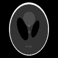
(a)	(b)	(c)

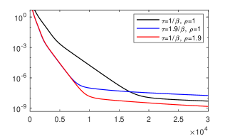
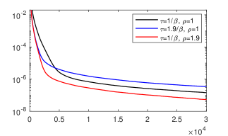
(d) $\|x^{(i)}-x^{\star}\|^{2}$ w.r.t. $i\geq 1$	(e) $\Psi(x^{(i)})-\Psi(x^{\star})$ w.r.t. $i\geq 1$

Figure 1: Image deblurring experiment: the goal is to estimate the reference image, which is the classical Shepp–Logan phantom (a), given the degraded image corrupted by blur and noise (b). The restored image (c) is the solution of a regularized least-squares problem of the form (4.1). The Loris–Verhoeven algorithm (5) is used with $\sigma=1/(8\tau)$, according to Theorem 4.2 and Theorem 4.3, since $\|L\|^{2}\leq 8$. The squared distance to the solution $x^{\star}$ and the decay of the objective function $\Psi$ along the iterations are shown in (d) and (e), respectively, for different values of $\tau$ and $\rho^{(i)}$ constant and equal to $1$ (no relaxation) or $1.9$ (overrelaxation). The benefit of overrelaxation (red curve), as allowed in Theorem 4.3, is clearly visible.

In Figure 1, we illustrate how overrelaxation can accelerate the Loris–Verhoeven algorithm when ${\color[rgb]{0,0.0,0.8}h}$ is quadratic. We consider the problem of image deblurring, which consists in restoring an image $y$ corrupted by Gaussian blur and Gaussian noise, shown in Figure 1 (b). We formulate deblurring as an optimization problem of the form (4.1); that is, we aim at minimizing $\Psi={\color[rgb]{0,0.0,0.8}h}+{\color[rgb]{0.65,0.0,0.0}g}\circ L$, where ${\color[rgb]{0,0.0,0.8}h}:x\mapsto{\textstyle\frac{1}{2}}\|Ax-y\|^{2}$ is a least-squares data-fidelity term, with $A$ the convolution with a lowpass filter ($\beta=\|A\|=1$), and ${\color[rgb]{0.65,0.0,0.0}g}\circ L$ is the “isotropic” total variation [114]: $L$ maps the image to the vector field made of all horizontal and vertical finite differences, and ${\color[rgb]{0.65,0.0,0.0}g}$ is $\lambda$ times the $l_{1,2}$ norm (see [29, 50] for details), where $\lambda=0.002$ is the regularization parameter. So, we use the Loris–Verhoeven algorithm to solve the problem; a solution $x^{\star}$ (which seems to be unique and is estimated by $x^{(i)}$ with $i=10^{6}$) is shown in Figure 1 (c). We can see from the plots of $\|x^{(i)}-x^{\star}\|^{2}$ and $\Psi(x^{(i)})$ that the choice $\tau=\frac{1}{\beta}$, $\sigma\tau\|L\|^{2}=1$, and $\rho^{(i)}=1.9$, as allowed by Theorem 4.3, speeds up the convergence in comparison with the standard choices allowed by Theorem 4.2.

4.1 The Primal-Dual Fixed-Point (PDFP) algorithm

Let us extend the problem (4.1) to

$$\operatorname*{minimize}_{x\in\mathcal{X}}\,{\color[rgb]{0,0.42,0}f(x)}+{\color[rgb]{0.65,0.0,0.0}g(Lx)}+{\color[rgb]{0,0.0,0.8}h(x)},$$ (4.36)

using the same assumptions as before in this section, with an additional function ${\color[rgb]{0,0.42,0}f}\in\Gamma_{0}(\mathcal{X})$. The dual problem is

$$\operatorname*{minimize}_{u\in\mathcal{U}}\,({\color[rgb]{0,0.42,0}f}+{\color[rgb]{0,0.0,0.8}h})^{*}(-L^{*}u)+{\color[rgb]{0.65,0.0,0.0}g^{*}(u)}.$$ (4.37)

Can we modify the Loris–Verhoeven algorithm to handle this extended problem? We will see one way to do this in section 8, with the PD3O algorithm. Meanwhile, let us extend the Loris–Verhoeven algorithm by keeping its primal-dual forward-backward structure. For this, we suppose that for any $\gamma>0$, the proximity operator of $\gamma{\color[rgb]{0,0.42,0}f}$ is affine; that is, there exist some self-adjoint, positive, bounded linear operator ${\color[rgb]{0,0.42,0}R_{\gamma}}$ on $\mathcal{X}$, with $\|{\color[rgb]{0,0.42,0}R_{\gamma}}\|\leq 1$, and some element $a_{\gamma}\in\mathcal{X}$, such that

$$\mathrm{prox}_{\gamma{\color[rgb]{0,0.42,0}f}}:x\in\mathcal{X}\mapsto{\color[rgb]{0,0.42,0}R_{\gamma}}x+a_{\gamma}.$$ (4.38)

We mention two cases of practical interest, where the proximity operator is affine. First, this is the case if ${\color[rgb]{0,0.42,0}f}$ is quadratic: ${\color[rgb]{0,0.42,0}f}:x\in\mathcal{X}\mapsto\frac{1}{2}\langle x,{\color[rgb]{0,0.42,0}Q^{\prime}}x\rangle+\langle x,c^{\prime}\rangle+t^{\prime}$ for some self-adjoint, positive, bounded linear operator ${\color[rgb]{0,0.42,0}Q^{\prime}}$, some $c^{\prime}\in\mathcal{X}$, and some $t^{\prime}\in\mathbb{R}$, with ${\color[rgb]{0,0.42,0}R_{\gamma}}=(\gamma{\color[rgb]{0,0.42,0}Q^{\prime}}+\mathrm{Id})^{-1}$ and $a_{\gamma}=-(\gamma{\color[rgb]{0,0.42,0}Q^{\prime}}+\mathrm{Id})^{-1}c^{\prime}$. Second, this is the case if ${\color[rgb]{0,0.42,0}f}$ is the indicator function of an affine subspace: ${\color[rgb]{0,0.42,0}f}:x\mapsto(0$ if $x\in\mathcal{A}$, $+\infty$ otherwise$)$, where $\mathcal{A}$ is a closed affine subspace of $\mathcal{X}$; for instance, $\mathcal{A}=\{x\in\mathcal{X}:Ax=y\}$ for some bounded linear operator $A$ and some element $y$ in the range of $A$; then $\mathrm{prox}_{\gamma{\color[rgb]{0,0.42,0}f}}$ is the projector onto $\mathcal{A}$, which does not depend on $\gamma$.

Let $\tau>0$ and $\sigma>0$. The extended Loris–Verhoeven iteration, written in implicit form, is

$$\left(\!\begin{array}[]{c}0\\ 0\\ \end{array}\!\right) \in\underbrace{\left(\begin{array}[]{c}{\color[rgb]{0,0.42,0}\partial f}(x^{(i+\frac{1}{2})})+L^{*}u^{(i+\frac{1}{2})}\\ -Lx^{(i+\frac{1}{2})}+({\color[rgb]{0.65,0.0,0.0}\partial g})^{-1}u^{(i+\frac{1}{2})}\\ \end{array}\right)}_{Mz^{(i+\frac{1}{2})}}$$ (4.43)

$$\quad\ +\underbrace{\left(\begin{array}[]{c}{\color[rgb]{0,0.0,0.8}\nabla h}(x^{(i)})\\ 0\\ \end{array}\right)}_{{\color[rgb]{0,0.0,0.8}C}z^{(i)}}+\underbrace{\left(\begin{array}[]{cc}\frac{1}{\tau}\mathrm{Id}&0\\ 0&\frac{1}{\sigma}\mathrm{Id}-\tau L{\color[rgb]{0,0.42,0}R_{\tau}}L^{*}\\ \end{array}\right)}_{P}\underbrace{\left(\begin{array}[]{c}x^{(i+\frac{1}{2})}-x^{(i)}\\ u^{(i+\frac{1}{2})}-u^{(i)}\\ \end{array}\right)}_{z^{(i+\frac{1}{2})}-z^{(i)}}.$$ (4.50)

This corresponds to the iteration:

$$\,\mbox{{PDFP iteration for \eqref{eq13e} and \eqref{eq21e}}: for }i=0,1,\ldots,$$

$$\left\lfloor\begin{array}[]{l}\tilde{x}^{(i)}=\mathrm{prox}_{\tau{\color[rgb]{0,0.42,0}f}}\big{(}x^{(i)}-\tau{\color[rgb]{0,0.0,0.8}\nabla h}(x^{(i)})-\tau L^{*}u^{(i)}\big{)}\\ u^{(i+\frac{1}{2})}=\mathrm{prox}_{\sigma{\color[rgb]{0.65,0.0,0.0}g^{*}}}\big{(}u^{(i)}+\sigma L\tilde{x}^{(i)}\big{)}\\ x^{(i+\frac{1}{2})}=\mathrm{prox}_{\tau{\color[rgb]{0,0.42,0}f}}\big{(}x^{(i)}-\tau{\color[rgb]{0,0.0,0.8}\nabla h}(x^{(i)})-\tau L^{*}u^{(i+\frac{1}{2})}\big{)}\\ x^{(i+1)}=x^{(i)}+\rho^{(i)}(x^{(i+\frac{1}{2})}-x^{(i)})\\ u^{(i+1)}=u^{(i)}+\rho^{(i)}(u^{(i+\frac{1}{2})}-u^{(i)}).\end{array}\right.$$ (4.56)

This algorithm has been analyzed by Chen et al. [34] and called the Primal-Dual Fixed-Point (PDFP) algorithm, so we give it the same name.

Since the algorithm has the structure of a primal-dual forward-backward algorithm, we can, again, invoke Theorem 3.2, and we obtain:

Theorem 4.4 (PDFP algorithm (4.1), affine $\mathrm{prox}_{{\color[rgb]{0,0.42,0}f}}$ case).

Suppose that $\mathrm{prox}_{{\color[rgb]{0,0.42,0}f}}$ is affine. Let $x^{(0)}\in\mathcal{X}$ and $u^{(0)}\in\mathcal{U}$. Let $\tau\in(0,2/\beta)$ and $\sigma>0$ be such that $\sigma\tau\|L{\color[rgb]{0,0.42,0}R_{\tau}}L^{*}\|<1$. Set $\delta=2-\tau\beta/2$. Let $(\rho^{(i)})_{i\in\mathbb{N}}$ be a sequence in $[0,\delta]$ such that $\sum_{i\in\mathbb{N}}\rho^{(i)}(\delta-\rho^{(i)})=+\infty$. Then the sequences $(x^{(i)})_{i\in\mathbb{N}}$ and $(u^{(i)})_{i\in\mathbb{N}}$ defined by the iteration (4.1) converge weakly to a solution of (4.36) and a solution of (4.37), respectively.

We note that $\|L{\color[rgb]{0,0.42,0}R_{\tau}}L^{*}\|\leq\|L\|^{2}$, so if $\sigma\tau\|L\|^{2}<1$, then $\sigma\tau\|L{\color[rgb]{0,0.42,0}R_{\tau}}L^{*}\|<1$.

Chen et al. have proved convergence of the PDFP algorithm with any function ${\color[rgb]{0,0.42,0}f}$, not only in the affine proximity operator case, as follows [34, Theorem 3.1]:

Theorem 4.5 (PDFP algorithm (4.1), general case).

Suppose that $\mathcal{X}$ and $\mathcal{U}$ are of finite dimension. Let $x^{(0)}\in\mathcal{X}$ and $u^{(0)}\in\mathcal{U}$. Let $\tau\in(0,2/\beta)$ and $\sigma>0$ be such that $\sigma\tau\|L\|^{2}<1$. Set $\rho^{(i)}=1$ for every $i\in\mathbb{N}$. Then the sequences $(x^{(i)})_{i\in\mathbb{N}}$ and $(u^{(i)})_{i\in\mathbb{N}}$ defined by the iteration (4.1) converge to a solution of (4.36) and a solution of (4.37), respectively.

It remains an open question whether the PDFP algorithm can be relaxed like in Theorem 4.4 for an arbitrary ${\color[rgb]{0,0.42,0}f}$.

We can check that when ${\color[rgb]{0,0.0,0.8}h}=\frac{\beta}{2}\|\cdot\|^{2}$, it is equivalent to applying the Loris–Verhoeven algorithm to minimize ${\color[rgb]{0.65,0.0,0.0}g}\circ L+{\color[rgb]{0,0.0,0.8}h}$ or to applying the PDFP algorithm to minimize ${\color[rgb]{0,0.42,0}f}+{\color[rgb]{0.65,0.0,0.0}g}\circ L$, with ${\color[rgb]{0,0.42,0}f}=\frac{\beta}{2}\|\cdot\|^{2}$. Indeed, in the latter case, let $\tau^{\prime}>0$ and $\sigma>0$ be the parameters of the PDFP algorithm. Set $\tau=\frac{\tau^{\prime}}{1+\tau^{\prime}\beta}$. We have $\mathrm{prox}_{\tau^{\prime}{\color[rgb]{0,0.42,0}f}}:x\in\mathcal{X}\mapsto\frac{1}{1+\tau^{\prime}\beta}x$, which is linear. Then the PDFP algorithm (4.1) becomes:

$$\,\mbox{{PDFP iteration}: for }i=0,1,\ldots,$$

$$\left\lfloor\begin{array}[]{l}u^{(i+\frac{1}{2})}=\mathrm{prox}_{\sigma{\color[rgb]{0.65,0.0,0.0}g^{*}}}\Big{(}u^{(i)}+\frac{\sigma}{1+\tau^{\prime}\beta}L\big{(}x^{(i)}-\tau^{\prime}L^{*}u^{(i)}\big{)}\Big{)}\\ \hphantom{u^{(i+\frac{1}{2})}}=\mathrm{prox}_{\sigma{\color[rgb]{0.65,0.0,0.0}g^{*}}}\Big{(}u^{(i)}+\sigma L\big{(}x^{(i)}-\tau{\color[rgb]{0,0.0,0.8}\nabla h}(x^{(i)})-\tau L^{*}u^{(i)}\big{)}\Big{)}\\ x^{(i+\frac{1}{2})}=\frac{1}{1+\tau^{\prime}\beta}\big{(}x^{(i)}-\tau^{\prime}L^{*}u^{(i+\frac{1}{2})}\big{)}\\ \hphantom{x^{(i+\frac{1}{2})}}=x^{(i)}-\tau{\color[rgb]{0,0.0,0.8}\nabla h}(x^{(i)})-\tau L^{*}u^{(i+\frac{1}{2})}\\ x^{(i+1)}=x^{(i)}+\rho^{(i)}(x^{(i+\frac{1}{2})}-x^{(i)})\\ u^{(i+1)}=u^{(i)}+\rho^{(i)}(u^{(i+\frac{1}{2})}-u^{(i)}),\end{array}\right.$$ (4.63)

and we recover the Loris–Verhoeven algorithm (4) applied to minimize ${\color[rgb]{0.65,0.0,0.0}g}\circ L+{\color[rgb]{0,0.0,0.8}h}$, with parameters $\tau$ and $\sigma$. The conditions for convergence from the PDFP interpretation are $\tau<1/\beta$, $\sigma\tau\|L\|^{2}<1$, and $\delta=2$, so that we do not gain anything in comparison with Theorem 4.3.

5 The Chambolle–Pock and the Douglas–Rachford Algorithms

We now consider a problem similar to (4.1), but this time we want to make use of the proximity operators of the two functions. So, let $\mathcal{X}$ and $\mathcal{U}$ be two real Hilbert spaces. Let ${\color[rgb]{0,0.42,0}f}\in\Gamma_{0}(\mathcal{X})$ and ${\color[rgb]{0.65,0.0,0.0}g}\in\Gamma_{0}(\mathcal{U})$. Let $L:\mathcal{X}\rightarrow\mathcal{U}$ be a nonzero bounded linear operator. We want to

$$\operatorname*{minimize}_{x\in\mathcal{X}}\,{\color[rgb]{0,0.42,0}f(x)}+{\color[rgb]{0.65,0.0,0.0}g(Lx)}.$$ (5.1)

The corresponding monotone inclusion is

$$0\in{\color[rgb]{0,0.42,0}\partial f}(x)+L^{*}{\color[rgb]{0.65,0.0,0.0}\partial g}(Lx).$$ (5.2)

Again, to bypass the annoying operator $L$, we introduce an auxiliary variable $u\in{\color[rgb]{0.65,0.0,0.0}\partial g}(Lx)$, which will be called the dual variable, so that the problem now consists in finding $x\in\mathcal{X}$ and $u\in\mathcal{U}$ such that

$$\left\{\begin{array}[]{l}u\in{\color[rgb]{0.65,0.0,0.0}\partial g}(Lx)\\ 0\in L^{*}u+{\color[rgb]{0,0.42,0}\partial f}(x)\end{array}\right..$$ (5.3)

Let us define the dual convex optimization problem associated to the primal problem (5.1):

$$\operatorname*{minimize}_{u\in\mathcal{U}}\,{\color[rgb]{0,0.42,0}f^{*}(-L^{*}u)}+{\color[rgb]{0.65,0.0,0.0}g^{*}(u)}.$$ (5.4)

If a pair $(x,u)\in\mathcal{X}\times\mathcal{U}$ is a solution to (5.3), then $x$ is a solution to (5.1) and $u$ is a solution to (5.4).

To solve the primal and dual problems (5.1) and (5.4) jointly, Chambolle and Pock [27] proposed the following algorithms (without relaxation); see also Esser et al. [65] and Zhang et al. [136]:

$$\,\mbox{{Chambolle--Pock iteration, form I, for \eqref{eq22} and \eqref{eq23}}: for }i=0,1,\ldots,$$

$$\left\lfloor\begin{array}[]{l}x^{(i+\frac{1}{2})}=\mathrm{prox}_{\tau{\color[rgb]{0,0.42,0}f}}\big{(}x^{(i)}-\tau L^{*}u^{(i)}\big{)}\\ u^{(i+\frac{1}{2})}=\mathrm{prox}_{\sigma{\color[rgb]{0.65,0.0,0.0}g^{*}}}\big{(}u^{(i)}+\sigma L(2x^{(i+\frac{1}{2})}-x^{(i)})\big{)}\\ x^{(i+1)}=x^{(i)}+\rho^{(i)}(x^{(i+\frac{1}{2})}-x^{(i)})\\ u^{(i+1)}=u^{(i)}+\rho^{(i)}(u^{(i+\frac{1}{2})}-u^{(i)}).\end{array}\right.$$ (5.9)

Chambolle–Pock iteration, form II, for (5.1) and (5.4):

$$\,\mbox{for }i=0,1,\ldots,$$

$$\left\lfloor\begin{array}[]{l}u^{(i+\frac{1}{2})}=\mathrm{prox}_{\sigma{\color[rgb]{0.65,0.0,0.0}g^{*}}}\big{(}u^{(i)}+\sigma Lx^{(i)}\big{)}\\ x^{(i+\frac{1}{2})}=\mathrm{prox}_{\tau{\color[rgb]{0,0.42,0}f}}\big{(}x^{(i)}-\tau L^{*}(2u^{(i+\frac{1}{2})}-u^{(i)})\big{)}\\ u^{(i+1)}=u^{(i)}+\rho^{(i)}(u^{(i+\frac{1}{2})}-u^{(i)})\\ x^{(i+1)}=x^{(i)}+\rho^{(i)}(x^{(i+\frac{1}{2})}-x^{(i)}).\end{array}\right.$$ (5.14)

We note that the Chambolle–Pock algorithm is self-dual: if we apply the Chambolle–Pock iteration form I to the problem (5.4) to minimize ${\color[rgb]{0,0.42,0}\tilde{f}}+{\color[rgb]{0.65,0.0,0.0}\tilde{g}}\circ\tilde{L}$ with ${\color[rgb]{0,0.42,0}\tilde{f}}={\color[rgb]{0.65,0.0,0.0}g^{*}}$, ${\color[rgb]{0.65,0.0,0.0}\tilde{g}}={\color[rgb]{0,0.42,0}f^{*}}$, $\tilde{L}=-L^{*}$, and the roles of $x$ and $u$ are switched, as are the roles of $\tau$ and $\sigma$, we obtain exactly the Chambolle–Pock iteration form II.

Chambolle and Pock proved the convergence in the finite-dimensional case, assuming that $\tau\sigma\|L\|^{2}<1$ and $\rho^{(i)}=1$ [27]. The convergence was proved in a different way by He and Yuan, with a constant relaxation parameter $\rho^{(i)}=\rho\in(0,2)$ and the other hypotheses the same [81]; indeed, they observed that the Chambolle–Pock algorithm is a primal-dual proximal point algorithm to find a primal-dual pair $z=(x,u)$ in $\mathcal{Z}=\mathcal{X}\times\mathcal{U}$, a solution to the monotone inclusion

$$\left(\begin{array}[]{c}0\\ 0\end{array}\right)\in\underbrace{\left(\begin{array}[]{c}{\color[rgb]{0,0.42,0}\partial f}(x)+L^{*}u\\ -Lx+({\color[rgb]{0.65,0.0,0.0}\partial g})^{-1}u\end{array}\right)}_{Mz}.$$ (5.15)

The operator $M:\mathcal{Z}\rightarrow 2^{\mathcal{Z}},(x,u)\mapsto({\color[rgb]{0,0.42,0}\partial f}(x)+L^{*}u,-Lx+({\color[rgb]{0.65,0.0,0.0}\partial g})^{-1}u)$ is maximally monotone [7, Proposition 26.32 (iii)]. Then one can observe that the Chambolle–Pock iteration form I satisfies

$$\left(\begin{array}[]{c}0\\ 0\\ \end{array}\right)\in\underbrace{\left(\begin{array}[]{c}{\color[rgb]{0,0.42,0}\partial f}(x^{(i+\frac{1}{2})})+L^{*}u^{(i+\frac{1}{2})}\\ -Lx^{(i+\frac{1}{2})}+({\color[rgb]{0.65,0.0,0.0}\partial g})^{-1}u^{(i+\frac{1}{2})}\\ \end{array}\right)}_{Mz^{(i+\frac{1}{2})}}+\underbrace{\left(\begin{array}[]{cc}\frac{1}{\tau}\mathrm{Id}&-L^{*}\\ -L&\frac{1}{\sigma}\mathrm{Id}\\ \end{array}\right)}_{P}\underbrace{\left(\begin{array}[]{c}x^{(i+\frac{1}{2})}-x^{(i)}\\ u^{(i+\frac{1}{2})}-u^{(i)}\\ \end{array}\right)}_{z^{(i+\frac{1}{2})}-z^{(i)}}.$$ (5.16)

The Chambolle–Pock iteration form II satisfies the same primal-dual inclusion, but with $-L$ replaced by $L$ in $P$.

Thus, the Chambolle–Pock iteration is a preconditioned primal-dual proximal point algorithm and, as a consequence of Theorem 3.3, we have [48, Theorem 3.2]:

Theorem 5.1 (Chambolle–Pock algorithm (5) or (5)).

Let $x^{(0)}\in\mathcal{X}$ and $u^{(0)}\in\mathcal{U}$. Let $\tau>0$ and $\sigma>0$ be such that $\sigma\tau\|L\|^{2}<1$. Let $(\rho^{(i)})_{i\in\mathbb{N}}$ be a sequence in $[0,2]$ such that $\sum_{i\in\mathbb{N}}\rho^{(i)}(2-\rho^{(i)})=+\infty$. Then the sequences $(x^{(i)})_{i\in\mathbb{N}}$ and $(u^{(i)})_{i\in\mathbb{N}}$, defined either by the iteration (5) or by the iteration (5), converge weakly to a solution of (5.1) and a solution of (5.4), respectively.

In addition, the first author proved that in the finite-dimensional setting, one can set $\sigma\tau\|L\|^{2}=1$ [48, Theorem 3.3], see also O’Connor and Vandenberghe [97] for another proof and [15] for a discussion in a generalized setting. If we apply Theorem 6.2 below with $K=\mathrm{Id}$ and $\eta=1/\tau$, we obtain:

Theorem 5.2 (Chambolle–Pock algorithm (5) or (5)).

Let $x^{(0)}\in\mathcal{X}$ and $u^{(0)}\in\mathcal{U}$. Let $\tau>0$ and $\sigma>0$ be such that $\sigma\tau\|L\|^{2}\leq 1$. Let $(\rho^{(i)})_{i\in\mathbb{N}}$ be a sequence in $[0,2]$ such that $\sum_{i\in\mathbb{N}}\rho^{(i)}(2-\rho^{(i)})=+\infty$. Then the sequences $(x^{(i)})_{i\in\mathbb{N}}$ and $(u^{(i)})_{i\in\mathbb{N}}$, defined either by the iteration (5) or by the iteration (5), converge weakly to a solution of (5.1) and a solution of (5.4), respectively.

The difference between Theorem 5.1 and Theorem 5.2 is that $\sigma\tau\|L\|^{2}=1$ is allowed in the latter. This is a significant improvement: in practice, one can set $\sigma=1/(\tau\|L\|^{2})$ in the algorithms and have only one parameter remaining, namely $\tau$, to tune.

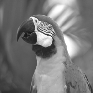
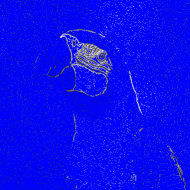
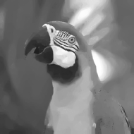
(a)	(b)	(c)

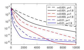
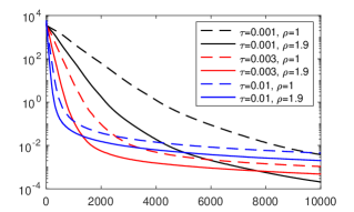
(d) $\|x^{(i)}-x^{\star}\|^{2}$ w.r.t. $i\geq 1$	(e) $\Psi(x^{(i)})-\Psi(x^{\star})$ w.r.t. $i\geq 1$

Figure 2: Image inpainting experiment: the goal is to estimate the reference image (a) given only a subset (8%) of its pixel values (b), with the missing values shown in blue. The reconstructed image (c) is the solution of the convex optimization problem of the form (5.1) of minimizing the total variation, while keeping the available pixel values. The Chambolle–Pock algorithm (5) is used with $\sigma=1/(8\tau)$, according to Theorem 5.2, since $\|L\|^{2}\leq 8$. The squared distance to the solution $x^{\star}$ and the decay of the objective function $\Psi$ along the iterations are shown in (d) and (e), respectively, for three different values of $\tau$ and $\rho^{(i)}$ constant and equal to $1$ (no relaxation) or $1.9$ (overrelaxation). The benefit of overrelaxation is clearly visible.

In Figure 2, we illustrate how overrelaxation can accelerate the Chambolle–Pock algorithm. We consider the problem of image inpainting, which consists in estimating missing pixel values of an image. We formulate inpainting as an optimization problem of the form (5.1); that is, we aim at minimizing $\Psi={\color[rgb]{0,0.42,0}f}+{\color[rgb]{0.65,0.0,0.0}g}\circ L$, where ${\color[rgb]{0,0.42,0}f}$ is the indicator function of the affine subspace of images having the prescribed pixel values, and ${\color[rgb]{0.65,0.0,0.0}g}\circ L$ is the “isotropic” total variation [114, 29, 50]. So, we use the Chambolle–Pock algorithm to solve the problem; a solution $x^{\star}$ (which seems to be unique and is estimated by $x^{(i)}$ with $i=10^{6}$) is shown in Figure 2 (c). We can see from the plots of $\|x^{(i)}-x^{\star}\|^{2}$ and $\Psi(x^{(i)})-\Psi(x^{\star})={\color[rgb]{0.65,0.0,0.0}g}(Lx^{(i)})-{\color[rgb]{0.65,0.0,0.0}g}(Lx^{\star})$ (since ${\color[rgb]{0,0.42,0}f}(x^{(i)})=0$ for every $i$) that the best value of $\tau$ depends on the desired accuracy or number of iterations: $\tau=0.01$ is better after $10^{3}$ iterations, whereas a smaller value is better after $10^{4}$ iterations. In any case, $\rho^{(i)}=1.9$ significantly speeds up the convergence, in comparison with $\rho^{(i)}=1$.

5.1 The Proximal Method of Multipliers

Let $\mathcal{X}$ and $\mathcal{U}$ be two real Hilbert spaces. Let ${\color[rgb]{0.65,0.0,0.0}g}\in\Gamma_{0}(\mathcal{U})$, $c\in\mathcal{X}$, and let $L:\mathcal{X}\rightarrow\mathcal{U}$ be a bounded linear operator. We consider the problem

$$\operatorname*{minimize}_{x\in\mathcal{X}}\,{\color[rgb]{0.65,0.0,0.0}g(Lx)}+\langle x,c\rangle$$ (5.17)

and the dual problem

$$\operatorname*{minimize}_{u\in\mathcal{U}}\,{\color[rgb]{0.65,0.0,0.0}g^{*}(u)}\quad\mbox{s.t.}\quad L^{*}u+c=0.$$ (5.18)

We can view the term $\langle x,c\rangle$ as a smooth function ${\color[rgb]{0,0.0,0.8}h}$ with constant gradient ${\color[rgb]{0,0.0,0.8}\nabla h}=c$ and apply the Loris–Verhoeven algorithm. Thus, let $\tau>0$ and $\sigma>0$, let $x^{(0)}\in\mathcal{X}$ and $u^{(0)}\in\mathcal{U}$, and let $(\rho^{(i)})_{i\in\mathbb{N}}$ be a sequence of relaxation parameters. The iteration is (we change the name of the variable $x$ to $s$):

$$\,\mbox{{Loris--Verhoeven iteration for \eqref{eqpalm1} and \eqref{eqpalm2}}: for }i=0,1,\ldots,$$

$$\left\lfloor\begin{array}[]{l}u^{(i+\frac{1}{2})}=\mathrm{prox}_{\sigma{\color[rgb]{0.65,0.0,0.0}g^{*}}}\big{(}u^{(i)}+\sigma L(s^{(i)}-\tau L^{*}u^{(i)}-\tau c)\big{)}\\ s^{(i+1)}=s^{(i)}-\rho^{(i)}\tau(L^{*}u^{(i+\frac{1}{2})}+c)\\ u^{(i+1)}=u^{(i)}+\rho^{(i)}(u^{(i+\frac{1}{2})}-u^{(i)}).\end{array}\right.$$ (5.22)

Each iteration of the algorithm satisfies the inclusion

$$\left(\!\begin{array}[]{c}0\\ 0\\ \end{array}\!\right)\in\left(\begin{array}[]{c}c+L^{*}u^{(i+\frac{1}{2})}\\ -Ls^{(i+\frac{1}{2})}+({\color[rgb]{0.65,0.0,0.0}\partial g})^{-1}u^{(i+\frac{1}{2})}\\ \end{array}\right)+\left(\begin{array}[]{cc}\frac{1}{\tau}\mathrm{Id}&0\\ 0&\frac{1}{\sigma}\mathrm{Id}-\tau LL^{*}\\ \end{array}\right)\left(\begin{array}[]{c}s^{(i+\frac{1}{2})}-s^{(i)}\\ u^{(i+\frac{1}{2})}-u^{(i)}\\ \end{array}\right)\!.$$ (5.23)

Since the algorithm has the structure of a proximal point algorithm, we can apply Theorem 3.3 and obtain convergence under the condition $\sigma\tau\|L\|^{2}<1$.

An alternative is to see the term $\langle x,c\rangle$ as a function ${\color[rgb]{0,0.42,0}f}$ with proximity operator $\mathrm{prox}_{\tau{\color[rgb]{0,0.42,0}f}}:x\mapsto x-\tau c$. Thus, we can solve (5.17) and (5.18) by applying the Chambolle–Pock algorithm (we change the name of its variable $x^{(i+\frac{1}{2})}$ to $s^{(i)}$):

Chambolle–Pock iteration, form I, for (5.17) and (5.18):

$$\,\mbox{for }i=0,1,\ldots,$$

$$\left\lfloor\begin{array}[]{l}s^{(i)}=x^{(i)}-\tau L^{*}u^{(i)}-\tau c\\ u^{(i+\frac{1}{2})}=\mathrm{prox}_{\sigma{\color[rgb]{0.65,0.0,0.0}g^{*}}}\big{(}u^{(i)}+\sigma L(2s^{(i)}-x^{(i)})\big{)}\\ \hphantom{u^{(i+\frac{1}{2})}}{}=\mathrm{prox}_{\sigma{\color[rgb]{0.65,0.0,0.0}g^{*}}}\big{(}u^{(i)}+\sigma L(s^{(i)}-\tau L^{*}u^{(i)}-\tau c)\big{)}\\ x^{(i+1)}=x^{(i)}+\rho^{(i)}(s^{(i)}-x^{(i)})\\ \hphantom{x^{(i+1)}}{}=x^{(i)}-\rho^{(i)}\tau(L^{*}u^{(i)}+c)\\ u^{(i+1)}=u^{(i)}+\rho^{(i)}(u^{(i+\frac{1}{2})}-u^{(i)}).\end{array}\right.$$ (5.30)

We can discard the variable $x$ and the iteration becomes:

$$\left\lfloor\begin{array}[]{l}u^{(i+\frac{1}{2})}=\mathrm{prox}_{\sigma{\color[rgb]{0.65,0.0,0.0}g^{*}}}\big{(}u^{(i)}+\sigma L(s^{(i)}-\tau L^{*}u^{(i)}-\tau c)\big{)}\\ s^{(i+1)}=s^{(i)}-\rho^{(i)}\tau\big{(}L^{*}u^{(i+\frac{1}{2})}+c\big{)}\\ u^{(i+1)}=u^{(i)}+\rho^{(i)}(u^{(i+\frac{1}{2})}-u^{(i)}),\end{array}\right.$$ (5.34)

and we exactly recover the iteration (5.1). Therefore, the Loris–Verhoeven algorithm and the Chambolle–Pock algorithm are the same for the specific problems (5.17) and (5.18); we call this algorithm the Proximal Method of Multipliers [112].

Furthermore, the form (5.1) provides us with a compact form of the algorithm:

$$\,\mbox{{Proximal Method of Multipliers for \eqref{eqpalm1} and \eqref{eqpalm2}}: for }i=0,1,\ldots,$$

$$\left\lfloor\begin{array}[]{l}a^{(i)}=L^{*}u^{(i)}+c\\ u^{(i+1)}=u^{(i)}+\rho^{(i)}\Big{(}\mathrm{prox}_{\sigma{\color[rgb]{0.65,0.0,0.0}g^{*}}}\big{(}u^{(i)}+\sigma L(x^{(i)}-2\tau a^{(i)})\big{)}-u^{(i)}\Big{)}\\ x^{(i+1)}=x^{(i)}-\rho^{(i)}\tau a^{(i)},\end{array}\right.$$ (5.38)

and since the two updates are independent, they can be performed in parallel.

Theorem 5.2 yields:

Theorem 5.3 (Proximal Method of Multipliers (5.1)).

Let $x^{(0)}\in\mathcal{X}$ and $u^{(0)}\in\mathcal{U}$. Let $\tau>0$ and $\sigma>0$ be such that $\sigma\tau\|L\|^{2}\leq 1$. Let $(\rho^{(i)})_{i\in\mathbb{N}}$ be a sequence in $[0,2]$ such that $\sum_{i\in\mathbb{N}}\rho^{(i)}(2-\rho^{(i)})=+\infty$. Then the sequences $(x^{(i)})_{i\in\mathbb{N}}$ and $(u^{(i)})_{i\in\mathbb{N}}$ defined by the iteration (5.1) converge weakly to a solution of (5.17) and a solution of (5.18), respectively.

We can also apply the form II of the Chambolle–Pock algorithm, with the same convergence properties as in Theorem 5.3:

Chambolle–Pock iteration, form II, for (5.17) and (5.18):

$$\,\mbox{for }i=0,1,\ldots,$$

$$\left\lfloor\begin{array}[]{l}u^{(i+\frac{1}{2})}=\mathrm{prox}_{\sigma{\color[rgb]{0.65,0.0,0.0}g^{*}}}\big{(}u^{(i)}+\sigma Lx^{(i)}\big{)}\\ x^{(i+1)}=x^{(i)}-\rho^{(i)}\tau\big{(}L^{*}(2u^{(i+\frac{1}{2})}-u^{(i)})+c\big{)}\\ u^{(i+1)}=u^{(i)}+\rho^{(i)}(u^{(i+\frac{1}{2})}-u^{(i)}).\end{array}\right.$$ (5.42)

5.2 The Douglas–Rachford algorithm

Let us consider the particular case of the problem (5.1) when $\mathcal{X}=\mathcal{U}$ and $L=\mathrm{Id}$. The problem becomes

$$\operatorname*{minimize}_{x\in\mathcal{X}}\,{\color[rgb]{0,0.42,0}f(x)}+{\color[rgb]{0.65,0.0,0.0}g(x)}.$$ (5.43)

By setting $\sigma=1/\tau$ in the Chambolle–Pock algorithm, we recover the Douglas–Rachford algorithm [87, 59, 36, 126] as a particular case:

$$\,\mbox{{Douglas--Rachford iteration for \eqref{eqpdr}}: for }i=0,1,\ldots,$$

$$\left\lfloor\begin{array}[]{l}x^{(i+\frac{1}{2})}=\mathrm{prox}_{\tau{\color[rgb]{0,0.42,0}f}}\big{(}x^{(i)}-\tau u^{(i)}\big{)}\\ u^{(i+\frac{1}{2})}=\mathrm{prox}_{{\color[rgb]{0.65,0.0,0.0}g^{*}}/\tau}\big{(}u^{(i)}+(2x^{(i+\frac{1}{2})}-x^{(i)})/\tau\big{)}\\ x^{(i+1)}=x^{(i)}+\rho^{(i)}(x^{(i+\frac{1}{2})}-x^{(i)})\\ u^{(i+1)}=u^{(i)}+\rho^{(i)}(u^{(i+\frac{1}{2})}-u^{(i)}).\end{array}\right.$$ (5.48)

Note that the Douglas–Rachford algorithm is not a primal-dual proximal point algorithm since the operator $P$ in (5.16) is no longer strongly positive. So, its weak convergence, which is not strong in general [21], is difficult to establish; it was only shown in 2011 by Svaiter [126]. Let us have a quick look at the structure of the Douglas–Rachford algorithm. First, we define the auxiliary variable

$$s^{(i)}=x^{(i)}-\tau u^{(i)}.$$ (5.49)

The Douglas–Rachford iteration depends only on this concatenated variable, not on the full pair $(x^{(i)},u^{(i)})$, and we can rewrite it as:

$$\,\mbox{{Douglas--Rachford iteration for \eqref{eqpdr}}: for }i=0,1,\ldots,$$

$$\left\lfloor\begin{array}[]{l}x^{(i+\frac{1}{2})}=\mathrm{prox}_{\tau{\color[rgb]{0,0.42,0}f}}(s^{(i)})\\ u^{(i+\frac{1}{2})}=\mathrm{prox}_{{\color[rgb]{0.65,0.0,0.0}g^{*}}/\tau}\big{(}(2x^{(i+\frac{1}{2})}-s^{(i)})/\tau\big{)}\\ s^{(i+1)}=s^{(i)}+\rho^{(i)}(x^{(i+\frac{1}{2})}-\tau u^{(i+\frac{1}{2})}-s^{(i)}),\end{array}\right.$$ (5.53)

or, equivalently,

$$\,\mbox{{Douglas--Rachford iteration for \eqref{eqpdr}}: for }i=0,1,\ldots,$$

$$\left\lfloor\begin{array}[]{l}x^{(i+\frac{1}{2})}=\mathrm{prox}_{\tau{\color[rgb]{0,0.42,0}f}}(s^{(i)})\\ s^{(i+1)}=s^{(i)}+\rho^{(i)}\big{(}\mathrm{prox}_{\tau{\color[rgb]{0.65,0.0,0.0}g}}(2x^{(i+\frac{1}{2})}-s^{(i)})-x^{(i+\frac{1}{2})}\big{)}.\end{array}\right.$$ (5.56)

Or, keeping only the variable $s$:

$$\textstyle\left\lfloor\begin{array}[]{l}s^{(i+\frac{1}{2})}=\big{(}\frac{1}{2}(2\mathrm{prox}_{\tau{\color[rgb]{0.65,0.0,0.0}g}}-\mathrm{Id})(2\mathrm{prox}_{\tau{\color[rgb]{0,0.42,0}f}}-\mathrm{Id})+\frac{1}{2}\mathrm{Id}\big{)}s^{(i)}\\ s^{(i+1)}=s^{(i)}+\rho^{(i)}(s^{(i+\frac{1}{2})}-s^{(i)}).\end{array}\right.$$ (5.57)

Since the operator mapping $s^{(i)}$ to $s^{(i+\frac{1}{2})}$ is firmly nonexpansive, $(s^{(i)})_{i\in\mathbb{N}}$ converges weakly, after the Krasnosel’skiĭ–Mann theorem, for every $\tau>0$ and sequence $(\rho^{(i)})_{i\in\mathbb{N}}$ in $[0,2]$ such that $\sum_{i\in\mathbb{N}}\rho^{(i)}(2-\rho^{(i)})=+\infty$. But in infinite dimension, one cannot deduce that $(x^{(i+\frac{1}{2})})_{i\in\mathbb{N}}$ converges. In finite dimension, however, the proximity operator is continuous, so that one can indeed conclude that $(x^{(i+\frac{1}{2})})_{i\in\mathbb{N}}$ converges to some minimizer of ${\color[rgb]{0,0.42,0}f}+{\color[rgb]{0.65,0.0,0.0}g}$.

As an application of Corollary 28.3 in [7], which proves weak convergence using fine properties of the operators, we have:

Theorem 5.4 (Douglas–Rachford algorithm (5.2)).

Let $s^{(0)}\in\mathcal{X}$. Let $\tau>0$ and let $(\rho^{(i)})_{i\in\mathbb{N}}$ be a sequence in $[0,2]$ such that $\sum_{i\in\mathbb{N}}\rho^{(i)}(2-\rho^{(i)})=+\infty$. Then the sequence $(x^{(i+\frac{1}{2})})_{i\in\mathbb{N}}$ defined by the iteration (5.2) converges weakly to a solution of (5.43).

Note that it would be misleading to state Theorem 5.4 by invoking Theorem 5.2, since Theorem 5.2 is itself based on the convergence result of the Douglas–Rachford algorithm [7, Corollary 28.3]. In other words, weak convergence of the Douglas–Rachford algorithm is the fundamental result from which we deduce weak convergence of the Chambolle–Pock algorithm, which generalizes it.

As mentioned in [41], the limit case of the Douglas–Rachford algorithm with $\rho^{(i)}=2$ is the Peaceman–Rachford algorithm [87, 59, 36]. But in that case, the operator $T=(2\mathrm{prox}_{\tau{\color[rgb]{0.65,0.0,0.0}g}}-\mathrm{Id})(2\mathrm{prox}_{\tau{\color[rgb]{0,0.42,0}f}}-\mathrm{Id})$ mapping $s^{(i)}$ to $s^{(i+1)}$ is merely nonexpansive and not averaged. For instance, with ${\color[rgb]{0,0.42,0}f}=0$ and ${\color[rgb]{0.65,0.0,0.0}g}:x\mapsto(0\$if$\ x=0,\ +\infty\$otherwise$)$, so that the minimizer of ${\color[rgb]{0,0.42,0}f}+{\color[rgb]{0.65,0.0,0.0}g}$ is $0$, we have $T=-\mathrm{Id}$ and the iteration $x^{(i+\frac{1}{2})}=s^{(i)}$, $s^{(i+1)}=-s^{(i)}$, which cycles and does not converge if $s^{(0)}\neq 0$. This shows the tightness of the Krasnosel’skiĭ–Mann theorem. The Peaceman–Rachford algorithm converges under additional assumptions, for instance if ${\color[rgb]{0,0.42,0}f}$ is strictly convex and real-valued [38].

Let us show that, like the Chambolle–Pock algorithm, the Douglas–Rachford algorithm is self-dual [58, Lemma 3.6][134]: it is equivalent to apply it to the primal problem (5.43) or to the dual problem:

$$\operatorname*{minimize}_{u\in\mathcal{X}}\,{\color[rgb]{0,0.42,0}f^{*}(-u)}+{\color[rgb]{0.65,0.0,0.0}g^{*}(u)}.$$ (5.58)

Using the Moreau identity (2.24) and starting from the form (5.2), we can write the Douglas–Rachford iteration as:

$$\left\lfloor\begin{array}[]{l}v^{(i+\frac{1}{2})}=\mathrm{prox}_{{\color[rgb]{0,0.42,0}f^{*}(-\cdot)}/\tau}\big{(}u^{(i)}-\frac{1}{\tau}x^{(i)}\big{)}\\ x^{(i+\frac{1}{2})}=x^{(i)}-\tau(u^{(i)}-v^{(i+\frac{1}{2})})\\ u^{(i+\frac{1}{2})}=\mathrm{prox}_{{\color[rgb]{0.65,0.0,0.0}g^{*}}/\tau}\big{(}v^{(i+\frac{1}{2})}+\frac{1}{\tau}x^{(i+\frac{1}{2})}\big{)}\\ x^{(i+1)}=x^{(i)}+\rho^{(i)}(x^{(i+\frac{1}{2})}-x^{(i)})\\ u^{(i+1)}=u^{(i)}+\rho^{(i)}(u^{(i+\frac{1}{2})}-u^{(i)}).\end{array}\right.$$ (5.64)

If we introduce the variable $\tilde{s}^{(i)}=\frac{-1}{\tau}s^{(i)}=u^{(i)}-\frac{1}{\tau}x^{(i)}$, we can rewrite the iteration as:

$$\left\lfloor\begin{array}[]{l}v^{(i+\frac{1}{2})}=\mathrm{prox}_{{\color[rgb]{0,0.42,0}f^{*}(-\cdot)}/\tau}(\tilde{s}^{(i)})\\ x^{(i+\frac{1}{2})}=x^{(i)}-\tau(u^{(i)}-v^{(i+\frac{1}{2})})\\ u^{(i+\frac{1}{2})}=\mathrm{prox}_{{\color[rgb]{0.65,0.0,0.0}g^{*}}/\tau}\big{(}2v^{(i+\frac{1}{2})}-\tilde{s}^{(i)}\big{)}\\ x^{(i+1)}=x^{(i)}+\rho^{(i)}(x^{(i+\frac{1}{2})}-x^{(i)})\\ u^{(i+1)}=u^{(i)}+\rho^{(i)}(u^{(i+\frac{1}{2})}-u^{(i)})\\ \tilde{s}^{(i+1)}=u^{(i+1)}-\frac{1}{\tau}x^{(i+1)}\\ \hphantom{\tilde{s}^{(i+1)}}=\tilde{s}^{(i)}+\rho^{(i)}\big{(}\mathrm{prox}_{{\color[rgb]{0.65,0.0,0.0}g^{*}}/\tau}(2v^{(i+\frac{1}{2})}-\tilde{s}^{(i)})-v^{(i+\frac{1}{2})}\big{)},\end{array}\right.$$ (5.72)

which can be simplified as:

$$\,\mbox{{Douglas--Rachford iteration for \eqref{eqdrd}}: for }i=0,1,\ldots,$$

$$\left\lfloor\begin{array}[]{l}v^{(i+\frac{1}{2})}=\mathrm{prox}_{{\color[rgb]{0,0.42,0}f^{*}(-\cdot)}/\tau}(\tilde{s}^{(i)})\\ \tilde{s}^{(i+1)}=\tilde{s}^{(i)}+\rho^{(i)}\big{(}\mathrm{prox}_{{\color[rgb]{0.65,0.0,0.0}g^{*}}/\tau}(2v^{(i+\frac{1}{2})}-\tilde{s}^{(i)})-v^{(i+\frac{1}{2})}\big{)}.\end{array}\right.$$ (5.75)

Thus, we recognize the form (5.2) of the Douglas–Rachford algorithm applied to the dual problem (5.58), with parameter $1/\tau$. All in all, there are only two different instances of the Douglas–Rachford algorithm: the one given here, and the one obtained by switching the roles of ${\color[rgb]{0,0.42,0}f}$ and ${\color[rgb]{0.65,0.0,0.0}g}$ (which we could obtain as a particular case of the Chambolle–Pock algorithm, form II).

Douglas–Rachford splitting has been shown to be the only way, in some sense, to minimize a sum of two functions, by calling their proximity operators [116].

5.2.1 A slightly modified version of the Douglas–Rachford algorithm

Let us consider a slightly modified version of the Douglas–Rachford algorithm, which we will use in the next section. In addition to ${\color[rgb]{0,0.42,0}f}$ and ${\color[rgb]{0.65,0.0,0.0}g}$ as before, let $c\in\mathcal{X}$. We consider the problem:

$$\operatorname*{minimize}_{x\in\mathcal{X}}\,{\color[rgb]{0,0.42,0}f(x)}+{\color[rgb]{0.65,0.0,0.0}g(x)}+\langle x,c\rangle.$$ (5.76)

The dual problem is

$$\operatorname*{minimize}_{u\in\mathcal{X}}\,{\color[rgb]{0,0.42,0}f^{*}(-u-c)}+{\color[rgb]{0.65,0.0,0.0}g^{*}(u)}.$$ (5.77)

The linear term $\langle x,c\rangle$ does not add any difficulty: one can apply the Douglas–Rachford algorithm to minimize ${\color[rgb]{0,0.42,0}\tilde{f}}+{\color[rgb]{0.65,0.0,0.0}g}$, where ${\color[rgb]{0,0.42,0}\tilde{f}}={\color[rgb]{0,0.42,0}f}+\langle\cdot,c\rangle$, using the fact that $\mathrm{prox}_{\tau{\color[rgb]{0,0.42,0}\tilde{f}}}(x)=\mathrm{prox}_{\tau{\color[rgb]{0,0.42,0}f}}(x-\tau c)$. So, the modified Douglas–Rachford algorithm is:

$$\,\mbox{{Douglas--Rachford iteration for \eqref{eq27}}: for }i=0,1,\ldots,$$

$$\left\lfloor\begin{array}[]{l}x^{(i+\frac{1}{2})}=\mathrm{prox}_{\tau{\color[rgb]{0,0.42,0}f}}(s^{(i)}-\tau c)\\ s^{(i+1)}=s^{(i)}+\rho^{(i)}\big{(}\mathrm{prox}_{\tau{\color[rgb]{0.65,0.0,0.0}g}}(2x^{(i+\frac{1}{2})}-s^{(i)})-x^{(i+\frac{1}{2})}\big{)}.\end{array}\right.$$ (5.80)

Using the Moreau identity (2.24) and starting from the form (5.2), we can write the algorithm as

$$\,\mbox{{Douglas--Rachford iteration for \eqref{eq27}}: for }i=0,1,\ldots,$$

$$\left\lfloor\begin{array}[]{l}v^{(i+\frac{1}{2})}=\mathrm{prox}_{{\color[rgb]{0,0.42,0}f^{*}}/\tau}\big{(}\frac{1}{\tau}x^{(i)}-u^{(i)}-c\big{)}\\ x^{(i+\frac{1}{2})}=x^{(i)}-\tau(u^{(i)}+v^{(i+\frac{1}{2})}+c)\\ u^{(i+\frac{1}{2})}=\mathrm{prox}_{{\color[rgb]{0.65,0.0,0.0}g^{*}}/\tau}\big{(}\frac{1}{\tau}x^{(i+\frac{1}{2})}-v^{(i+\frac{1}{2})}-c\big{)}\\ x^{(i+1)}=x^{(i)}+\rho^{(i)}(x^{(i+\frac{1}{2})}-x^{(i)})\\ u^{(i+1)}=u^{(i)}+\rho^{(i)}(u^{(i+\frac{1}{2})}-u^{(i)})\end{array}\right.$$ (5.86)

(note that the variable $v$ here is not the same as the one in (5.2) or (5.93); it is its opposite).

As an application of Corollary 28.3 in [7], we have:

Theorem 5.5 (Douglas–Rachford algorithm (5.2.1)).

Let $x^{(0)}\in\mathcal{X}$ and $u^{(0)}\in\mathcal{X}$. Let $\tau>0$. Let $(\rho^{(i)})_{i\in\mathbb{N}}$ be a sequence in $[0,2]$ such that $\sum_{i\in\mathbb{N}}\rho^{(i)}(2-\rho^{(i)})=+\infty$. Then the sequences $(x^{(i)})_{i\in\mathbb{N}}$ and $(u^{(i)})_{i\in\mathbb{N}}$ defined by the iteration (5.2.1) converge weakly to a solution of (5.76) and a solution of (5.77), respectively. Moreover, $(u^{(i+\frac{1}{2})}+v^{(i+\frac{1}{2})}+c)_{i\in\mathbb{N}}$ converges strongly to $0$.

5.3 The Alternating Direction Method of Multipliers (ADMM)

The Alternating Direction Method of Multipliers (ADMM) goes back to Glowinski and Marocco [73], and Gabay and Mercier [68]. This algorithm has been studied extensively; see e.g. [58, 59, 23, 11, 60, 61, 72, 75]. The ADMM was rediscovered by Osher et al. and called the Split Bregman Algorithm [78, 121]; this method has received significant attention in image processing [35, 132, 77, 22, 23]. The equivalence between the ADMM and the Split Bregman Algorithm is now well established [120, 65, 121]. Also, the ADMM has been popularized in image processing by a series of papers of Figueiredo, Bioucas-Dias and others; e.g. [66, 1, 2].

It is well known that the ADMM is equivalent to the Douglas–Rachford algorithm [76, 67, 59, 134], but the possibility of relaxation is often ignored. So, let us show this equivalence again: starting from the form (5.2) of the Douglas–Rachford algorithm and using the Moreau identity (2.24), we can rewrite it as

$$\left\lfloor\begin{array}[]{l}x^{(i+\frac{1}{2})}=\mathrm{prox}_{\tau{\color[rgb]{0,0.42,0}f}}\big{(}x^{(i)}-\tau u^{(i)}\big{)}\\ v^{(i+\frac{1}{2})}=u^{(i)}+\frac{1}{\tau}(x^{(i+\frac{1}{2})}-x^{(i)})\\ w^{(i+1)}=\mathrm{prox}_{\tau{\color[rgb]{0.65,0.0,0.0}g}}\big{(}\tau v^{(i+\frac{1}{2})}+x^{(i+\frac{1}{2})}\big{)}\\ u^{(i+\frac{1}{2})}=v^{(i+\frac{1}{2})}+\frac{1}{\tau}(x^{(i+\frac{1}{2})}-w^{(i+1)})\\ x^{(i+1)}=x^{(i)}+\rho^{(i)}(x^{(i+\frac{1}{2})}-x^{(i)})\\ u^{(i+1)}=u^{(i)}+\rho^{(i)}(u^{(i+\frac{1}{2})}-u^{(i)}).\end{array}\right.$$ (5.93)

Let us introduce the variable $v^{(i+1)}=v^{(i+\frac{1}{2})}+\frac{\rho^{(i)}-1}{\tau}(x^{(i+\frac{1}{2})}-w^{(i+1)})$ for every $i\in\mathbb{N}$. Let $w^{(0)}\in\mathcal{X}$ and $v^{(0)}\in\mathcal{X}$ be such that $x^{(0)}-\tau u^{(0)}=w^{(0)}-\tau v^{(0)}$. Then for every $i\in\mathbb{N}$, $x^{(i+1)}-\tau u^{(i+1)}=(1-\rho^{(i)})(x^{(i)}-\tau u^{(i)})+\rho^{(i)}(x^{(i+\frac{1}{2})}-\tau u^{(i+\frac{1}{2})})=(1-\rho^{(i)})(x^{(i+\frac{1}{2})}-\tau v^{(i+\frac{1}{2})})+\rho^{(i)}(w^{(i+1)}-\tau v^{(i+\frac{1}{2})})=w^{(i+1)}-\tau v^{(i+1)}$. Moreover, we introduce the scaled variables $\tilde{v}^{(i)}=\tau v^{(i)}$ and $\tilde{v}^{(i+\frac{1}{2})}=\tau v^{(i+\frac{1}{2})}$. Hence, we can remove the variables $x$ and $u$ and rewrite the iteration as

$$\,\mbox{{ADMM iteration for \eqref{eqpdr} and \eqref{eqdrd}}: for }i=0,1,\ldots,$$

$$\left\lfloor\begin{array}[]{l}x^{(i+\frac{1}{2})}=\mathrm{prox}_{\tau{\color[rgb]{0,0.42,0}f}}\big{(}w^{(i)}-\tilde{v}^{(i)}\big{)}\\ \tilde{v}^{(i+\frac{1}{2})}=\tilde{v}^{(i)}+x^{(i+\frac{1}{2})}-w^{(i)}\\ w^{(i+1)}=\mathrm{prox}_{\tau{\color[rgb]{0.65,0.0,0.0}g}}\big{(}x^{(i+\frac{1}{2})}+\tilde{v}^{(i+\frac{1}{2})}\big{)}\\ \tilde{v}^{(i+1)}=\tilde{v}^{(i+\frac{1}{2})}+(\rho^{(i)}-1)(x^{(i+\frac{1}{2})}-w^{(i+1)}).\end{array}\right.$$ (5.98)

As an application of Corollary 28.3 in [7], we have:

Theorem 5.6 (ADMM (5.3)).

Let $w^{(0)}\in\mathcal{X}$ and $\tilde{v}^{(0)}\in\mathcal{X}$. Let $\tau>0$ and let $(\rho^{(i)})_{i\in\mathbb{N}}$ be a sequence in $[0,2]$ such that $\sum_{i\in\mathbb{N}}\rho^{(i)}(2-\rho^{(i)})=+\infty$. Then the sequences $(x^{(i+\frac{1}{2})})_{i\in\mathbb{N}}$ and $(w^{(i)})_{i\in\mathbb{N}}$ defined by the iteration (5.3) both converge weakly to some element $x^{\star}\in\mathcal{X}$ solution to (5.43). Moreover, the sequences $(\tilde{v}^{(i+\frac{1}{2})}/\tau)_{i\in\mathbb{N}}$ and $(\tilde{v}^{(i)}/\tau)_{i\in\mathbb{N}}$ defined by the iteration (5.3) both converge weakly to some element $u^{\star}\in\mathcal{X}$ solution to (5.58). In addition, $(x^{(i+\frac{1}{2})}-w^{(i+1)})_{i\in\mathbb{N}}$ converges strongly to $0$.

Thus, in the Douglas–Rachford algorithm, or equivalently the ADMM, there are two primal variables $x$ and $w$ and two dual variables $u$ and $v$, as can be seen in (5.93). However, depending on how the algorithm is written, only some of these variables appear. Also, two monotone inclusions are satisfied in parallel at every iteration:

$$\left(\begin{array}[]{c}0\\ 0\\ \end{array}\right)\in{\left(\begin{array}[]{c}{\color[rgb]{0,0.42,0}\partial f}(x^{(i+\frac{1}{2})})+u^{(i+\frac{1}{2})}\\ -x^{(i+\frac{1}{2})}+({\color[rgb]{0.65,0.0,0.0}\partial g})^{-1}u^{(i+\frac{1}{2})}\\ \end{array}\right)}+{\left(\begin{array}[]{cc}\frac{1}{\tau}\mathrm{Id}&-\mathrm{Id}\\ -\mathrm{Id}&\tau\mathrm{Id}\\ \end{array}\right)}{\left(\begin{array}[]{c}x^{(i+\frac{1}{2})}-x^{(i)}\\ u^{(i+\frac{1}{2})}-u^{(i)}\\ \end{array}\right)},$$ (5.99)

$$\left(\begin{array}[]{c}0\\ 0\\ \end{array}\right)\in{\left(\begin{array}[]{c}-({\color[rgb]{0,0.42,0}\partial f})^{-1}(-v^{(i+\frac{1}{2})})+w^{(i+1)}\\ -v^{(i+\frac{1}{2})}+{\color[rgb]{0.65,0.0,0.0}\partial g}(w^{(i+1)})\\ \end{array}\right)}+{\left(\begin{array}[]{cc}\tau\mathrm{Id}&-\mathrm{Id}\\ -\mathrm{Id}&\frac{1}{\tau}\mathrm{Id}\\ \end{array}\right)}{\left(\begin{array}[]{c}v^{(i+\frac{1}{2})}-v^{(i)}\\ w^{(i+1)}-w^{(i)}\\ \end{array}\right)}.$$ (5.100)

Note that in the ADMM form (5.3), the final extrapolation step from $v^{(i+\frac{1}{2})}$ to $v^{(i+1)}$ accounts for the absence of relaxation on the variable $w$, in such a way that $w^{(i+1)}-\tau v^{(i+1)}$ takes the appropriate value. That is, $w^{(i+1)}-\tau v^{(i+1)}=w^{(i)}-\tau v^{(i)}+\rho^{(i)}\big{(}(w^{(i+1)}-\tau v^{(i+1/2)})-(w^{(i)}-\tau v^{(i)})\big{)}$, as if the two variables $v$ and $w$ had been relaxed as usual.

We remark that $\tau$ should not be chosen to be as large as possible in the Douglas–Rachford algorithm or the ADMM: we see in the primal-dual inclusions (5.99) and (5.100) that the antagonistic values $\tau$ and $1/\tau$ control the primal and dual updates, so there is a tradeoff to achieve in the choice of $\tau$. We insist on the fact that the Douglas–Rachford algorithm and the ADMM are primal-dual algorithms: it is equivalent to apply them on the primal or on the dual problem. There are only two different algorithms to minimize ${\color[rgb]{0,0.42,0}f}+{\color[rgb]{0.65,0.0,0.0}g}$: the one given here, with $\mathrm{prox}_{{\color[rgb]{0,0.42,0}f}}$ or $\mathrm{prox}_{{\color[rgb]{0,0.42,0}f^{*}}}$ applied first, and the one obtained by exchanging ${\color[rgb]{0,0.42,0}f}$ and ${\color[rgb]{0.65,0.0,0.0}g}$.

Finally, one can find the following relaxed version of the ADMM in the literature:

$$\,\mbox{{ADMM iteration for \eqref{eqpdr} and \eqref{eqdrd}}: for }i=0,1,\ldots,$$

$$\left\lfloor\begin{array}[]{l}x^{(i+\frac{1}{2})}=\mathrm{prox}_{\tau{\color[rgb]{0,0.42,0}f}}\big{(}w^{(i)}-\tilde{v}^{(i)}\big{)}\\ \tilde{v}^{(i+1)}=\tilde{v}^{(i)}+\rho\big{(}x^{(i+\frac{1}{2})}-w^{(i)}\big{)}\\ w^{(i+1)}=\mathrm{prox}_{\tau{\color[rgb]{0.65,0.0,0.0}g}}\big{(}\tilde{v}^{(i+1)}+x^{(i+\frac{1}{2})}\big{)},\end{array}\right.$$ (5.104)

which is proved to converge for $\rho\in\big{(}0,(\sqrt{5}+1)/2\big{)}$ [71]. This is different from the relaxation considered here. Both types of relaxation have been unified in an extended setting in [80].

5.4 Infimal postcompositions

Suppose that we want to solve an optimization problem that involves a term ${\color[rgb]{0.65,0.0,0.0}g(Lx)}$. Throughout the paper, we are studying splitting algorithms, which call the proximity operator of ${\color[rgb]{0.65,0.0,0.0}g}$, $L$, and $L^{*}$ separately. Here we look at an alternative, which consists in a change of variable: we introduce the variable $r=Lx$ and we express the optimization problem with respect to $r$ instead of $x$. Then an algorithm to solve the reformulated problem will construct a sequence $(r^{(i)})_{i\in\mathbb{N}}$ converging to $r^{\star}=Lx^{\star}$, where $x^{\star}$ is a solution to the initial problem, that will be recovered as a byproduct. For instance, suppose that we want to minimize ${\color[rgb]{0,0.42,0}f(x)}+{\color[rgb]{0.65,0.0,0.0}g(Lx)}$ over $x\in\mathcal{X}$, where ${\color[rgb]{0,0.42,0}f}$, ${\color[rgb]{0.65,0.0,0.0}g}$, $L:\mathcal{X}\rightarrow\mathcal{U}$ are as before. This is the same as

$$\operatorname*{minimize}_{(x,r)\in\mathcal{X}\times\mathcal{U}}\,{\color[rgb]{0,0.42,0}f(x)}+{\color[rgb]{0.65,0.0,0.0}g(r)}\ \ \mbox{s.t.}\ r=Lx$$ (5.105)

$$\equiv\ \operatorname*{minimize}_{r\in\mathcal{U}}\,\min_{x\in\mathcal{X}}\,\{{\color[rgb]{0,0.42,0}f(x)}:Lx=r\}+{\color[rgb]{0.65,0.0,0.0}g(r)}.$$ (5.106)

Thus, we can rewrite the problem with respect to $r$ only, by “hiding” $x$ as a sub-variable, as follows:

$$\operatorname*{minimize}\,{\color[rgb]{0,0.42,0}\tilde{f}(r)}+{\color[rgb]{0.65,0.0,0.0}g(r)},$$ (5.107)

where ${\color[rgb]{0,0.42,0}\tilde{f}}:r\in\mathcal{U}\mapsto\inf_{x\in\mathcal{X}}\big{(}{\color[rgb]{0,0.42,0}f}(x)+\imath_{\{r\}}(Lx)\big{)}$. ${\color[rgb]{0,0.42,0}\tilde{f}}\in\Gamma_{0}(\mathcal{U})$ under some mild mathematical safeguards; for instance, we will require that the infimum is attained in the definition of ${\color[rgb]{0,0.42,0}\tilde{f}}$. Clearly, minimizing ${\color[rgb]{0,0.42,0}\tilde{f}(r)}+{\color[rgb]{0.65,0.0,0.0}g(r)}$ will force $r$ to be in the range of $L$, otherwise ${\color[rgb]{0,0.42,0}\tilde{f}(r)}=+\infty$. That is, a solution will be $r^{\star}=Lx^{\star}$ for some $x^{\star}\in\operatorname*{arg\,min}_{\{x\in\mathcal{X}:Lx=r^{\star}\}}{\color[rgb]{0,0.42,0}f(x)}$, which is the actual element we are interested in. To apply a proximal splitting algorithm to this problem, we do not need to evaluate ${\color[rgb]{0,0.42,0}\tilde{f}}$, but we must be able to apply its proximity operator

$$\mathrm{prox}_{\color[rgb]{0,0.42,0}\tilde{f}}:r\in\mathcal{U}\mapsto Lx^{\prime},\ \mbox{where}\ x^{\prime}\in\operatorname*{arg\,min}_{x\in\mathcal{X}}\big{(}{\color[rgb]{0,0.42,0}f(x)}+{\textstyle\frac{1}{2}}\|Lx-r\|^{2}\big{)}.$$ (5.108)

That is, $\mathrm{prox}_{\color[rgb]{0,0.42,0}\tilde{f}}=L({\color[rgb]{0,0.42,0}\partial f}+L^{*}L)^{-1}L^{*}$, which is indeed single-valued: even if $x^{\prime}$ in its definition is not unique, $Lx^{\prime}$ is unique. We have ${\color[rgb]{0,0.42,0}\tilde{f}^{*}}:u\in\mathcal{U}\mapsto\sup_{x\in\mathcal{X}}\big{(}\langle u,Lx\rangle-{\color[rgb]{0,0.42,0}f(x)}\big{)}={\color[rgb]{0,0.42,0}f^{*}(L^{*}u)}$ [7, Proposition 13.24]. Thus, the dual problem to $\min_{x}\big{(}{\color[rgb]{0,0.42,0}f(x)}+{\color[rgb]{0.65,0.0,0.0}g(Lx)}\big{)}=\min_{r}\big{(}{\color[rgb]{0,0.42,0}\tilde{f}(r)}+{\color[rgb]{0.65,0.0,0.0}g(r)}\big{)}$ is $\min_{u}\big{(}{\color[rgb]{0,0.42,0}\tilde{f}^{*}(-u)}+{\color[rgb]{0.65,0.0,0.0}g^{*}(u)}\big{)}=\min_{u}\big{(}{\color[rgb]{0,0.42,0}f^{*}(-L^{*}u)}+{\color[rgb]{0.65,0.0,0.0}g^{*}(u)}\big{)}$, which is consistent with our formulations of dual problems so far. The function $\tilde{f}$ is called the infimal postcomposition of $f$ by $L$, which is in what follows denoted by ${\color[rgb]{0,0.42,0}L\triangleright f}$ [7, Definition 12.34]. The property to remember for it is:

$$({\color[rgb]{0,0.42,0}L\triangleright f})^{*}={\color[rgb]{0,0.42,0}f}^{*}\circ L^{*}.$$ (5.109)

Thus, as we have seen, behind this technical notion, there is simply a change of variables, which is helpful if $\mathrm{prox}_{\color[rgb]{0,0.42,0}L\triangleright f}$, or by the Moreau identity $\mathrm{prox}_{{\color[rgb]{0,0.42,0}f}^{*}\circ L^{*}}$, is easy to compute.

Let us apply this notion of infimal postcomposition. Let $\mathcal{X}$, $\mathcal{Y}$, $\mathcal{U}$ be real Hilbert spaces. Let ${\color[rgb]{0,0.42,0}f}\in\Gamma_{0}(\mathcal{X})$, ${\color[rgb]{0.65,0.0,0.0}g}\in\Gamma_{0}(\mathcal{Y})$, $c\in\mathcal{U}$. Let $K:\mathcal{Y}\rightarrow\mathcal{U}$ and $L:\mathcal{X}\rightarrow\mathcal{U}$ be nonzero bounded linear operators. We consider the problem:

$$\operatorname*{minimize}_{(x,y)\in\mathcal{X}\times\mathcal{Y}}\,{\color[rgb]{0,0.42,0}f(x)}+{\color[rgb]{0.65,0.0,0.0}g(y)}\quad\mbox{s.t.}\quad Lx+Ky=c.$$ (5.110)

The dual problem is

$$\operatorname*{minimize}_{u\in\mathcal{U}}\,{\color[rgb]{0,0.42,0}f^{*}(-L^{*}u)}+{\color[rgb]{0.65,0.0,0.0}g^{*}(-K^{*}u)}+\langle u,c\rangle.$$ (5.111)

The corresponding primal-dual monotone inclusion is: find $(x,y,u)\in\mathcal{X}\times\mathcal{Y}\times\mathcal{U}$ such that

$$\left(\begin{array}[]{l}0\\ 0\\ 0\end{array}\right)\in\left(\begin{array}[]{l}{\color[rgb]{0,0.42,0}\partial f}(x)+L^{*}u\\ {\color[rgb]{0.65,0.0,0.0}\partial g}(y)+K^{*}u\\ -Lx-Ky+c\end{array}\right).$$ (5.112)

For instance, the minimization of ${\color[rgb]{0,0.42,0}f(x)}+{\color[rgb]{0.65,0.0,0.0}g(Lx)}$ is a particular case of this problem, with $c=0$, $\mathcal{U}=\mathcal{Y}$, $K=\mathrm{-Id}$. We want to solve (5.110) by applying two infimal postcompositions, so that the problem amounts to finding an element $r^{\star}=Lx^{\star}=-Ky^{\star}+c$, where $(x^{\star},y^{\star})$ is a solution to (5.110). That is, we rewrite (5.110) as

$$\operatorname*{minimize}_{r\in\mathcal{U}}\,{\color[rgb]{0,0.42,0}L\triangleright f(r)}+{\color[rgb]{0.65,0.0,0.0}(-K)\triangleright g(r-c),}$$ (5.113)

where

$${\color[rgb]{0,0.42,0}L\triangleright f}: r\in\mathcal{U}\mapsto\inf_{x\in\mathcal{X}}\big{(}{\color[rgb]{0,0.42,0}f}(x)+\imath_{\{0\}}(Lx-r)\big{)}$$ (5.114)

$${\color[rgb]{0.65,0.0,0.0}(-K)\triangleright g}: r\in\mathcal{U}\mapsto\inf_{y\in\mathcal{X}}\big{(}{\color[rgb]{0.65,0.0,0.0}g}(y)+\imath_{\{0\}}(Ky+r)\big{)}.$$ (5.115)

For the problem to be well posed, we suppose that the following assumptions hold:

(i) The solution set of (5.112) is nonempty.

(ii) The infimal postcompositions are exact [7, Definition 12.34]; that is, for every $r\in\mathcal{U}$, the infimum in (5.114) and (5.115) is attained, so it is a minimum (its value can be $+\infty$). In other words, for every $r\in\mathrm{ran}\,L$, the set of minimizers of ${\color[rgb]{0,0.42,0}f}$ over the set $L^{-1}\{r\}$ is nonempty. Likewise, for every $r\in\mathrm{ran}\,K$, the set of minimizers of ${\color[rgb]{0.65,0.0,0.0}g}$ over $K^{-1}\{-r\}$ is nonempty.

(iii) ${\color[rgb]{0,0.42,0}L\triangleright f}$ is lower semicontinuous. A sufficient condition for that is $0\in\mathrm{sri}(\mathrm{ran}\,L^{*}-\mathrm{dom}\,{\color[rgb]{0,0.42,0}f^{*}})$ [7, Corollary 25.44]. Likewise, ${\color[rgb]{0.65,0.0,0.0}(-K)\triangleright g}$ is lower semicontinuous.

Note that ${\color[rgb]{0,0.42,0}L\triangleright f}$ and ${\color[rgb]{0.65,0.0,0.0}(-K)\triangleright g}$ are convex and proper [7, Proposition 12.36]. So (iii) implies that ${\color[rgb]{0,0.42,0}L\triangleright f}\in\Gamma_{0}(\mathcal{U})$ and ${\color[rgb]{0.65,0.0,0.0}(-K)\triangleright g}\in\Gamma_{0}(\mathcal{U})$. Moreover, ${\color[rgb]{0,0.42,0}(L\triangleright f)^{*}}={\color[rgb]{0,0.42,0}f^{*}}\circ L^{*}$ and ${\color[rgb]{0.65,0.0,0.0}((-K)\triangleright g)^{*}}={\color[rgb]{0.65,0.0,0.0}g^{*}}\circ-K^{*}$ [7, Proposition 13.24].

Then, let us apply the ADMM (5.3) to the problem (5.113):

$$\,\mbox{{ADMM iteration for \eqref{eqadmmip1} and \eqref{eqadmmid1}}: for }i=0,1,\ldots,$$

$$\left\lfloor\begin{array}[]{l}x^{(i+\frac{1}{2})}\in\operatorname*{arg\,min}_{x\in\mathcal{X}}\big{(}\tau{\color[rgb]{0,0.42,0}f(x)}+\frac{1}{2}\|Lx+Ky^{(i)}-c+\tilde{v}^{(i)}\|^{2}\big{)}\\ \tilde{v}^{(i+\frac{1}{2})}=\tilde{v}^{(i)}+Lx^{(i+\frac{1}{2})}+Ky^{(i)}-c\\ y^{(i+1)}\in\operatorname*{arg\,min}_{y\in\mathcal{Y}}\big{(}\tau{\color[rgb]{0.65,0.0,0.0}g}(y)+\frac{1}{2}\|Lx^{(i+\frac{1}{2})}+Ky-c+\tilde{v}^{(i+\frac{1}{2})}\|^{2}\big{)}\\ \tilde{v}^{(i+1)}=\tilde{v}^{(i+\frac{1}{2})}+(\rho^{(i)}-1)\big{(}Lx^{(i+\frac{1}{2})}+Ky^{(i+1)}-c\big{)}\end{array}\right.$$ (5.120)

($x^{(i+\frac{1}{2})}$ and $w^{(i)}$ in (5.3) become $Lx^{(i+\frac{1}{2})}$ and $-Ky^{(i)}+c$ in (5.113), respectively).

Since the ADMM and the Douglas–Rachford algorithm are equivalent, we can write the iteration like in (5.2) instead:

$$\,\mbox{{Douglas--Rachford iteration for \eqref{eqadmmip1}}: for }i=0,1,\ldots,$$

$$\left\lfloor\begin{array}[]{l}x^{(i+\frac{1}{2})}\in\operatorname*{arg\,min}_{x\in\mathcal{X}}\big{(}\tau{\color[rgb]{0,0.42,0}f}(x)+\frac{1}{2}\|Lx-s^{(i)}\|^{2}\big{)}\\ y^{(i+1)}\in\operatorname*{arg\,min}_{y\in\mathcal{Y}}\big{(}\tau{\color[rgb]{0.65,0.0,0.0}g}(y)+\frac{1}{2}\|Ky-c+2Lx^{(i+\frac{1}{2})}-s^{(i)}\|^{2}\big{)}\\ s^{(i+1)}=s^{(i)}-\rho^{(i)}\big{(}Lx^{(i+\frac{1}{2})}+Ky^{(i+1)}-c\big{)}.\end{array}\right.$$ (5.124)

In the case $\rho^{(i)}>1$, the Douglas–Rachford form (5.4) is to be preferred over the ADMM form (5.4), since it involves fewer operations.

As an application of Theorem 5.6, we have:

Theorem 5.7 (ADMM (5.4) or Douglas–Rachford algorithm (5.4)).

Let $y^{(0)}\in\mathcal{Y}$, $\tilde{v}^{(0)}\in\mathcal{U}$, $s^{(0)}\in\mathcal{U}$ be such that $s^{(0)}=-Ky^{(0)}+c-\tilde{v}^{(0)}$. Let $\tau>0$ and let $(\rho^{(i)})_{i\in\mathbb{N}}$ be a sequence in $[0,2]$ such that $\sum_{i\in\mathbb{N}}\rho^{(i)}(2-\rho^{(i)})=+\infty$. Then the sequences $(Lx^{(i+\frac{1}{2})})_{i\in\mathbb{N}}$ and $(-Ky^{(i)}+c)_{i\in\mathbb{N}}$ defined by the iteration (5.4), or equivalently by the iteration (5.4), both converge weakly to some element $r^{\star}\in\mathcal{X}$ solution to (5.113). Moreover, the sequences $(\tilde{v}^{(i+\frac{1}{2})}/\tau)_{i\in\mathbb{N}}$ and $(\tilde{v}^{(i)}/\tau)_{i\in\mathbb{N}}$ defined by the iteration (5.4) both converge weakly to some element $u^{\star}\in\mathcal{X}$ solution to (5.111). In addition, $(Lx^{(i+\frac{1}{2})}+Ky^{(i+1)}-c)_{i\in\mathbb{N}}$ converges strongly to $0$.

Furthermore, suppose that $\mathcal{X}$, $\mathcal{Y}$, $\mathcal{U}$ are of finite dimension and that, for every $r\in\mathcal{U}$, the minimizers of $\tau{\color[rgb]{0,0.42,0}f}+\frac{1}{2}\|L\cdot-r\|^{2}$ and $\tau{\color[rgb]{0.65,0.0,0.0}g}+\frac{1}{2}\|K\cdot+r\|^{2}$ are unique. Then the sequence $(x^{(i+\frac{1}{2})},y^{(i)})_{i\in\mathbb{N}}$ defined by the iteration (5.4), or equivalently by the iteration (5.4), converges to a solution of (5.110).

Proof.

Let us prove the second part of the theorem. The operators $(\tau{\color[rgb]{0,0.42,0}\partial f}+L^{*}L)^{-1}L^{*}$ and $(\tau{\color[rgb]{0.65,0.0,0.0}\partial g}+K^{*}K)^{-1}K^{*}$ are supposed single-valued on $\mathcal{U}$. Therefore, $(\tau{\color[rgb]{0,0.42,0}\partial f}+L^{*}L)^{-1}$ is single-valued on $\mathrm{ran}\,L^{*}$ and, since it is maximally monotone, it is continuous on $\mathrm{ran}\,L^{*}$. Likewise, $(\tau{\color[rgb]{0.65,0.0,0.0}\partial g}+K^{*}K)^{-1}$ is continuous on $\mathrm{ran}\,K^{*}$. Hence, $(x^{(i+\frac{1}{2})})_{i\in\mathbb{N}}$ converges to $x^{\star}=(\tau{\color[rgb]{0,0.42,0}\partial f}+L^{*}L)^{-1}L^{*}(r^{\star}-\tau u^{\star})$ and $(y^{(i)})_{i\in\mathbb{N}}$ converges to $y^{\star}=(\tau{\color[rgb]{0.65,0.0,0.0}\partial g}+K^{*}K)^{-1}K^{*}(-r^{\star}+c-\tau u^{\star})$. Since $Lx^{\star}=r^{\star}$ and $-Ky^{\star}+c=r^{\star}$, we have $0\in\tau{\color[rgb]{0,0.42,0}\partial f}(x^{\star})+\tau L^{*}u^{\star}$ and $0\in\tau{\color[rgb]{0.65,0.0,0.0}\partial g}(y^{\star})+\tau K^{*}u^{\star}$. In addition, $Lx^{\star}+Ky^{\star}=c$. Therefore, $(x^{\star},y^{\star},u^{\star})$ is a solution to (5.112), which implies that $(x^{\star},y^{\star})$ is a solution to (5.110).      

Here we have used infimal postcompositions in the Douglas–Rachford algorithm, but they could be used in any other splitting algorithm. One could study, on a case-by-case basis, whether the subproblems corresponding to the proximity operators of the infimal postcompositions are easy to solve, and if so, whether it is better to do so or to split the problem with separate calls to the linear operators.

6 The Generalized Chambolle–Pock Algorithm

Let $\mathcal{X}$, $\mathcal{U}$, $\mathcal{V}$ be real Hilbert spaces. Let ${\color[rgb]{0,0.42,0}f}\in\Gamma_{0}(\mathcal{V})$, ${\color[rgb]{0.65,0.0,0.0}g}\in\Gamma_{0}(\mathcal{U})$, $c\in\mathcal{X}$. Let $K:\mathcal{X}\rightarrow\mathcal{V}$ and $L:\mathcal{X}\rightarrow\mathcal{U}$ be nonzero bounded linear operators. We consider the following problem, generalizing (5.1):

$$\operatorname*{minimize}_{x\in\mathcal{X}}\,{\color[rgb]{0,0.42,0}f(Kx)}+{\color[rgb]{0.65,0.0,0.0}g(Lx)}+\langle x,c\rangle.$$ (6.1)

The corresponding monotone inclusion, which we will actually solve, is

$$0\in K^{*}{\color[rgb]{0,0.42,0}\partial f}(Kx)+L^{*}{\color[rgb]{0.65,0.0,0.0}\partial g}(Lx)+c.$$ (6.2)

We introduce two dual variables $u\in\mathcal{U}$ and $v\in\mathcal{V}$, so that the problem is to find $(x,u,v)$ such that

$$\left\{\begin{array}[]{l}v\in{\color[rgb]{0,0.42,0}\partial f}(Kx)\\ u\in{\color[rgb]{0.65,0.0,0.0}\partial g}(Lx)\\ 0\in K^{*}v+L^{*}u+c\end{array}\right..$$ (6.3)

Accordingly, the dual problem is

$$\operatorname*{minimize}_{(u,v)\in\mathcal{U}\times\mathcal{V}}\,{\color[rgb]{0,0.42,0}f^{*}(v)}+{\color[rgb]{0.65,0.0,0.0}g^{*}(u)}\quad\mbox{s.t.}\quad K^{*}v+L^{*}u+c=0.$$ (6.4)

Clearly, if $K=\mathrm{Id}$ and $L=\mathrm{Id}$, (6.1) and (6.4) revert to (5.76) and (5.77), and we can use the Douglas–Rachford algorithm (5.2.1) to solve these problems. On the other hand, if $K=\mathrm{Id}$ and $c=0$, (6.1) and (6.4) revert to (5.1) and (5.4), and we can use the Chambolle–Pock algorithm (5) or (5).

Let $\tau>0$, $\sigma>0$, $\eta>0$, let $x^{(0)}\in\mathcal{X}$, $u^{(0)}\in\mathcal{U}$, $v^{(0)}\in\mathcal{V}$, and let $(\rho^{(i)})_{i\in\mathbb{N}}$ be a sequence of relaxation parameters. We consider the following algorithm:

Generalized Chambolle–Pock iteration for (6.1) and (6.4):

$$\,\mbox{ for }i=0,1,\ldots,$$

$$\left\lfloor\begin{array}[]{l}v^{(i+\frac{1}{2})}=\mathrm{prox}_{\eta{\color[rgb]{0,0.42,0}f^{*}}}\Big{(}v^{(i)}+\eta K\big{(}x^{(i)}-\tau(L^{*}u^{(i)}+K^{*}v^{(i)}+c)\big{)}\Big{)}\\ x^{(i+\frac{1}{2})}=x^{(i)}-\tau(L^{*}u^{(i)}+K^{*}v^{(i+\frac{1}{2})}+c)\\ u^{(i+\frac{1}{2})}=\mathrm{prox}_{\sigma{\color[rgb]{0.65,0.0,0.0}g^{*}}}\big{(}u^{(i)}+\sigma L(2x^{(i+\frac{1}{2})}-x^{(i)})\big{)}\\ \hphantom{u^{(i+\frac{1}{2})}}=\mathrm{prox}_{\sigma{\color[rgb]{0.65,0.0,0.0}g^{*}}}\Big{(}u^{(i)}+\sigma L\big{(}x^{(i+\frac{1}{2})}-\tau(L^{*}u^{(i)}+K^{*}v^{(i+\frac{1}{2})}+c)\big{)}\Big{)}\\ x^{(i+1)}=x^{(i)}+\rho^{(i)}(x^{(i+\frac{1}{2})}-x^{(i)})\\ u^{(i+1)}=u^{(i)}+\rho^{(i)}(u^{(i+\frac{1}{2})}-u^{(i)})\\ v^{(i+1)}=v^{(i)}+\rho^{(i)}(v^{(i+\frac{1}{2})}-v^{(i)}).\end{array}\right.$$ (6.12)

The primal-dual inclusion satisfied at every iteration is

$$\left(\begin{array}[]{l}0\\ 0\\ 0\end{array}\right) \in\left(\begin{array}[]{l}c+L^{*}u^{(i+\frac{1}{2})}+K^{*}v^{(i+\frac{1}{2})}\\ -Lx^{(i+\frac{1}{2})}+{\color[rgb]{0.65,0.0,0.0}\partial g^{*}}(u^{(i+\frac{1}{2})})\\ -Kx^{(i+\frac{1}{2})}+{\color[rgb]{0,0.42,0}\partial f^{*}}(v^{(i+\frac{1}{2})})\\ \end{array}\right)$$ (6.19)

$$\qquad+\underbrace{\left(\begin{array}[]{ccc}\frac{1}{\tau}\mathrm{Id}&-L^{*}&0\\ -L&\frac{1}{\sigma}\mathrm{Id}&0\\ 0&0&\frac{1}{\eta}\mathrm{Id}-\tau KK^{*}\end{array}\right)}_{P}\left(\begin{array}[]{c}x^{(i+\frac{1}{2})}-x^{(i)}\\ u^{(i+\frac{1}{2})}-u^{(i)}\\ v^{(i+\frac{1}{2})}-v^{(i)}\end{array}\right).$$ (6.26)

$P$ is strongly positive if and only if

$$\tau\sigma\|L\|^{2}<1\quad\mbox{and}\quad\tau\eta\|K\|^{2}<1.$$ (6.27)

Therefore, since the algorithm is a preconditioned primal-dual proximal point algorithm, we can apply Theorem 3.3 and we obtain:

Theorem 6.1 (Generalized Chambolle–Pock algorithm (6)).

Let $x^{(0)}\in\mathcal{X}$, $u^{(0)}\in\mathcal{U}$, $v^{(0)}\in\mathcal{V}$. Let $\tau>0$, $\sigma>0$, $\eta>0$ be such that $\tau\sigma\|L\|^{2}<1$ and $\tau\eta\|K\|^{2}<1$. Let $(\rho^{(i)})_{i\in\mathbb{N}}$ be a sequence in $[0,2]$ such that $\sum_{i\in\mathbb{N}}\rho^{(i)}(2-\rho^{(i)})=+\infty$. Then the sequences $(x^{(i)})_{i\in\mathbb{N}}$ and $(u^{(i)},v^{(i)})_{i\in\mathbb{N}}$ defined by the iteration (6) converge weakly to a solution of (6.1) and a solution of (6.4), respectively.

The Generalized Chambolle–Pock algorithm (6) has appeared in the literature under different names, such as Alternating Proximal Gradient Method [90], Generalized Alternating Direction Method of Multipliers [55], or Preconditioned ADMM [14, 125]. The convergence results derived in this section generalize previously known results.

If $K=\mathrm{Id}$ and we set $\eta=1/\tau$, we recover the Chambolle–Pock algorithm form I, to minimize ${\color[rgb]{0,0.42,0}\tilde{f}}+{\color[rgb]{0.65,0.0,0.0}g}\circ L$ with ${\color[rgb]{0,0.42,0}\tilde{f}}={\color[rgb]{0,0.42,0}f}+\langle\cdot,c\rangle$. Indeed, in that case, the first two updates become:

$$\left|\begin{array}[]{l}v^{(i+\frac{1}{2})}=\mathrm{prox}_{{\color[rgb]{0,0.42,0}f^{*}}/\tau}\big{(}x^{(i)}/\tau-L^{*}u^{(i)}-c\big{)}\\ x^{(i+\frac{1}{2})}=x^{(i)}-\tau L^{*}u^{(i)}-\tau v^{(i+\frac{1}{2})}-\tau c\\ \hphantom{x^{(i+\frac{1}{2})}}=\mathrm{prox}_{\tau{\color[rgb]{0,0.42,0}f}}\big{(}x^{(i)}-\tau L^{*}u^{(i)}-\tau c\big{)}\\ \hphantom{x^{(i+\frac{1}{2})}}=\mathrm{prox}_{\tau{\color[rgb]{0,0.42,0}\tilde{f}}}\big{(}x^{(i)}-\tau L^{*}u^{(i)}\big{)}.\end{array}\right.$$ (6.32)

Therefore, the Generalized Chambolle–Pock algorithm indeed generalizes the Chambolle–Pock algorithm to any linear operator $K$. But we remark that setting $\eta=1/\tau$ is not allowed in Theorem 6.1. So, to extend the range of parameters to $\tau\sigma\|L\|^{2}\leq 1$ and $\tau\eta\|K\|^{2}\leq 1$, we now analyze the algorithm from another point of view: we show that it is a Douglas–Rachford algorithm in an augmented space. This analysis is inspired by and generalizes the analysis of the Chambolle–Pock algorithm by O’Connor and Vandenberghe [97].

Let $\tau>0$, $\sigma>0$, $\eta>0$ be such that $\tau\sigma\|L\|^{2}\leq 1$ and $\tau\eta\|K\|^{2}\leq 1$. Let $A$ be a linear operator from $\mathcal{A}$ to $\mathcal{V}$, for some real Hilbert space $\mathcal{A}$, such that $KK^{*}+AA^{*}=(\tau\eta)^{-1}\mathrm{Id}$; for instance, $A=\sqrt{(\tau\eta)^{-1}\mathrm{Id}-KK^{*}}$ is a valid choice. We do not need to exhibit $A$; the fact that it exists is sufficient here. Similarly, let $B$ be a linear operator from $\mathcal{B}$ to $\mathcal{U}$ for some real Hilbert space $\mathcal{B}$, such that $LL^{*}+BB^{*}=(\tau\sigma)^{-1}\mathrm{Id}$. We introduce the real Hilbert space $\mathcal{Z}=\mathcal{X}\times\mathcal{A}\times\mathcal{B}$ and the following functions of $\Gamma_{0}(\mathcal{Z})$:

$$F:(x,a,b)\in\mathcal{Z}\mapsto{\color[rgb]{0,0.42,0}f}(Kx+Aa)+\imath_{\{0\}}(b),$$ (6.33)

$$G:(x,a,b)\in\mathcal{Z}\mapsto{\color[rgb]{0.65,0.0,0.0}g}(Lx+Bb)+\imath_{\{0\}}(a).$$ (6.34)

Then we can rewrite the problem (6.1) as:

$$\operatorname*{minimize}_{z\in\mathcal{Z}}\,F(z)+G(z)+\langle z,(c,0,0)\rangle.$$ (6.35)

We can now apply the Douglas–Rachford algorithm (5.2.1) in the augmented space $\mathcal{Z}$. For this, we need to observe that the proximity operators of $F^{*}$ and $G^{*}$ are easy to compute: for any $\tau>0$, we have [97, equation 15]

$$\mathrm{prox}_{F^{*}/\tau}:(x,a,b)\in\mathcal{Z}\mapsto(K^{*}v,A^{*}v,b)\ \mbox{with}\ v=\mathrm{prox}_{\eta{\color[rgb]{0,0.42,0}f^{*}}}(\tau\eta Kx+\tau\eta Aa)$$ (6.36)

$$\mathrm{prox}_{G^{*}/\tau}:(x,a,b)\in\mathcal{Z}\mapsto(L^{*}u,a,B^{*}u)\ \mbox{with}\ u=\mathrm{prox}_{\sigma{\color[rgb]{0.65,0.0,0.0}g^{*}}}(\tau\sigma Lx+\tau\sigma Bb).$$ (6.37)

After some substitutions, notably replacing $AA^{*}$ by $(\tau\eta)^{-1}\mathrm{Id}-K^{*}K$ and $BB^{*}$ by $(\tau\sigma)^{-1}\mathrm{Id}-L^{*}L$, we recover exactly the algorithm in (6).

Hence, as an application of Theorem 5.5, we obtain:

Theorem 6.2 (Generalized Chambolle–Pock algorithm (6)).

Let $x^{(0)}\in\mathcal{X}$, $u^{(0)}\in\mathcal{U}$, $v^{(0)}\in\mathcal{V}$. Let $\tau>0$, $\sigma>0$, $\eta>0$ be such that $\tau\sigma\|L\|^{2}\leq 1$ and $\tau\eta\|K\|^{2}\leq 1$. Let $(\rho^{(i)})_{i\in\mathbb{N}}$ be a sequence in $[0,2]$ such that $\sum_{i\in\mathbb{N}}\rho^{(i)}(2-\rho^{(i)})=+\infty$. Then the sequences $(x^{(i)})_{i\in\mathbb{N}}$ and $(u^{(i)},v^{(i)})_{i\in\mathbb{N}}$ defined by the iteration (6) converge weakly to a solution of (6.1) and a solution of (6.4), respectively. Moreover, $(L^{*}u^{(i+\frac{1}{2})}+K^{*}v^{(i+\frac{1}{2})}+c)_{i\in\mathbb{N}}$ converges strongly to $0$.

Thus, in practice, one can keep $\tau$ as the single parameter to tune and set $\sigma=1/(\tau\|L\|^{2})$ and $\eta=1/(\tau\|K\|^{2})$.

We can write the Generalized Chambolle–Pock algorithm in a different form with only one call to $K$, $K^{*}$, $L$, $L^{*}$ per iteration. For this, we introduce the scaled variable $\tilde{x}=x/\tau$ and auxiliary variables $b=K^{*}v$ and $r=L^{*}u+K^{*}v+c$. Set $b^{(0)}=K^{*}v^{(0)}$ and $l^{(0)}=L^{*}u^{(0)}+b^{(0)}+c$. This yields the iteration:

$$\left\lfloor\begin{array}[]{l}v^{(i+\frac{1}{2})}=\mathrm{prox}_{\eta{\color[rgb]{0,0.42,0}f^{*}}}\big{(}v^{(i)}+\eta\tau K(\tilde{x}^{(i)}-l^{(i)})\big{)}\\ l^{(i+\frac{1}{2})}=l^{(i)}+K^{*}v^{(i+\frac{1}{2})}-b^{(i)}\\ u^{(i+\frac{1}{2})}=\mathrm{prox}_{\sigma{\color[rgb]{0.65,0.0,0.0}g^{*}}}\big{(}u^{(i)}+\sigma\tau L(\tilde{x}^{(i)}-2l^{(i+\frac{1}{2})})\big{)}\\ \tilde{x}^{(i+1)}=\tilde{x}^{(i)}-\rho^{(i)}l^{(i+\frac{1}{2})}\\ u^{(i+1)}=u^{(i)}+\rho^{(i)}(u^{(i+\frac{1}{2})}-u^{(i)})\\ v^{(i+1)}=v^{(i)}+\rho^{(i)}(v^{(i+\frac{1}{2})}-v^{(i)})\\ b^{(i+1)}=b^{(i)}+\rho^{(i)}(l^{(i+\frac{1}{2})}-l^{(i)})\\ l^{(i+1)}=L^{*}u^{(i+1)}+b^{(i+1)}+c.\end{array}\right.$$ (6.46)

Furthermore, let us show that we recover as a particular case the Loris–Verhoeven algorithm applied to the minimization of ${\color[rgb]{0,0.42,0}f}\circ K+{\color[rgb]{0,0.0,0.8}h}$, when ${\color[rgb]{0,0.0,0.8}h}:x\mapsto\frac{1}{2}\langle x,{\color[rgb]{0,0.0,0.8}Q}x\rangle+\langle x,c\rangle$ is quadratic with ${\color[rgb]{0,0.0,0.8}Q}=L^{*}L$ (again, given ${\color[rgb]{0,0.0,0.8}Q}$, such an operator $L$ exists). Indeed, minimizing ${\color[rgb]{0,0.42,0}f}\circ K+{\color[rgb]{0,0.0,0.8}h}$ is equivalent to minimizing ${\color[rgb]{0,0.42,0}f}\circ K+{\color[rgb]{0.65,0.0,0.0}g}\circ L+\langle\cdot,c\rangle$, with ${\color[rgb]{0.65,0.0,0.0}g}={\color[rgb]{0.65,0.0,0.0}g^{*}}=\frac{1}{2}\|\cdot\|^{2}$. Let us apply the generalized Chambolle–Pock algorithm (6) on this latter problem, with $\sigma=1$. Since $\mathrm{prox}_{\sigma{\color[rgb]{0.65,0.0,0.0}g^{*}}}=\frac{1}{2}\mathrm{Id}$, we can write the update of $u$ as:

$$\textstyle u^{(i+\frac{1}{2})}=\frac{1}{2}u^{(i)}+Lx^{(i+\frac{1}{2})}-\frac{1}{2}Lx^{(i)},$$ (6.47)

so that if $u^{(0)}=Lx^{(0)}$, we have $u^{(i)}=Lx^{(i)}$, for every $i\in\mathbb{N}$. Hence, we can remove the variable $u$ and rewrite the iteration as:

$$\left\lfloor\begin{array}[]{l}v^{(i+\frac{1}{2})}=\mathrm{prox}_{\eta{\color[rgb]{0,0.42,0}f^{*}}}\Big{(}v^{(i)}+\eta K\big{(}x^{(i)}-\tau(L^{*}Lx^{(i)}+K^{*}v^{(i)}+c)\big{)}\Big{)}\\ x^{(i+\frac{1}{2})}=x^{(i)}-\tau(L^{*}Lx^{(i)}+K^{*}v^{(i+\frac{1}{2})}+c)\\ x^{(i+1)}=x^{(i)}+\rho^{(i)}(x^{(i+\frac{1}{2})}-x^{(i)})\\ v^{(i+1)}=v^{(i)}+\rho^{(i)}(v^{(i+\frac{1}{2})}-v^{(i)}),\end{array}\right.$$ (6.52)

which is exactly the Loris–Verhoeven iteration (4). Thus, the Loris–Verhoeven algorithm can be viewed as a primal-dual forward-backward algorithm, but also as a primal-dual Douglas–Rachford algorithm, when ${\color[rgb]{0,0.0,0.8}h}$ is quadratic.

7 The Condat–Vũ Algorithm

Let us consider the primal optimization problem:

$$\operatorname*{minimize}_{x\in\mathcal{X}}\,{\color[rgb]{0,0.42,0}f(x)}+{\color[rgb]{0.65,0.0,0.0}g(Lx)}+{\color[rgb]{0,0.0,0.8}h(x)},$$ (7.1)

where ${\color[rgb]{0,0.42,0}f}\in\Gamma_{0}(\mathcal{X})$, ${\color[rgb]{0.65,0.0,0.0}g}\in\Gamma_{0}(\mathcal{U})$, ${\color[rgb]{0,0.0,0.8}h}:\mathcal{X}\rightarrow\mathbb{R}$ is a convex and differentiable function with $\beta$-Lipschitz continuous gradient ${\color[rgb]{0,0.0,0.8}\nabla h}$, for some real $\beta>0$, and $L:\mathcal{X}\rightarrow\mathcal{U}$ is a bounded linear operator. The corresponding monotone inclusion is

$$0\in{\color[rgb]{0,0.42,0}\partial f}(x)+L^{*}{\color[rgb]{0.65,0.0,0.0}\partial g}(Lx)+{\color[rgb]{0,0.0,0.8}\nabla h}(x).$$ (7.2)

Again, we introduce a dual variable $u$, so that we can rewrite the problem (7.2) with respect to a pair of objects $z=(x,u)$ in $\mathcal{Z}=\mathcal{X}\times\mathcal{U}$:

$$\left(\begin{array}[]{c}0\\ 0\end{array}\right)\in\underbrace{\left(\begin{array}[]{c}{\color[rgb]{0,0.42,0}\partial f}(x)+L^{*}u\\ -Lx+({\color[rgb]{0.65,0.0,0.0}\partial g})^{-1}(u)\end{array}\right)}_{Mz}+\underbrace{\left(\begin{array}[]{c}{\color[rgb]{0,0.0,0.8}\nabla h}(x)\\ 0\end{array}\right)}_{{\color[rgb]{0,0.0,0.8}C}z}.$$ (7.3)

If $(x,u)\in\mathcal{X}\times\mathcal{U}$ is a solution to (7.3), then $x$ is a solution to (7.1) and $u\in{\color[rgb]{0.65,0.0,0.0}\partial g}(Lx)$ is a solution to the dual problem

$$\operatorname*{minimize}_{u\in\mathcal{U}}\,({\color[rgb]{0,0.42,0}f}+{\color[rgb]{0,0.0,0.8}h})^{*}(-L^{*}u)+{\color[rgb]{0.65,0.0,0.0}g^{*}(u)}.$$ (7.4)

The operator $M:\mathcal{Z}\rightarrow 2^{\mathcal{Z}},(x,u)\mapsto({\color[rgb]{0,0.42,0}\partial f}(x)+L^{*}u,-Lx+({\color[rgb]{0.65,0.0,0.0}\partial g})^{-1}u)$ is maximally monotone [7, Proposition 26.32 (iii)] and ${\color[rgb]{0,0.0,0.8}C}:\mathcal{Z}\rightarrow\mathcal{Z},(x,u)\mapsto({\color[rgb]{0,0.0,0.8}\nabla h}(x),0)$ is $\xi$-cocoercive with $\xi=1/\beta$. Thus, it is again natural to think of the forward-backward iteration with preconditioning. The difference to the construction in section 4 is the presence of the nonlinear operator ${\color[rgb]{0,0.42,0}\partial f}$, which prevents us from expressing $x^{(i+\frac{1}{2})}$ in terms of $x^{(i)}$ and $u^{(i+\frac{1}{2})}$. Instead, the iteration is made explicit by canceling the dependence of $x^{(i+\frac{1}{2})}$ on $u^{(i+\frac{1}{2})}$ in $P$. That is, the iteration, written in implicit form, is

$$\left(\begin{array}[]{c}0\\ 0\\ \end{array}\right) \in\underbrace{\left(\begin{array}[]{c}{\color[rgb]{0,0.42,0}\partial f}(x^{(i+\frac{1}{2})})+L^{*}u^{(i+\frac{1}{2})}\\ -Lx^{(i+\frac{1}{2})}+({\color[rgb]{0.65,0.0,0.0}\partial g})^{-1}u^{(i+\frac{1}{2})}\\ \end{array}\right)}_{Mz^{(i+\frac{1}{2})}}+\underbrace{\left(\begin{array}[]{c}{\color[rgb]{0,0.0,0.8}\nabla h}(x^{(i)})\\ 0\\ \end{array}\right)}_{{\color[rgb]{0,0.0,0.8}C}z^{(i)}}$$ (7.11)

$$\qquad\quad+\underbrace{\left(\begin{array}[]{cc}\frac{1}{\tau}\mathrm{Id}&-L^{*}\\ -L&\frac{1}{\sigma}\mathrm{Id}\\ \end{array}\right)}_{P}\underbrace{\left(\begin{array}[]{c}x^{(i+\frac{1}{2})}-x^{(i)}\\ u^{(i+\frac{1}{2})}-u^{(i)}\\ \end{array}\right)}_{z^{(i+\frac{1}{2})}-z^{(i)}},$$ (7.16)

where $\tau>0$ and $\sigma>0$ are two real parameters, $z^{(i)}=(x^{(i)},u^{(i)})$ and $z^{(i+\frac{1}{2})}=(x^{(i+\frac{1}{2})},u^{(i+\frac{1}{2})})$. Thus, the primal-dual forward-backward iteration is:

$$\,\mbox{{Condat--V\~{u} iteration, form I, for \eqref{eq18} and \eqref{eq30}}: for }i=0,1,\ldots,$$

$$\left\lfloor\begin{array}[]{l}x^{(i+\frac{1}{2})}=\mathrm{prox}_{\tau{\color[rgb]{0,0.42,0}f}}\big{(}x^{(i)}-\tau{\color[rgb]{0,0.0,0.8}\nabla h}(x^{(i)})-\tau L^{*}u^{(i)}\big{)}\\ u^{(i+\frac{1}{2})}=\mathrm{prox}_{\sigma{\color[rgb]{0.65,0.0,0.0}g^{*}}}\big{(}u^{(i)}+\sigma L(2x^{(i+\frac{1}{2})}-x^{(i)})\big{)}\\ x^{(i+1)}=x^{(i)}+\rho^{(i)}(x^{(i+\frac{1}{2})}-x^{(i)})\\ u^{(i+1)}=u^{(i)}+\rho^{(i)}(u^{(i+\frac{1}{2})}-u^{(i)}).\end{array}\right.$$ (7.21)

This algorithm was proposed independently by the first author [48] and by Vũ [131].

An alternative is to update $u$ before $x$, instead of vice versa. This yields a different algorithm, characterized by the primal-dual inclusion

$$\left(\begin{array}[]{c}0\\ 0\\ \end{array}\right) \in\underbrace{\left(\begin{array}[]{c}{\color[rgb]{0,0.42,0}\partial f}(x^{(i+\frac{1}{2})})+L^{*}u^{(i+\frac{1}{2})}\\ -Lx^{(i+\frac{1}{2})}+({\color[rgb]{0.65,0.0,0.0}\partial g})^{-1}u^{(i+\frac{1}{2})}\\ \end{array}\right)}_{Mz^{(i+\frac{1}{2})}}+\underbrace{\left(\begin{array}[]{c}{\color[rgb]{0,0.0,0.8}\nabla h}(x^{(i)})\\ 0\\ \end{array}\right)}_{{\color[rgb]{0,0.0,0.8}C}z^{(i)}}$$ (7.28)

$$\qquad\quad+\underbrace{\left(\begin{array}[]{cc}\frac{1}{\tau}\mathrm{Id}&L^{*}\\ L&\frac{1}{\sigma}\mathrm{Id}\\ \end{array}\right)}_{P}\underbrace{\left(\begin{array}[]{c}x^{(i+\frac{1}{2})}-x^{(i)}\\ u^{(i+\frac{1}{2})}-u^{(i)}\\ \end{array}\right)}_{z^{(i+\frac{1}{2})}-z^{(i)}}.$$ (7.33)

This corresponds to the primal-dual forward-backward iteration:

$$\,\mbox{{Condat--V\~{u} iteration, form II, for \eqref{eq18} and \eqref{eq30}}: for }i=0,1,\ldots,$$

$$\left\lfloor\begin{array}[]{l}u^{(i+\frac{1}{2})}=\mathrm{prox}_{\sigma{\color[rgb]{0.65,0.0,0.0}g^{*}}}\big{(}u^{(i)}+\sigma Lx^{(i)}\big{)}\\ x^{(i+\frac{1}{2})}=\mathrm{prox}_{\tau{\color[rgb]{0,0.42,0}f}}\big{(}x^{(i)}-\tau{\color[rgb]{0,0.0,0.8}\nabla h}(x^{(i)})-\tau L^{*}(2u^{(i+\frac{1}{2})}-u^{(i)})\big{)}\\ u^{(i+1)}=u^{(i)}+\rho^{(i)}(u^{(i+\frac{1}{2})}-u^{(i)})\\ x^{(i+1)}=x^{(i)}+\rho^{(i)}(x^{(i+\frac{1}{2})}-x^{(i)}).\end{array}\right.$$ (7.38)

As an application of Theorem 3.2, we obtain the following convergence result [48, Theorem 3.1]:

Theorem 7.1 (Condat–Vũ algorithm (7) or (7)).

Let $x^{(0)}\in\mathcal{X}$ and $u^{(0)}\in\mathcal{U}$. Let $\tau>0$ and $\sigma>0$ be such that $\tau\big{(}\sigma\|L\|^{2}+\frac{\beta}{2}\big{)}<1$. Set $\delta=2-\frac{\beta}{2}\left(\frac{1}{\tau}-\sigma\|L\|^{2}\right)^{-1}>1$. Let $(\rho^{(i)})_{i\in\mathbb{N}}$ be a sequence in $[0,\delta]$ such that $\sum_{i\in\mathbb{N}}\rho^{(i)}(\delta-\rho^{(i)})=+\infty$. Then the sequences $(x^{(i)})_{i\in\mathbb{N}}$ and $(u^{(i)})_{i\in\mathbb{N}}$, defined either by the iteration (7) or by the iteration (7), converge weakly to a solution of (7.1) and a solution of (7.4), respectively.

Proof.

In view of (7.11) and (7.28), this is Theorem 3.2 applied to the problem (7.3). The condition on $\tau$ and $\sigma$ implies that $\sigma\tau\|L\|^{2}<1$, so that $P$ is strongly positive by virtue of the properties of the Schur complement. Let us establish the cocoercivity of $P^{-1}{\color[rgb]{0,0.0,0.8}C}$ in $\mathcal{Z}_{P}$. In both cases (7.11) and (7.28), we have, for every $z=(x,u)$ and $z^{\prime}=(x^{\prime},u^{\prime})$ in $\mathcal{Z}$,

$$\|P^{-1}{\color[rgb]{0,0.0,0.8}C}z-P^{-1}{\color[rgb]{0,0.0,0.8}C}z^{\prime}\|^{2}_{P} =\langle P^{-1}{\color[rgb]{0,0.0,0.8}C}z-P^{-1}{\color[rgb]{0,0.0,0.8}C}z^{\prime},{\color[rgb]{0,0.0,0.8}C}z-{\color[rgb]{0,0.0,0.8}C}z^{\prime}\rangle$$ (7.39)

$$=\left\langle{\textstyle\frac{1}{\sigma}\left(\frac{1}{\sigma\tau}\mathrm{Id}-L^{*}L\right)^{-1}}\big{(}{\color[rgb]{0,0.0,0.8}\nabla h}(x)-{\color[rgb]{0,0.0,0.8}\nabla h}(x^{\prime})\big{)},{\color[rgb]{0,0.0,0.8}\nabla h}(x)-{\color[rgb]{0,0.0,0.8}\nabla h}(x^{\prime})\right\rangle$$ (7.40)

$$\leq{\textstyle\left(\frac{1}{\tau}-\sigma\|L\|^{2}\right)^{-1}}\big{\langle}{\color[rgb]{0,0.0,0.8}\nabla h}(x)-{\color[rgb]{0,0.0,0.8}\nabla h}(x^{\prime}),{\color[rgb]{0,0.0,0.8}\nabla h}(x)-{\color[rgb]{0,0.0,0.8}\nabla h}(x^{\prime})\big{\rangle}$$ (7.41)

$$\leq{\textstyle\beta\left(\frac{1}{\tau}-\sigma\|L\|^{2}\right)^{-1}}\big{\langle}x-x^{\prime},{\color[rgb]{0,0.0,0.8}\nabla h}(x)-{\color[rgb]{0,0.0,0.8}\nabla h}(x^{\prime})\big{\rangle}$$ (7.42)

$$={\textstyle\beta\left(\frac{1}{\tau}-\sigma\|L\|^{2}\right)^{-1}}\big{\langle}z-z^{\prime},{\color[rgb]{0,0.0,0.8}C}z-{\color[rgb]{0,0.0,0.8}C}z^{\prime}\big{\rangle}$$ (7.43)

$$={\textstyle\beta\left(\frac{1}{\tau}-\sigma\|L\|^{2}\right)^{-1}}\big{\langle}z-z^{\prime},P^{-1}{\color[rgb]{0,0.0,0.8}C}z-P^{-1}{\color[rgb]{0,0.0,0.8}C}z^{\prime}\big{\rangle}_{P}.$$ (7.44)

Thus, $P^{-1}{\color[rgb]{0,0.0,0.8}C}$ is $\chi$-cocoercive in $\mathcal{Z}_{P}$ with $\chi=\frac{1}{\beta}\big{(}\frac{1}{\tau}-\sigma\|L\|^{2}\big{)}$. Moreover, $\chi>1/2$ if and only if $\tau(\sigma\|L\|^{2}+\beta/2)<1$. Finally, $\delta=2-1/(2\chi)$.      

We can observe that if ${\color[rgb]{0,0.0,0.8}h}=0$, the Condat–Vũ iteration reverts to the Chambolle–Pock iteration, so the former can be viewed as a generalization of the latter. Accordingly, if we set $\beta=0$ in Theorem 7.1, we recover Theorem 5.1.

The Condat–Vũ algorithm and the Loris–Verhoeven algorithms are both primal-dual forward-backward algorithms, but they are different. When ${\color[rgb]{0,0.42,0}f}=0$, larger values of $\tau$ and $\sigma$ are allowed in the latter than in the former; this may be beneficial to the convergence speed in practice.

We can mention a different proximal splitting algorithm to solve (7.1) and (7.4), proposed by Combettes and Pesquet [42] before the Condat–Vũ algorithm. It is based on the forward-backward-forward splitting technique [130][7, section 26.6].

For the Condat–Vũ algorithm too, let us focus on the case where ${\color[rgb]{0,0.0,0.8}h}$ is quadratic; that is,

$${\color[rgb]{0,0.0,0.8}h}:x\mapsto{\textstyle\frac{1}{2}}\langle x,{\color[rgb]{0,0.0,0.8}Q}x\rangle+\langle x,c\rangle$$ (7.45)

for some self-adjoint, positive, nonzero, bounded linear operator ${\color[rgb]{0,0.0,0.8}Q}$ on $\mathcal{X}$ and some $c\in\mathcal{X}$. We have $\beta=\|{\color[rgb]{0,0.0,0.8}Q}\|$. We can rewrite the primal-dual inclusion (7.11), which characterizes the Condat–Vũ iteration (7), as

$$\left(\!\begin{array}[]{c}0\\ 0\\ \end{array}\!\right)\!\in\!\underbrace{\left(\!\begin{array}[]{c}({\color[rgb]{0,0.42,0}\partial f}+{\color[rgb]{0,0.0,0.8}\nabla h})(x^{(i+\frac{1}{2})})+L^{*}u^{(i+\frac{1}{2})}\\ -Lx^{(i+\frac{1}{2})}+({\color[rgb]{0.65,0.0,0.0}\partial g})^{-1}u^{(i+\frac{1}{2})}\end{array}\!\right)}_{Mz^{(i+\frac{1}{2})}}+\underbrace{\left(\!\begin{array}[]{cc}\frac{1}{\tau}\mathrm{Id}-{\color[rgb]{0,0.0,0.8}Q}&-L^{*}\\ -L&\frac{1}{\sigma}\mathrm{Id}\end{array}\!\right)}_{P}\underbrace{\left(\!\begin{array}[]{c}x^{(i+\frac{1}{2})}-x^{(i)}\\ u^{(i+\frac{1}{2})}-u^{(i)}\end{array}\!\right)}_{z^{(i+\frac{1}{2})}-z^{(i)}}.$$ (7.46)

Similarly, we can rewrite the primal-dual inclusion (7.28), which characterizes the second form of the Condat–Vũ iteration (7), as (7.46), with $-L$ replaced by $L$ in $P$.

In both cases, using the properties of the Schur complement, $P$ is strongly positive if and only if

$$\tau\|{\color[rgb]{0,0.0,0.8}Q}+\sigma L^{*}L\|<1$$ (7.47)

(which implies that $\tau<1/\beta$). A sufficient condition for this inequality to hold is $\tau(\sigma\|L\|^{2}+\beta)<1$. However, in some applications, $\|{\color[rgb]{0,0.0,0.8}Q}+\sigma L^{*}L\|$ may be smaller than $\sigma\|L\|^{2}+\beta$, so that larger stepsizes $\tau$ and $\sigma$ may be used when ${\color[rgb]{0,0.0,0.8}h}$ is quadratic, leading to faster convergence.

Thus, when ${\color[rgb]{0,0.0,0.8}h}$ is quadratic, the Condat–Vũ iteration can be viewed as a preconditioned primal-dual proximal point algorithm, just like the Chambolle–Pock iteration. Accordingly, we can apply Theorem 3.3 and obtain convergence under the condition $\tau\|{\color[rgb]{0,0.0,0.8}Q}+\sigma L^{*}L\|<1$. Instead, let us apply the stronger Theorem 3.6 to allow $\tau\|{\color[rgb]{0,0.0,0.8}Q}+\sigma L^{*}L\|=1$. For this, let us go back to the forward-backward analysis in (7.11) and (7.28). We suppose that $\tau\sigma\|L\|^{2}<1$. Then we can strengthen the analysis in (7.39)–(7.44): $P^{-1}{\color[rgb]{0,0.0,0.8}C}$ is $\chi$-cocoercive in $\mathcal{Z}_{P}$ with $\chi=\|\left(\frac{1}{\tau}\mathrm{Id}-\sigma L^{*}L\right)^{-1}{\color[rgb]{0,0.0,0.8}Q}\|^{-1}$. Then $\chi\geq 1$ if $\tau\|{\color[rgb]{0,0.0,0.8}Q}+\sigma L^{*}L\|\leq 1$. Hence, we have:

Theorem 7.2 (Condat–Vũ algorithm (7) or (7), quadratic case).

Suppose that ${\color[rgb]{0,0.0,0.8}h}$ is quadratic. Let $x^{(0)}\in\mathcal{X}$ and $u^{(0)}\in\mathcal{U}$. Let $\tau>0$ and $\sigma>0$ be such that $\tau\sigma\|L\|^{2}<1$ and $\tau\|{\color[rgb]{0,0.0,0.8}Q}+\sigma L^{*}L\|\leq 1$. Let $(\rho^{(i)})_{i\in\mathbb{N}}$ be a sequence in $[0,2]$ such that $\sum_{i\in\mathbb{N}}\rho^{(i)}(2-\rho^{(i)})=+\infty$. Then the sequences $(x^{(i)})_{i\in\mathbb{N}}$ and $(u^{(i)})_{i\in\mathbb{N}}$, defined either by the iteration (7) or by the iteration (7), converge weakly to a solution of (7.1) and a solution of (7.4), respectively.

We note that $\tau(\beta+\sigma\|L\|^{2})\leq 1$ implies $\tau\sigma\|L\|^{2}<1$ and $\tau\|{\color[rgb]{0,0.0,0.8}Q}+\sigma L^{*}L\|\leq 1$.

7.1 An Extended Generalized Chambolle–Pock algorithm

Now that we have seen the different ways to construct primal-dual algorithms based on the forward-backward or proximal point algorithms, we can imagine further variations. For instance, we can extend the Generalized Chambolle–Pock algorithm in section 6 to deal with additional smooth terms on $u$ and $v$ in the dual problem. Let us look at one particular case of this extension: we add a smooth quadratic term on $v$. The problem is:

$$\operatorname*{minimize}_{(u,v)\in\mathcal{U}\times\mathcal{V}}\,{\color[rgb]{0,0.42,0}f^{*}(v)}+{\color[rgb]{0,0.0,0.8}\textstyle\frac{1}{2}\langle v,Qv\rangle}+\langle v,t\rangle+{\color[rgb]{0.65,0.0,0.0}g^{*}(u)}\quad\mbox{s.t.}\quad K^{*}v+L^{*}u+c=0$$ (7.48)

for some self-adjoint, positive, nonzero, bounded linear operator ${\color[rgb]{0,0.0,0.8}Q}$ on $\mathcal{V}$ and some element $t\in\mathcal{V}$. The problem (7.48) has applications, for instance, to solving inverse problems in imaging regularized with the total variation as defined by the first author [50]. Again, we design a primal-dual forward-backward algorithm, whose iteration satisfies

$$\left(\!\begin{array}[]{l}0\\ 0\\ 0\end{array}\!\right) \in\underbrace{\left(\begin{array}[]{l}c+L^{*}u^{(i+\frac{1}{2})}+K^{*}v^{(i+\frac{1}{2})}\\ -Lx^{(i+\frac{1}{2})}+{\color[rgb]{0.65,0.0,0.0}\partial g^{*}}(u^{(i+\frac{1}{2})})\\ -Kx^{(i+\frac{1}{2})}+{\color[rgb]{0,0.42,0}\partial f^{*}}(v^{(i+\frac{1}{2})})+t\\ \end{array}\!\right)}_{Mz^{(i+\frac{1}{2})}}+\underbrace{\left(\!\!\begin{array}[]{c}0\\ 0\\ {\color[rgb]{0,0.0,0.8}Q}v^{(i)}\end{array}\!\!\!\right)}_{{\color[rgb]{0,0.0,0.8}C}z^{(i)}}$$ (7.58)

$$\qquad\quad+\underbrace{\left(\!\begin{array}[]{ccc}\frac{1}{\tau}\mathrm{Id}&-L^{*}&0\\ -L&\frac{1}{\sigma}\mathrm{Id}&0\\ 0&0&\frac{1}{\eta}\mathrm{Id}-\tau KK^{*}\end{array}\right)}_{P}\underbrace{\left(\begin{array}[]{c}x^{(i+\frac{1}{2})}-x^{(i)}\\ u^{(i+\frac{1}{2})}-u^{(i)}\\ v^{(i+\frac{1}{2})}-v^{(i)}\end{array}\!\right)}_{z^{(i+\frac{1}{2})}-z^{(i)}}.$$ (7.65)

Accordingly, the algorithm is:

$$\,\mbox{{Primal-dual iteration for \eqref{eq2922}}: for }i=0,1,\ldots,$$

$$\left\lfloor\begin{array}[]{l}v^{(i+\frac{1}{2})}=\mathrm{prox}_{\eta{\color[rgb]{0,0.42,0}f^{*}}}\Big{(}v^{(i)}+\eta K\big{(}x^{(i)}-\tau(L^{*}u^{(i)}+K^{*}v^{(i)}+c)\big{)}\\ \qquad\qquad\qquad\qquad{}-\eta({\color[rgb]{0,0.0,0.8}Q}v^{(i)}+t)\Big{)}\\ x^{(i+\frac{1}{2})}=x^{(i)}-\tau(L^{*}u^{(i)}+K^{*}v^{(i+\frac{1}{2})}+c)\\ u^{(i+\frac{1}{2})}=\mathrm{prox}_{\sigma{\color[rgb]{0.65,0.0,0.0}g^{*}}}\big{(}u^{(i)}+\sigma L(2x^{(i+\frac{1}{2})}-x^{(i)})\big{)}\\ x^{(i+1)}=x^{(i)}+\rho^{(i)}(x^{(i+\frac{1}{2})}-x^{(i)})\\ u^{(i+1)}=u^{(i)}+\rho^{(i)}(u^{(i+\frac{1}{2})}-u^{(i)})\\ v^{(i+1)}=v^{(i)}+\rho^{(i)}(v^{(i+\frac{1}{2})}-v^{(i)}).\end{array}\right.$$ (7.73)

The analysis is the same as for the Condat–Vũ algorithm: suppose that $\tau\sigma\|L\|^{2}<1$ and $\tau\eta\|K\|^{2}<1$. Then $P$ is strongly positive and $P^{-1}{\color[rgb]{0,0.0,0.8}C}$ is $\chi$-cocoercive in $\mathcal{Z}_{P}$ with $\chi=\|(\frac{1}{\eta}\mathrm{Id}-\tau KK^{*})^{-1}{\color[rgb]{0,0.0,0.8}Q}\|^{-1}$. Moreover, $\chi\geq 1$ if $\eta\|\tau KK^{*}+{\color[rgb]{0,0.0,0.8}Q}\|\leq 1$. Hence, we can apply Theorem 3.6 with $\gamma=1$ and we obtain:

Theorem 7.3 (primal-dual algorithm (7.1)).

Let $x^{(0)}\in\mathcal{X}$, $u^{(0)}\in\mathcal{U}$, $v^{(0)}\in\mathcal{V}$. Let $\tau>0$, $\sigma>0$, $\eta>0$ be such that $\tau\sigma\|L\|^{2}<1$, $\tau\eta\|K\|^{2}<1$, and $\eta\|\tau KK^{*}+{\color[rgb]{0,0.0,0.8}Q}\|\leq 1$. Let $(\rho^{(i)})_{i\in\mathbb{N}}$ be a sequence in $[0,2]$ such that $\sum_{i\in\mathbb{N}}\rho^{(i)}(2-\rho^{(i)})=+\infty$. Then $(u^{(i)},v^{(i)})_{i\in\mathbb{N}}$ defined by the iteration (7.1) converges weakly to a solution of (7.48).

8 The Primal-Dual Three-Operator Splitting (PD3O) and the Davis–Yin Algorithms

We consider the same problem as in the previous section, which involves three functions and a linear operator:

$$\operatorname*{minimize}_{x\in\mathcal{X}}\,{\color[rgb]{0,0.42,0}f(x)}+{\color[rgb]{0.65,0.0,0.0}g(Lx)}+{\color[rgb]{0,0.0,0.8}h(x)}.$$ (8.1)

The dual problem is, again:

$$\operatorname*{minimize}_{u\in\mathcal{U}}\,({\color[rgb]{0,0.42,0}f}+{\color[rgb]{0,0.0,0.8}h})^{*}(-L^{*}u)+{\color[rgb]{0.65,0.0,0.0}g^{*}(u)}.$$ (8.2)

Let $\tau>0$ and $\sigma>0$, let $s^{(0)}\in\mathcal{X}$ and $u^{(0)}\in\mathcal{U}$, and let $(\rho^{(i)})_{i\in\mathbb{N}}$ be a sequence of relaxation parameters. The Primal-Dual Three-Operator Splitting (PD3O) algorithm proposed by Yan [133] is:

$$\,\mbox{{PD3O iteration for \eqref{eq182}}: for }i=0,1,\ldots,$$

$$\left\lfloor\begin{array}[]{l}x^{(i+\frac{1}{2})}=\mathrm{prox}_{\tau{\color[rgb]{0,0.42,0}f}}(s^{(i)})\\ u^{(i+\frac{1}{2})}=\mathrm{prox}_{\sigma{\color[rgb]{0.65,0.0,0.0}g^{*}}}\Big{(}u^{(i)}+\sigma L\big{(}2x^{(i+\frac{1}{2})}-s^{(i)}-\tau{\color[rgb]{0,0.0,0.8}\nabla h}(x^{(i+\frac{1}{2})})-\tau L^{*}u^{(i)}\big{)}\Big{)}\\ s^{(i+1)}=s^{(i)}+\rho^{(i)}\big{(}x^{(i+\frac{1}{2})}-s^{(i)}-\tau{\color[rgb]{0,0.0,0.8}\nabla h}(x^{(i+\frac{1}{2})})-\tau L^{*}u^{(i+\frac{1}{2})}\big{)}\\ u^{(i+1)}=u^{(i)}+\rho^{(i)}(u^{(i+\frac{1}{2})}-u^{(i)})\end{array}\right.$$ (8.7)

(see (9.6) for a more compact form with one call to ${\color[rgb]{0,0.0,0.8}\nabla h}$ and $L^{*}$ per iteration).

If ${\color[rgb]{0,0.0,0.8}h}$ is quadratic (${\color[rgb]{0,0.0,0.8}\nabla h}$ is affine) or if $\rho^{(i)}=1$, we have $s^{(i)}=x^{(i)}-\tau{\color[rgb]{0,0.0,0.8}\nabla h}(x^{(i)})-\tau L^{*}u^{(i)}$ and the PD3O iteration can be rewritten as

$$\left\lfloor\begin{array}[]{l}x^{(i+\frac{1}{2})}=\mathrm{prox}_{\tau{\color[rgb]{0,0.42,0}f}}\big{(}x^{(i)}-\tau{\color[rgb]{0,0.0,0.8}\nabla h}(x^{(i)})-\tau L^{*}u^{(i)}\big{)}\\ u^{(i+\frac{1}{2})}=\mathrm{prox}_{\sigma{\color[rgb]{0.65,0.0,0.0}g^{*}}}\Big{(}u^{(i)}+\sigma L\big{(}2x^{(i+\frac{1}{2})}-x^{(i)}+\tau{\color[rgb]{0,0.0,0.8}\nabla h}(x^{(i)})-\tau{\color[rgb]{0,0.0,0.8}\nabla h}(x^{(i+\frac{1}{2})})\big{)}\Big{)}\\ x^{(i+1)}=x^{(i)}+\rho^{(i)}(x^{(i+\frac{1}{2})}-x^{(i)})\\ u^{(i+1)}=u^{(i)}+\rho^{(i)}(u^{(i+\frac{1}{2})}-u^{(i)}).\end{array}\right.$$ (8.12)

Thus, we recover the Chambolle–Pock algorithm when ${\color[rgb]{0,0.0,0.8}h}=0$. When ${\color[rgb]{0,0.42,0}f}=0$, the PD3O algorithm reverts to the Loris–Verhoeven algorithm (with $s^{(i)}=x^{(i+\frac{1}{2})}$ in the former playing the role of $x^{(i)}$ in the latter).

Unlike the Condat–Vũ algorithm, the PD3O algorithm is not a primal-dual forward-backward algorithm; if $\sigma\tau\|L\|^{2}<1$, it can be viewed as a primal-dual Davis–Yin algorithm [133, 119] in the same way that the Loris–Verhoeven is a primal-dual forward-backward algorithm. Accordingly, we have:

Theorem 8.1 (PD3O algorithm (8)).

Let $s^{(0)}\in\mathcal{X}$ and $u^{(0)}\in\mathcal{U}$. Let $\tau\in(0,2/\beta)$ and $\sigma>0$ be such that $\sigma\tau\|L\|^{2}<1$. Set $\delta=2-\tau\beta/2$. Let $(\rho^{(i)})_{i\in\mathbb{N}}$ be a sequence in $[0,\delta]$ such that $\sum_{i\in\mathbb{N}}\rho^{(i)}(\delta-\rho^{(i)})=+\infty$. Then the sequences $(x^{(i+\frac{1}{2})})_{i\in\mathbb{N}}$ and $(u^{(i)})_{i\in\mathbb{N}}$ defined by the iteration (8) converge weakly to a solution of (8.1) and a solution of (8.2), respectively.

O’Connor and Vandenberghe showed that the PD3O algorithm can be obtained from the Davis–Yin algorithm, shown below, by a reformulation in an augmented space of the same type as the one shown for the Generalized Chambolle–Pock algorithm in section 6. Their analysis makes it possible to have $\sigma\tau\|L\|^{2}=1$ [97]. So, from the results on the Davis–Yin algorithm stated in Theorem 8.3, we can extend Theorem 8.1 to $\sigma\tau\|L\|^{2}\leq 1$ as follows:

Theorem 8.2 (PD3O algorithm (8)).

Suppose that $\mathcal{X}$ and $\mathcal{U}$ are of finite dimension. Let $s^{(0)}\in\mathcal{X}$ and $u^{(0)}\in\mathcal{U}$. Let $\tau\in(0,2/\beta)$ and $\sigma>0$ be such that $\sigma\tau\|L\|^{2}\leq 1$. Set $\delta=2-\tau\beta/2$. Let $(\rho^{(i)})_{i\in\mathbb{N}}$ be a sequence in $[0,\delta]$ such that $\sum_{i\in\mathbb{N}}\rho^{(i)}(\delta-\rho^{(i)})=+\infty$. Then the sequences $(x^{(i+\frac{1}{2})})_{i\in\mathbb{N}}$ and $(u^{(i)})_{i\in\mathbb{N}}$ defined by the iteration (8) converge to a solution of (8.1) and a solution of (8.2), respectively.

Note that the finite dimension assumption is not necessary in the proof of this result [97], so it could be removed.

Thus, the conditions for convergence of the PD3O algorithm are the same as for the Loris–Verhoeven algorithm, so that we get the additional function ${\color[rgb]{0,0.42,0}f}$ for free.

When $\mathcal{X}=\mathcal{U}$ and $L=\mathrm{Id}$, the problem (8.1) becomes:

$$\operatorname*{minimize}_{x\in\mathcal{X}}\,{\color[rgb]{0,0.42,0}f(x)}+{\color[rgb]{0.65,0.0,0.0}g(x)}+{\color[rgb]{0,0.0,0.8}h(x)},$$ (8.13)

and if we set $\sigma=1/\tau$, the PD3O algorithm reverts to the Davis–Yin algorithm [54]:

$$\left\lfloor\begin{array}[]{l}x^{(i+\frac{1}{2})}=\mathrm{prox}_{\tau{\color[rgb]{0,0.42,0}f}}(s^{(i)})\\ u^{(i+\frac{1}{2})}=\mathrm{prox}_{{\color[rgb]{0.65,0.0,0.0}g^{*}}/\tau}\Big{(}\big{(}2x^{(i+\frac{1}{2})}-s^{(i)}-\tau{\color[rgb]{0,0.0,0.8}\nabla h}(x^{(i+\frac{1}{2})})\big{)}/\tau\Big{)}\\ \hphantom{u^{(i+\frac{1}{2})}}=(\mathrm{Id}-\mathrm{prox}_{\tau{\color[rgb]{0.65,0.0,0.0}g}})\big{(}2x^{(i+\frac{1}{2})}-s^{(i)}-\tau{\color[rgb]{0,0.0,0.8}\nabla h}(x^{(i+\frac{1}{2})})\big{)}/\tau\\ s^{(i+1)}=s^{(i)}+\rho^{(i)}\big{(}x^{(i+\frac{1}{2})}-s^{(i)}-\tau{\color[rgb]{0,0.0,0.8}\nabla h}(x^{(i+\frac{1}{2})})-\tau u^{(i+\frac{1}{2})}\big{)}\\ \hphantom{s^{(i+1)}}=s^{(i)}+\rho^{(i)}\Big{(}\mathrm{prox}_{\tau{\color[rgb]{0.65,0.0,0.0}g}}\big{(}2x^{(i+\frac{1}{2})}-s^{(i)}-\tau{\color[rgb]{0,0.0,0.8}\nabla h}(x^{(i+\frac{1}{2})})\big{)}-x^{(i+\frac{1}{2})}\Big{)},\end{array}\right.$$ (8.19)

which can be simplified as:

$$\,\mbox{{Davis--Yin iteration for \eqref{eq183}}: for }i=0,1,\ldots,$$

$$\left\lfloor\begin{array}[]{l}x^{(i+\frac{1}{2})}=\mathrm{prox}_{\tau{\color[rgb]{0,0.42,0}f}}(s^{(i)})\\ s^{(i+1)}=s^{(i)}+\rho^{(i)}\Big{(}\mathrm{prox}_{\tau{\color[rgb]{0.65,0.0,0.0}g}}\big{(}2x^{(i+\frac{1}{2})}-s^{(i)}-\tau{\color[rgb]{0,0.0,0.8}\nabla h}(x^{(i+\frac{1}{2})})\big{)}-x^{(i+\frac{1}{2})}\Big{)}.\end{array}\right.$$ (8.22)

If ${\color[rgb]{0,0.42,0}f}=0$, the Davis–Yin algorithm reverts to the forward-backward algorithm. If ${\color[rgb]{0,0.0,0.8}h}=0$, it reverts to the Douglas–Rachford algorithm. The Davis–Yin algorithm generalizes the forward-Douglas–Rachford algorithm and the Generalized forward-backward algorithm [110, 16, 109].

Its main convergence result is: [54, 3]:

Theorem 8.3 (Davis–Yin algorithm (8)).

Let $s^{(0)}\in\mathcal{X}$. Let $\tau\in(0,2/\beta)$. Set $\delta=2-\tau\beta/2$. Let $(\rho^{(i)})_{i\in\mathbb{N}}$ be a sequence in $[0,\delta]$ such that $\sum_{i\in\mathbb{N}}\rho^{(i)}(\delta-\rho^{(i)})=+\infty$. Then the sequence $(x^{(i+\frac{1}{2})})_{i\in\mathbb{N}}$ defined by the iteration (8) converges weakly to a solution of (8.13).

8.1 A new algorithm for the quadratic case

Let us continue with the minimization of ${\color[rgb]{0,0.42,0}f}+{\color[rgb]{0.65,0.0,0.0}g}\circ L+{\color[rgb]{0,0.0,0.8}h}$ in the quadratic case where ${\color[rgb]{0,0.0,0.8}h}(x)={\textstyle\frac{1}{2}}\langle x,{\color[rgb]{0,0.0,0.8}Q}x\rangle+\langle x,c\rangle$ for some self-adjoint, positive, nonzero, bounded linear operator ${\color[rgb]{0,0.0,0.8}Q}$ on $\mathcal{X}$ and some $c\in\mathcal{X}$. Set $\beta=\|{\color[rgb]{0,0.0,0.8}Q}\|$. There seems to be no way to interpret the PD3O algorithm in a different way, to enlarge the relaxation range to $(0,2)$. However, we can propose a new algorithm that has the widest range of parameters seen so far.

Let $\tau\in(0,2/\beta)$ and $\sigma>0$ be such that $\sigma\tau\|L\|^{2}<1$. We introduce the following self-adjoint, strongly positive, bounded linear operator $P$ in $\mathcal{Z}$:

$$P=\left(\begin{array}[]{cc}\frac{1}{\tau}\mathrm{Id}-\frac{1}{2}{\color[rgb]{0,0.0,0.8}Q}&0\\ 0&\frac{1}{\sigma}\mathrm{Id}-\tau LL^{*}\\ \end{array}\right).$$ (8.23)

Note that unlike what we have done so far, only one half of ${\color[rgb]{0,0.0,0.8}Q}$ appears in $P$. We define the real Hilbert space $\mathcal{Z}_{P}$ as $\mathcal{Z}$ endowed with the inner product $\langle\cdot,\cdot\rangle_{P}:(z,z^{\prime})\mapsto\langle z,Pz^{\prime}\rangle$. We will solve the following monotone inclusion in $\mathcal{Z}_{P}$:

$$\left(\begin{array}[]{c}0\\ 0\end{array}\right)\in\underbrace{P^{-1}\left(\begin{array}[]{c}{\color[rgb]{0,0.42,0}\partial f}(x)+\frac{1}{2}{\color[rgb]{0,0.0,0.8}Q}x+c\\ 0\end{array}\right)}_{Mz}+\underbrace{P^{-1}\left(\begin{array}[]{c}\frac{1}{2}{\color[rgb]{0,0.0,0.8}Q}x+L^{*}u\\ -Lx+({\color[rgb]{0.65,0.0,0.0}\partial g})^{-1}u\end{array}\right)}_{Nz}.$$ (8.24)

Let $s^{(0)}\in\mathcal{Z}$. The operators $M$ and $N$ are maximally monotone in $\mathcal{Z}_{P}$, so we will use the Douglas–Rachford algorithm to solve (8.24) (with stepsize $\gamma=1)$; it can be written as:

$$\,\mbox{{Douglas--Rachford iteration for \eqref{variational_prim_dual_prob4}}: for }i=0,1,\ldots,$$

$$\left\lfloor\begin{array}[]{l}z^{(i+\frac{1}{2})}=J_{M}(s^{(i)})\\ w^{(i+\frac{1}{2})}=J_{N}(2z^{(i+\frac{1}{2})}-s^{(i)})\\ s^{(i+1)}=s^{(i)}+\rho^{(i)}\big{(}w^{(i+\frac{1}{2})}-z^{(i+\frac{1}{2})}\big{)}.\end{array}\right.$$ (8.28)

We have $J_{M}:(x,u)\mapsto\big{(}\mathrm{prox}_{\tau{\color[rgb]{0,0.42,0}f}}(x-\frac{\tau}{2}{\color[rgb]{0,0.0,0.8}Q}x-\tau c),u\big{)}$, and the resolvent $J_{N}$ amounts to one iteration of the Loris–Verhoeven algorithm (4.35), so it maps $(x,u)$ to $(x^{\prime},u^{\prime})$ with:

$$\left\lfloor\begin{array}[]{l}u^{\prime}=\mathrm{prox}_{\sigma{\color[rgb]{0.65,0.0,0.0}g^{*}}}\big{(}u+\sigma L(x-\frac{\tau}{2}{\color[rgb]{0,0.0,0.8}Q}x-\tau L^{*}u)\big{)}\\ x^{\prime}=x-\frac{\tau}{2}{\color[rgb]{0,0.0,0.8}Q}x-\tau L^{*}u^{\prime}.\end{array}\right.$$ (8.31)

Substituting these two expressions of the resolvents into (8.1), we obtain the new primal-dual Douglas–Rachford iteration:

Primal-dual Douglas–Rachford iteration, form I, for (8.1):

$$\,\mbox{for }i=0,1,\ldots,$$

$$\left\lfloor\begin{array}[]{l}x^{(i+\frac{1}{2})}=\mathrm{prox}_{\tau{\color[rgb]{0,0.42,0}f}}\big{(}s^{(i)}-\frac{\tau}{2}{\color[rgb]{0,0.0,0.8}Q}s^{(i)}-\tau c\big{)}\\ u^{(i+\frac{1}{2})}=\mathrm{prox}_{\sigma{\color[rgb]{0.65,0.0,0.0}g^{*}}}\big{(}u^{(i)}+\sigma L(2x^{(i+\frac{1}{2})}-s^{(i)}-\frac{\tau}{2}{\color[rgb]{0,0.0,0.8}Q}(2x^{(i+\frac{1}{2})}-s^{(i)})\\ \qquad\qquad\qquad\qquad{}-\tau L^{*}u^{(i)})\big{)}\\ s^{(i+\frac{1}{2})}=x^{(i+\frac{1}{2})}-\frac{\tau}{2}{\color[rgb]{0,0.0,0.8}Q}(2x^{(i+\frac{1}{2})}-s^{(i)})-\tau L^{*}u^{(i+\frac{1}{2})}\\ s^{(i+1)}=s^{(i)}+\rho^{(i)}(s^{(i+\frac{1}{2})}-s^{(i)})\\ u^{(i+1)}=u^{(i)}+\rho^{(i)}(u^{(i+\frac{1}{2})}-u^{(i)}).\end{array}\right.$$ (8.38)

If we switch the roles of $M$ and $N$ in (8.1), we obtain the iteration:

Primal-dual Douglas–Rachford iteration, form II, for (8.1):

$$\,\mbox{for }i\!=\!0,1,\ldots,$$

$$\left\lfloor\begin{array}[]{l}u^{(i+\frac{1}{2})}=\mathrm{prox}_{\sigma{\color[rgb]{0.65,0.0,0.0}g^{*}}}\big{(}u^{(i)}+\sigma L(s^{(i)}-\frac{\tau}{2}{\color[rgb]{0,0.0,0.8}Q}s^{(i)}-\tau L^{*}u^{(i)})\big{)}\\ y^{(i+\frac{1}{2})}=s^{(i)}-\frac{\tau}{2}{\color[rgb]{0,0.0,0.8}Q}s^{(i)}-\tau L^{*}u^{(i+\frac{1}{2})}\\ x^{(i+\frac{1}{2})}=\mathrm{prox}_{\tau{\color[rgb]{0,0.42,0}f}}\big{(}2y^{(i+\frac{1}{2})}-s^{(i)}-\frac{\tau}{2}{\color[rgb]{0,0.0,0.8}Q}(2y^{(i+\frac{1}{2})}-s^{(i)})-\tau c\big{)}\\ s^{(i+1)}=s^{(i)}+\rho^{(i)}(x^{(i+\frac{1}{2})}-y^{(i+\frac{1}{2})})\\ u^{(i+1)}=u^{(i)}+\rho^{(i)}(u^{(i+\frac{1}{2})}-u^{(i)}).\end{array}\right.$$ (8.44)

From the convergence of the Douglas–Rachford algorithm (8.1) [7, Theorem 26.11], we obtain:

Theorem 8.4 (Primal-dual Douglas–Rachford algorithm (8.1) or (8.1), quadratic case).

Let $s^{(0)}\in\mathcal{X}$ and $u^{(0)}\in\mathcal{U}$. Let $\tau\in(0,2/\beta)$ and $\sigma>0$ be such that $\sigma\tau\|L\|^{2}<1$. Let $(\rho^{(i)})_{i\in\mathbb{N}}$ be a sequence in $[0,2]$ such that $\sum_{i\in\mathbb{N}}\rho^{(i)}(2-\rho^{(i)})=+\infty$. Then the sequences $(x^{(i+\frac{1}{2})})_{i\in\mathbb{N}}$ and $(u^{(i)})_{i\in\mathbb{N}}$, defined either by the iteration (8.1) or by the iteration (8.1), converge weakly to a solution of (8.1) and a solution of (8.2), respectively.

In comparison to the Condat–Vũ and the PD3O algorithms, with the new algorithm, $\tau$ is allowed to be in $(0,2/\beta)$, the condition on $\tau$ and $\sigma$ does not depend on ${\color[rgb]{0,0.0,0.8}Q}$, and the relaxation range is $(0,2)$. Like them, the new algorithm reverts to the Chambolle–Pock algorithm when ${\color[rgb]{0,0.0,0.8}Q}=0$. The price to pay is two evaluations of ${\color[rgb]{0,0.0,0.8}Q}$ per iteration.

9 Parallel Versions of the Algorithms

In this section, we generalize some of the algorithms seen so far, to make it possible to solve optimization problems involving an arbitrary number of functions ${\color[rgb]{0.65,0.0,0.0}g_{m}}$, $m=1,\ldots,M$, instead of only one function ${\color[rgb]{0.65,0.0,0.0}g}$. The derived algorithms are parallel, in the sense that the proximity operators of the functions ${\color[rgb]{0.65,0.0,0.0}g_{m}}$ or ${\color[rgb]{0.65,0.0,0.0}g_{m}^{*}}$ are independent of each other and can be applied in parallel. We present two techniques for this generalization, which consist in reformulating the problems in product spaces, an idea which has been known for a long time [104]. When $M=1$, we recover the initial algorithms. However, we should keep in mind that the variables, which are updated in parallel with respect to antagonistic functions, are then essentially averaged to form the update of the variable $x$ of interest. This means that the larger $M$, the slower the convergence to a solution. For instance, it should be faster to use the Douglas–Rachford algorithm to minimize ${\color[rgb]{0,0.42,0}f}+{\color[rgb]{0.65,0.0,0.0}g}$ than to apply any parallel algorithm to minimize ${\color[rgb]{0.65,0.0,0.0}g_{1}}+{\color[rgb]{0.65,0.0,0.0}g_{2}}$. Similarly, the Generalized Chambolle–Pock algorithm in section 6 to minimize ${\color[rgb]{0,0.42,0}f\circ K}+{\color[rgb]{0.65,0.0,0.0}g\circ L}$ should be faster than the parallel version of the Proximal Method of Multipliers in subsection 5.1 to minimize ${\color[rgb]{0.65,0.0,0.0}g_{1}\circ L_{1}}+{\color[rgb]{0.65,0.0,0.0}g_{2}\circ L_{2}}$.

Technique 1: Let $M\geq 1$ be an integer. Let $\mathcal{X}$ be a real Hilbert space. We consider the minimization of ${\color[rgb]{0,0.42,0}f(x)}+{\color[rgb]{0.65,0.0,0.0}\sum_{m=1}^{M}g_{m}(x)}+{\color[rgb]{0,0.0,0.8}h(x)}$ over $x\in\mathcal{X}$ for some ${\color[rgb]{0,0.42,0}f}\in\Gamma_{0}(\mathcal{X})$, ${\color[rgb]{0.65,0.0,0.0}g_{m}}\in\Gamma_{0}(\mathcal{X})$, and differentiable and convex function ${\color[rgb]{0,0.0,0.8}h}$ with $\beta$-Lipschitz continuous gradient for some $\beta\geq 0$. Let $(\omega_{m})_{m=1}^{M}$ be a sequence of positive weights whose sum is $1$. We introduce the real Hilbert space $\boldsymbol{\mathcal{X}}=\mathcal{X}\times\cdots\times\mathcal{X}$ ($M$ times), endowed with the inner product $\langle\cdot\,,\cdot\rangle_{\boldsymbol{\mathcal{X}}}:(\boldsymbol{x},\boldsymbol{x^{\prime}})\mapsto\sum_{m=1}^{M}\omega_{m}\langle x_{m},x^{\prime}_{m}\rangle$. We introduce the function $\imath_{=}:\boldsymbol{x}=(x_{m})_{m=1}^{M}\in\boldsymbol{\mathcal{X}}\mapsto(0$ if $x_{1}=\cdots=x_{M},$ $+\infty$ otherwise). Then we can rewrite the function to minimize as ${\color[rgb]{0,0.42,0}\boldsymbol{f}(\boldsymbol{x})}+{\color[rgb]{0.65,0.0,0.0}\boldsymbol{g}(\boldsymbol{x})}+{\color[rgb]{0,0.0,0.8}\boldsymbol{h}(\boldsymbol{x})}$ with ${\color[rgb]{0,0.42,0}\boldsymbol{f}}:\boldsymbol{x}\in\boldsymbol{\mathcal{X}}\mapsto{\color[rgb]{0,0.42,0}f}(x_{1})+\imath_{=}(\boldsymbol{x})$, ${\color[rgb]{0.65,0.0,0.0}\boldsymbol{g}}:\boldsymbol{x}\in\boldsymbol{\mathcal{X}}\mapsto\sum_{m=1}^{M}{\color[rgb]{0.65,0.0,0.0}g_{m}}(x_{m})$, and ${\color[rgb]{0,0.0,0.8}\boldsymbol{h}}:\boldsymbol{x}\in\boldsymbol{\mathcal{X}}\mapsto\sum_{m=1}^{M}\omega_{m}{\color[rgb]{0,0.0,0.8}h}(x_{m})$. Thus, we have the gradient ${\color[rgb]{0,0.0,0.8}\nabla\boldsymbol{h}}:\boldsymbol{x}\mapsto\big{(}{\color[rgb]{0,0.0,0.8}\nabla h}(x_{1}),\ldots,{\color[rgb]{0,0.0,0.8}\nabla h}(x_{M})\big{)}$, which is $\beta$-Lipschitz continuous, and the following proximity operators: for any $\gamma>0$, $\mathrm{prox}_{\gamma{\color[rgb]{0,0.42,0}\boldsymbol{f}}}:\boldsymbol{x}\mapsto(x^{\prime},\ldots,x^{\prime})$ with $x^{\prime}=\mathrm{prox}_{\gamma{\color[rgb]{0,0.42,0}f}}\big{(}\sum_{m=1}^{M}\omega_{m}x_{m}\big{)}$, and $\mathrm{prox}_{\gamma{\color[rgb]{0.65,0.0,0.0}\boldsymbol{g}}}:\boldsymbol{x}\mapsto\big{(}\mathrm{prox}_{(\gamma/\omega_{1}){\color[rgb]{0.65,0.0,0.0}g_{1}}}(x_{1}),\ldots,\mathrm{prox}_{(\gamma/\omega_{M}){\color[rgb]{0.65,0.0,0.0}g_{M}}}(x_{M})\big{)}$. Note that one must be careful when changing the metric; for instance, we have ${\color[rgb]{0.65,0.0,0.0}\partial\boldsymbol{g}}:\boldsymbol{x}\mapsto\big{(}\frac{1}{\omega_{1}}{\color[rgb]{0.65,0.0,0.0}\partial g_{1}}(x_{1}),\ldots,\frac{1}{\omega_{M}}{\color[rgb]{0.65,0.0,0.0}\partial g_{M}}(x_{M})\big{)}$, ${\color[rgb]{0.65,0.0,0.0}\boldsymbol{g^{*}}}:\boldsymbol{x}\in\boldsymbol{\mathcal{X}}\mapsto\sum_{m=1}^{M}{\color[rgb]{0.65,0.0,0.0}g_{m}^{*}}(\omega_{m}x_{m})$, and

$\mathrm{prox}_{\gamma{\color[rgb]{0.65,0.0,0.0}\boldsymbol{g^{*}}}}:\boldsymbol{x}\mapsto\big{(}\frac{1}{\omega_{1}}\mathrm{prox}_{\gamma\omega_{1}{\color[rgb]{0.65,0.0,0.0}g_{1}^{*}}}(\omega_{1}x_{1}),\ldots,\frac{1}{\omega_{M}}\mathrm{prox}_{\gamma\omega_{M}{\color[rgb]{0.65,0.0,0.0}g_{M}^{*}}}(\omega_{M}x_{M})\big{)}$.

Technique 2: Let $M\geq 1$ be an integer. Let $\mathcal{X}$ and $\mathcal{U}_{m}$ be real Hilbert spaces. We consider an optimization problem that involves a term ${\color[rgb]{0.65,0.0,0.0}\sum_{m=1}^{M}g_{m}(L_{m}x)}$, for some ${\color[rgb]{0.65,0.0,0.0}g_{m}}\in\Gamma_{0}(\mathcal{U}_{m})$ and bounded linear operators $L_{m}:\mathcal{X}\rightarrow\mathcal{U}_{m}$. Let $(\omega_{m})_{m=1}^{M}$ be a sequence of positive weights. We introduce the real Hilbert space $\boldsymbol{\mathcal{U}}=\mathcal{U}_{1}\times\cdots\times\mathcal{U}_{M}$ endowed with the inner product $\langle\cdot\,,\cdot\rangle_{\boldsymbol{\mathcal{U}}}:(\boldsymbol{u},\boldsymbol{u^{\prime}})\mapsto\sum_{m=1}^{M}\omega_{m}\langle u_{m},u^{\prime}_{m}\rangle$. Then ${\color[rgb]{0.65,0.0,0.0}\sum_{m=1}^{M}g_{m}\circ L_{m}}={\color[rgb]{0.65,0.0,0.0}\boldsymbol{g}\circ\boldsymbol{L}}$ with ${\color[rgb]{0.65,0.0,0.0}\boldsymbol{g}}:\boldsymbol{u}\in\boldsymbol{\mathcal{U}}\mapsto\sum_{m=1}^{M}{\color[rgb]{0.65,0.0,0.0}g_{m}}(u_{m})$ and $\boldsymbol{L}:x\in\mathcal{X}\mapsto\big{(}L_{1}x,\ldots,L_{M}x\big{)}\in\boldsymbol{\mathcal{U}}$. Then we have, for any $\gamma>0$, $\mathrm{prox}_{\gamma{\color[rgb]{0.65,0.0,0.0}\boldsymbol{g}}}:\boldsymbol{u}\mapsto\big{(}\mathrm{prox}_{(\gamma/\omega_{1}){\color[rgb]{0.65,0.0,0.0}g_{1}}}(u_{1}),\ldots,\mathrm{prox}_{(\gamma/\omega_{M}){\color[rgb]{0.65,0.0,0.0}g_{M}}}(u_{M})\big{)}$. One must be again careful when changing the metric; for instance, we have $\boldsymbol{L^{*}}:u\in\boldsymbol{\mathcal{U}}\mapsto\sum_{m=1}^{M}\omega_{m}L^{*}_{m}u_{m}$, $\|\boldsymbol{L^{*}}\boldsymbol{L}\|=\|\sum_{m=1}^{M}\omega_{m}L^{*}_{m}L_{m}\|$, and $\mathrm{prox}_{\gamma{\color[rgb]{0.65,0.0,0.0}\boldsymbol{g^{*}}}}:\boldsymbol{u}\mapsto\big{(}\frac{1}{\omega_{1}}\mathrm{prox}_{\gamma\omega_{1}{\color[rgb]{0.65,0.0,0.0}g_{1}^{*}}}(\omega_{1}u_{1}),\ldots,\frac{1}{\omega_{M}}\mathrm{prox}_{\gamma\omega_{M}{\color[rgb]{0.65,0.0,0.0}g_{M}^{*}}}(\omega_{M}u_{M})\big{)}$.

With both techniques, the dual variables must be multiplied by $\omega_{m}$, so that they converge to solutions to the original dual problems, not the problems expressed with $\boldsymbol{\mathcal{U}}$ and its distorted metric.

9.1 The Douglas–Rachford algorithm

Let $M\geq 1$ be an integer. Let $\mathcal{X}$ be a real Hilbert space. Let ${\color[rgb]{0,0.42,0}f}\in\Gamma_{0}(\mathcal{X})$ and ${\color[rgb]{0.65,0.0,0.0}g_{m}}\in\Gamma_{0}(\mathcal{X})$, for $m=1,\ldots,M$. We consider the convex optimization problem:

$$\operatorname*{minimize}_{x\in\mathcal{X}}{\color[rgb]{0,0.42,0}f(x)}+{\color[rgb]{0.65,0.0,0.0}\sum_{m=1}^{M}g_{m}(x)}.$$ (9.1)

Let $(\omega_{m})_{m=1}^{M}$ be a sequence of positive weights whose sum is $1$. Let $\tau>0$ and let $(\rho^{(i)})_{i\in\mathbb{N}}$ be a sequence of nonnegative reals. Let $s_{m}^{(0)}\in\mathcal{X}$ for $m=1,\ldots,M$. By applying Technique 1 to the Douglas–Rachford algorithm (5.2), we obtain the iteration:

$$\,\mbox{{Douglas--Rachford iteration, form I, for \eqref{eqpdrp}}: for }i=0,1,\ldots,$$

$$\left\lfloor\begin{array}[]{l}x^{(i+\frac{1}{2})}=\mathrm{prox}_{\tau{\color[rgb]{0,0.42,0}f}}\big{(}\sum_{m=1}^{M}\omega_{m}s^{(i)}_{m}\big{)}\\ \mbox{For $m=1,\ldots,M$,}\\ \big{\lfloor}\;\,s_{m}^{(i+1)}=s_{m}^{(i)}+\rho^{(i)}\big{(}\mathrm{prox}_{\frac{\tau}{\omega_{m}}{\color[rgb]{0.65,0.0,0.0}g_{m}}}(2x^{(i+\frac{1}{2})}-s_{m}^{(i)})-x^{(i+\frac{1}{2})}\big{)}.\end{array}\right.$$ (9.5)

If we switch the roles of $\boldsymbol{f}$ and $\boldsymbol{g}$, we obtain the iteration:

$$\,\mbox{{Douglas--Rachford iteration, form II, for \eqref{eqpdrp}}: for }i=0,1,\ldots,$$

$$\left\lfloor\begin{array}[]{l}\mbox{For $m=1,\ldots,M$,}\\ \big{\lfloor}\;\,x^{(i+\frac{1}{2})}_{m}=\mathrm{prox}_{\frac{\tau}{\omega_{m}}{\color[rgb]{0.65,0.0,0.0}g_{m}}}(s_{m}^{(i)})\\ x^{(i+\frac{1}{2})}=\mathrm{prox}_{\tau{\color[rgb]{0,0.42,0}f}}\big{(}\sum_{m=1}^{M}\omega_{m}(2x^{(i+\frac{1}{2})}_{m}-s^{(i)}_{m})\big{)}\\ \mbox{For $m=1,\ldots,M$,}\\ \big{\lfloor}\;\,s_{m}^{(i+1)}=s_{m}^{(i)}+\rho^{(i)}(x^{(i+\frac{1}{2})}-x^{(i+\frac{1}{2})}_{m})\end{array}\right.$$ (9.11)

As an application of Theorem 5.4, we have:

Theorem 9.1 (Douglas–Rachford algorithm (9.1)).

Let $s_{m}^{(0)}\in\mathcal{X}$, for $m=1,\ldots,M$. Let $\tau>0$, let $\omega_{1}>0,\ldots,\omega_{M}>0$ be reals, whose sum is $1$, and let $(\rho^{(i)})_{i\in\mathbb{N}}$ be a sequence in $[0,2]$ such that $\sum_{i\in\mathbb{N}}\rho^{(i)}(2-\rho^{(i)})=+\infty$. Then the sequence $(x^{(i+\frac{1}{2})})_{i\in\mathbb{N}}$, defined either by the iteration (9.1) or by the iteration (9.1), converges weakly to a solution of (9.1).

9.2 The Chambolle–Pock algorithm

Let $M\geq 1$ be an integer. Let $\mathcal{X}$ and $\mathcal{U}_{m}$, $m=1,\ldots,M$, be real Hilbert spaces. Let ${\color[rgb]{0,0.42,0}f}\in\Gamma_{0}(\mathcal{X})$ and let ${\color[rgb]{0.65,0.0,0.0}g_{m}}\in\Gamma_{0}(\mathcal{U}_{m})$, $m=1,\ldots,M$. Let $L_{m}:\mathcal{X}\rightarrow\mathcal{U}_{m}$, $m=1,\ldots,M$, be bounded linear operators. We consider the convex optimization problem:

$$\operatorname*{minimize}_{x\in\mathcal{X}}{\color[rgb]{0,0.42,0}f(x)}+{\color[rgb]{0.65,0.0,0.0}\sum_{m=1}^{M}g_{m}(L_{m}x)}.$$ (9.12)

The dual problem is:

$$\operatorname*{minimize}_{(u_{1},\ldots,u_{M})\in\mathcal{U}_{1}\times\cdots\times\mathcal{U}_{M}}\,{\color[rgb]{0,0.42,0}f^{*}({\textstyle-\sum_{m=1}^{M}L_{m}^{*}u_{m}})}+{\color[rgb]{0.65,0.0,0.0}\sum_{m=1}^{M}g^{*}_{m}(u_{m})}.$$ (9.13)

Let $(\omega_{m})_{m=1}^{M}$ be a sequence of positive weights. Let $\tau>0$, $\sigma>0$, and let $(\rho^{(i)})_{i\in\mathbb{N}}$ be a sequence of nonnegative reals. Let $x^{(0)}\in\mathcal{X}$ and $u_{m}^{(0)}\in\mathcal{U}_{m}$ for $m=1,\ldots,M$. Applying Technique 2 to the Chambolle–Pock algorithm (5) or (5) and setting $\sigma_{m}=\sigma\omega_{m}$, we obtain the iterations:

$$\,\mbox{{Chambolle--Pock iteration, form I, for \eqref{eq22p} and \eqref{eq23p}}: for }i=0,1,\ldots,$$

$$\left\lfloor\begin{array}[]{l}x^{(i+\frac{1}{2})}=\mathrm{prox}_{\tau{\color[rgb]{0,0.42,0}f}}\big{(}x^{(i)}-\tau\sum_{m=1}^{M}L^{*}_{m}u_{m}^{(i)}\big{)}\\ x^{(i+1)}=x^{(i)}+\rho^{(i)}(x^{(i+\frac{1}{2})}-x^{(i)})\\ \mbox{For $m=1,\ldots,M$,}\\ \left\lfloor\begin{array}[]{l}u_{m}^{(i+\frac{1}{2})}=\mathrm{prox}_{\sigma_{m}{\color[rgb]{0.65,0.0,0.0}g^{*}_{m}}}\big{(}u_{m}^{(i)}+\sigma_{m}L_{m}(2x^{(i+\frac{1}{2})}-x^{(i)})\big{)}\\ u_{m}^{(i+1)}=u_{m}^{(i)}+\rho^{(i)}(u_{m}^{(i+\frac{1}{2})}-u_{m}^{(i)}).\end{array}\right.\end{array}\right.$$ (9.20)

Chambolle–Pock iteration, form II, for (9.12) and (9.13):

$$\,\mbox{ for }i=0,1,\ldots,$$

$$\left\lfloor\begin{array}[]{l}\mbox{For $m=1,\ldots,M$,}\\ \left\lfloor\begin{array}[]{l}u_{m}^{(i+\frac{1}{2})}=\mathrm{prox}_{\sigma_{m}{\color[rgb]{0.65,0.0,0.0}g_{m}^{*}}}\big{(}u_{m}^{(i)}+\sigma_{m}L_{m}x^{(i)}\big{)}\\ u_{m}^{(i+1)}=u_{m}^{(i)}+\rho^{(i)}(u_{m}^{(i+\frac{1}{2})}-u_{m}^{(i)})\end{array}\right.\\ x^{(i+\frac{1}{2})}=\mathrm{prox}_{\tau{\color[rgb]{0,0.42,0}f}}\big{(}x^{(i)}-\tau\sum_{m=1}^{M}L_{m}^{*}(2u_{m}^{(i+\frac{1}{2})}-u_{m}^{(i)})\big{)}\\ x^{(i+1)}=x^{(i)}+\rho^{(i)}(x^{(i+\frac{1}{2})}-x^{(i)}).\end{array}\right.$$ (9.27)

We can remark that when both Technique 1 and Technique 2 are applicable, they give the same result: if $L_{m}=\mathrm{Id}$, the Chambolle–Pock algorithm (9.2) with $\sum_{m=1}^{M}\omega_{m}=1$ and $\sigma=1/\tau$ gives the Douglas–Rachford algorithm (9.1).

As an application of Theorem 5.2, we have:

Theorem 9.2 (Chambolle–Pock algorithm (9.2) or (9.2)).

Let $x^{(0)}\in\mathcal{X}$, $u_{1}^{(0)}\in\mathcal{U}_{1},\ldots,u_{M}^{(0)}\in\mathcal{U}_{M}$. Let $\tau>0$ and $\sigma_{1}>0,\ldots,\sigma_{M}>0$ be such that $\tau\|\sum_{m=1}^{M}\sigma_{m}L_{m}^{*}L_{m}\|\leq 1$. Let $(\rho^{(i)})_{i\in\mathbb{N}}$ be a sequence in $[0,2]$ such that $\sum_{i\in\mathbb{N}}\rho^{(i)}(2-\rho^{(i)})=+\infty$. Then the sequences $(x^{(i)})_{i\in\mathbb{N}}$ and $\big{(}(u_{1}^{(i)},\ldots,u_{M}^{(i)})\big{)}_{i\in\mathbb{N}}$, defined either by the iteration (9.2) or by the iteration (9.2), converge weakly to a solution of (9.12) and a solution of (9.13), respectively.

9.3 The Loris–Verhoeven algorithm

Let $M\geq 1$ be an integer. Let $\mathcal{X}$ and $\mathcal{U}_{m}$, $m=1,\ldots,M$, be real Hilbert spaces. Let ${\color[rgb]{0.65,0.0,0.0}g_{m}}\in\Gamma_{0}(\mathcal{U}_{m})$, $m=1,\ldots,M$, and let ${\color[rgb]{0,0.0,0.8}h}:\mathcal{X}\rightarrow\mathbb{R}$ be a convex and differentiable function with $\beta$-Lipschitz continuous gradient for some real $\beta>0$. Let $L_{m}:\mathcal{X}\rightarrow\mathcal{U}_{m}$, $m=1,\ldots,M$, be bounded linear operators. We consider the convex optimization problem:

$$\operatorname*{minimize}_{x\in\mathcal{X}}\,{\color[rgb]{0.65,0.0,0.0}\sum_{m=1}^{M}g_{m}(L_{m}x)}+{\color[rgb]{0,0.0,0.8}h(x)}.$$ (9.28)

The dual problem is:

$$\operatorname*{minimize}_{(u_{1},\ldots,u_{M})\in\mathcal{U}_{1}\times\cdots\times\mathcal{U}_{M}}\,{\color[rgb]{0.65,0.0,0.0}\sum_{m=1}^{M}g^{*}_{m}(u_{m})}+{\color[rgb]{0,0.0,0.8}h^{*}({\textstyle-\sum_{m=1}^{M}L_{m}^{*}u_{m}})}.$$ (9.29)

Let $(\omega_{m})_{m=1}^{M}$ be a sequence of positive weights. Let $\tau>0$, $\sigma>0$, and let $(\rho^{(i)})_{i\in\mathbb{N}}$ be a sequence of nonnegative reals. Let $x^{(0)}\in\mathcal{X}$ and $u_{m}^{(0)}\in\mathcal{U}_{m}$ for $m=1,\ldots,M$. Applying Technique 2 to the Loris–Verhoeven algorithm (4) and setting $\sigma_{m}=\sigma\omega_{m}$, we obtain the iteration:

$$\,\mbox{{Loris--Verhoeven iteration for \eqref{eq13p} and \eqref{eq21p}}: for }i=0,1,\ldots,$$

$$\left\lfloor\begin{array}[]{l}\mbox{For $m=1,\ldots,M$,}\\ \left\lfloor\begin{array}[]{l}u_{m}^{(i+\frac{1}{2})}=\mathrm{prox}_{\sigma_{m}{\color[rgb]{0.65,0.0,0.0}g^{*}_{m}}}\Big{(}u_{m}^{(i)}+\sigma_{m}L_{m}\big{(}x^{(i)}-\tau{\color[rgb]{0,0.0,0.8}\nabla h}(x^{(i)})-\tau\sum_{m=1}^{M}L^{*}_{m}u_{m}^{(i)}\big{)}\Big{)}\\ u_{m}^{(i+1)}=u_{m}^{(i)}+\rho^{(i)}(u_{m}^{(i+\frac{1}{2})}-u_{m}^{(i)})\end{array}\right.\\ x^{(i+1)}=x^{(i)}-\rho^{(i)}\tau\big{(}{\color[rgb]{0,0.0,0.8}\nabla h}(x^{(i)})+\sum_{m=1}^{M}L^{*}_{m}u_{m}^{(i+\frac{1}{2})}\big{)}.\end{array}\right.$$ (9.35)

If we introduce the variables $\tilde{s}^{(i)}=x^{(i)}+\tau\sum_{m=1}^{M}L^{*}_{m}u_{m}^{(i)}$ and $a^{(i)}=x^{(i)}-\tau{\color[rgb]{0,0.0,0.8}\nabla h}(x^{(i)})-\tilde{s}^{(i)}=-\tau{\color[rgb]{0,0.0,0.8}\nabla h}(x^{(i)})-\tau\sum_{m=1}^{M}L^{*}_{m}u_{m}^{(i)}$, for every $i\in\mathbb{N}$, we can rewrite the iteration as:

$$\,\mbox{{Loris--Verhoeven iteration for \eqref{eq13p} and \eqref{eq21p}}: for }i=0,1,\ldots,$$

$$\left\lfloor\begin{array}[]{l}a^{(i)}=x^{(i)}-\tau{\color[rgb]{0,0.0,0.8}\nabla h}(x^{(i)})-\tilde{s}^{(i)}\\ \tilde{s}^{(i+1)}=\tilde{s}^{(i)}+\rho^{(i)}a^{(i)}\\ \mbox{For $m=1,\ldots,M$,}\\ \Big{\lfloor}\;u_{m}^{(i+1)}=u_{m}^{(i)}+\rho^{(i)}\Big{(}\mathrm{prox}_{\sigma_{m}{\color[rgb]{0.65,0.0,0.0}g^{*}_{m}}}\big{(}u_{m}^{(i)}+\sigma_{m}L_{m}(x^{(i)}+a^{(i)})\big{)}-u_{m}^{(i)}\Big{)}\\ x^{(i+1)}=\tilde{s}^{(i+1)}-\tau\sum_{m=1}^{M}L_{m}^{*}u_{m}^{(i+1)}.\end{array}\right.$$ (9.41)

As an application of Theorems 4.1 and 4.2, we have:

Theorem 9.3 (Loris–Verhoeven algorithm (9.3)).

Let $x^{(0)}\in\mathcal{X}$, $u_{1}^{(0)}\in\mathcal{U}_{1},\ldots,u_{M}^{(0)}\in\mathcal{U}_{M}$. Set $\tilde{s}^{(0)}=x^{(0)}+\tau\sum_{m=1}^{M}L^{*}_{m}u_{m}^{(0)}$. Let $\tau\in(0,2/\beta)$ and $\sigma_{1}>0,\ldots,\sigma_{M}>0$ be such that $\tau\|\sum_{m=1}^{M}\sigma_{m}L_{m}^{*}L_{m}\|<1$. Set $\delta=2-\tau\beta/2$. Let $(\rho^{(i)})_{i\in\mathbb{N}}$ be a sequence in $[0,\delta]$ such that $\sum_{i\in\mathbb{N}}\rho^{(i)}(\delta-\rho^{(i)})=+\infty$. Then the sequences $(x^{(i)})_{i\in\mathbb{N}}$ and $\big{(}(u_{1}^{(i)},\ldots,u_{M}^{(i)})\big{)}_{i\in\mathbb{N}}$ defined by the iteration (9.3) converge weakly to a solution of (9.28) and a solution of (9.29), respectively.

Theorem 9.4 (Loris–Verhoeven algorithm (9.3)).

Suppose that $\mathcal{X}$ and the $\mathcal{U}_{m}$ are all of finite dimension. Let $x^{(0)}\in\mathcal{X}$, $u_{1}^{(0)}\in\mathcal{U}_{1},\ldots,u_{M}^{(0)}\in\mathcal{U}_{M}$. Set $\tilde{s}^{(0)}=x^{(0)}+\tau\sum_{m=1}^{M}L^{*}_{m}u_{m}^{(0)}$. Let $\tau\in(0,2/\beta)$ and $\sigma_{1}>0,\ldots,\sigma_{M}>0$ be such that $\tau\|\sum_{m=1}^{M}\sigma_{m}L_{m}^{*}L_{m}\|\leq 1$. Set $\delta=2-\tau\beta/2$. Let $(\rho^{(i)})_{i\in\mathbb{N}}$ be a sequence in $[0,\delta]$ such that $\sum_{i\in\mathbb{N}}\rho^{(i)}(\delta-\rho^{(i)})=+\infty$. Then the sequences $(x^{(i)})_{i\in\mathbb{N}}$ and $\big{(}(u_{1}^{(i)},\ldots,u_{M}^{(i)})\big{)}_{i\in\mathbb{N}}$ defined by the iteration (9.3) converge to a solution of (9.28) and a solution of (9.29), respectively.

When ${\color[rgb]{0,0.0,0.8}h}$ is quadratic, as an application of Theorem 4.3, we have:

Theorem 9.5 (Loris–Verhoeven algorithm (9.3), quadratic case).

Suppose that ${\color[rgb]{0,0.0,0.8}h}$ is quadratic. Let $x^{(0)}\in\mathcal{X}$, $u_{1}^{(0)}\in\mathcal{U}_{1},\ldots,u_{M}^{(0)}\in\mathcal{U}_{M}$. Set $\tilde{s}^{(0)}=x^{(0)}+\tau\sum_{m=1}^{M}L^{*}_{m}u_{m}^{(0)}$. Let $\tau\in(0,1/\beta]$ and $\sigma_{1}>0,\ldots,\sigma_{M}>0$ be such that $\tau\|\sum_{m=1}^{M}\sigma_{m}L_{m}^{*}L_{m}\|\leq 1$. Let $(\rho^{(i)})_{i\in\mathbb{N}}$ be a sequence in $[0,2]$ such that $\sum_{i\in\mathbb{N}}\rho^{(i)}(2-\rho^{(i)})=+\infty$. Then the sequences $(x^{(i)})_{i\in\mathbb{N}}$ and $\big{(}(u_{1}^{(i)},\ldots,u_{M}^{(i)})\big{)}_{i\in\mathbb{N}}$ defined by the iteration (9.3) converge weakly to a solution of (9.28) and a solution of (9.29), respectively.

9.4 The Condat–Vũ algorithm

Let $M\geq 1$ be an integer. Let $\mathcal{X}$ and $\mathcal{U}_{m}$, $m=1,\ldots,M$, be real Hilbert spaces. Let ${\color[rgb]{0,0.42,0}f}\in\Gamma_{0}(\mathcal{X})$, let ${\color[rgb]{0.65,0.0,0.0}g_{m}}\in\Gamma_{0}(\mathcal{U}_{m})$, $m=1,\ldots,M$, and let ${\color[rgb]{0,0.0,0.8}h}:\mathcal{X}\rightarrow\mathbb{R}$ be a convex and differentiable function with $\beta$-Lipschitz continuous gradient for some real $\beta>0$. Let $L_{m}:\mathcal{X}\rightarrow\mathcal{U}_{m}$, $m=1,\ldots,M$, be bounded linear operators. We consider the convex optimization problem:

$$\operatorname*{minimize}_{x\in\mathcal{X}}\,{\color[rgb]{0,0.42,0}f(x)}+{\color[rgb]{0.65,0.0,0.0}\sum_{m=1}^{M}g_{m}(L_{m}x)}+{\color[rgb]{0,0.0,0.8}h(x)}.$$ (9.42)

The dual problem is:

$$\operatorname*{minimize}_{(u_{1},\ldots,u_{M})\in\mathcal{U}_{1}\times\cdots\times\mathcal{U}_{M}}\,({\color[rgb]{0,0.42,0}f}+{\color[rgb]{0,0.0,0.8}h})^{*}({\textstyle-\sum_{m=1}^{M}L_{m}^{*}u_{m}})+{\color[rgb]{0.65,0.0,0.0}\sum_{m=1}^{M}g^{*}_{m}(u_{m})}.$$ (9.43)

Let $(\omega_{m})_{m=1}^{M}$ be a sequence of positive weights. Let $\tau>0$, $\sigma>0$, and let $(\rho^{(i)})_{i\in\mathbb{N}}$ be a sequence of nonnegative reals. Let $x^{(0)}\in\mathcal{X}$ and let $u_{m}^{(0)}\in\mathcal{U}_{m}$ for $m=1,\ldots,M$. Applying Technique 2 to the Condat–Vũ algorithm (7) or (7) and setting $\sigma_{m}=\sigma\omega_{m}$, we obtain the iterations:

$$\,\mbox{{Condat--V\~{u} iteration, form I, for \eqref{eq18p} and \eqref{eq30p}}: for }i=0,1,\ldots,$$

$$\left\lfloor\begin{array}[]{l}x^{(i+\frac{1}{2})}=\mathrm{prox}_{\tau{\color[rgb]{0,0.42,0}f}}\big{(}x^{(i)}-\tau{\color[rgb]{0,0.0,0.8}\nabla h}(x^{(i)})-\tau\sum_{m=1}^{M}L_{m}^{*}u_{m}^{(i)}\big{)}\\ x^{(i+1)}=x^{(i)}+\rho^{(i)}(x^{(i+\frac{1}{2})}-x^{(i)})\\ \mbox{For $m=1,\ldots,M$,}\\ \left\lfloor\begin{array}[]{l}u_{m}^{(i+\frac{1}{2})}=\mathrm{prox}_{\sigma_{m}{\color[rgb]{0.65,0.0,0.0}g^{*}_{m}}}\big{(}u_{m}^{(i)}+\sigma_{m}L_{m}(2x^{(i+\frac{1}{2})}-x^{(i)})\big{)}\\ u_{m}^{(i+1)}=u_{m}^{(i)}+\rho^{(i)}(u_{m}^{(i+\frac{1}{2})}-u_{m}^{(i)}).\end{array}\right.\end{array}\right.$$ (9.50)

$$\,\mbox{{Condat--V\~{u} iteration, form II, for \eqref{eq18p} and \eqref{eq30p}}: for }i=0,1,\ldots,$$

$$\left\lfloor\begin{array}[]{l}\mbox{For $m=1,\ldots,M$,}\\ \left\lfloor\begin{array}[]{l}u_{m}^{(i+\frac{1}{2})}=\mathrm{prox}_{\sigma_{m}{\color[rgb]{0.65,0.0,0.0}g^{*}_{m}}}\big{(}u^{(i)}+\sigma_{m}L_{m}x^{(i)}\big{)}\\ u_{m}^{(i+1)}=u_{m}^{(i)}+\rho^{(i)}(u_{m}^{(i+\frac{1}{2})}-u_{m}^{(i)})\end{array}\right.\\ x^{(i+\frac{1}{2})}=\mathrm{prox}_{\tau{\color[rgb]{0,0.42,0}f}}\big{(}x^{(i)}-\tau{\color[rgb]{0,0.0,0.8}\nabla h}(x^{(i)})-\tau\sum_{m=1}^{M}L_{m}^{*}(2u_{m}^{(i+\frac{1}{2})}-u_{m}^{(i)})\big{)}\\ x^{(i+1)}=x^{(i)}+\rho^{(i)}(x^{(i+\frac{1}{2})}-x^{(i)}).\end{array}\right.$$ (9.57)

If ${\color[rgb]{0,0.0,0.8}h}=0$, the Condat–Vũ algorithm reverts to the Chambolle–Pock algorithm (9.2)–(9.2).

As an application of Theorem 7.1, we have:

Theorem 9.6 (Condat–Vũ algorithm (9.4) or (9.4)).

Let $x^{(0)}\in\mathcal{X}$, $u_{1}^{(0)}\in\mathcal{U}_{1},\ldots,u_{M}^{(0)}\in\mathcal{U}_{M}$. Let $\tau>0$ and $\sigma_{1}>0,\ldots,\sigma_{M}>0$ be such that $\tau\big{(}\|\sum_{m=1}^{M}\sigma_{m}L_{m}^{*}L_{m}\|+\frac{\beta}{2}\big{)}<1$. Set $\delta=2-\frac{\beta}{2}(\frac{1}{\tau}-\|\sum_{m=1}^{M}\sigma_{m}L_{m}^{*}L_{m}\|)^{-1}>1$. Let $(\rho^{(i)})_{i\in\mathbb{N}}$ be a sequence in $[0,\delta]$ such that $\sum_{i\in\mathbb{N}}\rho^{(i)}(\delta-\rho^{(i)})=+\infty$. Then the sequences $(x^{(i)})_{i\in\mathbb{N}}$ and $\big{(}(u_{1}^{(i)},\ldots,u_{M}^{(i)})\big{)}_{i\in\mathbb{N}}$, defined either by the iteration (9.4) or by the iteration (9.4), converge weakly to a solution of (9.42) and a solution of (9.43), respectively.

When ${\color[rgb]{0,0.0,0.8}h}$ is quadratic, as an application of Theorem 7.2, we have:

Theorem 9.7 (Condat–Vũ algorithm (9.4) or (9.4), quadratic case).

Suppose that ${\color[rgb]{0,0.0,0.8}h}$ is quadratic. Let $x^{(0)}\in\mathcal{X}$, $u_{1}^{(0)}\in\mathcal{U}_{1},\ldots,u_{M}^{(0)}\in\mathcal{U}_{M}$. Let $\tau>0$ and $\sigma_{1}>0,\ldots,\sigma_{M}>0$ be such that $\tau\|\sum_{m=1}^{M}\sigma_{m}L_{m}^{*}L_{m}\|<1$ and $\tau\|{\color[rgb]{0,0.0,0.8}Q}+\sum_{m=1}^{M}\sigma_{m}L_{m}^{*}L_{m}\|\leq 1$. Let $(\rho^{(i)})_{i\in\mathbb{N}}$ be a sequence in $[0,2]$ such that $\sum_{i\in\mathbb{N}}\rho^{(i)}(2-\rho^{(i)})=+\infty$. Then the sequences $(x^{(i)})_{i\in\mathbb{N}}$ and $\big{(}(u_{1}^{(i)},\ldots,u_{M}^{(i)})\big{)}_{i\in\mathbb{N}}$, defined either by the iteration (9.4) or by the iteration (9.4), converge weakly to a solution of (9.42) and a solution of (9.43), respectively.

9.5 The Davis–Yin algorithm

Let $M\geq 1$ be an integer. Let $\mathcal{X}$ be a real Hilbert space. Let ${\color[rgb]{0,0.42,0}f}\in\Gamma_{0}(\mathcal{X})$, let ${\color[rgb]{0.65,0.0,0.0}g_{m}}\in\Gamma_{0}(\mathcal{X})$, $m=1,\ldots,M$, and let ${\color[rgb]{0,0.0,0.8}h}:\mathcal{X}\rightarrow\mathbb{R}$ be a convex and differentiable function with $\beta$-Lipschitz continuous gradient for some real $\beta>0$. We consider the convex optimization problem:

$$\operatorname*{minimize}_{x\in\mathcal{X}}{\color[rgb]{0,0.42,0}f(x)}+{\color[rgb]{0.65,0.0,0.0}\sum_{m=1}^{M}g_{m}(x)}+{\color[rgb]{0,0.0,0.8}h(x)}.$$ (9.58)

Let $(\omega_{m})_{m=1}^{M}$ be a sequence of positive weights whose sum is $1$. Let $\tau>0$ and let $(\rho^{(i)})_{i\in\mathbb{N}}$ be a sequence of nonnegative reals. Let $s_{m}^{(0)}\in\mathcal{X}$ for $m=1,\ldots,M$. By applying Technique 1 to the Davis–Yin algorithm (8), we obtain the iteration:

$$\,\mbox{{Davis--Yin iteration for \eqref{eqdypp}}: for }i=0,1,\ldots,$$

$$\left\lfloor\begin{array}[]{l}x^{(i+\frac{1}{2})}=\mathrm{prox}_{\tau{\color[rgb]{0,0.42,0}f}}\big{(}\sum_{m=1}^{M}\omega_{m}s^{(i)}_{m}\big{)}\\ \mbox{For $m=1,\ldots,M$,}\\ \big{\lfloor}\;\,s_{m}^{(i+1)}=s_{m}^{(i)}+\rho^{(i)}\Big{(}\mathrm{prox}_{\frac{\tau}{\omega_{m}}{\color[rgb]{0.65,0.0,0.0}g_{m}}}\big{(}2x^{(i+\frac{1}{2})}-s_{m}^{(i)}-\tau{\color[rgb]{0,0.0,0.8}\nabla h}(x^{(i+\frac{1}{2})})\big{)}-x^{(i+\frac{1}{2})}\Big{)}.\end{array}\right.$$ (9.62)

As an application of Theorem 8.3, we have:

Theorem 9.8 (Davis–Yin algorithm (9.5)).

Let $s_{m}^{(0)}\in\mathcal{X}$, for $m=1,\ldots,M$. Let $\tau\in(0,2/\beta)$ and let $\omega_{1}>0,\ldots,\omega_{M}>0$ be reals, whose sum is $1$. Set $\delta=2-\tau\beta/2$. Let $(\rho^{(i)})_{i\in\mathbb{N}}$ be a sequence in $[0,\delta]$ such that $\sum_{i\in\mathbb{N}}\rho^{(i)}(\delta-\rho^{(i)})=+\infty$. Then the sequence $(x^{(i+\frac{1}{2})})_{i\in\mathbb{N}}$ defined by the iteration (9.5) converges weakly to a solution of (9.58).

If ${\color[rgb]{0,0.0,0.8}h}=0$, we recover the Douglas–Rachford algorithm (9.1). On the other hand, if ${\color[rgb]{0,0.42,0}f}=0$, we recover the Generalized forward-backward algorithm [110, 109].

9.6 The PD3O algorithm

Let $M\geq 1$ be an integer. Let $\mathcal{X}$ and $\mathcal{U}_{m}$, $m=1,\ldots,M$, be real Hilbert spaces. Let ${\color[rgb]{0,0.42,0}f}\in\Gamma_{0}(\mathcal{X})$, let ${\color[rgb]{0.65,0.0,0.0}g_{m}}\in\Gamma_{0}(\mathcal{U}_{m})$, $m=1,\ldots,M$, and let ${\color[rgb]{0,0.0,0.8}h}:\mathcal{X}\rightarrow\mathbb{R}$ be a convex and differentiable function with $\beta$-Lipschitz continuous gradient for some real $\beta>0$. Let $L_{m}:\mathcal{X}\rightarrow\mathcal{U}_{m}$, $m=1,\ldots,M$, be bounded linear operators. We consider the convex optimization problem:

$$\operatorname*{minimize}_{x\in\mathcal{X}}\,{\color[rgb]{0,0.42,0}f(x)}+{\color[rgb]{0.65,0.0,0.0}\sum_{m=1}^{M}g_{m}(L_{m}x)}+{\color[rgb]{0,0.0,0.8}h(x)}.$$ (9.63)

The dual problem is:

$$\operatorname*{minimize}_{(u_{1},\ldots,u_{M})\in\mathcal{U}_{1}\times\cdots\times\mathcal{U}_{M}}\,({\color[rgb]{0,0.42,0}f}+{\color[rgb]{0,0.0,0.8}h})^{*}({\textstyle-\sum_{m=1}^{M}L_{m}^{*}u_{m}})+{\color[rgb]{0.65,0.0,0.0}\sum_{m=1}^{M}g^{*}_{m}(u_{m})}.$$ (9.64)

Let $(\omega_{m})_{m=1}^{M}$ be a sequence of positive weights. Let $\tau>0$, $\sigma>0$, and let $(\rho^{(i)})_{i\in\mathbb{N}}$ be a sequence of nonnegative reals. Let $s^{(0)}\in\mathcal{X}$ and let $u_{m}^{(0)}\in\mathcal{U}_{m}$ for $m=1,\ldots,M$. Applying Technique 2 to the PD3O algorithm (8) and setting $\sigma_{m}=\sigma\omega_{m}$, we obtain the iteration:

$$\,\mbox{{PD3O iteration for \eqref{eq18p2} and \eqref{eq30p2}}: for }i=0,1,\ldots,$$

$$\left\lfloor\begin{array}[]{l}x^{(i+\frac{1}{2})}=\mathrm{prox}_{\tau{\color[rgb]{0,0.42,0}f}}(s^{(i)})\\ \mbox{For $m=1,\ldots,M$,}\\ \!\left\lfloor\begin{array}[]{l}\!u_{m}^{(i+\frac{1}{2})}\!=\!\mathrm{prox}_{\sigma_{m}{\color[rgb]{0.65,0.0,0.0}g^{*}_{m}}}\Big{(}u_{m}^{(i)}\!+\!\sigma_{m}L_{m}\big{(}2x^{(i+\frac{1}{2})}\!-\!s^{(i)}\!-\!\tau{\color[rgb]{0,0.0,0.8}\nabla h}(x^{(i+\frac{1}{2})})\!-\!\tau\sum_{m=1}^{M}L_{m}^{*}u_{m}^{(i)}\big{)}\Big{)}\\ \!u_{m}^{(i+1)}=u_{m}^{(i)}+\rho^{(i)}(u_{m}^{(i+\frac{1}{2})}-u_{m}^{(i)}).\end{array}\right.\\ s^{(i+1)}=s^{(i)}+\rho^{(i)}\big{(}x^{(i+\frac{1}{2})}-s^{(i)}-\tau{\color[rgb]{0,0.0,0.8}\nabla h}(x^{(i+\frac{1}{2})})-\tau\sum_{m=1}^{M}L_{m}^{*}u_{m}^{(i+\frac{1}{2})}\big{)}.\end{array}\right.$$ (9.71)

If we introduce the variables $\tilde{s}^{(i)}=s^{(i)}+\tau\sum_{m=1}^{M}L^{*}_{m}u_{m}^{(i)}$ and $a^{(i)}=x^{(i+\frac{1}{2})}-\tau{\color[rgb]{0,0.0,0.8}\nabla h}(x^{(i+\frac{1}{2})})-\tilde{s}^{(i)}$, for every $i\in\mathbb{N}$, we can rewrite the iteration as:

$$\,\mbox{{PD3O iteration for \eqref{eq18p2} and \eqref{eq30p2}}: for }i=0,1,\ldots,$$

$$\left\lfloor\begin{array}[]{l}x^{(i+\frac{1}{2})}=\mathrm{prox}_{\tau{\color[rgb]{0,0.42,0}f}}\big{(}\tilde{s}^{(i)}-\tau\sum_{m=1}^{M}L_{m}^{*}u_{m}^{(i)}\big{)}\\ a^{(i)}=x^{(i+\frac{1}{2})}-\tau{\color[rgb]{0,0.0,0.8}\nabla h}(x^{(i+\frac{1}{2})})-\tilde{s}^{(i)}\\ \tilde{s}^{(i+1)}=\tilde{s}^{(i)}+\rho^{(i)}a^{(i)}\\ \mbox{For $m=1,\ldots,M$,}\\ \big{\lfloor}\;u_{m}^{(i+1)}=u_{m}^{(i)}+\rho^{(i)}\Big{(}\mathrm{prox}_{\sigma_{m}{\color[rgb]{0.65,0.0,0.0}g^{*}_{m}}}\big{(}u_{m}^{(i)}+\sigma_{m}L_{m}(x^{(i+\frac{1}{2})}+a^{(i)})\big{)}-u_{m}^{(i)}\Big{)}.\end{array}\right.$$ (9.77)

If ${\color[rgb]{0,0.42,0}f}=0$, the PD3O algorithm (9.6) reverts to the Loris–Verhoeven algorithm (9.3). If ${\color[rgb]{0,0.0,0.8}h}=0$, it reverts to the Chambolle–Pock algorithm (9.2).

We can check that if $L_{m}\equiv\mathrm{Id}$ and $\sum_{m}\omega_{m}=1$, by setting $\sigma=1/\tau$, $\sigma_{m}=\omega_{m}\sigma$, $s_{m}^{(i)}=s^{(i)}-\frac{\tau}{\omega_{m}}u_{m}^{(i)}+\tau\sum_{m=1}^{M}u_{m}^{(i)}$ in the PD3O algorithm (9.6), we recover the Davis–Yin algorithm (9.5).

As an application of Theorem 8.2, we have:

Theorem 9.9 (PD3O algorithm (9.6)).

Suppose that $\mathcal{X}$ and the $\mathcal{U}_{m}$ are all of finite dimension. Let $\tilde{s}^{(0)}\in\mathcal{X}$ and $u_{1}^{(0)}\in\mathcal{U}_{1},\ldots,u_{M}^{(0)}\in\mathcal{U}_{M}$. Let $\tau\in(0,2/\beta)$, $\sigma_{1}>0,\ldots,\sigma_{M}>0$ be such that $\tau\|\sum_{m=1}^{M}\sigma_{m}L_{m}^{*}L_{m}\|\leq 1$. Set $\delta=2-\tau\beta/2$. Let $(\rho^{(i)})_{i\in\mathbb{N}}$ be a sequence in $[0,\delta]$ such that $\sum_{i\in\mathbb{N}}\rho^{(i)}(\delta-\rho^{(i)})=+\infty$. Then the sequences $(x^{(i+\frac{1}{2})})_{i\in\mathbb{N}}$ and $\big{(}(u_{1}^{(i)},\ldots,u_{M}^{(i)})\big{)}_{i\in\mathbb{N}}$ defined by the iteration (9.6) converge to a solution of (9.63) and a solution of (9.64), respectively.

10 Conclusion

We have made a small tour of proximal splitting algorithms and we have shown how a principled analysis in terms of primal-dual monotone inclusions makes it possible to derive existing and new algorithms, with general convergence guarantees. Several connections between apparently distinct algorithms have been established, and we have unleashed the relaxation potential of a large class of proximal splitting algorithms. Finally, we have derived parallel versions of the algorithms to minimize the sum of an arbitrary number of functions. This selected overview of proximal splitting methods is by no means exhaustive; for instance, we did not cover the forward-backward-forward splitting method and its applications [130, 18, 42],[7, section 26.6] or Dykstra-like algorithms [5, 28], [7, section 30.2]. Moreover, research into proximal splitting techniques is still an active topic, with recent contributions like the asymmetric forward-backward-adjoint algorithm [86], the forward-backward-half forward algorithm [17], the forward-reflected-backward algorithm [93], or the Forward-Douglas–Rachford-Forward algorithm [118]. There are many avenues for extensions, including the use of variable stepsizes or metrics [40, 45, 103, 92], the study of convergence rates and development of accelerated variants [9, 57, 25, 88, 53, 30, 8, 127, 115, 51, 83], and the design of randomized versions [24, 111, 43, 26, 102, 79, 119]. It will be very interesting to see how proximal splitting methods are enriched by these modern notions.

References

- [1] M. V. Afonso, J. M. Bioucas-Dias, and M. A. T. Figueiredo, Fast image recovery using variable splitting and constrained optimization, IEEE Trans. Signal Process., 19 (2010), pp. 2345–2356.
- [2] M. V. Afonso, J. M. Bioucas-Dias, and M. A. T. Figueiredo, An augmented Lagrangian approach to the constrained optimization formulation of imaging inverse problems, IEEE Trans. Image Process., 20 (2011), pp. 681–695.
- [3] F. J. Aragón-Artacho and D. Torregrosa-Belén, A direct proof of convergence of Davis–Yin splitting algorithm allowing larger stepsizes, Set-Valued Var. Anal., (2022).
- [4] F. Bach, R. Jenatton, J. Mairal, and G. Obozinski, Optimization with sparsity-inducing penalties, Found. Trends Mach. Learn., 4 (2012), pp. 1–106.
- [5] H. H. Bauschke and P. L. Combettes, A Dykstra-like algorithm for two monotone operators, Pacific J. Optim., 4 (2008), pp. 383–391.
- [6] H. H. Bauschke and P. L. Combettes, Convex Analysis and Monotone Operator Theory in Hilbert Spaces, Springer, New York, 2011.
- [7] H. H. Bauschke and P. L. Combettes, Convex Analysis and Monotone Operator Theory in Hilbert Spaces, Springer, New York, 2nd ed., 2017.
- [8] A. Beck, First-Order Methods in Optimization, MOS-SIAM Series on Optimization, SIAM, 2017.
- [9] A. Beck and M. Teboulle, A fast iterative shrinkage-thresholding algorithm for linear inverse problems, SIAM J. Imaging Sci., 2 (2009), pp. 183–202.
- [10] R. I. Boţ, E. R. Csetnek, and C. Hendrich, Recent developments on primal–dual splitting methods with applications to convex minimization, in Mathematics Without Boundaries: Surveys in Interdisciplinary Research, P. M. Pardalos and T. M. Rassias, eds., Springer New York, 2014, pp. 57–99.
- [11] S. Boyd, N. Parikh, E. Chu, B. Peleato, and J. Eckstein, Distributed optimization and statistical learning via the alternating direction method of multipliers, Found. Trends Mach. Learn., 3 (2011), pp. 1–122.
- [12] S. Boyd and L. Vandenberghe, Convex Optimization, Cambridge University Press, 2004.
- [13] K. Bredies and H. Sun, Preconditioned Douglas–Rachford splitting methods for convex-concave saddle-point problems, SIAM Journal on Numerical Analysis, 43 (2015), pp. 421–444.
- [14] K. Bredies and H. Sun, A proximal point analysis of the preconditioned alternating direction method of multipliers, J. Optim. Theory Appl., 173 (2017), pp. 878–907.
- [15] L. Briceño-Arias and F. Roldán, Primal-dual splittings as fixed point iterations in the range of linear operators, J. Glob. Optim., (2022).
- [16] L. M. Briceño-Arias, Forward-Douglas–Rachford splitting and forward-partial inverse method for solving monotone inclusions, Optimization, 64 (2015), pp. 123–1261.
- [17] L. M. Briceño-Arias and D. Davis, Forward-backward-half forward algorithm for solving monotone inclusions, SIAM J. Optim., 28 (2018), pp. 2839–2871.
- [18] L. M. Briceño-Arias and P. L. Combettes, A monotone+skew splitting model for composite monotone inclusions in duality, SIAM J. Optim., 21 (2011), pp. 1230–1250.
- [19] S. Bubeck, Convex optimization: Algorithms and complexity, Found. Trends Mach. Learn., 8 (2015), pp. 231–357.
- [20] M. N. Bùi and P. L. Combettes, The Douglas–Rachford algorithm converges only weakly, SIAM J. Control Optim., 58 (2020), pp. 1118–1120.
- [21] M. N. Bùi and P. L. Combettes, Warped proximal iterations for monotone inclusions, Journal of Mathematical Analysis and Applications, 491 (2020). art. 124315, 21 pp.
- [22] J.-F. Cai, S. Osher, and Z. Shen, Linearized Bregman iterations for frame-based image deblurring, SIAM J. Imaging Sci., 2 (2009), pp. 226–252.
- [23] J.-F. Cai, S. Osher, and Z. Shen, Split Bregman methods and frame based image restoration, SIAM J. Multiscale Model. Simul., 8 (2010), pp. 337–369.
- [24] V. Cevher, S. Becker, and M. Schmidt, Convex optimization for big data: Scalable, randomized, and parallel algorithms for big data analytics, IEEE Signal Process. Mag., 31 (2014), pp. 32–43.
- [25] A. Chambolle and C. Dossal, On the convergence of the iterates of the "Fast Iterative Shrinkage/Thresholding Algorithm", J. Optim. Theory Appl., 166 (2015), pp. 968–982.
- [26] A. Chambolle, M. J. Ehrhardt, P. Richtárik, and C.-B. Schönlieb, Stochastic primal-dual hybrid gradient algorithm with arbitrary sampling and imaging applications, SIAM J. Optim., 28 (2018), pp. 2783–2808.
- [27] A. Chambolle and T. Pock, A first-order primal-dual algorithm for convex problems with applications to imaging, J. Math. Imaging Vision, 40 (2011), pp. 120–145.
- [28] A. Chambolle and T. Pock, A remark on accelerated block coordinate descent for computing the proximity operators of a sum of convex functions, SMAI J. Comput. Math., 1 (2015), pp. 29–54.
- [29] A. Chambolle and T. Pock, An introduction to continuous optimization for imaging, Acta Numerica, 25 (2016), pp. 161–319.
- [30] A. Chambolle and T. Pock, On the ergodic convergence rates of a first-order primal–dual algorithm, Math. Program., 159 (2016), pp. 253–287.
- [31] C. Chaux, P. L. Combettes, J.-C. Pesquet, and V. R. Wajs, A variational formulation for frame based inverse problems, Inverse Problems, 23 (2007), pp. 1495–1518.
- [32] H.-G. Chen, Forward–Backward Splitting Techniques: Theory and Applications, PhD thesis, University of Washington, Seattle, WA, 1994.
- [33] P. Chen, J. Huang, and X. Zhang, A primal–dual fixed point algorithm for convex separable minimization with applications to image restoration, Inverse Problems, 29 (2013).
- [34] P. Chen, J. Huang, and X. Zhang, A primal–dual fixed point algorithm for minimization of the sum of three convex separable functions, Fixed Point Theory Appl., 2016 (2016), pp. 1–18.
- [35] Y. Chen, W. W. Hager, M. Yashtini, X. Ye, and H. Zhang, Bregman operator splitting with variable stepsize for total variation image reconstruction, Comput. Optim. Appl., 54 (2013), pp. 317–342.
- [36] P. Combettes, Solving monotone inclusions via compositions of nonexpansive averaged operators, Optimization, 53 (2004), pp. 475–504.
- [37] P. L. Combettes, The foundations of set theoretic estimation, Proc. IEEE, 81 (1993), pp. 182–208.
- [38] P. L. Combettes, Iterative construction of the resolvent of a sum of maximal monotone operators, J. Convex Anal., 16 (2009), pp. 727–748.
- [39] P. L. Combettes, Monotone operator theory in convex optimization, Math. Program., 170 (2018), pp. 177–206.
- [40] P. L. Combettes, L. Condat, J.-C. Pesquet, and B. C. Vũ, A forward–backward view of some primal–dual optimization methods in image recovery, in Proc. of IEEE Int. Conf. Image Process. (ICIP), Paris, France, Oct. 2014.
- [41] P. L. Combettes and J.-C. Pesquet, Proximal splitting methods in signal processing, in Fixed-Point Algorithms for Inverse Problems in Science and Engineering, H. H. Bauschke, R. Burachik, P. L. Combettes, V. Elser, D. R. Luke, and H. Wolkowicz, eds., Springer, New York, 2011.
- [42] P. L. Combettes and J.-C. Pesquet, Primal–dual splitting algorithm for solving inclusions with mixtures of composite, Lipschitzian, and parallel-sum type monotone operators, Set-Val. Var. Anal., 20 (2012), pp. 307–330.
- [43] P. L. Combettes and J. C. Pesquet, Stochastic quasi-Fejér block-coordinate fixed point iterations with random sweeping, SIAM J. Optim., 25 (2015), pp. 1221–1248.
- [44] P. L. Combettes and J.-C. Pesquet, Fixed point strategies in data science, IEEE Trans. Signal Process., 69 (2021), pp. 3878–3905.
- [45] P. L. Combettes and B. C. Vũ, Variable metric forward–backward splitting with applications to monotone inclusions in duality, Optimization, 63 (2014), pp. 1289–1318.
- [46] P. L. Combettes and V. R. Wajs, Signal recovery by proximal forward–backward splitting, Multiscale Model. Simul., 4 (2005), pp. 1168–1200.
- [47] L. Condat, A direct algorithm for 1D total variation denoising, IEEE Signal Process. Lett., 20 (2013), pp. 1054–1057.
- [48] L. Condat, A primal-dual splitting method for convex optimization involving Lipschitzian, proximable and linear composite terms, J. Optim. Theory Appl., 158 (2013), pp. 460–479.
- [49] L. Condat, Fast projection onto the simplex and the l1 ball, Math. Program., 158 (2016), pp. 575–585.
- [50] L. Condat, Discrete total variation: New definition and minimization, SIAM J. Imaging Sci., 10 (2017), pp. 1258–1290.
- [51] L. Condat, G. Malinovsky, and P. Richtárik, Distributed proximal splitting algorithms with rates and acceleration, Frontiers in Signal Processing, 1 (2022).
- [52] E. R. Csetnek, Recent advances in splitting methods for monotone inclusions and nonsmooth optimization problems, habilitation thesis, University of Vienna, Vienna, Austria, 2016.
- [53] D. Davis and W. Yin, Convergence rate analysis of several splitting schemes, in Splitting Methods in Communication, Imaging, Science, and Engineering, R. Glowinski, S. J. Osher, and W. Yin, eds., Cham, 2016, Springer International Publishing, pp. 115–163.
- [54] D. Davis and W. Yin, A three-operator splitting scheme and its optimization applications, Set-Val. Var. Anal., 25 (2017), pp. 829–858.
- [55] W. Deng and W. Yin, On the global and linear convergence of the generalized alternating direction method of multipliers, J. Sci. Comput., 66 (2016), pp. 889–916.
- [56] Y. Drori, S. Sabach, and M. Teboulle, A simple algorithm for a class of nonsmooth convex concave saddle-point problems, Oper. Res. Lett., 43 (2015), pp. 209–214.
- [57] Y. Drori and M. Teboulle, Performance of first-order methods for smooth convex minimization: A novel approach, Math. Program., 145 (2014), pp. 451–482.
- [58] J. Eckstein, Splitting Methods for Monotone Operators with Applications to Parallel Optimization, PhD thesis, MIT, Cambridge, MA, 1989.
- [59] J. Eckstein and D. P. Bertsekas, On the Douglas–Rachford splitting method and the proximal point algorithm for maximal monotone operators, Math. Program., 55 (1992), pp. 293–318.
- [60] J. Eckstein and W. Yao, Augmented Lagrangian and alternating direction methods for convex optimization: A tutorial and some illustrative computational results. RUTCOR Research Report, Rutgers University, Piscataway, NJ, 2012.
- [61] J. Eckstein and W. Yao, Understanding the convergence of the alternating direction method of multipliers: Theoretical and computational perspectives, Pacific J. Optim., 11 (2015), pp. 619–644.
- [62] M. El Gheche, G. Chierchia, and J.-C. Pesquet, Proximity operators of discrete information divergences, IEEE Trans. Inf. Theory, 64 (2018), pp. 1092–1104.
- [63] M. Elad, Sparse and redundant representations: From theory to applications in signal and image processing, Springer, 2010.
- [64] A. Emrouznejad, ed., Big Data Optimization: Recent Developments and Challenges, Springer, 2016.
- [65] E. Esser, X. Zhang, and T. Chan, A general framework for a class of first order primal–dual algorithms for convex optimization in imaging science, SIAM J. Imaging Sci., 3 (2010), pp. 1015–1046.
- [66] M. A. T. Figueiredo and J. M. Bioucas-Dias, Restoration of Poissonian images using alternating direction optimization, IEEE Trans. Image Process., 19 (2010), pp. 3133–3145.
- [67] D. Gabay, Applications of the method of multipliers to variational inequalities, in Augmented Lagrangian Methods: Applications to the Solution of Boundary-Value Problems, M. Fortin and R. Glowinski, eds., Elsevier Science Ltd, Amsterdam, Netherlands, 1983, ch. IX.
- [68] D. Gabay and B. Mercier, A dual algorithm for the solution of nonlinear variational problems via finite element approximation, Computers & Mathematics with Applications, 2 (1976), pp. 17–40.
- [69] S. Gandy, B. Recht, and I. Yamada, Tensor completion and low-n-rank tensor recovery via convex optimization, Inverse Problems, 27 (2011).
- [70] P. Giselsson, Nonlinear forward-backward splitting with projection correction, SIAM J. Optim., 31 (2021), pp. 2199–2226.
- [71] R. Glowinski, Numerical Methods for Nonlinear Variational Problems, Springer Series in Computational Physics. Springer, Berlin, 1984.
- [72] R. Glowinski, On alternating direction methods of multipliers: A historical perspective, in Modeling, Simulation and Optimization for Science and Technology, W. Fitzgibbon, Y. A. Kuznetsov, P. Neittaanmäki, and O. Pironneau, eds., Springer, The Netherlands, 2014, pp. 59–82.
- [73] R. Glowinski and A. Marrocco, Sur l’approximation par éléments finis d’ordre un, et la résolution par pénalisation-dualité d’une classe de problèmes de Dirichlet non linéaires, Revue Française d’Automatique, Informatique et Recherche Opérationnelle, 9 (1975), pp. 41–76.
- [74] R. Glowinski, S. J. Osher, and W. Yin, eds., Splitting Methods in Communication, Imaging, Science, and Engineering, Springer International, Cham, 2016.
- [75] R. Glowinski, T.-W. Pan, and X.-C. Tai, Some facts about operator-splitting and alternating direction methods, in Splitting Methods in Communication, Imaging, Science, and Engineering, R. Glowinski, S. J. Osher, and W. Yin, eds., Springer International Publishing, Cham, 2016, pp. 19–94.
- [76] R. Glowinski and P. L. Tallec, Augmented Lagrangian and operator-splitting methods in nonlinear mechanics, SIAM Stud. Appl. Numer. Math., SIAM, Philadelphia, PA, (1989).
- [77] T. Goldstein, X. Bresson, and S. Osher, Geometric applications of the split Bregman method: Segmentation and surface reconstruction, J. Sci. Comput., 45 (2010), pp. 272–293.
- [78] T. Goldstein and S. Osher, The split Bregman method for L1-regularized problems, SIAM J. Imaging Sci., 2 (2009), pp. 323–343.
- [79] E. Gorbunov, F. Hanzely, and P. Richtárik, A unified theory of SGD: Variance reduction, sampling, quantization and coordinate descent, in Proc. of Int. Conf. Artif. Intell. Stat. (AISTATS), PMLR vol. 108, Aug. 2020, pp. 680–690.
- [80] B. He, F. Ma, and X. Yuan, Convergence study on the symmetric version of ADMM with larger step sizes, SIAM J. Imaging Sci., 9 (2016), pp. 1467–1501.
- [81] B. S. He and X. M. Yuan, Convergence analysis of primal–dual algorithms for a saddle-point problem: from contraction perspective, SIAM J. Imaging Sci., 5 (2012), pp. 119–149.
- [82] P. Kairouz et al., Advances and open problems in federated learning, Foundations and Trends in Machine Learning, 14 (2021), pp. 1–210.
- [83] D. Kim, Accelerated proximal point method for maximally monotone operators, Math. Program., 190 (2021), pp. 57–87.
- [84] N. Komodakis and J.-C. Pesquet, Playing with duality: An overview of recent primal–dual approaches for solving large-scale optimization problems, IEEE Signal Process. Mag., 32 (2015), pp. 31–54.
- [85] J. Konečný, H. B. McMahan, F. X. Yu, P. Richtárik, A. T. Suresh, and D. Bacon, Federated learning: Strategies for improving communication efficiency. Research report arXiv:1610.05492, presented in NIPS Private Multi-Party Machine Learning Workshop, 2016.
- [86] P. Latafat and P. Patrinos, Asymmetric forward–backward-adjoint splitting for solving monotone inclusions involving three operators, Comput. Optim. Appl., 68 (2017), pp. 57–93.
- [87] P.-L. Lions and B. Mercier, Splitting algorithms for the sum of two nonlinear operators, SIAM J. Numer. Anal., 16 (1979), pp. 964–979.
- [88] D. A. Lorenz and T. Pock, An inertial forward-backward algorithm for monotone inclusions, J. Math. Imaging Vision, 51 (2015), pp. 311–325.
- [89] I. Loris and C. Verhoeven, On a generalization of the iterative soft-thresholding algorithm for the case of non-separable penalty, Inverse Problems, 27 (2011).
- [90] S. Ma, Alternating proximal gradient method for convex minimization, J. Sci. Comput., 68 (2016), pp. 546–572.
- [91] G. Malinovsky, D. Kovalev, E. Gasanov, L. Condat, and P. Richtárik, From local SGD to local fixed point methods for federated learning, in Proc. of 37th Int. Conf. Machine Learning (ICML), PMLR vol. 119, 2020, pp. 6692–6701.
- [92] Y. Malitsky and T. Pock, A first-order primal-dual algorithm with linesearch, SIAM J. Optim., 28 (2018), pp. 411–432.
- [93] Y. Malitsky and M. K. Tam, A forward-backward splitting method for monotone inclusions without cocoercivity, SIAM J. Optim., 30 (2020), pp. 1451–1472.
- [94] B. Mercier, Topics in Finite Element Solution of Elliptic Problems, Springer, Berlin, Heidelberg, 1979.
- [95] T. Mizoguchi and I. Yamada, Hypercomplex tensor completion via convex optimization, IEEE Trans. Signal Process., 67 (2019), pp. 4078–4092.
- [96] J. J. Moreau, Fonctions convexes duales et points proximaux dans un espace hilbertien, C. R. Acad. Sci. Paris Sér. A Math., 255 (1962), pp. 2897–2899.
- [97] D. O’Connor and L. Vandenberghe, On the equivalence of the primal-dual hybrid gradient method and Douglas–Rachford splitting, Math. Program., 179 (2020), pp. 85–108.
- [98] N. Ogura and I. Yamada, Non-strictly convex minimization over the fixed point set of an asymptotically shrinking nonexpansive mapping, Numer. Funct. Anal. and Optimiz., 23 (2002), pp. 113–137.
- [99] D. P. Palomar and Y. C. Eldar, eds., Convex Optimization in Signal Processing and Communications, Cambridge University Press, 2009.
- [100] N. Parikh and S. Boyd, Proximal algorithms, Foundations and Trends in Optimization, 3 (2014), pp. 127–239.
- [101] G. B. Passty, Ergodic convergence to a zero of the sum of monotone operators in Hilbert space, J. Math. Anal. Appl., 72 (1979), pp. 383–390.
- [102] F. Pedregosa, K. Fatras, and M. Casotto, Proximal splitting meets variance reduction, in Proc. of Int. Conf. Artif. Intell. Stat. (AISTATS), PMLR vol. 89, 2019, pp. 1–10.
- [103] F. Pedregosa and G. Gidel, Adaptive three operator splitting, in Proc. of Int. Conf. Mach. Learn. (ICML), PMLR vol. 80, 2018, pp. 4085–4094.
- [104] G. Pierra, Decomposition through formalization in a product space, Math. Program., 28 (1984), pp. 96–115.
- [105] T. Pock and A. Chambolle, Diagonal preconditioning for first order primal–dual algorithms in convex optimization, in Proc. of Int. Conf. Computer Vision (ICCV), Barcelona, Spain, Nov. 2011, pp. 1762–1769.
- [106] K. Polisano, L. Condat, M. Clausel, and V. Perrier, A convex approach to super-resolution and regularization of lines in images, SIAM J. Imaging Sci., 12 (2019), pp. 211–258.
- [107] N. G. Polson, J. G. Scott, and B. T. Willard, Proximal algorithms in statistics and machine learning, Statist. Sci., 30 (2015), pp. 559–581.
- [108] N. Pustelnik and L. Condat, Proximity operator of a sum of functions; application to depth map estimation, IEEE Signal Process. Lett., 24 (2017), pp. 1827–1831.
- [109] H. Raguet, A note on the forward-Douglas–Rachford splitting for monotone inclusion and convex optimization, Optimization Letters, 13 (2013), pp. 717–740.
- [110] H. Raguet, J. Fadili, and G. Peyré, Generalized forward–backward splitting, SIAM J. Imaging Sci., 6 (2013), pp. 1199–1226.
- [111] P. Richtárik and M. Takáč, Iteration complexity of randomized block-coordinate descent methods for minimizing a composite function, Math. Program., 144 (2014), pp. 1–38.
- [112] R. T. Rockafellar, Augmented Lagrangians and applications of the proximal point algorithm in convex programming, Math. Oper. Res., 1 (1976), pp. 97–116.
- [113] R. T. Rockafellar, Monotone operators and the proximal point algorithm, SIAM J. Control Optim., 14 (1976), pp. 877–898.
- [114] L. Rudin, S. Osher, and E. Fatemi, Nonlinear total variation based noise removal algorithms, Phys. D, 60 (1992), pp. 259–268.
- [115] E. Ryu, A. Taylor, C. Bergeling, and P. Giselsson, Operator splitting performance estimation: Tight contraction factors and optimal parameter selection, SIAM J. Optim., 30 (2020), pp. 2251–2271.
- [116] E. K. Ryu, Uniqueness of DRS as the 2 operator resolvent-splitting and impossibility of 3 operator resolvent-splitting, Math. Program., 182 (2020), pp. 233–273.
- [117] E. K. Ryu and S. Boyd, A primer on monotone operator methods, Appl. Comput. Math., 1 (2016), pp. 3–43.
- [118] E. K. Ryu and B. C. Vũ, Finding the Forward-Douglas–Rachford-Forward method, J. Optim. Theory Appl., 184 (2020), pp. 858–876.
- [119] A. Salim, L. Condat, K. Mishchenko, and P. Richtárik, Dualize, split, randomize: Toward fast nonsmooth optimization algorithms, J. Optim. Theory Appl., 195 (2022), pp. 102–130.
- [120] S. Setzer, Split Bregman algorithm, Douglas–Rachford splitting and frame shrinkage, in Proc. of Int. Conf. on Scale Space and Variational Methods in Computer Vision, 2009, pp. 464–476.
- [121] S. Setzer, Operator splittings, Bregman methods and frame shrinkage in image processing, Int. J. Comput. Vis., 92 (2011), pp. 265–280.
- [122] S. Sra, S. Nowozin, and S. J. Wright, Optimization for Machine Learning, The MIT Press, 2011.
- [123] J.-L. Starck, F. Murtagh, and J. Fadili, Sparse Image and Signal Processing: Wavelets, Curvelets, Morphological Diversity, Cambridge University Press, 2010.
- [124] G. Stathopoulos, H. Shukla, A. Szucs, Y. Pu, and C. N. Jones, Operator splitting methods in control, Foundations and Trends in Systems and Control, 3 (2016), pp. 249–362.
- [125] H. Sun, Analysis of fully preconditioned Alternating Direction Method of Multipliers with relaxation in Hilbert spaces, J. Optim. Theory Appl., 183 (2019), pp. 199–229.
- [126] B. F. Svaiter, On weak convergence of the Douglas–Rachford method, SIAM J. Control Optim., 49 (2011), pp. 280–287.
- [127] M. Teboulle, A simplified view of first order methods for optimization, Math. Program., 170 (2018), pp. 67–96.
- [128] R. Tibshirani, Regression shrinkage and selection via the lasso, Journal of the Royal Statistical Society, Series B, 58 (1996), pp. 267–288.
- [129] P. Tseng, Applications of splitting algorithm to decomposition in convex programming and variational inequalities, SIAM J. Control Optim., 29 (1991), pp. 119–138.
- [130] P. Tseng, A modified forward-backward splitting method for maximal monotone mappings, SIAM J. Control Optim., 38 (2000), pp. 431–446.
- [131] B. C. Vũ, A splitting algorithm for dual monotone inclusions involving cocoercive operators, Adv. Comput. Math., 38 (2013), pp. 667–681.
- [132] Q. Wu, X. He, and T. Hintz, Augmented Lagrangian method, dual methods, and split Bregman iteration for ROF, vectorial TV, and high order models, SIAM J. Imaging Sci., 3 (2010), pp. 300–339.
- [133] M. Yan, A new Primal–Dual algorithm for minimizing the sum of three functions with a linear operator, J. Sci. Comput., 76 (2018), pp. 1698–1717.
- [134] M. Yan and W. Yin, Self equivalence of the Alternating Direction Method of Multipliers, in Splitting Methods in Communication, Imaging, Science, and Engineering, R. Glowinski, S. J. Osher, and W. Yin, eds., Springer International, Cham, 2016, pp. 165–194.
- [135] P. M. Young and M. A. Dahleh, Infinite-dimensional convex optimization in optimal and robust control theory, IEEE Trans. Autom. Control, 42 (1997), pp. 1370–1381.
- [136] X. Zhang, M. Burger, and S. Osher, A unified primal–dual algorithm framework based on Bregman iteration, J. Sci. Comput., 46 (2010), pp. 20–46.