Fast dynamic aperture optimization with reversal integration

Abstract

A fast method for dynamic aperture (DA) optimization of storage rings has been developed through the use of reversal integration. Even if dynamical systems have an exact reversal symmetry, a numerical forward integration differs from its reversal. For chaotic trajectories, cumulative round-off errors are scaled, which results in an exponential growth in the difference. The exponential effect, intrinsically associated with the Lyapunov exponent, is a generic indicator of chaos because it represents the sensitivity of chaotic motion to an initial condition. A chaos indicator of the charged particle motion is then obtained by comparing the forward integrations of particle trajectories with corresponding reversals, a.k.a. “backward integrations.” The indicator was confirmed to be observable through short-term particle tracking simulations. Therefore, adopting it as an objective function could speed up optimization. The DA of the National Synchrotron Light Source II storage ring, and another test diffraction-limited light source ring, were optimized using this method for the purpose of demonstration.

1 Introduction

Accurate computation of the Lyapunov exponent (LE) of particle motion in accelerators and comparison with numerical dynamic aperture (DA) simulations have been well studied. Past examples include  [1, 2, 3, 4, 5, 6, 7, 8, 9]. A general correlation between the LE and the DA has been confirmed, but a universal or quantitative equivalence has yet to be established. In some studies, the LE was found to underestimate the DA in storage rings [5]. Additionally, accurate calculation of the LE  [10, 2] is time-consuming due to the long-term numerical integrations required, making its use difficult in direct dynamic aperture optimization.

The discovery of another indicator of chaos, obtained by comparing forward integrations and corresponding reversals (i.e. backward integration), can be traced back to the 1950’s [11]. The method is also known as “the trajectory reversing method”, and has been widely used to estimate stable regions of dynamical systems since then [12, 13, 14, 15, 16, 17]. One of the more recent uses of this indicator have been to understand the DA of the Integrable Optics Test Accelerator (IOTA) in the presence of space charges [18]. The indicator is intrinsically associated with the LE, because it also represents the sensitivity of chaotic motion to an initial condition. We found that implementing just a few turns of forward-reversal (F-R) integrations reveal an observable difference using high precision (e.g. 64-bit) floats for modern storage rings. Therefore, the chaos indicator can be computed at a faster rate. By combining population-based optimization, such as multi-objective genetic algorithm (MOGA) [19, 20, 21, 22, 23, 24, 25, 26] with the trajectory reversing method, a fast approach for DA optimization has been developed and demonstrated with two examples in this paper. Tracking-based optimization has traditionally been limited by time-consuming tracking simulations. The new approach provides a potential solution to using short-term tracking simulations to optimize the DA for large scale storage rings.

To further explain this approach, the remaining sections are outlined as follows: Sect. 2 briefly explains the F-R integration as an indicator of chaos. A Hénon map’s chaos is studied with this method for proof-of-principle in Sect. 3. In Sect. 4, we take the National Synchrotron Light Source II (NSLS-II) storage ring and another test diffraction-limited light source ring as two examples to demonstrate the application of this approach. A brief summary is given in Sect. 5.

2 Forward-reversal (F-R) integrations

In dynamical systems, the Lyapunov exponent (LE) is used to characterize the rate of separation of two infinitesimally close trajectories. In phase space, two trajectories with initial separation $\Delta\boldsymbol{z}(0)$ diverge at a rate given by,

$$|\Delta\boldsymbol{z}(t)|\approx e^{\lambda t}|\Delta\boldsymbol{z}(0)|,$$ (1)

where, $\boldsymbol{z}(t)=(x,p_{x};y,p_{y};s,p_{s})^{T}$ is a vector composed of canonical coordinates in phase space at time $t$, and $\lambda$ is the LE. The superscript (^T) represents the transpose of a vector. Bold symbols, such as “$\boldsymbol{z}$”, are used to denote vectors throughout this paper. The above rate calculation assumes the divergence is treated as a linearized approximation. The rate of separation can be different for different orientations of the initial separation vector, which yields multiple LEs for a given dynamical system. The largest LE of a system is referred to as the maximal Lyapunov exponent (MLE), which is defined as,

$$\lambda=\lim_{t\to\infty}\lim_{\Delta\boldsymbol{z}(0)\to\boldsymbol{0}}\frac{1}{t}\ln\frac{|\Delta\boldsymbol{z}(t)|}{|\Delta\boldsymbol{z}(0)|}.$$ (2)

Here $\Delta\boldsymbol{z}(0)\to\boldsymbol{0}$ ensures the validity of the linear approximation at any given time. The MLE provides valuable information about the dynamical system’s predictability.

In accelerators, it is more practical to use the path length of a reference particle $s$ rather than time $t$ as the free variable. The trajectory of an arbitrary particle can therefore be described as a deviation from a reference particle. For example, the momentum offset is denoted as $\delta=\frac{\Delta p}{p_{0}}$. After some canonical transformations [27], the time $t$-integration can be converted to a path length $s$-integration. A new MLE $\lambda_{s}$ can then be re-defined as,

$$\lambda_{s}=\lim_{s\to\infty}\lim_{\Delta\boldsymbol{z}(0)\to\boldsymbol{0}}\frac{1}{s}\ln\frac{|\Delta\boldsymbol{z}(s)|}{|\Delta\boldsymbol{z}(0)|},$$ (3)

where $\boldsymbol{z}(s)=(x,p_{x};y,p_{y};s-ct,\delta)^{T}$ are new canonical coordinates in the phase space at position $s$, and $s-ct$ is the longitudinal coordinate offset. For convenience, the rest of this manuscript will use path length $s$ of particle motion as the free variable unless stated otherwise.

Generally speaking, the calculation of MLEs as defined above in Eqs. 2-3, often cannot be carried out analytically. In these cases, the calculation would therefore require the use of numerical techniques [2, 10]. An alternative, empirical method to measure the chaos of a dynamical system is to use a reversal integration as suggested in Ref. [11, 12, 18]. During proof of concept, the properties of the system under time symmetry were calculated by letting the system evolve through some number of integration steps, then switching the sign of the time step and letting the system run backward until the total time variable reached zero. On the return to time zero, the changes in corresponding velocities and positions were calculated and collated, as was the value of the time variable during the change of sign. A new set of initial conditions could then be re-established. Due to the unavoidable numerical round-off error [28, 29] for a chaotic trajectory, the re-established initial conditions deviated from the original ones as illustrated in Fig. 1. The difference, a.k.a. the consistency error is an indicator of chaos which is associated with its LE.

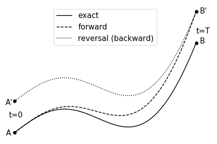
Figure 1: Schematic illustration of forward and time-reversal integrations for a dynamical system. The solid line represents the exact trajectory from $A$ at $t=0$ to $B$ at $t=T$. The dashed line is the numerical integration, which becomes $B^{\prime}$ at $t=T$. The difference between $B$ and $B^{\prime}$ indicates the chaos, but in practice, $B$ is usually unknown. The dotted line is the time-reversal integration starting from $B^{\prime}$ and ending at $A^{\prime}$. The difference between two initial conditions $A$ and $A^{\prime}$ is an indicator of chaos of the system for this specific initial condition.

The principle of the F-R integration approach can be briefly outlined as follows: A nonlinear transfer function, denoted as $f$, propagates through an $N$-dimensional phase space coordinate $\boldsymbol{z}=\left(x_{1},x_{2},\cdots,x_{N};p_{1},p_{2},\cdots,p_{D}\right)^{T}$ iteratively. In a finite-precision computation process, the iteration from the $(n-1)^{\text{th}}$ state $\boldsymbol{z}_{n-1}$ to the next state $\boldsymbol{z}_{n}$ reads as:

$$\boldsymbol{z}_{n}=f\left(\boldsymbol{z}_{n-1}\right)+\Delta\boldsymbol{z}_{n}.$$ (4)

where $\Delta\boldsymbol{z}_{n}=\left(\Delta x_{1},...,\Delta x_{N};\Delta p_{1},\dots,\Delta p_{N}\right)^{T}$ is the round-off error vector when performing the $n^{\text{th}}$ iteration. Similarly, the reversal integration can be written as,

$$\boldsymbol{z}_{n-1}^{\prime}=f^{-1}\left(\boldsymbol{z}_{n}^{\prime}\right)+\Delta\boldsymbol{z}_{n}^{\prime},$$ (5)

where, $f^{-1}$ is the inverse map, and primes (^′) denote the coordinates of the reversal so as to distinguish from the forward trajectory. The errors $\Delta\boldsymbol{z},\;\Delta\boldsymbol{z}^{\prime}$ are distributed uniformly and randomly within a range determined by the values of $\boldsymbol{z},\;\boldsymbol{z}^{\prime}$, and the number of bit of the computation unit [28].

When considering a case in which only one F-R iteration is computed, $\boldsymbol{z}_{0}\overset{f}{\rightarrow}\boldsymbol{z}_{1}\overset{f^{-1}}{\rightarrow}\boldsymbol{z}_{0}^{\prime}$. The difference between $\boldsymbol{z}_{0}$ and $\boldsymbol{z}_{0}^{\prime}$ can be estimated with local linear derivatives,

$$\boldsymbol{z}_{0}^{\prime}-\boldsymbol{z}_{0} =f^{-1}\left(f(\boldsymbol{z}_{0})+\Delta\boldsymbol{z}_{1}\right)+\Delta\boldsymbol{z}_{1}^{\prime}-\boldsymbol{z}_{0}$$

$$\approx\frac{\partial f^{-1}}{\partial\boldsymbol{z}}\biggr{\rvert}_{f(\boldsymbol{z}_{0})}\Delta\boldsymbol{z}_{1}+\Delta\boldsymbol{z}_{1}^{\prime}$$

$$=\left[\frac{\partial f}{\partial\boldsymbol{z}}\biggr{\rvert}_{\boldsymbol{z}_{0}}\right]^{-1}\Delta\boldsymbol{z}_{1}+\Delta\boldsymbol{z}_{1}^{\prime},$$ (6)

where the inverse Jacobian matrix of $f$ is evaluated at $\boldsymbol{z}_{0}$. For the sake of simplicity, the linearized matrix for 1-dimension $x$-$p$ is shown as,

$$\left[\frac{\partial f}{\partial\boldsymbol{z}}\biggr{\rvert}_{\boldsymbol{z}_{0}}\right]^{-1}=\left[\begin{array}[]{cc}\frac{\partial x_{1}}{\partial x_{0}}&\frac{\partial x_{1}}{\partial p_{0}}\\ \frac{\partial p_{1}}{\partial x_{0}}&\frac{\partial p_{1}}{\partial p_{0}}\end{array}\right]^{-1}.$$ (7)

Equation 2 indicates that the difference $|\boldsymbol{z}_{0}^{\prime}-\boldsymbol{z}_{0}|$ originates from random round-off errors, which are scaled by an inverse Jacobian matrix Eq. 7 on the passage of $\boldsymbol{z}_{0}$.

The difference, $\left|\boldsymbol{z}_{0}^{\prime}-\boldsymbol{z}_{0}\right|$, from one iteration can sometimes be impacted by random round-off noise, rather than the dynamical systems themselves as desired. On the other hand, if chaos is sufficiently weak, the difference is still invisible by just one-time scaling. Therefore, to overcome this difficulty, it may be necessary to implement multiple iterations, $\boldsymbol{z}_{0}\overset{f^{N}}{\rightarrow}\boldsymbol{z}_{N}\overset{f^{-N}}{\rightarrow}\boldsymbol{z}_{0}^{\prime}$, ($N\geq 2$). The difference can be estimated similarly as Eq. 2,

$$\left(\boldsymbol{z}_{0}^{\prime}-\boldsymbol{z}_{0}\right){}_{N} \approx\Delta\boldsymbol{z}_{1}^{\prime}+\sum_{n=2}^{N}\left(\prod_{j=0}^{n-2}\left[\frac{df}{d\boldsymbol{z}}\biggr{\rvert}_{\boldsymbol{z}=f^{j}\left(\boldsymbol{z}_{0}\right)}\right]^{-1}\right)\Delta\boldsymbol{z}^{\prime}_{n}$$

$$+\sum_{n=1}^{N}\left(\prod_{j=0}^{n-1}\left[\frac{df}{d\boldsymbol{z}}\biggr{\rvert}_{\boldsymbol{z}=f^{j}\left(\boldsymbol{z}_{0}\right)}\right]^{-1}\right)\Delta\boldsymbol{z}_{n}.$$ (8)

Here $f^{j}$ represents the value of the $j^{\text{th}}$-iterations of the map $f$ without round-off error. Equation 2 illustrates that round-off errors are accumulated during each iteration and are then scaled by local linear matrices along the trajectories in both directions. With sufficient iterations, the cumulative difference indicates the chaos of the trajectory.

It is worth noting that, even if a system has no chaos, the cumulative random error between forward integration and its corresponding reversal is directly proportional to the number of iterations executed [29]. If chaos is present, however, the error will grow exponentially.

In large scale modern accelerators, F-R integrations need to be evaluated magnet-by-magnet. A full cycle around an accelerator equates to one iteration as described above. The round-off errors $\Delta\boldsymbol{z}$ receive a contribution from each integration step. A short-term tracking simulation could generate an observable difference when 64 bit floats were used. To be specific, only one-turn F-R integrations are sufficient to optimize the DA of the NSLS-II storage ring. Usually these differences are observable but still at quite a small scale. Therefore, a base-ten logarithm is used to allow a large range to better represent them,

$$\Delta=\log_{10}|\boldsymbol{z}_{0}-\boldsymbol{z}_{0}^{\prime}|.$$ (9)

3 Hénon map

In this section, the F-R integration method is used to study a 1-dimensional Hénon map,

$$\left(\begin{array}[]{c}x\\ p\end{array}\right)_{n}=\left(\begin{array}[]{cc}\cos\mu&\sin\mu\\ -\sin\mu&\cos\mu\end{array}\right)\left(\begin{array}[]{c}x\\ p-x^{2}\end{array}\right)_{n-1}.$$ (10)

This discrete Hénon map represents a thin-lens sextupole kick followed by a linear phase space rotation at a phase advance $\mu$. Its reversal map can be expressed as an inverse rotation followed by an inverse thin-lens kick,

$$\left(\begin{array}[]{c}x_{t}\\ p_{t}\end{array}\right) =\left(\begin{array}[]{cc}\cos\mu&-\sin\mu\\ \sin\mu&\cos\mu\end{array}\right)\left(\begin{array}[]{c}x\\ p\end{array}\right)_{n},$$ (17)

$$\left(\begin{array}[]{c}x\\ p\end{array}\right)_{n-1} =\left(\begin{array}[]{c}x_{t}\\ p_{t}+x_{t}^{2}\end{array}\right),$$ (22)

where $x_{t},\;p_{t}$ are the intermediate variables.

The Hénon map’s linear phase advance is chosen as $\mu=0.205\times 2\pi$ in order to observe the $5^{\text{th}}$-order resonance line at certain amplitudes. The difference between initial conditions obtained from the F-R integration is illustrated in Fig. 2. When the F-R integrations are calculated with only 10-50 iterations (as shown in the top row), the area of the stable region is overestimated and the inside resonances are almost invisible. After 100 iterations, the resonance lines and stable islands become gradually visible. More iterations can provide much more detailed chaos information as illustrated in the two bottom subplots.

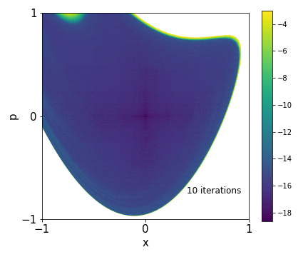
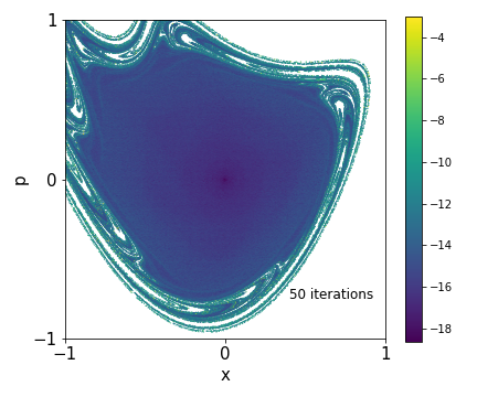
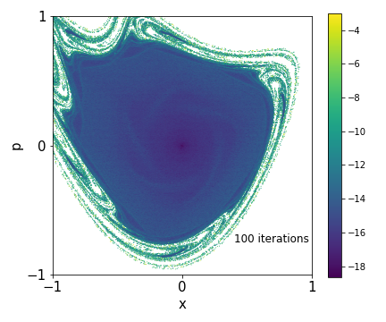
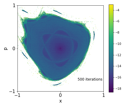
Figure 2: (Colored) Contour of the F-R integrations with different numbers of iterations for a Hénon map. The colormap are the difference of initial conditions as a function of the phase space coordinates $x$-$p$. The white area represents unbounded trajectories by manually setting a threshold of $|x|>10$. More iterations provide more detailed chaos information, but even with just a few dozen iterations, an early indicator of chaos can be determined.

4 Applications

In this section we demonstrate this method by optimizing the dynamic apertures for the National Synchrotron Light Source II (NSLS-II) [30] main storage ring and a test diffraction-limited light source ring.

4.1 NSLS-II storage ring

NSLS-II is a dedicated $3^{\text{rd}}$ generation medium energy (3 GeV) light source operated by Brookhaven National Laboratory. Its main storage ring’s lattice is a typical double-bend-achromat structure. Its linear optics for one cell is illustrated in Fig. 3. The whole ring is composed of 30 such cells. The natural chromaticities are corrected to $+2/+2$ at the transverse plane by the chromatic sextupoles. The optimization knobs are six families of harmonic sextupoles located at dispersion-free sections. The goal of optimization is to obtain a sufficient DA ($|x|>15\;\textrm{mm},|y|>5\;\textrm{mm}$) for the off-axis injection at the long straight section center where $\beta_{x}=20.5\;\textrm{m},\;\beta_{y}=3.4\;\textrm{m}$, and a $|\delta|>2.5\%$ momentum acceptance to ensure a 3 hour lifetime at a 500 mA beam current.

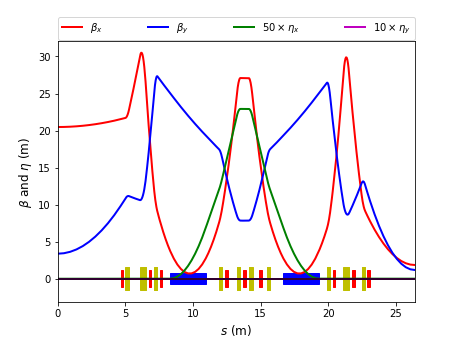
Figure 3: (Colored) The linear optics and magnet layout for one of the 30 cells of the NSLS-II storage ring. The red blocks represent sextupoles. The three located between two dipoles are used to correct the natural chromaticity. The remaining six are used here for DA optimization.

4.2 Optimization objectives and results

On the transverse $x$-$y$ plane at the injection point, multiple initial conditions are uniformly populated within a Region Of Interest (ROI). The ROI is chosen to cover the needed aperture. The virtual particle trajectories are simulated with a $4^{th}$ order kick-drift symplectic integrator [31] in which negative physical length elements are allowed. The symplectic integration is implemented with a python code, which has been independently benchmarked with another reliable tracking simulation code impactz [32]. After evolving some revolutionary periods (usually an integer number of turns), their reversal trajectories are computed by switching the sign of the coordinate $s$ and letting particles run back to $s=0$. Newly re-established initial conditions deviate from the original ones. A forward integration and its reversal make up a pair of trajectories for comparison. A larger difference between a pair of initial conditions indicate a stronger chaos. The goal of optimization then becomes minimizing the difference for all pairs of initial conditions within the ROI. It is not practical or necessary to minimize so many pairs of initial conditions simultaneously, therefore, the ROI is divided into several zones as shown in Fig. 4. For each zone, the difference of initial conditions are averaged over all F-R integrations pairs. Then the averaged values for all zones are used as the optimization objectives, which need to be minimized simultaneously to suppress the chaos inside the whole ROI. The optimization objective functions $g$ reads as

$$\bar{\Delta}_{i}=g_{i}(K_{2,j}),$$ (23)

where, $i,\;j$ are the indices of the ROI zones and the sextupoles respectively, $\bar{\Delta}_{i}$ is the average difference in the $i^{th}$ zone, and $K_{2,j}$ is the $j^{th}$ sextupole’s normalized gradient.

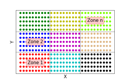
Figure 4: (Colored) Dividing the region of interest (ROI) into $n$ zones in the $x$-$y$ plane. In each zone, multiple initial conditions (represented with same-colored dots) are uniformly populated. The optimization objectives are the difference between the initial conditions of F-R integrations averaged over each zone.

Quantitatively, the difference in Eq. 9 and  23 for a pair of initial conditions in the normalized phase space can be computed as

$$\Delta=\log_{10}\sqrt{\Delta\bar{x}^{2}+\Delta\bar{p}_{x}^{2}+\Delta\bar{y}^{2}+\Delta\bar{p}_{y}^{2}},$$ (24)

where $\bar{x},\;\bar{p}_{x};\;\bar{y},\;\bar{p}_{y}$ are the difference of canonical coordinates normalized with Courant-Snyder parameters as follows [33],

$$\begin{bmatrix}\Delta\bar{u}\\ \Delta\bar{p}_{u}\end{bmatrix}=\begin{bmatrix}\frac{1}{\sqrt{\beta_{u}}}&0\\ \frac{\alpha_{u}}{\sqrt{\beta_{u}}}&\sqrt{\beta_{u}}\end{bmatrix}\begin{bmatrix}\Delta u\\ \Delta p_{u}\end{bmatrix}.$$ (25)

where $u=x,\;\text{or}\;y$, The normalization of Eq. 25 expresses the canonical coordinate pairs in the same units $m^{1/2}$ for arithmetic addition.

To obtain sufficient beam lifetime and DA simultaneously, one must optimize them simultaneously [34]. Direct optimization of beam lifetime is time-consuming. An alternative is to optimize different off-momentum DA. This was achieved by a $\delta$-slicing method as illustrated in Fig. 5. First, the desired energy acceptance range is determined based on the beam scattering lifetime calculation at a certain beam current. Then several sliced off-momentum DA are included into the optimization objectives. At each slice, the objective functions are evaluated in the same way as Fig. 4.

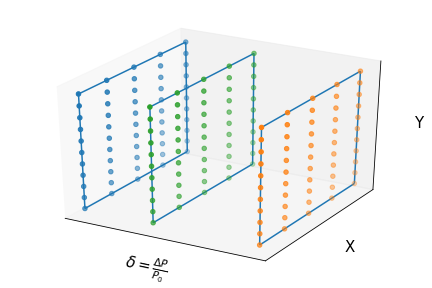
Figure 5: (Colored) Optimizing several fixed off-momentum DA simultaneously. By separating a 5-dimensional phase space ($x,p_{x};y,p_{y};\delta$) into several slices along the $\delta$-axis, DA for off-momentum particles can be optimized simultaneously.

Multiple zones within the ROI for different momentum slices need to be minimized simultaneously. The multi-objective genetic algorithm (MOGA) was used for this task. More turns of particle tracking simulation can indicate the chaos more accurately, but this requires more computation time. After manually checking the dependence of the chaos indicator against the number of turns, one-turn F-R integration (crossing 30 cells) was chosen to compute this early chaos indicator as illustrated in Fig. 6. Although the early indicator of chaos from F-R integration provides an optimistic approximation, it does rule out many of the less competitive candidates and narrows down the parameter search range quickly. By allowing a small-scale population, which includes the evolution of only 1,000 candidates over just 50 generations, the top candidates’ average fitness is seen to converge. It took about 6 hours to complete the optimization with 50 Intel^® Xeon^® 2.2-2.3 GHz CPU cores. Another reliable tracking code elegant [35] was then used to check the DA for all the candidates only inside the last generation. Among them, some of the elite candidates are selected for more extensive simulation studies to check their final performance.

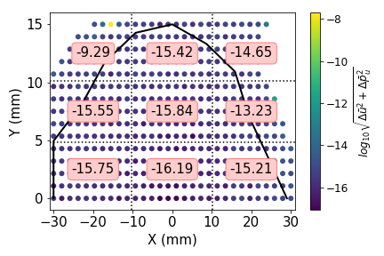
Figure 6: (Colored) The objective function evaluated in 9 zones for the $\delta=0$ slice. These were obtained for a specific set of sextupoles settings for the NSLS-II storage ring. Blank points represent lost particles ($|x,y|>1$ m) within 1 turn tracking. The maximum allowed number of lost particles is used as an optimization constraint. The black line is the dynamic aperture obtained by multi-turn (1,024) tracking simulation with the code elegant. The one-turn F-R integrations give a more optimistic result than the multi-turn tracking simulation. As an early indicator of chaos, however, it does provide a reasonable criteria for the optimizer.

The DA profiles for the top 100 candidates inside the last generation are illustrated in Fig. 7. Although the six sextupole families settings are very different, their DA satisfy the minimum requirement for top-off injection. This observation confirms that short-term F-R integration can indeed be used for DA optimization. Among these candidates, one from the elite cluster was selected to carry out a more detailed frequency map analysis (FMA) to verify its nonlinear dynamics performance. The FMA results are summarized later in Sect. 4.3.

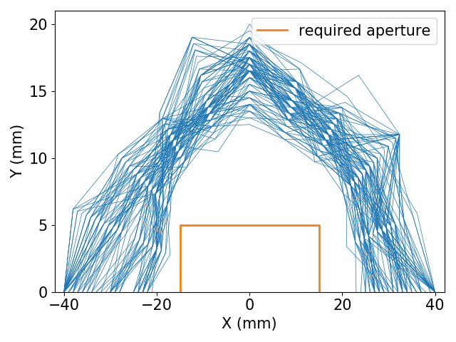
Figure 7: (Colored) DA of the top 100 candidates (measured with the area) from the $50^{th}$ generation of the evolved population obtained with the MOGA optimizer. The light yellow box is the required aperture for the off-axis top-off injection.

In the specific example of a dedicated light source machine (the NSLS-II storage ring), the longitudinal synchrotron oscillation has not been included. It is straightforward to include it if needed. It can be done by extending Eq. 24 to the 6-dimensional space when the betatron-synchrotron coupling resonances become critically important, e.g. in the case of collider rings.

4.3 Comparison with frequency map analysis

The frequency map analysis (FMA) is widely used to evaluate the performance of a nonlinear lattice [36, 37, 38, 39]. The FMA was also applied directly to optimizing the DA of a light source ring [40]. By comparing the tune diffusion rate determined by two pieces of turn-by-turn simulation or measurement data, the resonances of the lattice can be visualized. In our example, one elite solution was selected from the last generation of candidates to carry out a detailed FMA to characterize its nonlinear dynamics performance. In the meantime, a multi-turn (1,024 turns) F-R analysis was conducted for a comparison with the FMA results. The sextupole settings for the current NSLS-II lattice and the selected elite solution are listed in Tab. 1 for comparison.

Table 1: Comparison of two sextupoles settings

Sextupole	unit	$K_{2}$ (current)	$K_{2}$ (F-R)
SH1	$\textrm{m}^{-3}$	19.8329	19.8495
SH3	$\textrm{m}^{-3}$	-5.8551	-0.4017
SH4	$\textrm{m}^{-3}$	-15.8209	-22.0160
SL3	$\textrm{m}^{-3}$	-29.4609	-29.0057
SL2	$\textrm{m}^{-3}$	35.6779	27.9185
SL1	$\textrm{m}^{-3}$	-13.2716	-2.6051

Figure 8 illustrates the on-momentum DA in the transverse $x$-$y$ plane. Figure 9 shows the off-momentum acceptance in the $x$-$\delta$ plane. The FMA results yield more copious and fine patterns of the resonance than the FRI results. Even the accuracy of the NAFF can be theoretically proportional to $1/N^{4}$ ($N$ is the total number of the sampling data) with a Hanning window [41], it is still relatively slower compared to the exponential improvement of the reversal method. Therefore, a much less number of the FRI tracking is needed to drive the optimizer. In the previous example, only one-turn FRI has been used to speed up the convergence.

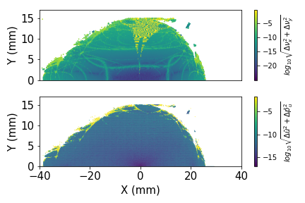
Figure 8: (Colored) Top: FMA on the $x$-$y$ plane for 1,024 turns of data (512 leading and 512 trailing turns) with the code elegant. Bottom: F-R analysis for 1,024 turns. Using the FMA, some unusual diffusion rate (as shown in yellow stripes near $x=0$) can be observed.

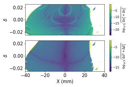
Figure 9: (Colored) Top: FMA on the $x$-$\delta$ plane for 1,024-turns of data (512 leading and 512 trailing turns) with the code elegant. Bottom: F-R analysis for 1,024 turns.

A control of higher order chromaticities and amplitude-dependent-tune-shifts to avoid destructive resonance-crossing is critical in DA optimization. This could be achieved by minimizing some specific nonlinear driving terms [42, 43]. For example, $C_{2200,0},C_{0022,0},C_{1111,0}$ are the first order amplitude-dependent-tune-shift coefficients; then $C_{1100,n},C_{0011,n},n\geq 2$ are the higher order chromaticity coefficients. These terms can be used as either objective functions or explicit constraints. In the F-R integration method, no explicit constraints are used to limit them. The final tracking simulation on the selected solution, however, shows that both the amplitude-dependent-tune-shifts (Fig. 10) and the higher order chromaticities (Fig. 11) are automatically and passively suppressed. The on-momentum and two off-momentum ($\pm 2.5\%$) DA, computed with the code elegant, are shown in Fig. 12.

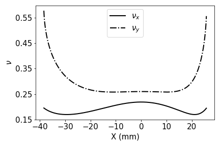
Figure 10: Tune shift with initial coordinate in the horizontal plane for the selected candidate. Although the vertical tune rises suddenly faster at larger horizontal amplitudes, the tune variations are within $\pm 0.03$ inside the range of $x\in[-15,15]\;\textrm{mm}$.

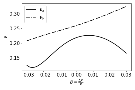
Figure 11: Tune variation with the momentum offset, i.e. chromaticity for the selected candidate. The linear chromaticities were tuned to +2 for both $x$ and $y$ planes.

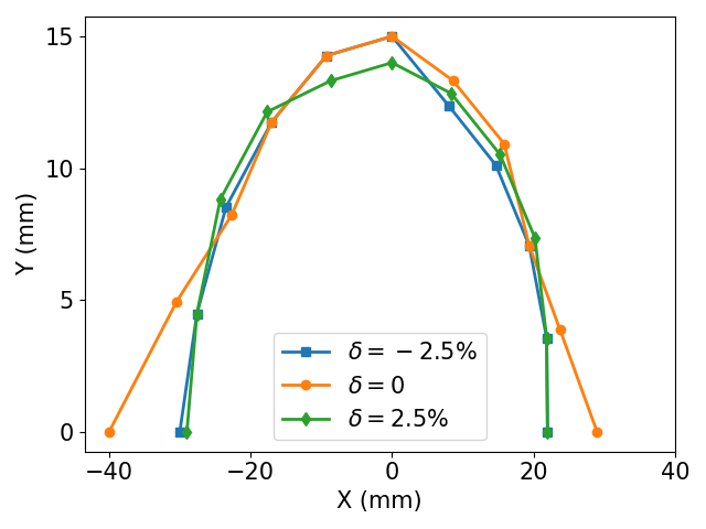
Figure 12: (colored) On- and two off-momentum ($\delta=\pm 2.5\%$) DAs for the selected candidate.

The optimization was implemented on an error-free model. Then the systematic and random magnetic field errors and the misalignments have been included to confirm the robustness of the solution. An online beam test on the NSLS-II storage ring was also carried out to confirm that the off-axis top-off injection efficiency is between 95-100%, which is comparable with our current operation lattice. The beam lifetime at a 400 mA beam current is longer than 5.5 hour, with a diffraction-limited vertical beam emittance of 8 pm. While the current operation lattice was observed having 4.5 hours in similar conditions.

4.4 MBA lattice for diffraction-limited light source

The F-R integration method has also been used to test on a multi-bend-achromat (MBA) structure, which could potentially be used as a diffraction-limited light source storage ring lattice in the future. The horizontal emittance of the test MBA lattice used was 78 pm at a beam energy of 2 GeV. The linear lattice is shown in Fig. 13, in which most sextupoles are chromatic sextupoles. The MOGA result showing the top 100 candidates’ apertures are illustrated in Fig. 14. The preliminary result confirms that the F-R integration could also be applied to a more complicated nonlinear lattice, and the approach itself should be general in optimizing other lattices.

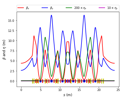
Figure 13: (Colored) Linear optics and magnet layout for one cell of a test MBA lattice.

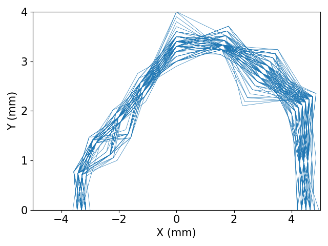
Figure 14: (Colored) On-momentum DA for the top 100 candidates for the test MBA lattice.

5 Summary

An indicator of chaos obtained with forward-reversal integration has been used for optimization of dynamic aperture of storage rings. The indicator, intrinsically but empirically associated with the Lyapunov exponent, gives an early indication of the chaos of beam motion in storage rings. Although the indicator cannot give the exact dynamic aperture profile with a short-term tracking simulation, a concrete correlation and large MOGA candidate pool yield some optimal lattice solutions. The NSLS-II storage ring and a test MBA lattice are used as examples to illustrate the application of this method.

The computation of the difference of F-R integrations has been implemented in the elegant [35] code since version 2019.4.0. Besides the F-R integration, the elegant code also provides another option for the users to compute the change in linear actions $J_{x,y}$ from two forward-only trackings, with a small difference in their initial conditions. By properly choosing small changes based on the machine precision, the signs and absolute values of initial conditions, and the round-off method in computer operation system, one should be able to get a similar result as the F-R integration. However, the needed implementation in this option is more complicated than the F-R integration. The fundamental principle of this method is to numerically characterize the sensitivity of a chaotic motion to its initial conditions by using round-off errors.

References

- [1] F. Zimmermann, Comparison of calculated with measured dynamic aperture, Conf. Proc. C940627 (1994) 327–331.
-
[2]
S. Habib, R. D. Ryne,
Symplectic
calculation of lyapunov exponents, Phys. Rev. Lett. 74 (1995) 70–73.
doi:10.1103/PhysRevLett.74.70.
URL https://link.aps.org/doi/10.1103/PhysRevLett.74.70 - [3] W. Scandale, Dynamic aperture, AIP Conf. Proc. 326 (1995) 52–97, [,52(1997)]. doi:10.1063/1.47306.
- [4] M. Giovannozzi, W. Scandale, E. Todesco, Inverse logarithm decay of long term dynamic aperture in hadron colliders, in: 17th IEEE Particle Accelerator Conference (PAC 97): Accelerator Science, Technology and Applications Vancouver, British Columbia, Canada, May 12-16, 1997, 1997.
- [5] M. Giovannozzi, W. Scandale, E. Todesco, Dynamic aperture extrapolation in presence of tune modulation, Phys. Rev. E57 (1998) 3432–3443. doi:10.1103/PhysRevE.57.3432.
-
[6]
G. Turchetti, F. Panichi,
Birkhoff
normal forms and stability indicators for betatronic motion, 2018, pp.
47–69.
URL https://www.worldscientific.com/doi/abs/10.1142/9789813279612_0004 - [7] F. Schmidt, Untersuchungen zur dynamischen akzeptanz von protonenbeschleunigern und ihre begrenzung durch chaotische bewegung, Tech. Rep. DESY HERA 88-02 (1988).
- [8] W. Fischer, An experimental study on the long-term stability of particle motion in hadron storage rings, Ph.D. thesis, Hamburg U., Hamburg (2005).
- [9] F. Schmidt, F. Willeke, F. Zimmermann, Comparison of methods to determine long-term stability in proton storage rings 35.
-
[10]
A. Wolf, J. B. Swift, H. L. Swinney, J. A. Vastano,
Determining
lyapunov exponents from a time series, Physica D: Nonlinear Phenomena 16 (3)
(1985) 285 – 317.
doi:https://doi.org/10.1016/0167-2789(85)90011-9.
URL http://www.sciencedirect.com/science/article/pii/0167278985900119 - [11] F. T. Cole, Oh Camelot!: A memoir of the MURA years.
- [12] R. H. Miller, Irreversibility in Small Stellar Dynamical Systems., Astrophysical Journal 140 (1964) 250. doi:10.1086/147911.
- [13] R. Genesio, A. Vicino, New techniques for constructing asymptotic stability regions for nonlinear systems, IEEE transactions on circuits and systems 31 (6) (1984) 574–581.
- [14] H.-D. Chiang, M. W. Hirsch, F. F. Wu, Stability regions of nonlinear autonomous dynamical systems, IEEE Transactions on Automatic Control 33 (1) (1988) 16–27.
- [15] M. Loccufier, E. Noldus, A new trajectory reversing method for estimating stability regions of autonomous nonlinear systems, Nonlinear dynamics 21 (3) (2000) 265–288.
- [16] H.-K. Lee, K.-W. Han, Analysis of nonlinear reactor systems by forward and backward integration methods, IEEE Transactions on Nuclear Science 47 (6) (2000) 2693–2698.
- [17] L. Jaulin, I. Braems, M. Kieffer, E. Walter, Nonlinear state estimation using forward-backward propagation of intervals in an algorithm, in: Scientific computing, validated numerics, interval methods, Springer, 2001, pp. 191–201.
- [18] K. Hwang, C. Mitchell, R. Ryne, Chaos Indicators for Studying Dynamic Aperture in the IOTA Ring with Protons, in: Proceedings, 10th International Particle Accelerator Conference (IPAC2019): Melbourne, Australia, May 19-24, 2019, 2019, p. WEPTS078. doi:10.18429/JACoW-IPAC2019-WEPTS078.
- [19] K. Deb, Multi-Objective Optimization Using Evolutionary Algorithms, Wiley, 2001.
-
[20]
L. Yang, D. Robin, F. Sannibale, C. Steier, W. Wan,
Global
optimization of an accelerator lattice using multiobjective genetic
algorithms, Nuclear Instruments and Methods in Physics Research Section A:
Accelerators, Spectrometers, Detectors and Associated Equipment 609 (1)
(2009) 50 – 57.
doi:http://dx.doi.org/10.1016/j.nima.2009.08.027.
URL http://www.sciencedirect.com/science/article/pii/S0168900209016040 -
[21]
L. Yang, Y. Li, W. Guo, S. Krinsky,
Multiobjective
optimization of dynamic aperture, Phys. Rev. ST Accel. Beams 14 (2011)
054001.
doi:10.1103/PhysRevSTAB.14.054001.
URL https://link.aps.org/doi/10.1103/PhysRevSTAB.14.054001 - [22] Y. Li, L. Yang, Multi-objective dynamic aperture optimization for storage rings, Int. J. Mod. Phys. A31 (33) (2016) 1644019. doi:10.1142/S0217751X1644019X,10.1142/9789813220089_0019.
-
[23]
Y. Li, W. Cheng, L. H. Yu, R. Rainer,
Genetic
algorithm enhanced by machine learning in dynamic aperture optimization,
Phys. Rev. Accel. Beams 21 (2018) 054601.
doi:10.1103/PhysRevAccelBeams.21.054601.
URL https://link.aps.org/doi/10.1103/PhysRevAccelBeams.21.054601 -
[24]
J. Wan, P. Chu, Y. Jiao, Y. Li,
Improvement
of machine learning enhanced genetic algorithm for nonlinear beam dynamics
optimization, Nuclear Instruments and Methods in Physics Research Section A:
Accelerators, Spectrometers, Detectors and Associated Equipment 946 (2019)
162683.
doi:https://doi.org/10.1016/j.nima.2019.162683.
URL http://www.sciencedirect.com/science/article/pii/S0168900219311611 -
[25]
A. Liu, A. Bross, D. Neuffer,
Optimization
of the magnetic horn for the nuSTORM non-conventional neutrino beam using
the genetic algorithm, Nuclear Instruments and Methods in Physics Research
Section A: Accelerators, Spectrometers, Detectors and Associated Equipment
794 (2015) 200 – 205.
doi:https://doi.org/10.1016/j.nima.2015.05.035.
URL http://www.sciencedirect.com/science/article/pii/S0168900215006750 -
[26]
A. Liu, A. Bross, D. Neuffer,
A FODO
racetrack ring for nuSTORM: design and optimization, Journal of
Instrumentation 12 (07) (2017) P07018–P07018.
doi:10.1088/1748-0221/12/07/p07018.
URL https://doi.org/10.1088%2F1748-0221%2F12%2F07%2Fp07018 - [27] G. Ripken, Nonlinear canonical equations of coupled synchrobetatron motion and their solution within the framework of a nonlinear six-dimensional (symplectic) tracking program for ultrarelativistic protons, DESY-85-084.
- [28] I. . Committee, Ieee standard for floating-point arithmetic, Tech. Rep. 754-2019, Microprocessor Standards Committee of the IEEE Computer Society, New York, NY (2019). doi:10.1109/IEEESTD.2008.4610935.
- [29] J. Laslett, Round-Off Errors From Fixed-Point Linear Algebraic Transformations Computer by IBM-704 Program 117.
- [30] BNL, https://www.bnl.gov/nsls2/project/PDR/.
- [31] H. Yoshida, Construction of higher order symplectic integrators, Phys. Lett. A150 (1990) 262–268. doi:10.1016/0375-9601(90)90092-3.
-
[32]
J. Qiang, R. D. Ryne, S. Habib, V. Decyk,
An
object-oriented parallel particle-in-cell code for beam dynamics simulation
in linear accelerators, Journal of Computational Physics 163 (2) (2000) 434
– 451.
doi:https://doi.org/10.1006/jcph.2000.6570.
URL http://www.sciencedirect.com/science/article/pii/S0021999100965707 -
[33]
E. Courant, H. Snyder,
Theory
of the alternating-gradient synchrotron, Annals of Physics 3 (1) (1958) 1 –
48.
doi:https://doi.org/10.1016/0003-4916(58)90012-5.
URL http://www.sciencedirect.com/science/article/pii/0003491658900125 - [34] M. Borland, L. Emery, V. Sajaev, A. Xiao, Multi-objective Optimization of a Lattice for Potential Upgrade of the Advanced Photon Source, Conf.Proc. C110328 (2011) 2354–2356.
-
[35]
M. Borland,
elegant:
A Flexible SDDS-Compliant Code for Accelerator Simulation, in: 6th
International Computational Accelerator Physics Conference (ICAP 2000)
Darmstadt, Germany, September 11-14, 2000, 2000.
doi:10.2172/761286.
URL https://www.aps.anl.gov/files/APS-sync/lsnotes/files/APS_1418218.pdf - [36] D. Robin, C. Steier, J. Laskar, L. Nadolski, Global Dynamics of the Advanced Light Source Revealed through Experimental Frequency Map Analysis, Phys. Rev. Lett. 85 (2000) 558–561. doi:10.1103/PhysRevLett.85.558.
- [37] J. Laskar, Frequency Map Analysis and Particle Accelerators, in: 20th Particle Accelerator Conference (PAC 03), 2003, p. 378.
-
[38]
Y. Papaphilippou, Detecting chaos in
particle accelerators through the frequency map analysis method, Chaos: An
Interdisciplinary Journal of Nonlinear Science 24 (2) (2014) 024412.
arXiv:https://doi.org/10.1063/1.4884495, doi:10.1063/1.4884495.
URL https://doi.org/10.1063/1.4884495 -
[39]
E. Todesco, R. Bartolini, A. Faus-Golfe, M. Giovannozzi, W. Scandale,
Early
indicators of long term stability in hadron colliders, in: Particle
accelerator. Proceedings, 5th European Conference, EPAC 96, Sitges, Spain,
June 10-14, 1996. Vol. 1-3, 1996, pp. 313–315.
URL http://accelconf.web.cern.ch/AccelConf/e96/PAPERS/ORALS/TUO01A.PDF - [40] C. Steier, W. Wan, Quantitative lattice optimization using frequency map analysis, Proc. of IPAC (2010) 4746–4748.
- [41] J. Laskar, Introduction to Frequency Map Analysis. In: Simó C. (eds) Hamiltonian Systems with Three or More Degrees of Freedom. NATO ASI Series (Series C: Mathematical and Physical Sciences)”, Vol. 533, Springer, Dordrecht, 1999, pp. 134–150.
-
[42]
A. J. Dragt, Lie
methods for nonlinear dynamics with applications to accelerator physics,
Unpublished, 2011.
URL http://www.physics.umd.edu/dsat/dsatliemethods.html - [43] A. Chao, Lecture notes on topics in accelerator physics, Unpublished, 2002.