Ultra slow electron holes in collisionless plasmas: stability at high ion temperature

Abstract

Numerical simulations recover ultra slow electron holes (EH) of electron-acoustic genre propagating stably well below the ion acoustic speed where the ion response disallows any known pure electron perturbation. The reason of stability of EH at high ion temperature ($T_{i}>T_{e}$) is traced to the loss of neutralizing cold ion response. In a background of cold ions, $\theta=T_{e}/T_{i}\gg 1$, they have an ion compression that accelerates to jump over a forbidden velocity gap and settle on the high velocity tail of the electron distribution $f_{e}$, confirming to a recently identified limit of the nonlinear dispersion relation. For $\theta=T_{e}/T_{i}\leq 1$, however, the warm ions begin to supplement the electron response transforming the ion compression to decompression at the hole location and triggering multiplicity of the scales in trapped electron population which prompts an immediate generalization of the basic EH theory.

I Introduction

The collective excitations in collisional plasmas are well represented by discrete linear waves below the amplitudes where the convective nonlinearity of fluid formulation begins to assume significance. In hot collisionless plasmas, however, the earliest (often vanishing) threshold to nonlinear behavior is introduced by the kinetic effects such that the waves very fast achieve coherency at unusually low amplitudes. The first accessible class of nonlinear collective excitations in hot plasmas therefore, in practice and in most numerical simulations, is that of the nonlinear particle trapping equilibria, such as the non-isothermal ion acoustic solitary waves, solitary and cnoidal electron and ion holes or various forms of double layers Saeki79 ; S79 ; Schamel (1972); S86 ; Krall and Trivelpiece (1986); Bernstein et al. (1957); Dupree (1983). These nonlinear modifications often render stability to rather exotic excitations in the plasma, for example, electron acoustic perturbation slower than ion acoustic speeds Johnston et al. (2009); Lesur et al. (2014); Petkaki et al. (2006); Mandal and Sharma (2016a) and electron holes structures in the circular particle beam, or synchrotron, experiments S97 ; BWLS04 ; LS05 .

The simplest nonlinear analytic approach to the experimentally and numerically observable class of excitations Mandal and Sharma (2014); Osmane et al. (2017); Eliasson and Shukla (2006); Saeki and Genma (1998); Pickett et al. (2004); Osborne (1994); Gurevich (1968); III et al. (2010) works by invoking a fixed ionic background and a thermal Maxwellian approximation for equilibrium electron distribution in the Vlasov analysis, for example in all well known linear landau; vancampan and nonlinear Schamel (2012) approaches. For the trapped electrons, however, a variety of Ans$\ddot{a}$tze is in principle possible but using a, thermalized (single parameter), distribution of trapped particles produces the simplest class of nonlinear solutions. Additionally, as long as the equilibrium distributions are thermalized and identical to those used for obtaining linear modes, the nonlinear solutions can still be identified as corresponding to the well known linear modes, however having noticeable (nonlinear) modification by trapped particles. For an easy reference, this limit of nonlinear Vlasov treatment is termed here as a Special Limit of Correspondence (SLC) of the general nonlinear Vlasov framework since the computer simulations of structures in collisionless plasmas are best interpreted by an approach in SLC, given the unavoidable numerical thermalization effects in them. We, for example, apply the one developed extensively by Schamel and co-authors Schamel (2012) which introduces amplitude dependence in the dispersion and removes much of discreteness of the linear wave solution space.

It was recently discovered Mandal et al. (2018), that the discreteness of the linear modes (distinct roots of linear dispersion function) also exists in the nonlinear solutions space (as corresponding band gaps) which was originally understood to be a continuum Schamel (2012) solution space. These band gaps, or forbidden velocity ranges, were identified to be allowed also by the hole theory after the simulations in Mandal et al. (2018) could achieve no stably propagating EH structures in particular velocity ranges. In more specific terms, the nonlinear EH structures were noted as unstable (i.e., not propagating coherently but accelerating) below a critical velocity value which almost ruled out existence of any electron holes slower than nearly the ion acoustic speed, explaining several past observations of accelerating holes in the simulations Zhou and Hutchinson (2016); Eliasson and Shukla (2004); Schamel et al. (2017). By applying the special correspondence, of the nonlinearly obtained limiting velocity value with the ion acoustic phase velocity in the linear theory, it appeared that the acoustic structures would not propagate below the ion acoustic speed in a typical plasmas where $T_{e}$ is sufficiently larger than $T_{i}$, essentially because of possibility of neutralizing ion response below this velocity (slow enough time scale). In this paper we however present a set of simulations showing that ultra slow electron holes regain their stability at large enough ion temperature which exceeds electron temperature. The associated nonlinear analytics shows that the band gap is a dynamical one and may indeed be buried with the changing ion temperature, showing no minimum cutoff velocity (e.g., the ion acoustic speed) for structures with no ion trapping.

With no significant contribution of resonant ions and a decompressed electron density, the observed ultra slow EH correspond to the electron-acoustic structures. They however have an unusual ion density profile which is also decompressed, in contrast to the ion compression in their usual velocity regime. In the conclusion of this paper we finally highlight an important issue that the theoretical recovery of these slow electron hole structure under the basic EH theory may be possible only by a further extension of the theory. Although such an extension and greater details of this analytic aspect is addressed in a dedicated forthcoming article MSS19 , the idea mainly pertain to phase-space topology of the trapped electron density of the observed ultra-slow stable electron hole structures summarized in following statements. While the observed slow EH are recovered to have a dip-like trapped electron density, the lowest order electron hole theory prescribes them to have exclusively a humped structure. A modification of the lowest order electron hole theory is however possible by appropriate higher order corrections, allowing it to yield a dip-like trapped electron density structure, as recovered numerically for these ultra slow structures, without causing any characteristic change in the associated pseudo-potential structure.

This paper is organized as follows. We present the results of our high resolution Vlasov simulations in Sec. II. The analytical model following the SLC of the Vlasov formulation is discussed and used to describe the results in Sec. III. The discussion of the physics of the observation and requirement of appropriate extension of the EH theory is highlighted in Sec IV and the summary and conclusions are presented in Sec. V.

II Simulation results

We performed Vlasov simulations using the Flux-Balance Fijalkow (1999); Mandal and Sharma (2016b) technique for both electrons and ions in the $x$-$v$ space with 8192 $\times$ 16384 dual mesh grid. A well localized initial perturbation is used in the electron distribution function with the analytic form of perturbation,

$$f_{1}(x,v)=-\epsilon~{}{\rm sech}\left[\frac{v-v_{1}}{L_{1}}\right]{\rm sech}^{4}[k(x-x_{1})]$$ (1)

where $\epsilon$ is the amplitude of the perturbation, $L_{1}$ is the width of the perturbation in the velocity dimension and $k^{-1}$ is its spatial width.

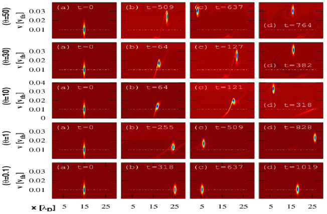
Figure 1: Evolution of the electron phase-space perturbation in all the five cases. In case-5 ($\theta=0.1$) the electron hole is not accelerated from its initial perturbation location. In all other cases they accelerate but their evolution time is different. The cases with lower ion temperature (high $\theta$) take more time to construct a valid electron hole solution from the initial perturbation. (The color scale is used for the value of electron distribution function, increasing linearly from blue to red.)

The background equilibrium velocity distribution of the electrons is a shifted Maxwellian and that of the ions an unshifted Maxwellian, given in normalized quantities by

$$f_{0e}(v) = \frac{1}{\sqrt{2\pi}}\exp\left[-\frac{(v-v_{D})^{2}}{2}\right]$$ (2)

$$f_{0i}(u) = \frac{F_{0}}{\sqrt{2\pi}}\exp\left[-\frac{u^{2}}{2}\right]$$ (3)

where $v$ is normalized by $v_{the}=\sqrt{\frac{T_{e}}{m_{e}}}$ and $u$ by $v_{thi}=\sqrt{\frac{T_{i}}{m_{i}}}$, respectively. Therefore $u=v\sqrt{\theta/\delta}$, where $\theta=T_{e}/T_{i}$ and $\delta=m_{e}/m_{i}$. Subscripts $j=e,i$ correspond to electron and ion species, respectively. The factor $F_{0}$ is ratio of total ion and electron content in the simulation region ($\int\int f_{e}dxdv/\int\int f_{i}dxdv$), ensuring that the same number of ions and electrons are present in the simulation box. In the simulation we use the Debye length $\lambda_{D}$, electron plasma frequency $\omega_{pe}$ and electron thermal velocity $v_{the}$ as normalizations for length, time and electron velocities, respectively. According to linear theory of plasma, the critical linear threshold ($v^{*}_{D}$), required minimum drift value $v_{D}$ for a current driven ion acoustic instability, becomes $v^{*}_{D}=0.053$ for $\theta=T_{e}/T_{i}=10$ and $\delta=m_{e}/m_{i}=1/1836$. For all the cases our choice of the drift velocity is $v_{D}=0.01$ which is well below the linear threshold for those temperature ratios Krall and Trivelpiece (1986); Landau (1944).

We first present the evolution of the total electron distribution $f_{e}=f_{0e}+f_{1}$ in cases 1-5 having $\theta=50$, $30,10,1$ and $0.1$, as plotted in Fig.1, respectively, showing result of varying ion response in them. Considering the temperature dependency, the ion acoustic wave phase velocity in one dimension for these five cases are $C_{s}=0.033,0.036,0.045,0.093$, and $0.24v_{the}$, where $C_{s}=(\sqrt{\delta}+\gamma\sqrt{\delta/\theta})~{}v_{the}$ with $\gamma=3$. Therefore in all the cases the initial electron velocity perturbation location $v_{1}=0.01~{}v_{the}$ is well below the corresponding $C_{s}$ and also the drift velocity $v_{D}$ is well below the corresponding critical linear thresholds $v_{D}^{*}$. Moreover, in the last case the ion temperature is higher than the electron temperature. A nonlinear plasma response to the applied perturbation, in the form of amplitude dependent propagating coherent structures, is nevertheless seen in all the cases where the perturbation of the form (1) is placed at $x=15$ in the simulation box having the length $L=30$. The velocity perturbation location in all cases is $v_{1}=0.01$ with phase-space widths of the perturbation $L_{1}=0.01$ along the velocity dimension and $k^{-1}=10$ along the spatial dimension $x$. The strength of the perturbation is small: $\epsilon=0.02$. As witnessed in our earlier simulations, being placed at such small velocity the initial perturbation with $\theta>1$ is unstable and experiences an acceleration. For the last case with $\theta=0.1$, however, the time evolution of the contours of electron distribution function $f_{e}(x,v)$ in phase-space, presented in last row (from top) of Fig. 1, shows that the perturbation is largely intact and, after a marginal readjustment of its $x$-$v$ space widths, continues its propagation with nearly the original velocity, $0.01v_{the}$.

Considering insignificant contribution of resonant ions (a very narrow velocity range of ion trapping region, as compared to trapped electrons), the stability of electron holes for small $\theta$ is once again understood to be detrmined by collective shielding effects rather than resonant ion reflection Dupree (1983). In qualitative sense Mandal et al. (2018) it can be described as follows. In a stable hole, the flux of the cold ion density expelled by the positive potential of the perturbation balances the flux of ions pushed in by the relative excess of hot electrons surrounding the hole. Thus the stability is achieved at faster velocities because of smaller outflowing ion flux due to smaller exposure of background ions to the hole electric field Mandal et al. (2018). The stability at smaller velocity therefore presents an interesting case and indicates a new mechanism underlying the stable holes to overcome destabilizing cold ion response that, in the usual case of colder ions, necessitates a minimum velocity for the stability. The slow holes observed in our simulation are found to achieve this stability by marginalizing the cold ion response in the limit $\theta\ll 1$. We observe that the stability is achieved critically when the single (fully untrapped) ion population stops supplementing the response of cold electrons and instead begins to supplement the response of streaming Boltzmann electrons. This means the warm ions rather rarefact at the hole location in full accordance with the Boltzmann-like response of positive ions to a positive potential. This behavior of ion density is clearly visible in the ion density profiles shown in Fig. 2(a) and (b) for large and small values of $\theta$, respectiely.

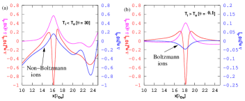
Figure 2: Electron density, ion density and potential prfiles for (a) $\theta$=30 and (b) $\theta$=0.1.

In the next section we examine this aspect more quantitatively and explain that these solutions are a special class of Cnoidal Electron Holes representing the nonlinear solutions of the Vlasov equation.

III Analytical Vlasov model, gaps of existence and quasi-particle interpretation

The existence regimes of Cnoidal Electron Holes (CEHs) and their dependence on the ion temperature are now evaluated in more quantitative terms using the non-perturbative nonlinear dispersion formulation of Schamel (see e.g. Schamel (2012) and references therein). Note that the description below is limited to finding the thresholds that bound the parameter regime in which the formal solutions of Vlasov equation, prescribed in Schamel (2012), represnt an undamped propagation. A solution outside these thresholds does not satisfy nonlinear dispersin relation and therefore must undergo a transient, or phasemix, i.e. an evolution which is not covered by a nonlinear dispersion formulation that aimes to identify only the coherently propagating solutions. A more detail description of the analytical model used here is given in Appendix-A. The phase velocity of a settled vortex structure in electron phase space is determined by the nonlinear dispersion relation (NDR) Eq. (12),

$$k_{0}^{2} - \frac{1}{2}Z_{r}^{{}^{\prime}}\left(\tilde{v}_{D}/\sqrt{2}\right)-\frac{\theta}{2}Z_{r}^{{}^{\prime}}\left(u_{0}/\sqrt{2}\right)=B,$$ (4)

where, $Z_{r}(x)$ is the real part of the plasma dispersion function. Depending on different values of $k_{0}$ and $B$ one gets different type of solutions, like solitary solution and cnoidal solutions. The right hand side of the equation presents the contribution of free electrons and ions and the left hand side presents the trapped particle contribution. Since in our case $v_{D}=0.01$, we can consider $-\frac{1}{2}Z_{r}^{{}^{\prime}}\left(\tilde{v}_{D}/\sqrt{2}\right)\sim 1$. For a solitary electron hole $k_{0}^{2}=0$, and the NDR Eq. (4) can be written as,

$$-\frac{1}{2}Z_{r}^{{}^{\prime}}\left(u_{0}/\sqrt{2}\right)=\frac{1}{\theta}(B-1)=:D.$$ (5)

Therefore, for our conditions of no ion trapping the phase velocity of the solutions are controlled by the ion temperature $\theta$ and electron trapping parameter $B(\beta,\psi)$.

A solution of Eq. (5) together with $B>0$ decides quantitatively about the existence of solutions. The solubility demands, $-0.285\leq D\leq 1$, as Fig. 3 shows, in which $-\frac{1}{2}Z^{\prime}_{r}(x)$ is plotted as a function of $x$. For $D\geq 0$ (or $B\geq 1$) one has one solution, and for $D<0$ (or $B<1$) one has two solutions.

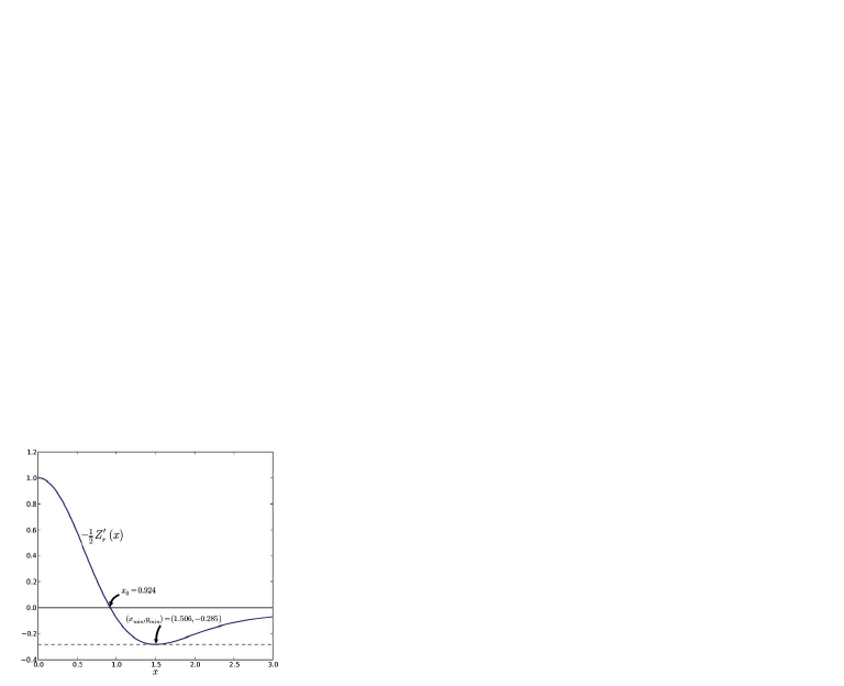
Figure 3: Plot of $-\frac{1}{2}Z^{\prime}_{r}(x)$ with $x$.

There are accordingly three velocity regimes:

$${\rm(i)}~{}~{}0.0 \leq u_{0}\leq 1.307~{}(=0.924\sqrt{2}),\qquad 1\leq B\leq 1+\theta$$

$${\rm(ii)}~{}1.307 < u_{0}\leq 2.12~{}(=1.5\sqrt{2}),\quad 1-0.285~{}\theta\leq B<1$$

$${\rm(iii)}~{}2.12 < u_{0}<\infty,\qquad\qquad\qquad 1-0.285~{}\theta\leq B<1.$$

The first two belong to the Slow Ion Acoustic branch (SIA), the third one to the ordinary Ion Acoustic branch (IA). In the second column the necessary conditions for $B$ are presented for given $\theta$, which are subject to $B>0$. This means that for the doublet of solutions, (ii), (iii), which satisfy the same constraints, ($-0.285\leq D<0$), there is a division line for $\theta$ given by $\theta^{*}:=\frac{1}{0.285}=3.51$. For $\bf{cold}$ ions, $\theta>\theta^{*}$, any $B$ in $0<B<1$ is admitted, whereas for $\bf{hot}$ ions, $\theta<\theta^{*}$, $B$ must satisfy $1-0.285~{}\theta\leq B<1$. In terms of $B$ we have therefore the following situation, for slow regime of SIA given by (i) $1\leq B\leq 1+\theta$ there is no other choice for a solution. But for $1-0.285\theta\leq B<1$, the plasma has two choices for establishing a solution, $u_{0}$ lies either on the faster part of the SIA branch (ii) or on the still faster velocity IA branch, regime (iii), with a gap in between.

Table 1: $v_{1}$, $u_{1}$, $v_{0}$, $u_{0}$, $B$ and velocity regime

$\theta$	$v_{1}$	$u_{1}=\sqrt{\frac{m_{i}\theta}{m_{e}}}v_{1}$	$v_{0}$	$u_{0}=\sqrt{\frac{m_{i}\theta}{m_{e}}}v_{0}$	$B$	v-regime
0.1	0.01	0.136	0.01	0.136	1.1	(i)
1	0.01	0.429	0.023	0.986	1.32	(i)
10	0.01	1.355	0.035	4.743	0.47	(ii) $\rightarrow$ (iii)

Tab: 1 presents the initial perturbation velocity $v_{1}$ (in electron frame), $u_{1}$ (in ion frame), final velocity at settled state $v_{0}$ (in electron frame), $u_{0}$ (in ion frame), $B$ values (from Eq. 5) and the velocity regime for these three cases $\theta=0.1,1$ and $10$. We define the case $\theta=50,30$ is identical with case $\theta=10$, because in all the three cases unstable electron holes saturate to same final velocity $v_{0}=0.035v_{the}$. Initially the perturbation is hence located for $\theta=(0.1,1)$ in (i) and for $\theta=10$ in (ii). Therefore, in the cases-4 and 5 with $\theta=1$ and $0.1$ the SEH will stay in the same velocity regime (i), and for the case-3 with $\theta=10$ there is a possibility of transition of solution from the velocity regime (ii) to (iii). Since ion acoustic velocity in the ion frame is given by $c_{s}:=\sqrt{\theta}$ we get the triplet $c_{s}=(0.32,1,3.16)$ and for the associated Mach numbers $M:=\frac{u_{0}}{c_{s}}$ the triplet (0.43, 1, 1.5). The SEH structure hence travels subsonically for hot and supersonically for cold ions, whereas it moves sonically for moderate ion temperatures. $\theta\approx 1$. This furthermore implies from Eq. (5) $B:(1.1,1.32,0.47)$ or $D:(0.95,0.32,-0.053)$. Whereas for $\theta=(0.1,1)$ the SEH remains in (i), i.e. in the ultra slow ion acoustic regime, for $\theta=10$ (and 30,50) the SEH makes a transition from (ii) to (iii), i.e. it accelerates and jumps from (ii) to (iii) crossing the gap of no solution (“forbidden region”) to settle in the supersonic regime.

The reason for an additional velocity gain by the solutions in some cases, even after achieving the valid set of parameters to qualify as solution of the nonlinear Vlasov equation, is that the SEH prefers to settle in a region of $\bf{negative}$ free energy GS02 . This enables the plasma, by approaching such lower energy state, to gain (harvest) energy which during the evolution is deposited for example as heat and/or in other fluctuations or excitations. This lower energy state is hence attractive and thus preferred by the plasma, which explains the additional acceleration observed for large $\theta$ even when the solutions are allowed by the NDR Mandal et al. (2018).

With respect to the pure kinetic effects of ions reflection as treated by Dupree Dupree (1983) not significantly visible in present cases Mandal et al. (2018), the simulations highlight the dominant role of streaming ion populaion in comparison to the reflected ion population duly accounted for in the present simulations. Note that the width, along the velocity dimension, of the ion trapping region is smaller by a factor $\sqrt{\theta/\delta}$ in comparison to that of electros because of higher kinetic energy of ions at similar velocities. In other words, a small amplitude structure would not trap/reflect as large fraction of ions density as that of electrons. Although this small reflected ion population effectively represnts a trapped ion population in our periodic setup, it does not maintain its identity, distinct form the streaming population, over its longer transit between two consequitive reflections (more so in the limit $L\rightarrow\infty)$. This justifies neglecting the ion trapping term $b(\alpha,u_{0})$, as in the NDR Eq. (12), since reftected/trapped ions may not effectively maintain an $\alpha$ value different from the unity. Moreover, for present EH having small $\psi<<T_{e}$ the net momentum transfered, because of finite $\partial f_{i}/\partial v$, by the imbalanced populations of reflected ions to the hole, as considered by Dupree Dupree (1983), is negligible given the narrow width of ion trapping region along the velocity dimension, as discussed above. Therefore, the response of streaming ions remains the most dominant factor in determining the observed stability of the hole solutions, as considered in the present analysis.

We close this theoretical part with a few experimentally relevant remarks on spontaneous acceleration of holes. A similar sudden acceleration of holes (in this case of a periodic train of ion holes) has been seen in the experiments of FKPS01 . Density fluctuation measurements in a double plasma device show an apparently spontaneous transition of these periodic structures from slow ion acoustic to ion acoustic velocity regime. In this experiment gradual scattering of the trapped ion population by elastic collisions with neutrals was made responsible for this transition. The outcome of our paper, however, suggests a second possibility as an alternative explanation, namely the tendency of the plasma to achieve a lower energy status during the evolution, a process which will be the more probable the more dilute the plasma is.

IV Missing hump and extension of the basic EH theory

We now indicate an advanced feature of the Electron hole solutions identified in the present simulation output which might require extension of the basic EH theory to include a newer parameter to accommodate multiplicity of scales in trapped electron density.

Note that the solution in Sec. III are discussed under the approximation $k_{0}^{2}=0$, appropriate for a solitary EH with depressed trapped electron electron density. However, when we examine the numerically recovered values of quantity $k$ carefully, the basic EH theory for these numerical $k$ values prescribes that for small $\theta$ solution the electron density must feature a hump like profile. The plasma, however, avoids this less stable state by transiting to a multiple-scale state of the trapped density where the central phase-space density of the trapped electrons still features a sharp dip, surrounded by a relatively flatter density profiles. Quantitatively, this situation is resolvable only by introducing more sophistication in the hole theory, which is a topic addressed in a forthcoming article dedicated to this issue and such a generalizing modification of the EH theory MSS19 .

V Summary and Conclusions

In summary, we have proved numerically and theoretically the stable existence of hole solutions in subcritical plasmas occurring at very low ion temperature values. This outcome is striking as it manifests the electron trapping nonlinearity as the ruling agent in this evolutionary process standing outside the realm of linear wave theory. We could show that the potential $\phi(x)$ is essentially a local property of the resonant electrons in phase space (via $\beta$) whereas the dynamics or hole speed is governed in this slow and ultra slow velocity regime by an optimum of electron shielding $(-\frac{1}{2}Z_{r}^{{}^{\prime}}\left(\tilde{v}_{D}/\sqrt{2}\right)=1)$ and a variable, $T_{i}$ - dependent, ion shielding. We illustrated that it is the ion response which “destabilizes” the electron hole structure when $T_{i}<T_{e}/3.5$, causing the slower hole to accelerate, to jump over a forbidden velocity interval and to approach a higher speed settling in the high velocity wing of the electron distribution at a lower energy plasma state. For higher ion temperatures $T_{i}>T_{e}/3.5$ these slow holes have already achieved this status by a reversal of ion shielding that marginalizes the cold ion response. Related to phase-space topology of the trapped electrons in ultra slow EH the present simulation has importantly indicated that in order to model the observed density dip involving trapping with multiple scales, a further modification of the basic EH theory would be necessary. The same would be subject of a forthcoming article MSS19 . Note that the apprximate analytical threshold, $T_{i}^{*}=T_{e}/3.5$, for existance of coherent solutions may also be subject to modification in any further improved formulation. It is however remarkable that the presently obtsained threshold is, at least, of the same order as in the simulations since a case with somewhat exagerated value, $\theta=10$, is examined in the present simulations for its clarity of results.

Our description utilizes the Vlasov equation in its full nonlinear version rather than the truncated linear Vlasov version. The observed structures and corresponding quantitative analysis presented provide the foundation for treating the mechanism of nonlinear stability in a number of conditions of high physical relevance where ion temperature either approaches or exceeds the electron temperature. The explanation of parallel activity in low frequency turbulence phenomena in the edge of magnetized fusion plasmas can be further supplemented by such slow structures. The drift-wave turbulence remains the basic model for the perpendicular activity in such magnetized conditions. While stellar or magnetospheric plasmas with nonthermal species are prime candidates, hot plasmas where $T_{i}>T_{i}^{*}$ with hole structures caused by a reversed ion shielding may be found in the edge of International Thermonuclear Experiment Reactor (ITER) ITER Physics Expert Group on Energetic Particles et al. (2000), or in the desired operating limit of the transport in current free core plasmas of helical confinement devices like LHD Okamoto et al. (1999) and in modern stellarators like W7-X Dinklage et al. (2018).

Appendix A Analytical Model of solitary electron hole (SEH)

The analytic expression of electron and ion distribution function for a solitary electron hole (SEH) solution in presence of electron current in a Vlasov Plasma system, are given by H. Schamel Schamel (2012)

$$f_{e}(x,v)=\frac{1+K}{\sqrt{2\pi}}\begin{cases}\exp{\left[-\frac{1}{2}\left(\sigma_{e}\sqrt{2\epsilon_{e}}-\tilde{v}_{D}\right)^{2}\right]},&\text{$\epsilon_{e}>0$}\\ \exp{\left(-\tilde{v}_{D}^{2}/2\right)}\exp{\left(-\beta\epsilon_{e}\right)},&\text{$\epsilon_{e}\leq 0$;}\end{cases}$$

(6)

$$f_{i}(x,u)=\frac{1+A_{e}}{\sqrt{2\pi}}\begin{cases}\exp{\left[-\frac{1}{2}\left(\sigma_{i}\sqrt{2\epsilon_{i}}+{u}_{0}\right)^{2}\right]},&\text{$\epsilon_{i}>0$}\\ \exp{\left(-{u}_{0}^{2}/2\right)}\exp{\left(-\alpha\epsilon_{i}\right)},&\text{$\epsilon_{i}<0$;}\end{cases}$$

(7)

Where, $\epsilon_{e}=v^{2}/2-\phi(x)$, $\epsilon_{i}=u^{2}/2+\theta\left(\phi(x)-\psi\right)$, $x$ is normalized to $\lambda_{De}=\sqrt{T_{e}/4\pi n_{e}^{2}}$ and $v$ is normalized by the electron thermal velocity, $v_{the}=\sqrt{T_{e}/m_{e}}$, $u$ is normalized by ion thermal velocity, $v_{thi}=\sqrt{T_{i}/m_{i}}$.The relation between $u$ and $v$ is, $u=\mu v$. Where, $\mu=(m_{i}T_{ef}/m_{e}T_{if})^{1/2}$. $v_{0}$ and $u_{0}$ are the phase velocity of the wave in the electron and ion frame respectively. $\tilde{v}_{D}=v_{D}-v_{0}$, where, $v_{D}$ is the drift velocity of the electron. $K=k_{0}^{2}\psi/2$ is the wave number. Variations with $k_{0}^{2}>0$ and $k_{0}^{2}=0$ correspond to a sinusoidal wave and a solitary wave solution, respectively. $A_{e}$ is also a constant. $\theta=T_{ef}/T_{if}$. $\alpha$ and $\beta$ are the trapping parameter. Velocity integration of the Eq. (6) and (7) yields in small amplitude limit i.e, $\psi\ll 1$,

$$n_{e}(\phi)\approx 1-\frac{1}{2}Z_{r}^{{}^{\prime}}(\tilde{v}_{D}/\sqrt{2})\phi(x)-\frac{4}{3}b(\beta,\tilde{v}_{D})\phi(x)^{3/2}+..\vphantom{\frac{1}{2}},$$ (8)

$$n_{i}(\phi) \approx 1-\frac{1}{2}Z_{r}^{{}^{\prime}}(u_{0}/\sqrt{2})\theta(\psi-\phi(x))$$ (9)

$$-\frac{4}{3}b(\alpha,u_{0})\vphantom{\frac{1}{2}}\left[\theta(\psi-\phi(x))\vphantom{\frac{1}{2}}\right]^{3/2}+...,$$

where $b(\beta,\tilde{v}_{D})$ and $b(\alpha,u_{0})$ determine the trapped particle density of electron and ion, respectively. In absence of ion trapping $b(\alpha,u_{0})=0$ and $b(\beta,\tilde{v}_{D})$ is given by:

$$b(\beta,\tilde{v}_{D})=\frac{1}{\sqrt{\pi}}\left(1-\beta-u_{0}^{2}\right)\exp(-\tilde{v}_{D}^{2}/2)$$

In the Eq. (8) and (9) $Z_{r}(x)=-2e^{-x^{2}}\int_{0}^{x}dt\exp{(t^{2})}$ is the real part of the plasma dispersion function and $\phi$ is the potential, satisfying the Poisson equation.

$$\frac{\partial^{2}\phi}{\partial x^{2}}=n_{e}(\phi)-n_{i}(\phi)\equiv-\frac{\partial V(\phi)}{\partial\phi}$$ (10)

The Sagdeev pseudo potential $V(\phi)$ associated with the Poisson equation Eq. (10) is given by:

$$-V(\phi)=\frac{k_{0}^{2}}{2}\phi(\psi-\phi)+\frac{8}{15}b(\beta,\tilde{v}_{D})\phi^{2}\left(\sqrt{\psi}-\sqrt{\phi}\right)$$ (11)

The phase velocity of the structure is determined through the Nonlinear Dispersion Relation (NDR) Eq. (12) in terms of $\alpha$, $\beta$ and $k_{0}^{2}$

$$k_{0}^{2} - \frac{1}{2}Z_{r}^{{}^{\prime}}\left(\tilde{v}_{D}/\sqrt{2}\right)-\frac{\theta}{2}Z_{r}^{{}^{\prime}}\left(u_{0}/\sqrt{2}\right)$$ (12)

$$= \frac{16}{15}b(\beta,\tilde{v}_{D})\psi^{1/2}=B$$

We define $B:=\frac{16}{15}b(\beta,\tilde{v}_{D})\psi^{1/2}$. Substituting, Eq. (11) in Eq, (10) and subsequent integration in the limit $k_{0}^{2}\rightarrow 0$, applicable to the existence of the solitary solution, leads to the following solutions for the potential structure $\phi(x)$ in terms of the parameters coming from NDR Eq. (12):

$$\phi(x)=\psi\operatorname{sech}^{4}\left(\sqrt{\frac{b(\beta,\tilde{v}_{D})}{15}\sqrt{\psi}}x\right)$$

$$=\psi\operatorname{sech}^{4}\left({\frac{\sqrt{B}x}{4}}\right)$$ (13)

which requires a positive $B$, $B>0$.

References

- (1) K. Saeki, P. Michelsen, H. L. Pecseli, and J. J. Rasmussen, Phys. Rev. Lett. 42, 501 (1979).
- (2) H. Schamel, Physica Scripta 20, 336 (1979).
- Schamel (1972) H. Schamel, Plasma Phys. 14, 905 (1972).
- Krall and Trivelpiece (1986) N. A. Krall and A. W. Trivelpiece, Principles of Plasma Physics (San Francisco Press Inc., San Francisco, 1986).
- Bernstein et al. (1957) I. B. Bernstein, J. M. Greene, and M. D. Kruskal, Phys. Rev. 108, 546 (1957).
- Dupree (1983) T. H. Dupree, Phys. Fluids 26, 2460 (1983).
- (7) H. Schamel, Phys. Reports 140, 161 (1986).
- Johnston et al. (2009) T. W. Johnston, Y. Tyshetskiy, A. Ghizzo, and P. Bertrand, Phys. Plasmas 16, 042105 (2009).
- Lesur et al. (2014) M. Lesur, P. H. Diamond, and Y. Kosuga, Plasma Phys. Controlled Fusion 56, 075005 (2014).
- Petkaki et al. (2006) P. Petkaki, M. P. Freeman, T. Kirk, C. E. J. Watt, and R. B. Horne, J. Geophys. Res. 111, A01205 (2006).
- Mandal and Sharma (2016a) D. Mandal and D. Sharma, Phys. Plasmas 23, 022108 (2016a).
- (12) A. Luque and H. Schamel, Phys. Reports 415, 261 (2005).
- (13) H. Schamel, Phys. Rev. Lett. 79, 2811 (1997).
- (14) M. Blaskiewicz, J. Wei, A. Luque, and H. Schamel, Phys. Rev. ST Accel. Beams 7 , 044402 (2004).
- Mandal and Sharma (2014) D. Mandal and D. Sharma, Phys. Plasmas 21, 102107 (2014).
- Osmane et al. (2017) A. Osmane, D. L. Turner, L. B. W. III, A. P. Dimmock, and T. I. Pulkkinen, The Astrophysical Journal 846, 1 (2017).
- Eliasson and Shukla (2006) B. Eliasson and P. K. Shukla, Phys. Reports 422, 225 (2006).
- Saeki and Genma (1998) K. Saeki and H. Genma, Phys. Rev. Lett. 80, 1224 (1998).
- Pickett et al. (2004) J. S. Pickett, S. W. Kahler, L. J. Chen, R. L. Huff, O. Santolík, Y. Khotyaintsev, P. M. E. Décréau, D. Winningham, R. Frahm, M. L. Goldstein, et al., Nonlin. Processes Geophys. 11, 183 (2004).
- Osborne (1994) A. R. Osborne, Nonlin. Processes Geophys. 1, 241 (1994).
- Gurevich (1968) A. V. Gurevich, Soviet Physics JETP 26, 575 (1968).
- III et al. (2010) L. B. W. III, C. A. Cattell, P. J. Kellogg, K. Goetz, K. Kersten, and et al., J. Geophys. Res.: Space Phys. 115, A12104 (2010).
- Schamel (2012) H. Schamel, Phys. Plasmas 19, 020501 (2012).
- Mandal et al. (2018) D. Mandal, D. Sharma, and H. Schamel, New Journal of Physics 20, 073004 (2018).
- Zhou and Hutchinson (2016) C. Zhou and I. H. Hutchinson, Phys. Plasmas 23, 082102 (2016).
- Eliasson and Shukla (2004) B. Eliasson and P. K. Shukla, Phys. Rev. Lett. 93, 045001 (2004).
- Schamel et al. (2017) H. Schamel, D. Mandal, and D. Sharma, Phys. Plasmas 24, 032109 (2017).
- ITER Physics Expert Group on Energetic Particles et al. (2000) H. ITER Physics Expert Group on Energetic Particles, C. Drive, and I. P. B. Editors, Nuclear Fusion 40, 429 (2000).
- Okamoto et al. (1999) M. Okamoto, M. Yokoyama, K. Ichiguchi, N. Nakajima, H. Sugama, S. Murakami, R. Kanno, R. Ishizaki, W. X. Wang, J. Chen, et al., Plasma Physics and Controlled Fusion 41, A267 (1999).
- Dinklage et al. (2018) A. Dinklage, C. D. Beidler, and P. H. et.al, Nature Physics 14, 855 (2018).
- Fijalkow (1999) E. Fijalkow, Comp. Phys. Communications 116, 319 (1999).
- Mandal and Sharma (2016b) D. Mandal and D. Sharma, Journal of Physics: Conference Series 759, 012068 (2016b).
- Landau (1944) L. D. Landau, C. R. Acad. Sci. U. R. S. S. 44, 311 (1944).
- (34) J.-M. Griessmeier and H. Schamel, Phys. Plasmas 9, 2462 (2002).
- (35) C. Franck, T. Klinger, A. Piel, and H. Schamel, Phys. Plasmas 8, 4271 (2001).
- (36) H. Schamel, D. Mandal and D. Sharma, and, under review.