Barcodes as summary of loss function’s topology

Abstract

We apply the canonical forms (barcodes) of gradient Morse complexes to explore topology of loss surfaces. We present a novel algorithm for calculations of the objective function’s barcodes of local minima. We have conducted experiments for calculating barcodes of local minima for benchmark functions and for loss surfaces of neural networks. Our experiments confirm two principal observations. First, the barcodes of local minima are located in a small lower part of the range of values of loss function of neural networks. Second, increase of the neural network’s depth brings down the barcodes of local minima. This has natural implications for the neural network learning and the ability to generalize.

1 Introduction

Searching for minima of the loss function is the principal strategy underlying the majority of machine learning algorithms. The graph of the loss function, which is often called loss surface, typically has complicated structure [19, 29, 11]: non-convexity, many local minima, saddle points, flat regions. These obstacles harm the exploration of the loss surface and complicate searching for optimal network weights.

The optimization of modern neural networks is mainly based on the gradient descent algorithm. The global topological characteristics of the gradient vector field trajectories are captured by the Morse complex via decomposing the parameter space into cells of uniform flow, see Section 6.1 or [7, 26, 28]. The "canonical forms" (or "barcodes") invariants of Morse complex constitute the fundamental summary of the topology of the gradient vector field flow [2, 18].

"Canonical forms", or "barcodes", can be viewed as a decomposition of topology change of the loss function sublevel sets into sum of "birth"-"death" of elementary features. We discuss three different definitions of these invariants in detail in Section 2.

The calculation of the barcodes for various specific functions constitutes the essence of the topological data analysis. Currently available software packages for the calculation of barcodes of functions, also called "sublevel persistence", are GUDHI, Dionysus, PHAT, TDA package. They are based on the algorithm, described in [2], see also [5] and references therein. This algorithm has $O(N^{3})$ time complexity in number of points for computation of the lowest degree barcode. These packages can currently handle calculations of barcodes for functions defined on a grid, of up to $10^{6}$ points, and in dimensions up to three. Thus, all current packages experience the scalability issues.

In this paper, we describe a new algorithm for computation of lowest degree barcodes of functions in arbitrary dimension. In contrast to the mentioned grid-based methods, our algorithm works with functions defined on arbitrarily sampled point clouds. Point cloud based methods are known to work better than grid-based methods in optimization related problems [6]. To compute the lowest degree barcodes we use the fact that their definition can be reformulated in geometrical terms, see definition 1 in section 2. The currently available software packages are based on the more algebraic approach as in definition 3 from section 2. Our algorithm has worst time complexity $O(N\log N)$ and it was tested in dimensions up to $15$ and with the number of points of up to $10^{8}$.

We develop a methodology to describe properties of the loss surface of neural networks via topological features of local minima.

We emphasize that the value of the loss at a minimum is only a half of its topological characteristic from the “canonical form” ("barcode"). The other half can be described as the value of loss function at the 1-saddle, which can be naturally associated with each local minimum, see section 2.

The 1-saddle $q$ associated with the minimum $p$ is the point where the connected component of the sublevel set $\Theta_{f\leq c}=\left\{\theta\in\Theta\mid f(\theta)\leq c\right\}$ containing $p$ merges with another connected component of the sublevel set containing a lower minimum. This correspondence between local minima and 1-saddles, that kill a connected component of $\Theta_{f\leq c}$, is one-to-one.

The segment $\left[f(p),f(q)\right]$, where $q$ is the 1-saddle associated with $p$, is the barcode (“canonical form”) invariant of the minimum $p$. The set of all such segments for all minima is the lowest degree "barcode" ("canonical form") invariant of $f$.

The difference $f(q)-f(p)$ is a topological invariant of the minimum. For optimization algorithms this quantity measures, in particular, the obligatory penalty for moving from the given local minimum to any point with lower loss value.

The main contributions of the paper are as follows:

Applying the one-to-one correspondence between local minima and 1-saddles to exploration of loss surfaces. For each local minimum $p$ there is canonically defined 1-saddle $q$ (see Section 2). The set of all segments $\left[f(p),f(q)\right]$, where $p$ is a local minimum and $q$ is the corresponding 1-saddle of $f$, is a robust topological invariant of loss function. It is invariant in particular under the action of homeomorphisms of $\Theta$. This set of segments is a part of the full “canonical form” invariant. The full "canonical form" invariant gives a concise summary of the topology of loss function and of the global structure of its gradient flow.

Algorithm for calculations of the barcodes (canonical invariants) of minima. We describe an algorithm for calculation of the canonical invariants of minima. The algorithm works with function’s values on randomly sampled or specifically chosen set of points. The local minima give birth to clusters of points in sublevel sets. The algorithm works by looking at neighbors of each sampled point with lower value of the function and deciding if this point belongs to an existing cluster, gives birth to a new cluster (minimum), or merges two or more clusters ($1$-saddle). Our algorithm has complexity of $O(n\log(n))$, where $n$ is the cardinality of the set of points.

Calculations confirming observations on behaviour of neural networks loss functions barcodes. We calculate the canonical invariants (barcodes) of minima for small fully-connected neural networks of up to three hidden layers and verify that all segments of minima’s barcode belong to a small lower part of the total range of loss function’s values and that with the increase in the neural network depth the minima’s barcodes descend lower.

The usefulness of our approach and algorithms is clearly not limited to the optimization problems. Our algorithm permits fast computation of the canonical form invariants (persistence barcodes) of many functions which were not accessible until now. These sublevel persistence barcodes have been successfully applied in different disciplines: cognitive science [20], cosmology [27] to name a few, see e.g. [24] and references therein.

Our framework may also have applications in chemistry and material science where 1-saddle points on potential energy landscapes correspond to transition states and minima are stable states corresponding to different materials or protein foldings, see e.g. [12, 23].

The article is structured as follows. We begin with three definitions of barcodes of minima in Section 2. Our algorithm for calculation of barcodes is described in section 3. In section 4.1 we apply our algorithm to calculate barcodes of benchmark functions. We prove the convergence of the algorithm and demonstrate it empirically in subsection 4.1.2. In section 4.2 we calculate barcodes of the loss functions of small neural networks and describe our principal observations.

2 Topology of loss surfaces via canonical form invariants

The “canonical form” invariants (barcodes) give a concise summary of topological features of functions, see [2, 18]. These invariants describe a decomposition of change of topology of function’s sublevel sets into the finite sum of “birth”–“death” of elementary features. We propose to apply these invariants as a tool for exploring topology of loss surfaces.

We give three definitions of the “canonical form” invariants of minima for piecewise-smooth functions. In this work we concentrate on the part of these canonical form invariants, describing the “birth”–“death” phenomena of connected components of the loss function’s sublevel sets. Our approach works similarly in the context of “almost minima”, i.e. for the critical points (manifolds) of small nonzero indexes. Such points are often the terminal points of optimization algorithms in very high dimensions [29].

Definition 1: Merging with connected component of a lower minimum

Let $f$ be a piecewise-smooth continuous function. The values of parameter $c$ at which the topology of sublevel sets

$$\Theta_{f\leq c}=\left\{\theta\in\Theta\mid f(\theta)\leq c\right\}$$

changes are critical values of $f$.

Let $p$ be one of the minima of $f$. When $c$ increases from $f(p)-\epsilon$ to $f(p)+\epsilon$, a new connected component of the set $\Theta_{f\leq c}$ is born. To illustrate the process, we provide an example in Figure 1, where the connected components $S_{1},S_{2},S_{3},S_{4}$ of sublevel set are born at the minima $p_{1},p_{2},p_{3},p_{4}$ correspondingly.

(a) "Death" of the connected component $S_{3}$. The connected component $S_{3}$ of sublevel set merges with connected component $S_{2}$ at 1-saddle $q_{3}$, 1-saddle $q_{3}$ is associated with the minimum $p_{3}$.

(b) "Death" of the connected component $S_{4}$. The connected component $S_{4}$ of sublevel set merges with connected component $S_{1}$ at 1-saddle $q_{4}$, 1-saddle $q_{4}$ is associated with the minimum $p_{4}$

(c) "Death" of the connected component $S_{2}$. The connected component $S_{2}$ of sublevel set merges with connected component $S_{1}$ at 1-saddle $q_{2}$, 1-saddle $q_{2}$ is associated with the minimum $p_{2}$.

Figure 1: Merging of connected components of sublevel sets at 1-saddles. Note that the 1-saddle $q_{2}$ is associated with the minimum $p_{2}$ which is separated by another minimum from the green saddle.

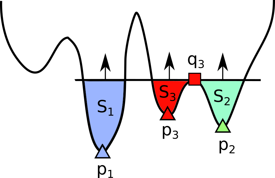
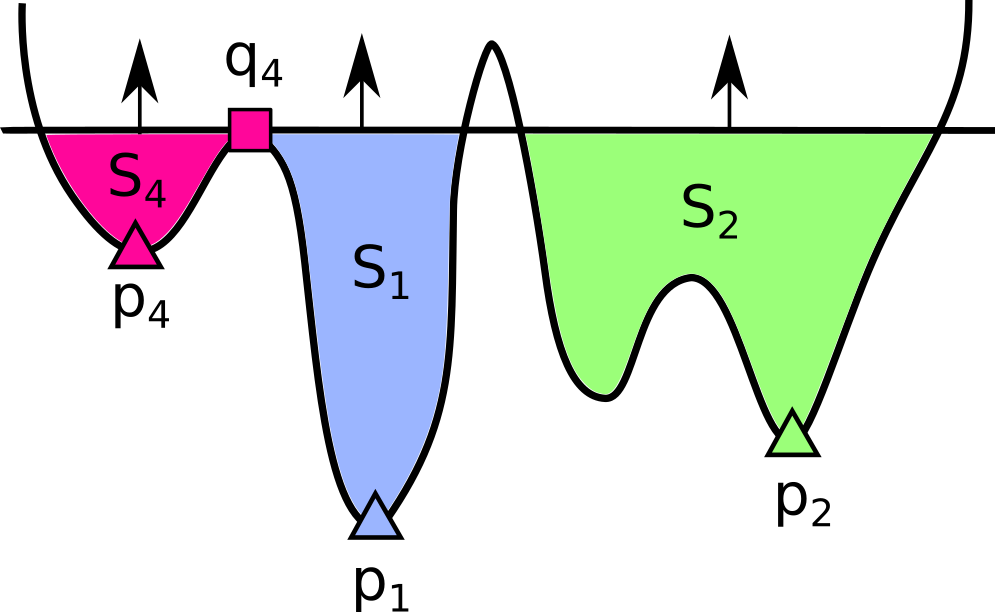
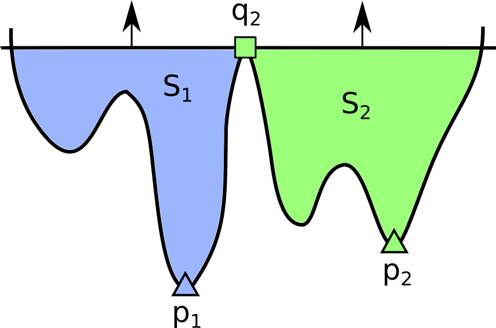
Connected components of sublevel sets merge at 1-saddle critical points.

A point $q$ is a 1-saddle critical point if the intersection of the set $\Theta_{f<f(q)}$ with any small neighborhood of $q$ has more than one connected components.

Let $p$ be a minimum, that is not global. When $c$ is increased sufficiently, the connected component of $\Theta_{f\leq c}$ born at $p$ merges with some other connected component. Then this unified connected component may merge again with another one. After each merging the minimum of the restriction of $f$ to the unified connected component is the smallest of the two minima of restriction of $f$ to each of the two connected components before merging. In other words, the connected component with lower minimum "swallows" at the merging point the connected component with higher minimum, see fig 1. Let $q$ be the merging point where connected component with minimum $p$ is swallowed by connected component whose minimum is lower. Note that the intersection of the set $\Theta_{f<f(q)}$ with any small neighborhood of $q$ has at least two connected components. The point $q$ is the 1-saddle associated naturally with the minimum $p$.

Note that the two connected components of the intersection of a small neighborhood of such $q$ with $\Theta_{f<f(q)}$ belong to two different connected components of the whole set $\Theta_{f<f(q)}$. The 1-saddles of this type are called “+” (“plus”) or “death” type. The described correspondence between local minima and 1-saddles of this type is one-to-one. This follows immediately for example from the definition 2 below.

In a similar way, the 1-saddle $q$ associated with $p$ can be described also as follows.

Proposition 2.1.

Consider various paths $\gamma$ starting from local minimum $p$ and going to a lower minimum. Let $m_{\gamma}\in\Theta$ is the maximum of the restriction of $f$ to such path $\gamma$. Then $1$-saddle $q$ corresponding to the local minimum $p$ in the barcode is the minimum over the set of all such paths $\gamma$ of the maxima $m_{\gamma}$:

$$q=\operatorname{arg}\bigg{[}\min_{\begin{subarray}{c}\gamma:[0,1]\rightarrow\Theta\\ \gamma(0)=p,\,f(\gamma(1))<f(p)\end{subarray}}\max_{t}f\big{(}\gamma(t)\big{)}\bigg{]}$$ (1)

Proof.

Let the connected component of local minimum $p$ merges with connected component of a lower minimum at the point $q$. Then there is a path in $\Theta_{f\leq f(q)}$ passing through $q$ and connecting $p$ with the lower minimum. The point $q$ is the maximum of the restriction of $f$ to such path. And there is no path in sublevel sets $\Theta_{f\leq c}$, $c<f(q)$ , that connects $p$ with a lower minimum. Therefore there is no path with $f(m_{\gamma})<f(q)$. ∎

Definition 2: New minimum on connected components of sublevel set

This is essentially a variant of the previous definition when looking at things from the perspective of the saddle.

The correspondence in the opposite direction can be described analogously. Let $q$ be a 1-saddle point of such type that the two branches of the set $\Theta_{f<f(q)}$ near $q$ are not connected in the whole set $\Theta_{f<f(q)}$. One of the connected components of the sublevel set $\Theta_{f\leq c}$ splits into two when $c$ decreases from $f(q)+\epsilon$ to $f(q)-\epsilon$. Let $p_{1}$ and $p_{2}$ are the two minima of the restriction of $f$ to each of these two connected components. Let $p_{1}>p_{2}$ is the highest of the two minima. The 1-saddle $q$ is associated with the local minimum $p_{1}$. Notice that $p_{1}$ did not appear as a minimum of $f$ on one of connected components of $\Theta_{f\leq f(q)+\epsilon}$. In other words $p_{1}$ is the new minimum appearing in the set of minima of $f$ on connected components of $\Theta_{f\leq c}$ when $c$ decreases from $f(q)+\epsilon$ to $f(q)-\epsilon$.

Proposition 2.2.

Given a 1-saddle $q$ as above, the minimum $p$ which corresponds to $q$ in the barcode is the new minimum appearing in the set of minima of $f$ on connected components of $\Theta_{f\leq c}$ when $c$ decreases from $f(q)+\epsilon$ to $f(q)-\epsilon$. ∎

The two branches of the set $\Theta_{f\leq f(q)-\epsilon}$ near $q$ can also belong to the same connected component of this set. Then such saddle is of “birth”, or "-" type and it is naturally coupled with 2-index saddle of “death” type, see Theorem 2.3 below.

Definition 3: Invariants of filtered complexes

We recall here the general definition for the full "canonical form" ("barcode") invariants from [2]. Although our algorithm from section 3 is based on definition 1, we need definition 3 below to put things into general framework in which these invariants constitute the full description of the objective function topology. The reader interested mainly in the algorithm and the calculations can safely skip this part.

Chain complex is the algebraic counterpart of intuitive idea representing complicated geometric objects as a decomposition into simple pieces. It converts such a decomposition into a collection of vector spaces and linear maps.

A chain complex $(C_{*},\partial_{*})$ is a sequence of finite-dimensional vector spaces $C_{j}$ (spaces of "$j-$chains") and linear operators ("differentials")

$$\rightarrow C_{j+1}\stackrel{{\scriptstyle\partial_{j+1}}}{{\rightarrow}}C_{j}\stackrel{{\scriptstyle\partial_{j}}}{{\rightarrow}}C_{j-1}\rightarrow\ldots\rightarrow C_{0},$$

which satisfy

$$\partial_{j}\circ\partial_{j+1}=0.$$

The image of the operator $\partial_{j+1}$ is a subspace in the kernel of the operator $\partial_{j}$. The $j-$th homology of the chain complex $(C_{*},\partial_{*})$ is the quotient of vector spaces

$$H_{j}=\ker\left(\partial_{j}\right)/\textrm{im}\left(\partial_{j+1}\right).$$

In many interesting situations the decomposition of complicated geometric object into simple pieces depends on some parameter or scale, then its algebraic counterpart is described by $\mathbb{R}-$filtered complex.

A subcomplex $(C^{\prime}_{*},\partial^{\prime}_{*})\subseteq(C_{*},\partial_{*})$ is a sequence of subspaces $C^{\prime}_{j}\subseteq C_{j}$ equipped with compatible differentials $\partial^{\prime}_{j}=\partial_{j}\mid_{C^{\prime}_{j}}$.

A chain complex $C_{*}$ is called $\mathbb{R}-$filtered if $C_{*}$ is equipped with an increasing sequence of subcomplexes ($\mathbb{R}-$filtration): $F_{s_{1}}C_{\ast}\subset F_{s_{2}}C_{*}\subset\ldots\subset F_{s_{max}}C_{*}=C_{*}$, indexed by a finite set of real numbers $s_{1}<s_{2}<\ldots<s_{\text{max}}$.

Theorem 2.3.

([2]) Any $\mathbb{R}-$filtered chain complex $C_{*}$ can be brought to “canonical form”, a canonically defined direct sum of $\mathbb{R}-$filtered complexes of two types: one-dimensional complexes with trivial differential $\partial_{j}(e_{i})=0$ and two-dimensional complexes with trivial homology $\partial_{j}(e_{i_{2}})=e_{i_{1}}$, by a linear transformation preserving the $\mathbb{R}-$filtration. The resulting canonical form is unique

The full barcode is a visualization of the decomposition of an $\mathbb{R}-$filtered complex according to the theorem 2.3. Each filtered 2-dimensional complex with trivial homology $\partial_{j}(e_{i_{2}})=e_{i_{1}}$, $\left\langle{e}_{i_{1}}\right\rangle=F_{\leq s_{1}}$,$\left\langle{e}_{i_{1}},{e}_{i_{2}}\right\rangle=F_{\leq s_{2}}$ describes a single topological feature in dimension $j$ which is "born" at $s_{1}$ and which "dies" at $s_{2}$. It is represented by segment $[s_{1},s_{2}]$ in the degree-$j$ barcode. And each filtered one-dimensional complex with trivial differential, $\partial_{j}{e}_{i}=0$ , $\left\langle{e}_{i}\right\rangle=F_{\leq r}$ describes a topological feature in dimension $j$ which is "born" at $r$ and never "dies". It is represented by the half-line $[r,+\infty[$ in the degree-$j$ barcode.

The proof of the theorem is given in Appendix 6.2. Essentially, one can bring an $\mathbb{R}-$filtered complex to the required canonical form by induction, starting from the lowest basis elements of degree one, in such a way that the manipulation of degree $j$ basis elements does not destroy the canonical form in degree $j-1$ and in lower filtration pieces in degree $j$.

Let $f:\Theta\to\mathbb{R}$ is smooth, or more generally, piece-wise smooth continuous function such that the sublevel sets $\Theta_{f\leq c}=\left\{\theta\in\Theta\mid f(\theta)\leq c\right\}$ are compact.

There are different filtered chain complexes computing the homology of the topological spaces $\Theta_{f\leq c}$ the Čech complexes, the simplicial complexes, or the CW-complexes.

Without loss of generality the function $f$ can be assumed smooth for the rest of this subsection, otherwise one can always replace $f$ by a smooth approximation. By adding a small perturbation we can also assume that critical points of $f$ are non-degenerate.

One filtered complex naturally associated with function $f$ and such that the subcomplexes $F_{s}C_{\ast}$ compute the homology of sublevel sets $\Theta_{f\leq s}$ is the gradient (Morse) complex, see section 6.1 or e.g. [2, 7, 26]. The gradient Morse complex is defined as follows. The basis elements in the $k-$vector spaces $C_{j}$ are in one-to-one correspondence with the critical points of $f$ of index $j$ equipped with a choice of orientation. The orientation here is a choice of orientation of $j$-dimensional subspace of tangent space at the critical point, on which the Hessian is negative defined. The matrix of $\partial_{j}$ consists of the numbers of gradient trajectories, counted with signs, between the index $j$ and the index $(j-1)$ critical points.

Proposition 2.4.

Let $p$ be a minimum, which is not global. The basis element corresponding to $p$ represents trivial homology class in the canonical form of the gradient Morse complex of $f$. Then $p$ is the lower basis element of one of the two-dimensional complexes with trivial homology in the canonical form. I.e. $p$ is coupled with a 1-index saddle $q$ in the canonical form. This is the 1-saddle from definition 1, i.e. $q$ is the 1-saddle at which the sublevel set connected component corresponding to $p$ is swallowed by a connected component with lower minimum. The segment $\left[f(p),f(q)\right]$ is then the canonical invariant (barcode) corresponding to the minimum $p$.

Proof.

Let $q$ be the 1-saddle at which the connected component corresponding to $p$ is swallowed by a connected component with lower minimum $r$. The homology $H_{0}(\Theta_{f\leq f(q)-\epsilon})$ are generated linearly by classes of connected components of $\Theta_{f\leq f(q)-\epsilon}$. They correspond to the generators of the Morse complex given by minima of restriction of $f$ to each connected component. In the Morse complex computing homology of $\Theta_{f\leq f(q)+\epsilon}$ , the generator corresponding to the local minimum $p$ equals to the boundary of the generator corresponding to the 1-saddle $q$ plus the generator corresponding to the lower minimum $r$ plus perhaps boundaries of lower than $q$ saddles. Therefore $q$ is coupled with $p$ in the canonical form. ∎

The full canonical form of the gradient (Morse) complex of all indexes is a summary of global structure of the objective function’s gradient flow.

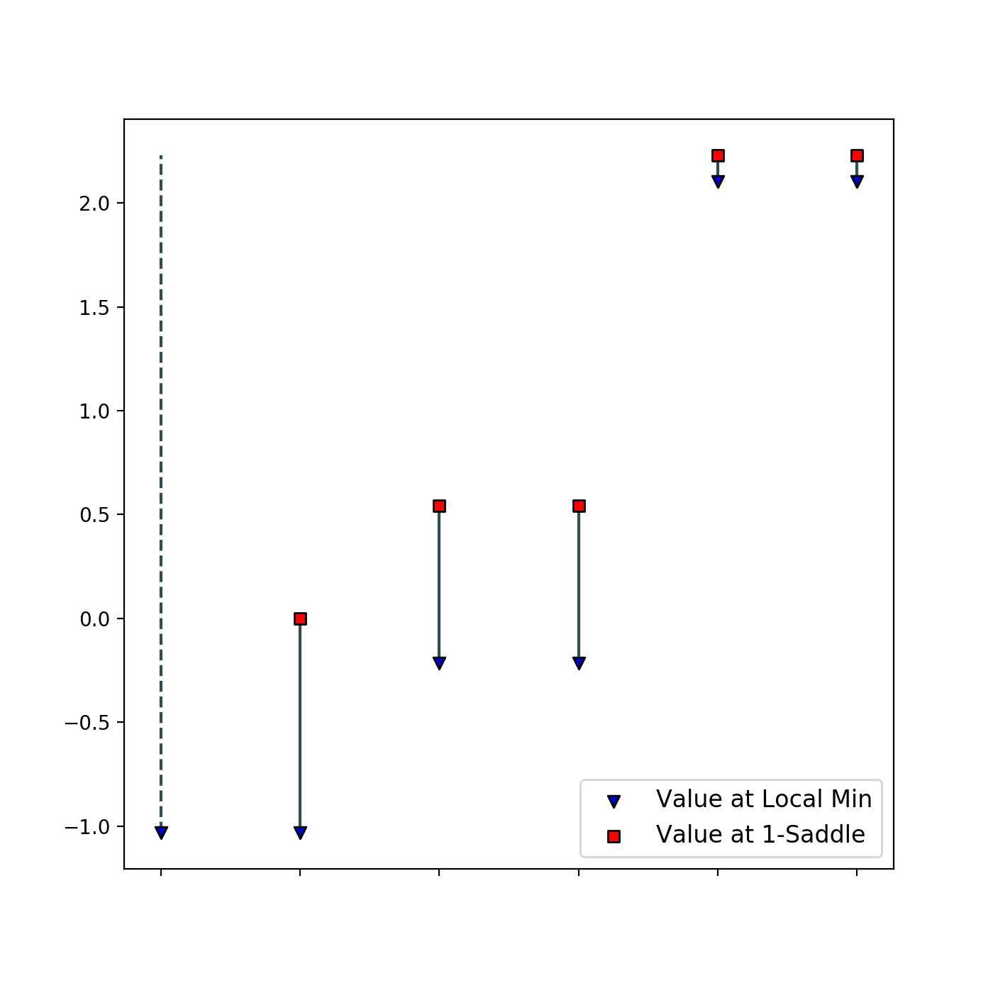
The total number of different topological features in sublevel sets $\Theta_{f\leq c}$ of the objective function can be read immediately from the barcode. Namely the number of intersections of horizontal line at level $c$ with segments in the index $j$ barcode gives the number of independent topological features of dimension $j$ in $\Theta_{f\leq c}$, see e.g. section 4.1.1.

3 An Algorithm for Calculation of Barcodes of Minima

In this section we describe our algorithm for calculation of the canonical form invariants of local minima. The algorithm uses definition 1 of barcodes from Section 2 that is based on the evolution on the connected components of the sublevel sets.

To analyse the surface of the given function $f:\Theta\rightarrow\mathbb{R}$, we first build its approximation by finite graph-based construction. To do this, we consider a randomly sampled subset of points $\{\theta_{1},\ldots,\theta_{N}\}\in\Theta$ and construct a graph with these points as vertices. We connect vertices with an edge if the points are close. Thus, for every vertex $\theta_{n}$, by comparing $f(\theta_{n})$ with $f(\theta_{n^{\prime}})$ for neighbors $\theta_{n^{\prime}}$ of $\theta_{n}$, we are able to understand the local topology near the point $\theta_{n}$. At the same time, connected componets of sublevel sets $\Theta_{f\leq c}$ naturally correspond to connected components of the subgraph $\Xi_{f\leq c}$ of points $\theta_{n}$, such that $f(\theta_{n})\leq c$.

Two technical details here are the choice of points $\theta_{n}$ and the definition of closeness, i.e. when to connect points by an edge. In our experiments, we sample points uniformly from some rectangular box of interest. To add edges, we compute the oriented $k$-nearest neighbor graph on the given points, then drop the orientation of edges and check that the distance between neighbors does not exceed $c(D)N^{-\frac{1}{D}}$, where $D$ is the dimension of $f$’s input. We use $k=2D$ in our experiments

We describe now our algorithm that computes barcodes of a function from its graph-based approximation described above. The key idea is to monitor the evolution of the connected components of the sublevel sets of the graph $\Xi_{f\leq c}=\{\theta_{n}\text{ | }f(\theta_{n})\leq c\}$ for increasing $c$.

Input :  Undirected graph $G=(V,E)$; function $f$ on graph vertices.

Output :  Barcodes: a list of "birth"-"death" pairs.

$S\leftarrow\{\}$;

for $\theta\in V\text{ in increasing order of }f(\theta)$ do

       $S^{\prime}\leftarrow\{s\in S\text{ | }\exists\theta^{\prime}\in s\text{ such that }(\theta,\theta^{\prime})\in E\text{ and }f(\theta)>f(\theta^{\prime})\}$;

       if $S^{\prime}=\emptyset$ then

             $S\leftarrow S\sqcup\{\{\theta\}\}$;

            

       else

             $f^{*}\leftarrow\min f(\theta^{\prime})$ for $\theta^{\prime}\in\bigsqcup\limits_{s\in S^{\prime}}s$;

             for $s\in S^{\prime}$ do

                   $f^{s}\leftarrow\min f(\theta^{\prime})$ for $\theta^{\prime}\in s$;

                   if $f^{s}\neq f^{*}$ then

                         $\text{Barcodes}\leftarrow\text{Barcodes}\sqcup\{\big{(}f^{s},f(\theta)\big{)}\}$;

                        

                  

             end for

            $s_{\text{new}}\leftarrow\big{(}\bigsqcup\limits_{s\in S^{\prime}}s\big{)}\sqcup\{\theta\}$;

             $S\leftarrow(S\setminus S^{\prime})\sqcup\{s_{\text{new}}\}$;

            

       end if

      

end for

for $s\in S$ do

      $f^{s}\leftarrow\min f(\theta^{\prime})$ for $\theta^{\prime}\in s$;

       $\text{Barcodes}\leftarrow\text{Barcodes}\sqcup\{\big{(}f^{s},\infty\big{)}\}$;

      

end for

return Barcodes

Algorithm 1 Barcodes of minima computation for function on a graph.

For simplicity we assume that points $\theta$ are ordered w.r.t. the value of function $f$, i.e. for $n<n^{\prime}$ we have $f(\theta_{n})<f(\theta_{n^{\prime}})$. In this case we are interested in the evolution of connected components throughout the process of sequential adding of vertices $\theta_{1},\theta_{2},\dots,\theta_{N}$ to graph, starting from an empty graph. We denote the subgraph on vertices $\theta_{1},\dots,\theta_{n}$ by $\Xi_{n}$. When we add new vertex $\theta_{n+1}$ to $\Xi_{n}$, there are three possibilities for connected componenets to evolve:

• Vertex $\theta_{n+1}$ has zero degree in $\Xi_{n+1}$. This means that $\theta_{n+1}$ is a local minimum of $f$ and it forms a new connected component in the sublevel set.

• All the neighbors of $\theta_{n+1}$ in $\Xi_{n+1}$ belong to one connected component in $\Xi_{n}$.

• All the neighbors of $\theta_{n+1}$ in $\Xi_{n+1}$ belong to $K\geq 2$ connected components ${s_{1},s_{2},\dots,s_{K}\subset\Xi_{n}}$. Thus, all these components will form a single connected component in $\Xi_{n+1}$.

In the third case, according to definition 1 of section 2, the point $\theta_{n+1}$ is a discrete $1$-saddle point. Thus, one of the components $s_{k}$ swallows all the rest. This is the component which has the lowest minimal value. For other components, this gives their barcodes: for $s_{i},i\neq k$ the birth-death pair is $\big{[}\min\limits_{\theta\in s_{i}}f(\theta);f(\theta_{n+1})\big{]}$. We summarize the procedure in the algorithm 1.

In the practical implementation of the algorithm, we precompute the values of function $f$ at the vertices of $G$. Besides that, we use the disjoint set data structure to store and merge connected components during the process. We also keep and update the global minima in each component. We did not include these tricks into the algorithm’s pseuso-code in order to keep it simple.

The resulting complexity of the algorithm is $O(N\log N)$ in the number of points. Here it is important to note that the procedure of graph creation may be itself time-consuming. In our case, the most time consuming operation is nearest neighbor search. In our code, we used efficient HNSW Algorithm for aproximate NN search by [21]. Also since we only take neighbors lying no further than fixed small distance $r=O(N^{-\frac{1}{D}})$, one can use the following simple strategy as well. First, distribute points from the sample over boxes of fixed grid with edges of size $\frac{1}{2}r$. Then, in order to determine the neighbors, check distances from each point to the points lying only in the neighboring boxes of the grid.

4 Experiments

In this section we apply our algorithm to describing the topology of test functions. In subsection 4.1 we apply the algorithm to visual examples and check the convergence on benchmark functions. In subsection 4.2 we apply our algorithm to analyse the loss surfaces of small neural networks.

4.1 Barcodes of benchmark functions and convergence of the algorithm

In this subsection we apply our algorithm to several functions ${f:\mathbb{R}^{D}\rightarrow\mathbb{R}}$ from Global Optimization Benchmark [15]. These functions are designed to fool global optimization algorithms, they are very complex, have many local minima and saddle points even for small dimensions. Thus, the computation of barcodes and minimum-saddle correspondence for these functions is also non-trivial. In particular, it requires finding the global minimum.

4.1.1 Barcodes of 2D benchmark functions

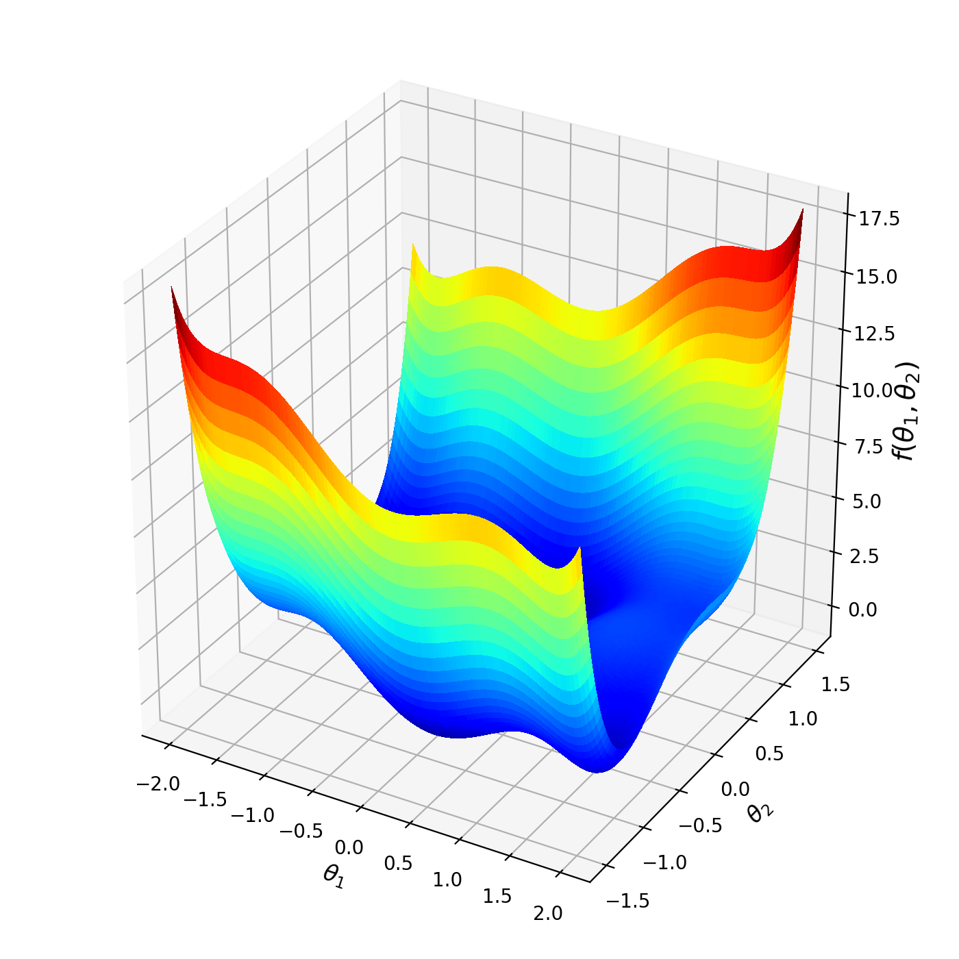
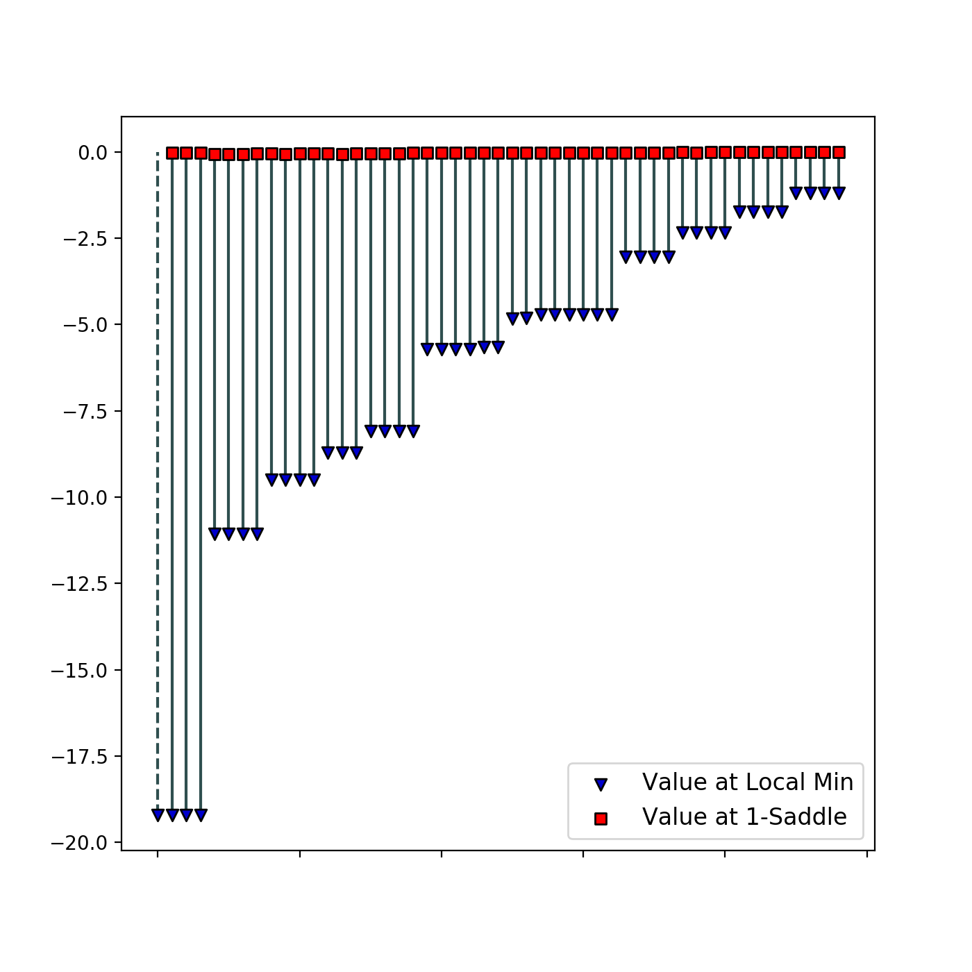
To begin with, we compute barcodes of several $2$-dimensional benchmark functions. We visualise obtained barcodes and minima-saddles correspondence. Next, we conduct the experiments to estimate how the number of points used to compute barcodes influences the quality of the answer. We consider the following test objective functions:

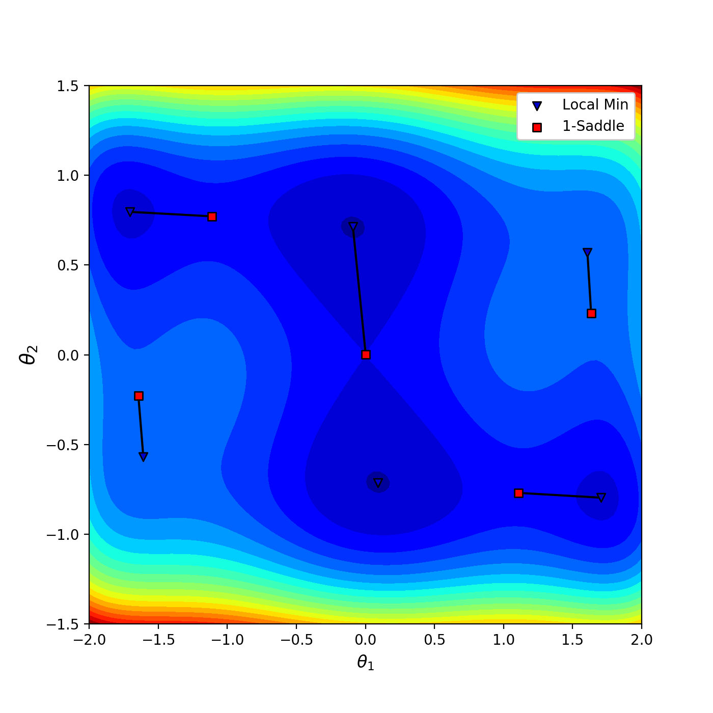
1. HumpCamel6 function $f:[-2,2]\times[-1.5,1.5]\rightarrow\mathbb{R}$ with 6 local minima (Figure 2):

   $$f(\theta_{1},\theta_{2})=(4-2.1\theta_{1}^{2}+\theta_{1}^{4}/3)\theta_{1}^{2}+\theta_{1}\theta_{2}+(-4+4\theta_{2}^{2})\theta_{2}^{2}$$

(a) Surface plot (3D).

(b) Color plot (2D) & correspondence between minima and 1-saddle points.

(c) Barcode of local minima.

Figure 2: HumpCamel6 function, its minima-saddle correspondence and barcode computed by Algorithm 1.

(a) Surface plot (3D).

(b) Color plot (2D) & correspondence between minima and 1-saddle points.

(c) Barcode of local minima.

Figure 3: Langermann function, its minima-saddle correspondence and barcodes computed by Algorithm 1.

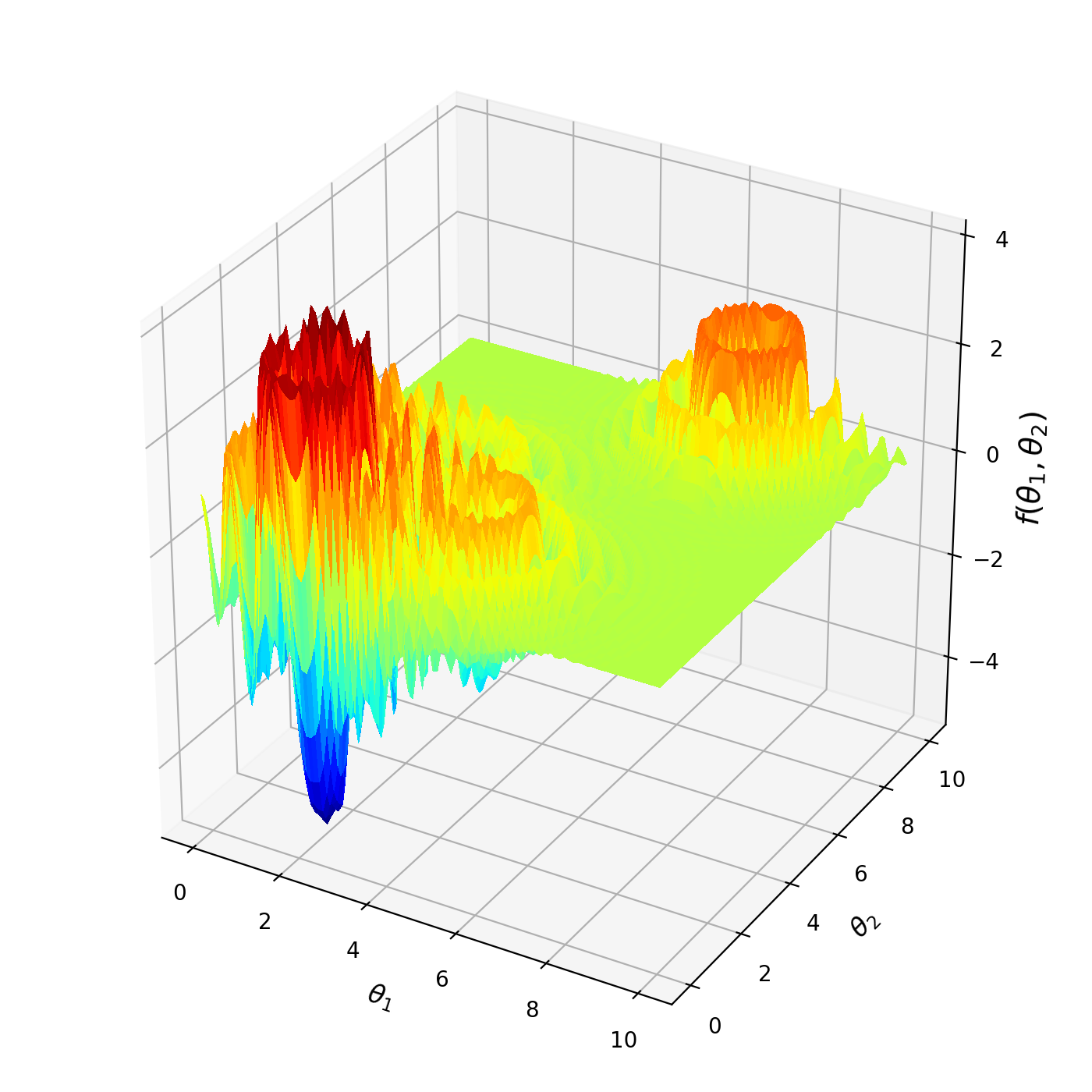
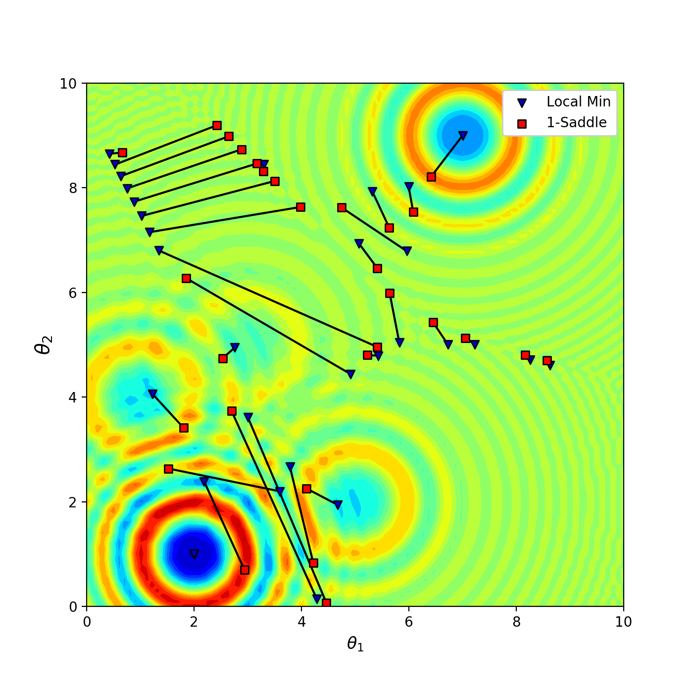
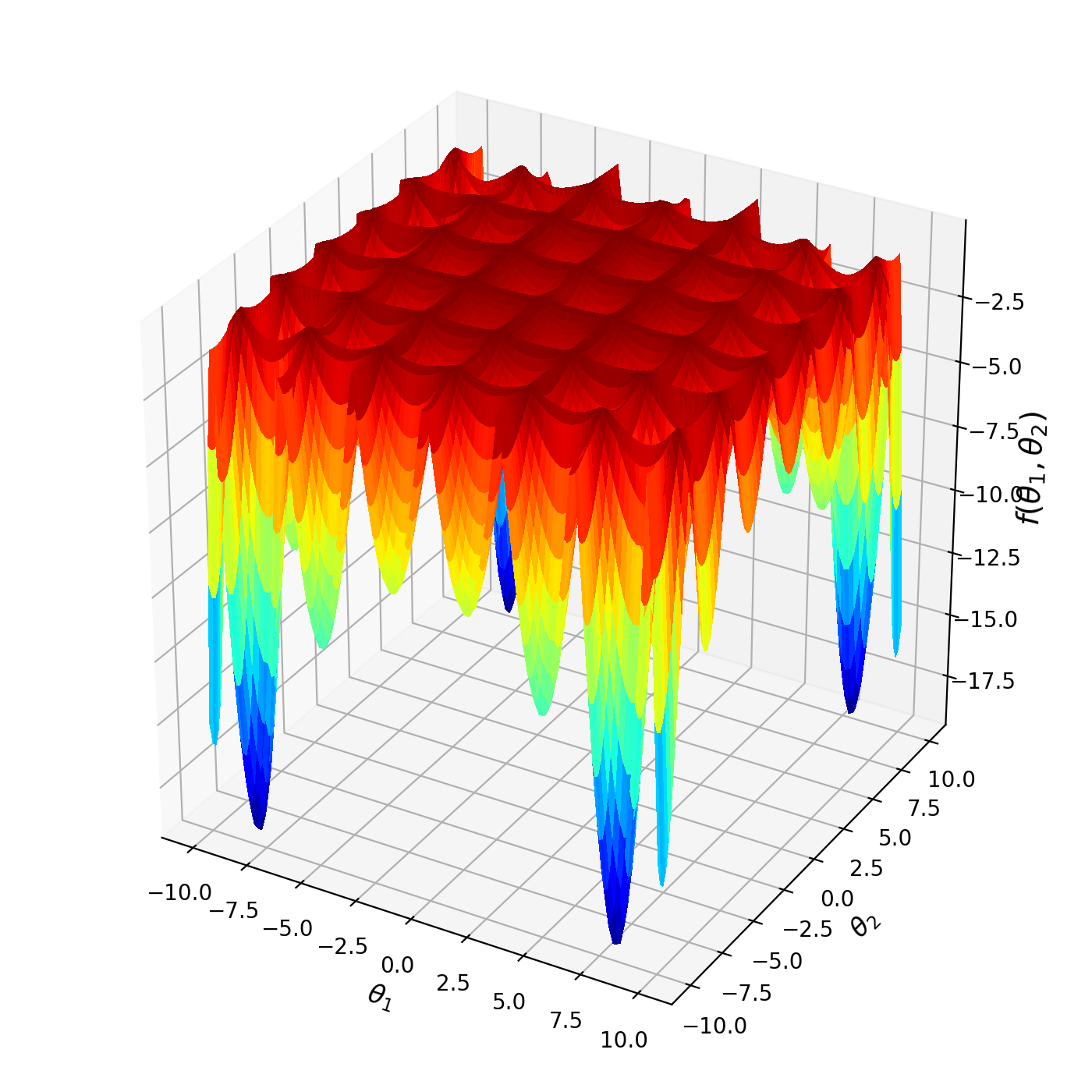
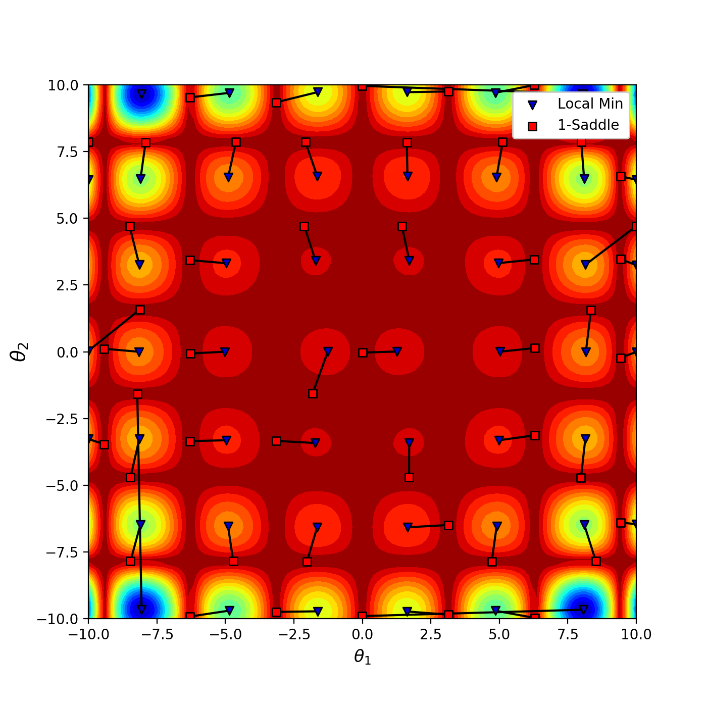
1. Langermann test objective function $f:[0,10]^{2}\rightarrow\mathbb{R}$ (Figure 3):

   $$f(\theta_{1},\theta_{2})=-\sum_{i=1}^{5}\frac{c_{i}\cos\big{(}\pi\big{[}(\theta_{1}-a_{i})^{2}+(\theta_{2}-b_{i})^{2}\big{]}\big{)}}{e^{\frac{(\theta_{1}-a_{i})^{2}+(\theta_{2}-b_{i})^{2}}{\pi}}}.$$

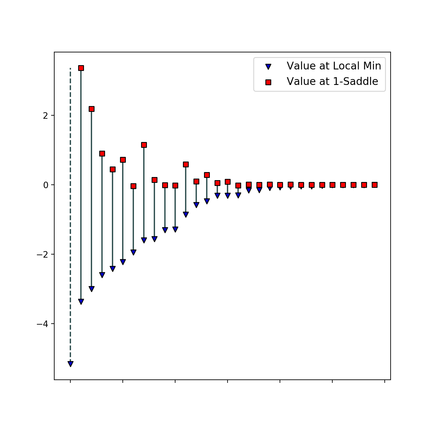
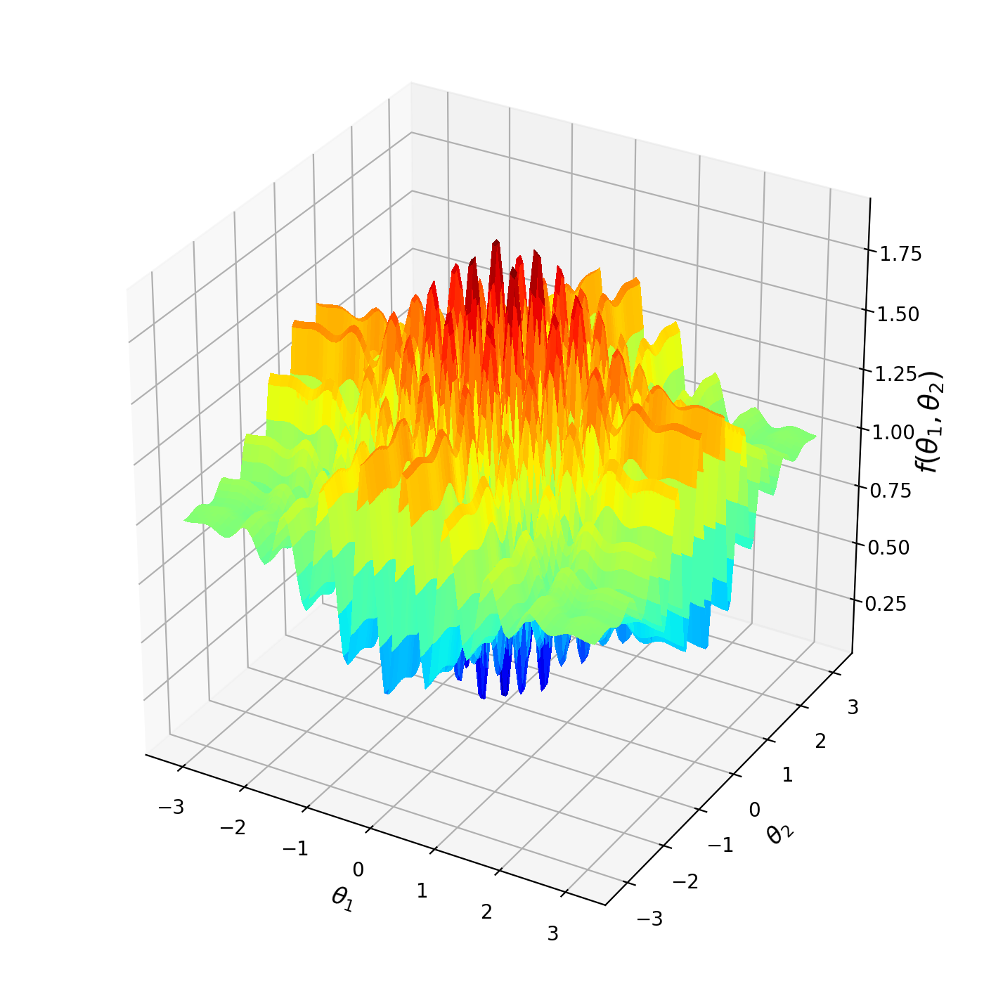
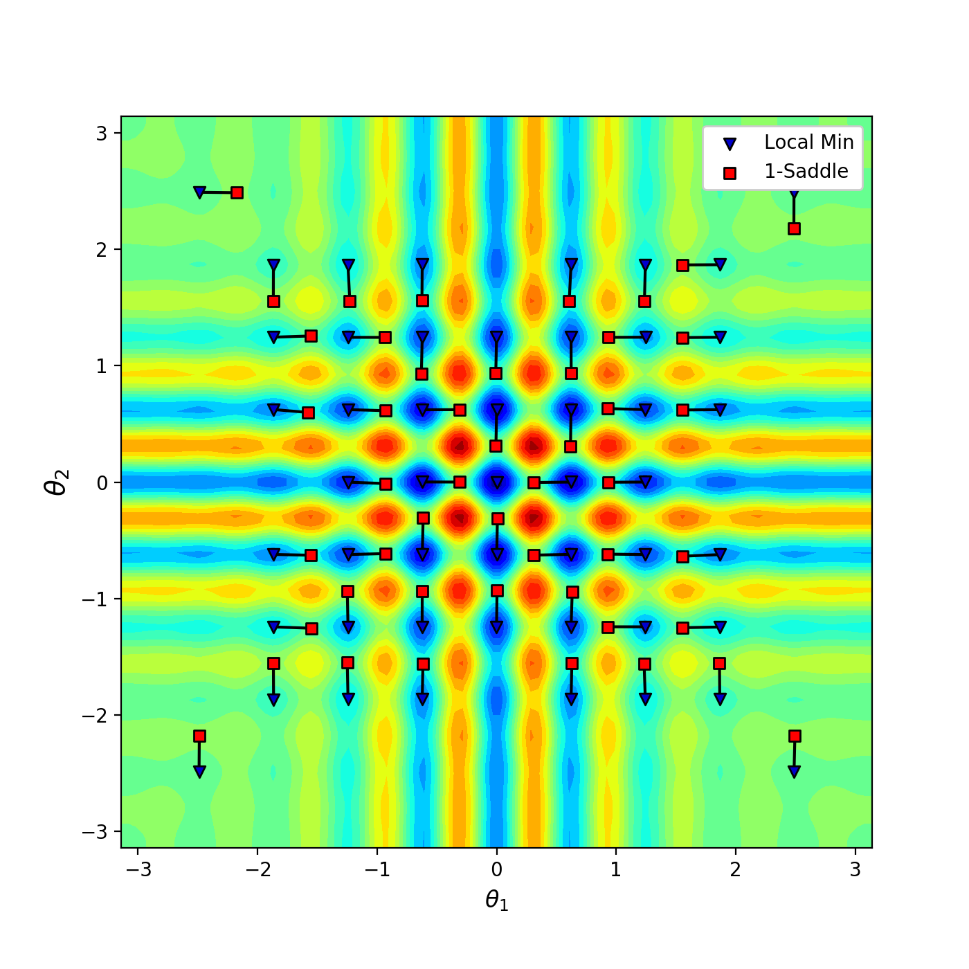
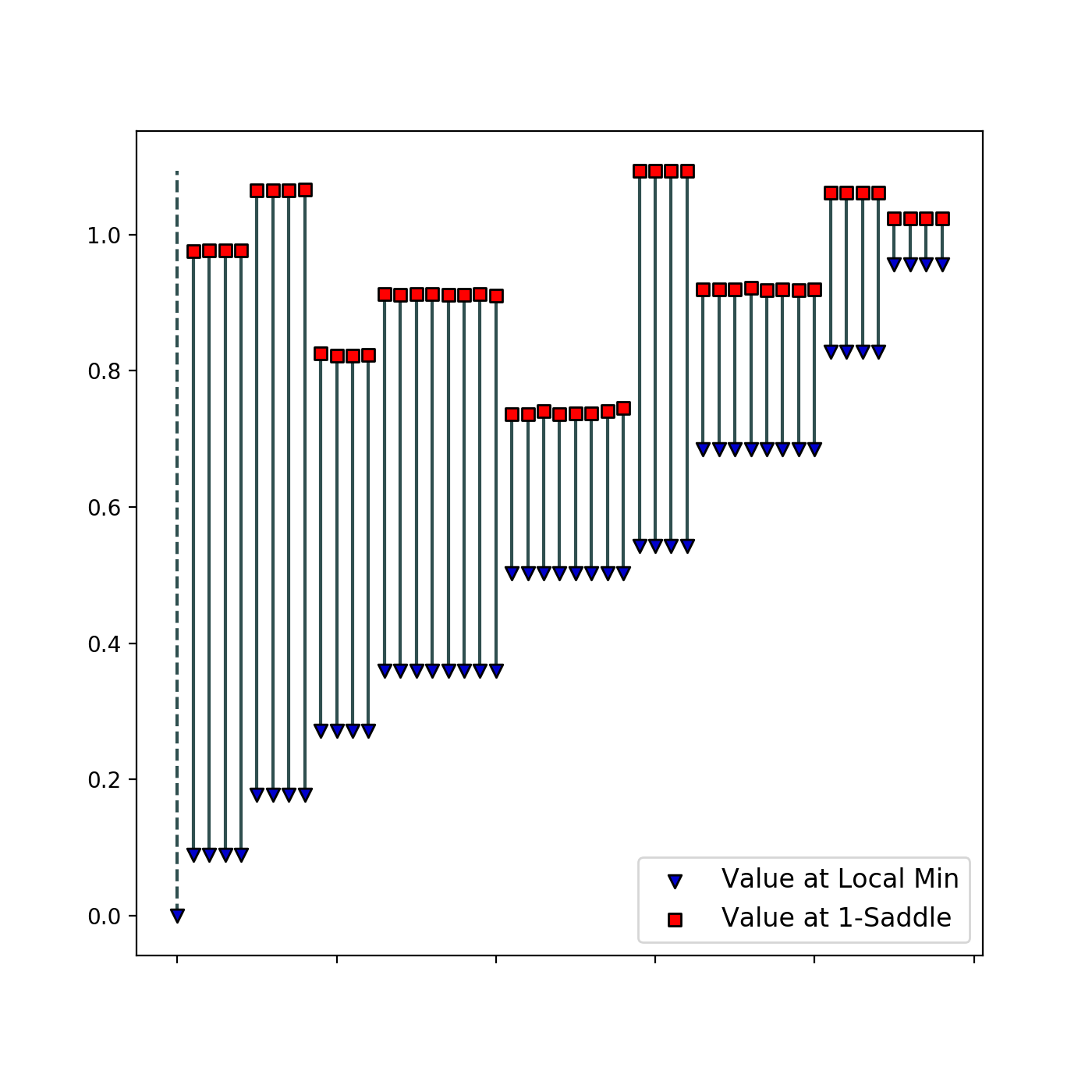
   To keep the plots simple, we displayed minimum-saddle correspondence only for Top-30 segments in barcode sorted by the size of the cluster (number of points at the cluster death moment). As wee see in Figure 3b, the correspondence between minimum-saddle is non-trivial. For many minima, the corresponding saddles are rather distant. In particular, this observation illustrates the remark discussed in Figure 1: the corresponding canonical $1$-saddle is not necessarily the nearest saddle.

1. Wavy test objective function $f:[-\pi,\pi]^{2}\rightarrow\mathbb{R}$ (Figure 4):

   $$f(\theta_{1},\theta_{2})=1-\frac{1}{2}\sum_{d=1}^{2}\cos(10\,\theta_{d})\cdot e^{-\frac{\theta_{d}^{2}}{2}},$$

   Wavy function is symmetric with respect to the dihedral group $D_{4}$ of order $8$. Thus, its minimum-saddle critical value pairs come in multiplets forming simple representations of the group $D_{4}$ (see [4] for more details on the equivariant barcodes).

(a) Surface plot (3D).

(b) Color plot (2D) & correspondence between minima and 1-saddle points.

(c) Barcode of local minima.

Figure 4: Wavy function, its minimum-saddle correspondence and barcode computed by Algorithm 1

1. HolderTable test objective function $f:[-10,10]^{2}\rightarrow\mathbb{R}$ (Figure 5):

   $$f(\theta_{1},\theta_{2})=-\left|e^{|1-\frac{\sqrt{\theta_{1}^{2}+\theta_{2}^{2}}}{\pi}|}\sin(\theta_{1})\cos(\theta_{2})\right|$$

(a) Surface plot (3D).

(b) Color plot (2D) & correspondence between minima and 1-saddle points.

(c) Barcode of local minima.

Figure 5: HolderTable function, its minimum-saddle correspondence and barcode computed by Algorithm 1

4.1.2 Convergence of the Algorithm

In this section we prove and test empirically the convergence of our algorithm when the number of points $N$ used to construct barcodes tends to infinity. To compare two barcodes we adopt Bottleneck distance [22, 16] (also known as Wasserstein-$\infty$ distance $\mathbb{W}_{\infty}$) on the corresponding persistence diagrams ($2$-dimensional point clouds of birth-death pairs):

$$\mathbb{W}_{\infty}(\mathcal{D},\mathcal{D}^{\prime}):=\inf_{\pi\in\Gamma(\mathcal{D},\mathcal{D}^{\prime})}\sup_{a\in\mathcal{D}\cup\Delta}\lvert a-\pi(a)\rvert.$$ (2)

Here $\Delta$ denotes the "diagonal" (pairs with birth equal to death) and $\Gamma(\mathcal{D},\mathcal{D}^{\prime})$ denotes the set of partial matchings between $\mathcal{D}$ and $\mathcal{D}^{\prime}$ defined as bijections between $\mathcal{D}\cup\Delta$ and $\mathcal{D}^{\prime}\cup\Delta$.

For a function $f:\Theta\rightarrow\mathbb{R}$ let $\mathcal{D}_{f}^{*}$ denote its barcode. Our algorithm uses finite number of $N$ randomly sampled points $\Theta_{N}=\{\theta_{1},\dots,\theta_{N}\}$ to compute approximation $\hat{\mathcal{D}}_{f}(\Theta_{N})$ of true barcode $\mathcal{D}_{f}^{*}$. Let $C$ denotes the Lipschitz constant of $f$

Proposition 4.1.

Let for any $\theta\in\Theta$ there exists $\theta_{i}\in\Theta_{N}$ such that $\lvert\theta-\theta_{i}\rvert<\varepsilon$. Then

$$\mathbb{W}_{\infty}\big{(}\hat{\mathcal{D}}_{f}(\Theta_{N}),\mathcal{D}_{f}^{*})\big{)}<C\varepsilon$$

Proof.

This follows from, e.g., ([10], Lemma 1). ∎

Note that for typical sample $\Theta_{N}$ the maximal distance from $\theta\in\Theta$ to $\Theta_{N}$ is $\sim N^{-\frac{1}{D}}$. It follows that $\hat{\mathcal{D}}_{f}(\Theta_{N})$ converges to $\mathcal{D}_{f}^{*}$ as $N\to\infty$ for any typical sequence of samples $\{\Theta_{N}\}$. And in particular

$$\mathbb{W}_{\infty}\big{(}\hat{\mathcal{D}}_{f}(\Theta_{N}),\hat{\mathcal{D}}_{f}(\Theta_{N}^{\prime})\big{)}\to 0$$ (3)

as $N\to\infty$, for any typical pair of sequences $\{\Theta_{N}\},\{\Theta_{N}^{\prime}\}$.

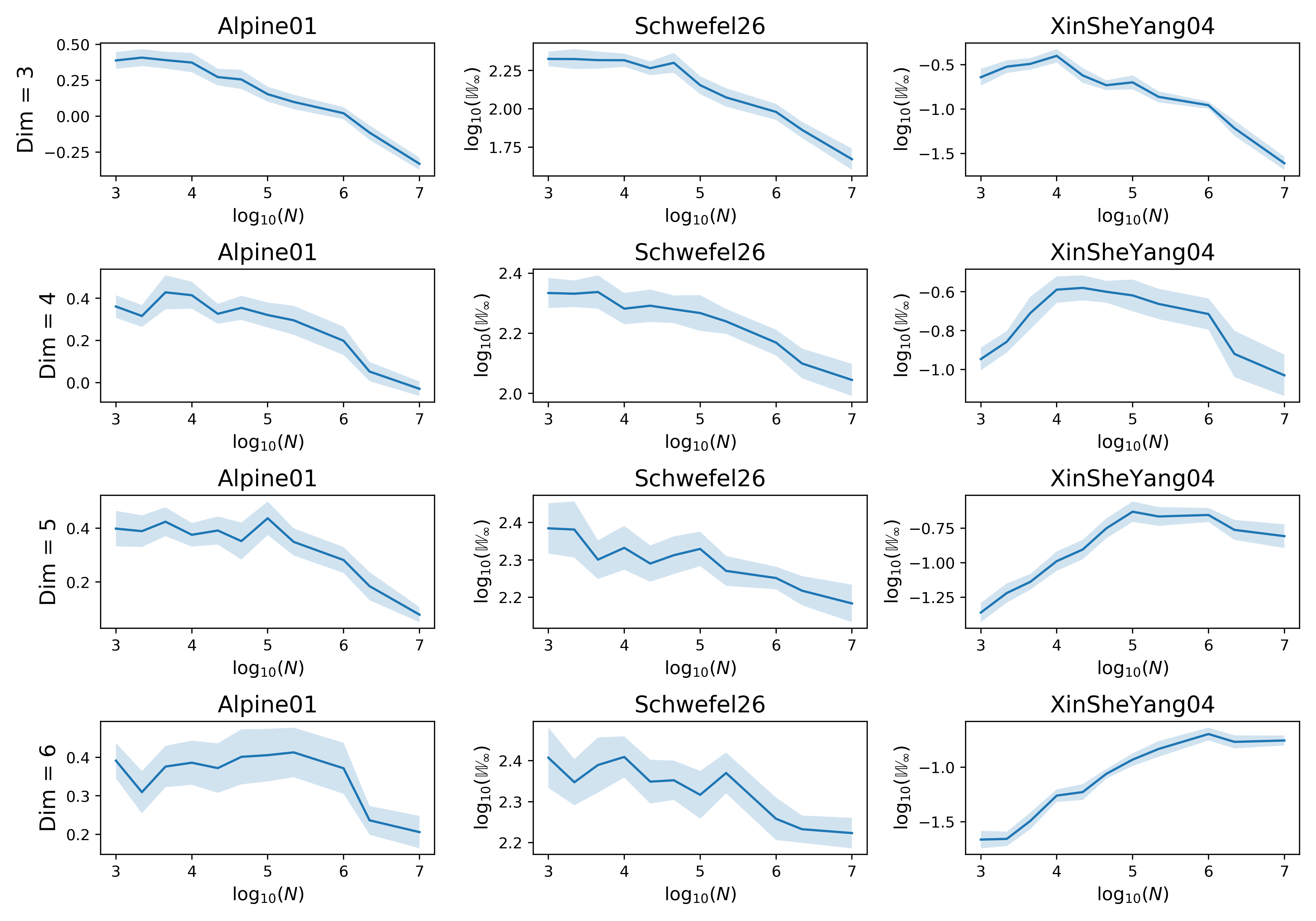
We have checked the condition (3) on several test function from Global Optimization benchmark. Each of the test function comes in a series of functions of arbitrary dimension. Even for small dimensions they are extremely complex (contain exponential number of local minima and saddle points). For each function $f$ and dimension $D=3,4,5,6$, we consider various sample sizes $\log_{10}N\in[3,3.5,4,\dots,7]$. For every triplet $(f,D,N)$, we randomly sample $R=20$ pairs $\big{(}(\Theta_{N})_{r},(\Theta_{N}^{\prime})_{r}\big{)}$ of point clouds of size $N$. Next for each of $2R$ point clouds we compute the barcode by our algorithm and in each pair measure the bottleneck distance between the barcodes. Finally, we take the mean value

$$\mathbb{E}_{\Theta_{N},\Theta_{N}^{\prime}}\mathbb{W}_{\infty}\big{(}\hat{\mathcal{D}}_{f}(\Theta_{N}),\hat{\mathcal{D}}_{f}(\Theta_{N}^{\prime})\big{)}\approx\frac{1}{R}\sum_{r=1}^{R}\mathbb{W}_{\infty}\big{(}\hat{\mathcal{D}}_{f}((\Theta_{N})_{r}),\hat{\mathcal{D}}_{f}((\Theta_{N}^{\prime})_{r})\big{)}.$$ (4)

The considered functions are:

1. Alpine01 function $f:[-10,10]^{D}\rightarrow\mathbb{R}$ defined by

   $$f(\theta_{1},\dots,\theta_{D})=\sum_{d=1}^{D}|\theta_{d}\sin\theta_{x_{d}}+0.1\theta_{d}|.$$

2. Schwefel26 function $f:[-500,500]^{D}\rightarrow\mathbb{R}$ defined by:

   $$f(\theta_{1},\dots,\theta_{D})=418.9829\cdot D-\sum_{d=1}^{D}\theta_{d}\sin(\sqrt{|\theta_{d}|}).$$

3. XinSheYang04 function $f:[-10,10]^{D}\rightarrow\mathbb{R}$ defined by:

   $$f(\theta_{1},\dots,\theta_{D})=\left[\sum_{d=1}^{D}\sin^{2}(\theta_{d})-e^{-\sum_{d=1}^{D}\theta_{d}^{2}}\right]e^{-\sum_{d=1}^{D}\sin^{2}\sqrt{\lvert\theta_{d}\rvert}}$$

For every pair $(f,D)$ we sum up the dependence on $N$ in a form of a plot in the decimal logarithmic scale. We observe empirically that for big enough $N$

$$\log(\mathbb{W}_{\infty}\big{(}\hat{\mathcal{D}}_{f}(\Theta_{N}),\hat{\mathcal{D}}_{f}(\Theta_{N}^{\prime})\big{)})\sim-\frac{1}{D}\log(N)$$

as it is expected based on proposition 4.1.

The results are summarized in the following Figure 6.

Figure 6: Dependence of Bottleneck distance between pairs of persistent diagrams on the sample size $N$ for Alpine01, Schwefel26, XinSheYang04 function in dimensions $D\in\{3,4,5,6\}$.

4.2 Topology of neural network loss function

(a) Barcodes for ($2$) net

(b) Barcodes for ($3$) net

(c) Barcodes for ($2\times 2$) net

(d) Barcodes for ($3\times 2$) net

(e) Barcodes for ($3\times 3$) net

(f) Barcodes for ($2\times 2\times 2$) net

(g) Barcodes for ($3\times 2\times 2$) net

Figure 7: Barcodes of different neural network loss surfaces.

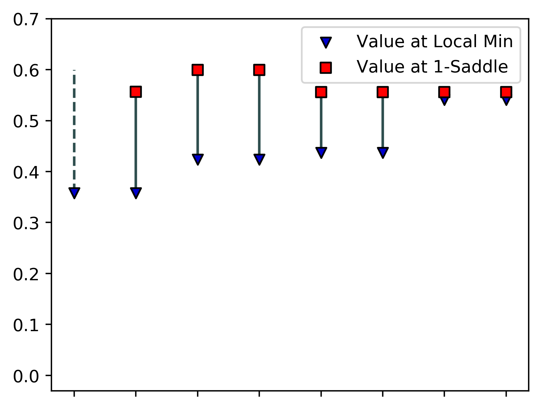
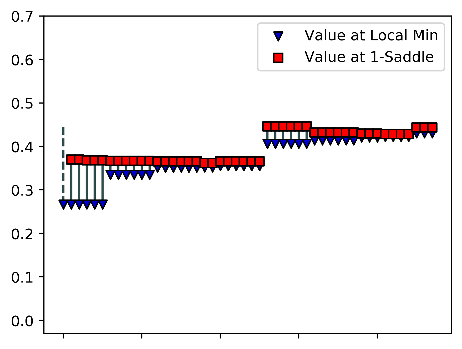
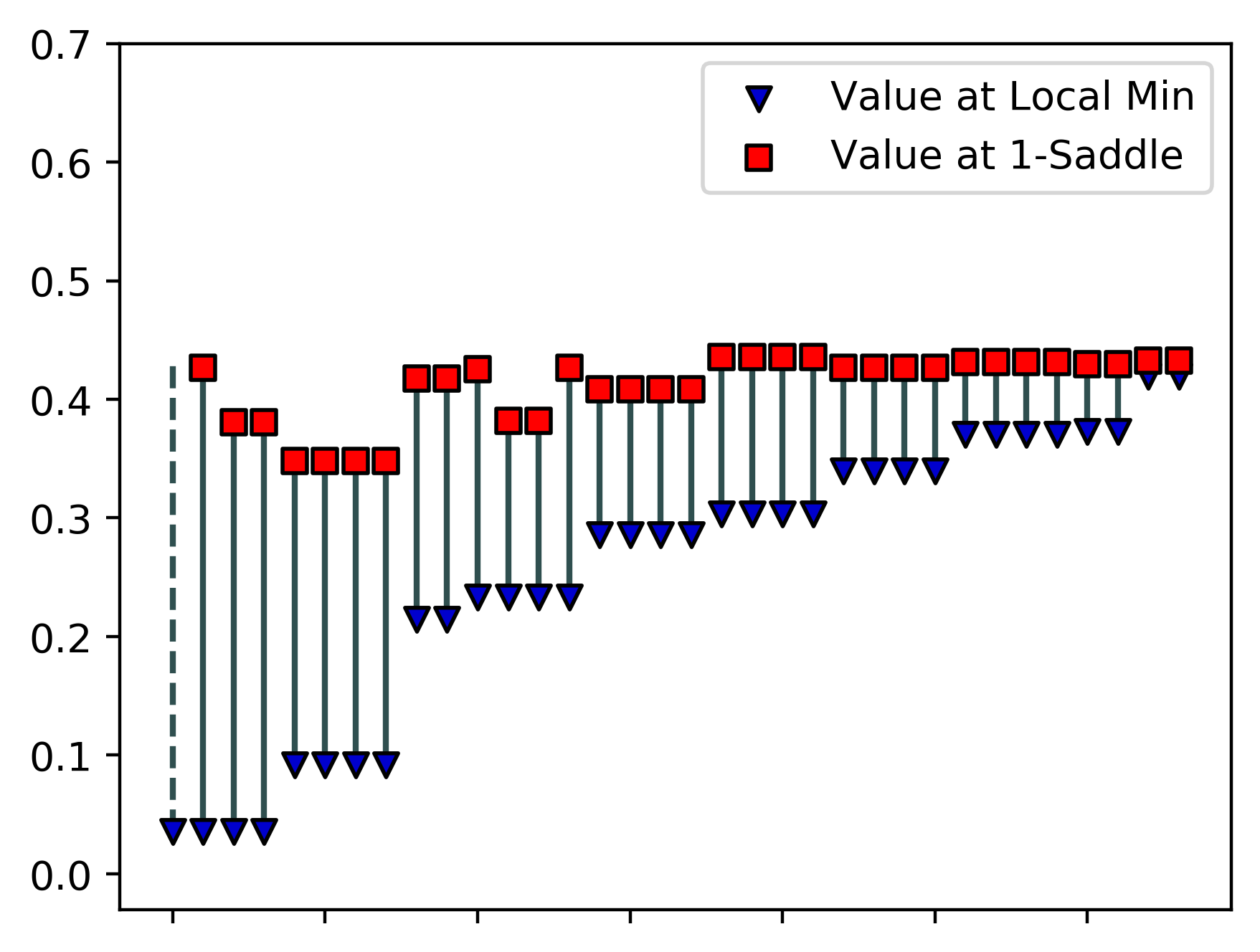
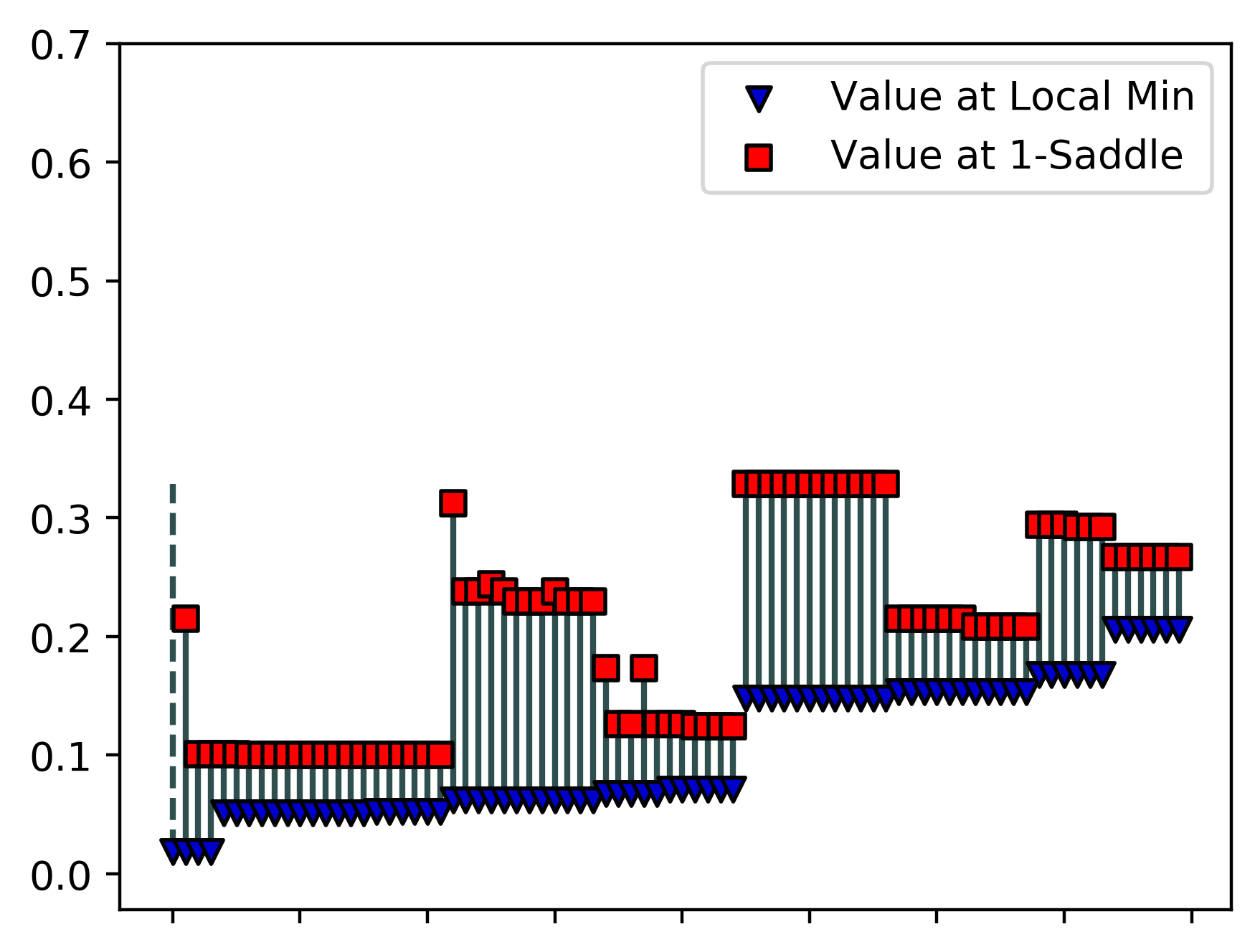
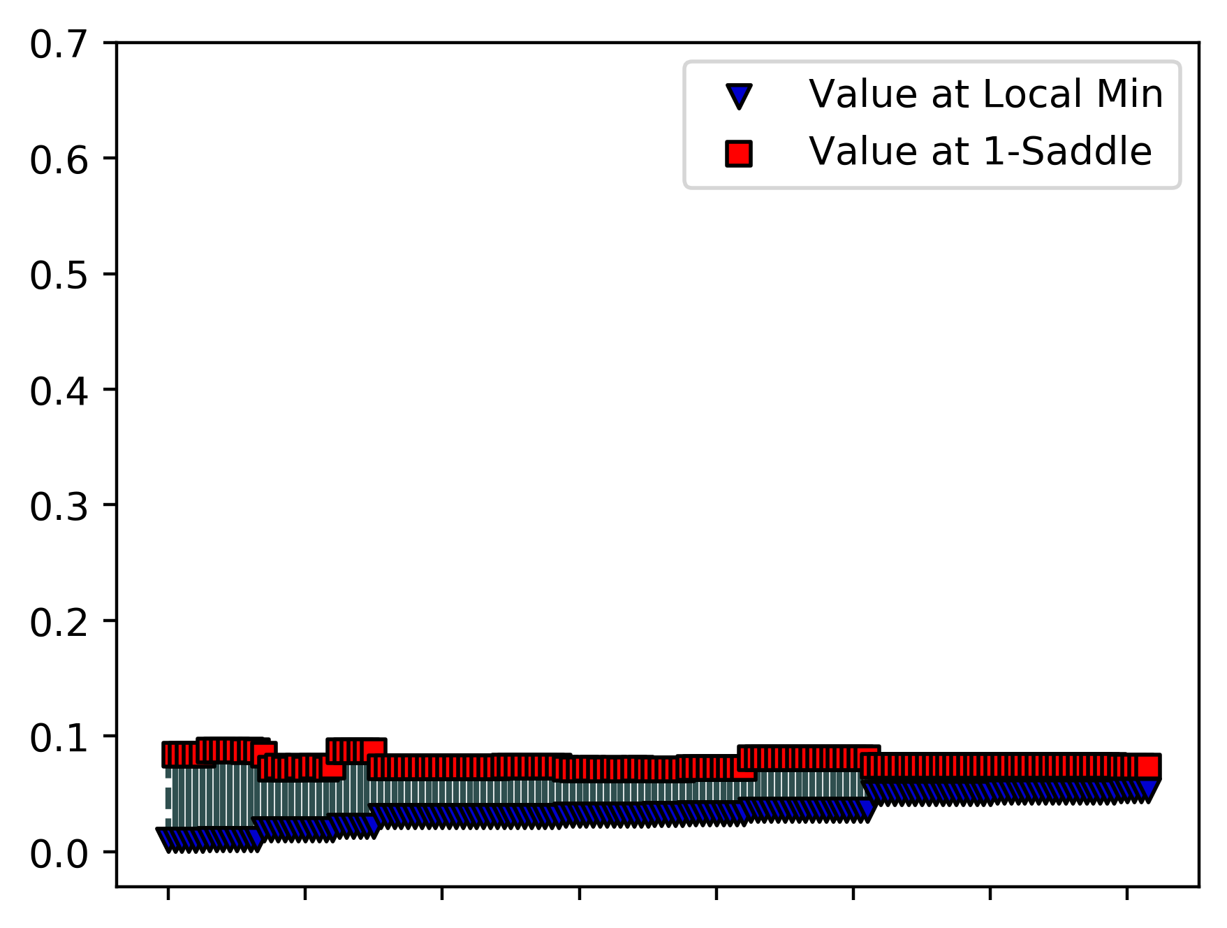
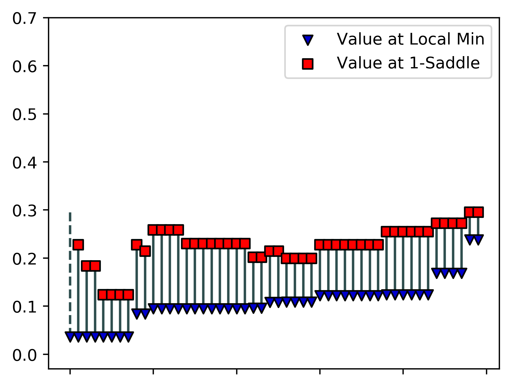
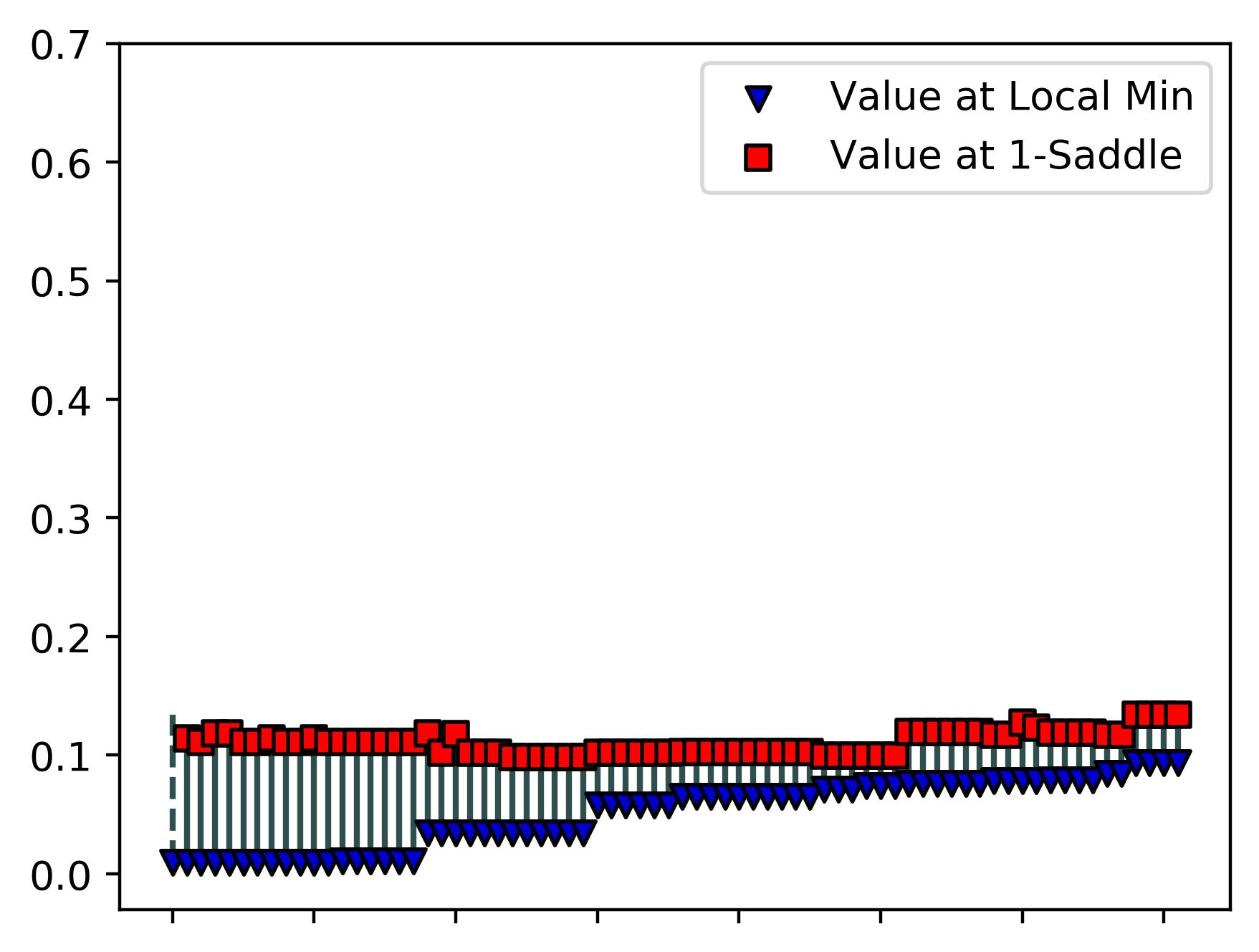
In this section we compute and analyse barcodes of small fully connected neural networks with up to three hidden layers.

For several architectures of the neural networks many results on the loss surface and its local minima are known (see e.g. [17, 14] and references therein). Different geometrical and topological properties of loss surfaces were studied in [8, 30, 9, 13].

There is no ground truth on how should the best loss surface of a neural network looks like. Nevertheless, there exists many common opinions on this topic. First of all, from practical optimization point of view, the desired local (or global) minima should be easily reached via basic training methods such as Stochastic Gradient Descent, see [25]. Usually this requires more-or-less stable slopes of the surface to prevent instabilities such as gradient explosions or vanishing gradients. Secondly, the value of obtained minimum is typically desired to be close to global, i.e. attain smallest training error. Thirdly, from the generalization point of view, such minima are required to provide small loss on the testing set. Although in general it is assumed that the good local optimum is the one that is flat, some recent development provide completely contrary arguments and examples, e.g. sharp minima that generalize well [13].

Besides the optimization of the weights for a given architecture, neural network training implies also a choice of the architecture of the network, as well as the loss function to be used for training. In fact, it is the choice of the architecture and the loss function that determines the shape of the loss surface. Thus, proper selection of the network’s architecture may simplify the loss surface and lead to potential improvements in the weight optimization procedure.

We have analyzed neural networks that are small. However our method permits full exploration of the loss surface as opposed to stochastical exploration of higher-dimensional loss surfaces. Let us emphasize that even from practical point of view it is important to understand first the behavior of barcodes in simplest examples where all hyper-parameters optimization schemes can be easily turned off.

For every analysed neural network the objective function is its mean squared error for predicting (randomly selected) function $g:[-\pi,\pi]\rightarrow\mathbb{R}$ given by

$$g(x)=0.31\cdot\sin(-x)-0.72\cdot\sin(-2x)-0.21\cdot\cos(x)+0.89\cdot\cos(2x)$$

plus $l_{2}-$regularization. The error is computed for prediction on uniformly distributed inputs $x\in\{-\pi+\frac{2\pi}{100}k\text{ | }k=0,1,\dots,100\}$.

The neural networks considered were fully connected one-hidden layer with 2 and 3 neurons, two-hidden layers with 2x2, 3x2 and 3x3 neurons, and three hidden layers with 2x2x2 and 3x2x2 neurons. We have calculated the barcodes of the loss functions on the hyper-cubical sets $\Theta$ which were chosen based on the typical range of parameters of minima. The results are as shown in Figure 7.

We summarize our findings into two main observations:

1. the barcodes are located in tiny lower part of the range of values; typically the maximum value of the function was around 200 and higher, and the saddles paired with minima lie well below $1$;

2. with the increase of the neural network depth the barcodes descend lower.

For example the upper bounds of barcodes of one-layer $(2)$ net are in range $[0.55,0.65]$, two-layer $(2\times 2)$ net in range $[0.35,0.45]$, and three-layer $(2\times 2\times 2)$ net in range $[0.1,0.3]$.

4.2.1 Strategy for computing barcodes for deep neural networks

The strategy was described in [3]. It is based in particular on the proposition 2.1 above. The idea is to act by gradient descent on a path starting from the given minimum and going to a point with lower minimum. The deformation of the path under action of gradient flow is given by action of the component of the gradient which is orthogonal to the tangent direction of the path. The gradient component which is parallel to the path’s tangent direction is absorbed into reparametrization of the path. Then the formula (1) gives an estimate for the critical value of "death" 1-saddle corresponding to this minimum.

4.2.2 Implications for learning

All minima are located in low part of loss function’s range and they descend lower as the depth and the width of neural network increases. The gradient flow trajectories always have minima as terminal points for all but a subset of measure zero starting points. It follows that essentially any terminal point of gradient flow gives rather good solution to the regression problem. The precision of solution increases with increase of the neural network depth and width.

During learning the gradient descent trajectory cannot get stuck at high local minima, since essentially all minima are located in a tiny low part of the function’s range. There could perhaps exist some noise minima slightly higher but they are easily escaped during learning since their barcode is low, which implies that there always exists an escape path with low penalty.

If the barcode is low for any local minimum then there always exists a small loss path to a lower minimum, this implies that gradient descent based optimization methods can in principle reach the lowest minimum during learning.

If the barcodes of all local minima are low this means also that any two such minima can be connected by a small loss path. This means that for any two local minima there exists continuous low loss transformation between predictions of one minimum to predictions of another minimum, implying that their predictions are somehow equivalent.

4.2.3 Implications for generalization

We have conducted some experiments that show that there exists a correlation between the height of barcodes of groups of low minima of same loss value and their generalization errors. Thus at least under certain mild conditions the lower the barcode for minima with same loss value the better their generalization properties.

5 Conclusion

In this work we have introduced a methodology for analysing the graphs of functions, in particular, loss surfaces of neural networks. The methodology is based on computing topological invariants called canonical forms or barcodes.

To compute barcodes we used a graph-based construction which approximates the function. Then we apply the algorithm we developed to compute the function’s barcodes of local minima. Our experimental results of computing barcodes for small neural networks lead to two principal observations.

First all barcodes sit in a tiny lower part of the total function’s range. Secondly the barcodes descend lower as the depth and width of neural network increases, in accordance with expectation from [3]. From the practical point of view, this means that gradient descent optimization cannot get stuck in high local minima, and it is also not difficult to get from one local minimum to another (with smaller value) during learning.

The method that we developed has several further research directions. Although we tested the method on small neural networks, it is possible to apply it to large-scale modern neural networks such as convolutional networks (i.e. ResNet, VGG, AlexNet, U-Net, see [1]) for image-processing based tasks. However, in this case the graph-based approximation that we use requires wise choice of representative graph vertices as dense filling of area by points is computationally intractable. There are clearly also connections, deserving further investigation, between the barcodes of local minima and the rate of convergency during learning. Another direction is to study further the connections between the barcode of local minima and the generalization properties of given minimum and of neural network.

6 Appendix

6.1 Gradient Morse complex

The gradient Morse complex $(C_{*},\partial_{*})$, is defined as follows. For generic $f$ the critical points $p_{\alpha}$, $df\mid_{T_{p_{\alpha}}}=0$, are isolated. Near each critical point $p_{\alpha}$ $f$ can be written as $f=\sum_{l=1}^{j}-(x^{l})^{2}+\sum_{l=j}^{n}(x^{l})^{2}$ in some local coordinates. The index of the critical point is defined as the dimension of the set of downward pointing directions at that point, or of the negative subspace of the Hessian:

$$\textrm{index}(p_{\alpha})=j$$

Then define

$$C_{j}=\oplus_{\textrm{index}(p_{\alpha})=j}\left[p_{\alpha},\textrm{or}(T_{p_{\alpha}}^{-})\right]$$

where or is an orientation on a negative subspace $T_{p_{\alpha}}=T_{p_{\alpha}}^{-}\oplus T_{p_{\alpha}}^{+}$ of the Hessian $\partial^{2}f$.

Let

$$\mathcal{M}(p_{\alpha},p_{\beta})=\left\{\gamma:\mathbb{R}\rightarrow M^{n}\mid\right.\left.\dot{\gamma}=-(\textrm{grad}_{g}f)(\gamma(t)),\lim_{t\rightarrow-\infty}=p_{\alpha},\lim_{t\rightarrow+\infty}=p_{\beta}\right\}/\mathbb{R}$$

The linear operator $\partial_{j}$ is defined by

$$\partial_{j}\left[p_{\alpha},\textrm{or}\right]=\sum_{\textrm{index}(p_{\beta})=j-1}\left[p_{\beta},\textrm{or}\right]\#\mathcal{M}(p_{\alpha},p_{\beta})$$

Remark.

The description of the critical points on manifold $\Theta$ with nonempty boundary ${\partial\Theta}$ is modified slightly in the following way. A connected component of sublevel set is born also at a local minimum of restriction of $f$ to the boundary $f\left.\right|_{\partial\Theta}$, if $\text{grad}f$ is pointed inside manifold $\Theta$. The merging of two connected components can also happen at 1-saddle of $f\left.\right|_{\partial\Theta}$, if $\text{grad}f$ is pointed inside $\Theta$. When we speak about minima and 1-saddles, this also means such critical points of $f\left.\right|_{\partial\Theta}$. Similarly the set of generators of index $j$ chains in Morse complex includes index $j$ critical points of $f\left.\right|_{\partial\Theta}$ with $\text{grad}f$ pointed inside $\Theta$. The differential is also modified similarly to take into account trajectories involving such critical points.

6.2 Proof of the theorem 2.3

The theorem is similar in spirit to the bringing a quadratic form to a sum of squares.

Theorem. Any $\mathbb{R}-$filtered chain complex $C_{*}$ can be brought to “canonical form”, a canonically defined direct sum of $\mathbb{R}-$filtered complexes of two types: one-dimensional complexes with trivial differential $\partial_{j}(e_{i})=0$ and two-dimensional complexes with trivial homology $\partial_{j}(e_{i_{2}})=e_{i_{1}}$, by a linear transformation preserving the $\mathbb{R}-$filtration. The resulting canonical form is unique.

Proof.

([2]) Let’s choose a basis in the vector spaces $C_{n}$ compatible with the filtration, so that each subspace $F_{r}C_{n}$ is the span $\left\langle e_{1}^{(n)},\ldots,e_{i_{r}}^{(n)}\right\rangle$.

Let $\partial e_{l}^{(n)}$ has the required form for $n=j$ and $l\leq i$, or $n<j$ and all $l$. I.e. either $\partial e_{l}^{(n)}=0$ or $\partial e_{l}^{(n)}=e_{m(l)}^{(n-1)}$, where $m(l)\neq m(l^{\prime})$ for $l\neq l^{\prime}$.

Let

$$\partial e_{i+1}^{(j)}=\sum_{k}e_{k}^{(j-1)}\alpha_{k}.$$

Let’s move all the terms with $e_{k}^{(j-1)}=\partial e_{q}^{j}$, $q\leq i$, from the right to the left side. We get

$$\partial(e_{i+1}^{(j)}-\sum_{q\leq i}e_{q}^{(j)}\alpha_{k(q)})=\sum_{k}e_{k}^{(j-1)}\beta_{k}$$

If $\beta_{k}=0$ for all $k$, then define

$$\tilde{e}_{i+1}^{(j)}=e_{i+1}^{(j)}-\sum_{q\leq i}e_{q}^{(j)}\alpha_{k(q)},$$

so that

$$\partial\tilde{e}_{i+1}^{(j)}=0,$$

and $\partial e_{l}^{(n)}$ has the required form for $l\leq i+1$ and $n=j$, and for $n<j$ and all $l$.

Otherwise let $k_{0}$ be the maximal $k$ with $\beta_{k}\neq 0$. Then

$$\partial(e_{i+1}^{(j)}-\sum_{q\leq i}e_{q}^{(j)}\alpha_{k(q)})=e_{k_{0}}^{(j-1)}\beta_{k_{0}}+\sum_{k<k_{0}}e_{k}^{(j-1)}\beta_{k},\;\beta_{k_{0}}\neq 0.$$

Define

$$\tilde{e}_{i+1}^{(j)}=\left(e_{i+1}^{(j)}-\sum_{q\leq i}e_{q}^{(j)}\alpha_{k(q)}\right)/\beta_{k_{0}},\;\tilde{e}_{k_{0}}^{(j-1)}=e_{k_{0}}^{(j-1)}+\sum_{k<k_{0}}e_{k}^{(j-1)}\beta_{k}/\beta_{k_{0}}.$$

Then

$$\partial\tilde{e}_{i+1}^{(j)}=\tilde{e}_{k_{0}}^{(j-1)}$$

and for $n=j$ and $l\leq i+1$, or $n<j$ and all $l$, $\partial e_{l}^{(n)}$ has the required form. If the complex has been reduced to "canonical form" on subcomplex $\oplus_{n\leq j}C_{n}$, then reduce similarly $\partial e_{1}^{(j+1)}$ and so on.

Uniqueness of the canonical form follows essentially from the uniqueness at each previous step. Let $\left\{a_{i}^{(j)}\right\}$, $\left\{b_{i}^{(j)}=\sum_{k\leq i}a_{k}^{(j)}\alpha_{k}\right\},$ be two bases of $C_{*}$ for two different canonical forms. Assume that for all indexes $p<j$ and all $n$, and $p=j$ and $n\leq i$ the canonical forms agree. Let $\partial a_{i+1}^{(j)}=a_{m}^{(j-1)}$ and $\partial b_{i+1}^{(j)}=b_{l}^{(j-1)}$ with $m>l$.

It follows that

$$\partial\left(\sum_{k\leq i+1}a_{k}^{(j)}\alpha_{k}\right)=\sum_{n\leq l}a_{n}^{(j-1)}\beta_{n},$$

where $\alpha_{i+1}\neq 0$, $\beta_{l}\neq 0$. Therefore

$$\partial a_{i+1}^{(j)}=\sum_{n\leq l}a_{n}^{(j-1)}\beta_{n}/\alpha_{i+1}-\sum_{k\leq i}\partial a_{k}^{(j)}\alpha_{k}/\alpha_{i+1}.$$

On the other hand $\partial a_{i+1}^{(j)}=a_{m}^{(j-1)}$, with $m>l$, and $\partial a_{k}^{(j)}$ for $k\leq i$ are either zero or some basis elements $a_{n}^{(j-1)}$ different from $a_{m}^{(j-1)}$. This gives a contradiction.

Similarly if $\partial b_{i+1}^{(j)}=0$, then

$$\partial a_{i+1}^{(j)}=-\sum_{k\leq i}\partial a_{k}^{(j)}\alpha_{k}/\alpha_{i+1}$$

which again gives a contradiction by the same arguments. Therefore the canonical forms must agree for $p=j$ and $n=i+1$ also. ∎

References

- Alom et al. [2018] Md Z Alom, T M Taha, Ch. Yakopcic, S. Westberg, P. Sidike, Mst Sh Nasrin, B C Van Esesn, A S Awwal, and V K Asari. The history began from alexnet: A comprehensive survey on deep learning approaches. arXiv preprint arXiv:1803.01164, 2018.
- Barannikov [1994] S. Barannikov. Framed Morse complexes and its invariants. Adv. Soviet Math., 22:93–115, 1994.
- Barannikov [2019] S. Barannikov. Invariants of gradient (Morse) complexes and artificial neural nets. HAL-02183050, July 2019.
- Barannikov [2020] S. Barannikov. Equivariant barcodes. preprint, 2020.
- Bauer et al. [2014] U. Bauer, M. Kerber, J. Reininghaus, and H. Wagner. Phat – persistent homology algorithms toolbox. In Mathematical Software – ICMS 2014, pages 137–143. Springer, 2014.
- Bergstra and Bengio [2012] J. Bergstra and Y. Bengio. Random search for hyper-parameter optimization. Journal of Machine Learning Research, 13(Feb):281–305, 2012.
- Bott [1982] R. Bott. Lectures on morse theory, old and new. Bulletin of the american mathematical society, 7(2):331–358, 1982.
- Cao et al. [2017] Jiezhang Cao, Qingyao Wu, Yuguang Yan, Li Wang, and Mingkui Tan. On the flatness of loss surface for two-layered relu networks. In Asian Conference on Machine Learning, pages 545–560, 2017.
- Chaudhari et al. [2017] P. Chaudhari, A. Choromanska, S. Soatto, Y. LeCun, C. Baldassi, C. Borgs, J. Chayes, L. Sagun, and R. Zecchina. Entropy-sgd: Biasing gradient descent into wide valleys. In International Conference on Learning Representations (ICLR), 2017.
- Chazal et al. [2011] F. Chazal, L.J. Guibas, S.Y. Oudot, and P. Skraba. Scalar field analysis over point cloud data. Discrete & Computational Geometry, 46(4):743, 2011.
- Choromanska et al. [2015] A. Choromanska, M. Henaff, M. Mathieu, G. Ben Arous, and Y. LeCun. The loss surfaces of multilayer networks. JMLR Workshop and Conference Proceedings, 38, 2015.
- Dellago et al. [2003] Ch. Dellago, P. G. Bolhuis, and Ph. L. Geissler. Transition Path Sampling, pages 1–78. John Wiley & Sons, Ltd, 2003. ISBN 9780471231509. doi: 10.1002/0471231509.ch1.
- Dinh et al. [2017] L. Dinh, R. Pascanu, S. Bengio, and Y. Bengio. Sharp minima can generalize for deep nets. In Proceedings of the 34th International Conference on Machine Learning, Proceedings of Machine Learning Research, pages 1019–1028. PMLR, 2017.
- Gori and Tesi [1992] M. Gori and A. Tesi. On the problem of local minima in backpropagation. IEEE Transactions on Pattern Analysis & Machine Intelligence, 14(1):76–86, 1992.
- Jamil and Yang [2013] M. Jamil and X.-Sh. Yang. A literature survey of benchmark functions for global optimization problems. International Journal of Mathematical Modelling and Numerical Optimisation, 4(2):150–194, 2013.
- Kališnik [2019] S Kališnik. Tropical coordinates on the space of persistence barcodes. Foundations of Computational Mathematics, 19(1):101–129, 2019.
- Kawaguchi [2016] K. Kawaguchi. Deep learning without poor local minima. In Advances in neural information processing systems, pages 586–594, 2016.
- Le Roux et al. [2018] F. Le Roux, S. Seyfaddini, and C. Viterbo. Barcodes and area-preserving homeomorphisms. arXiv:1810.03139, pages 1–109, Oct 2018.
- Li et al. [2018] H. Li, Zh. Xu, G. Taylor, Ch. Studer, and T. Goldstein. Visualizing the loss landscape of neural nets. In Advances in Neural Information Processing Systems, pages 6389–6399, 2018.
- M. K. Chung and Kim [2009] P. Bubenik M. K. Chung and P. T. Kim. Persistence diagrams of cortical surface data. Information Processing in Medical Imaging, 5636:386–397, 2009.
- Malkov and Yashunin [2018] Y. A Malkov and D. A Yashunin. Efficient and robust approximate nearest neighbor search using hierarchical navigable small world graphs. IEEE transactions on pattern analysis and machine intelligence, 2018.
- McCleary and Patel [2018] A. McCleary and A. Patel. Bottleneck stability for generalized persistence diagrams. arXiv preprint arXiv:1806.00170, 2018.
- Oganov and Valle [2009] A. R. Oganov and M. Valle. How to quantify energy landscapes of solids. The Journal of Chemical Physics, 130(10):104504, 2009. doi: 10.1063/1.3079326.
- Pun et al. [2018] Chi Seng Pun, Kelin Xia, and Si Xian Lee. Persistent-homology-based machine learning and its applications – a survey. preprint arxiv: 1811.00252, 2018.
- Ruder [2016] S. Ruder. An overview of gradient descent optimization algorithms. arXiv preprint arXiv:1609.04747, 2016.
- Smale [1967] S. Smale. Differentiable dynamical systems. Bulletin of the American mathematical Society, 73(6):747–817, 1967.
- Sousbie et al. [2011] T. Sousbie, C. Pichon, and H. Kawahara. The persistent cosmic web and its filamentary structure – II. Illustrations. Monthly Notices of the Royal Astronomical Society, 414(1):384–403, 06 2011. doi: 10.1111/j.1365-2966.2011.18395.x.
- Thom [1949] R Thom. Sur une partition en cellules associée à une fonction sur une variété. Comptes Rendus de l’Academie des Sciences, 228(12):973–975, 1949.
- Y.Dauphin et al. [2014] Y.Dauphin, R.Pascanu, Ç. Gülçehre, K.Cho, S. Ganguli, and Y.Bengio. Identifying and attacking the saddle point problem in high-dimensional non-convex optimization. CoRR, abs/1406.2572, 2014.
- Yi et al. [2019] Mingyang Yi, Qi Meng, Wei Chen, Zhi-ming Ma, and Tie-Yan Liu. Positively scale-invariant flatness of relu neural networks. arXiv preprint arXiv:1903.02237, 2019.