Bifurcation analysis of stationary solutions of two-dimensional coupled Gross-Pitaevskii equations using deflated continuation

Abstract

Recently, a novel bifurcation technique known as the deflated continuation method (DCM) was applied to the single-component nonlinear Schrödinger (NLS) equation with a parabolic trap in two spatial dimensions. The bifurcation analysis carried out by a subset of the present authors shed light on the configuration space of solutions of this fundamental problem in the physics of ultracold atoms. In the present work, we take this a step further by applying the DCM to two coupled NLS equations in order to elucidate the considerably more complex landscape of solutions of this system. Upon identifying branches of solutions, we construct the relevant bifurcation diagrams and perform spectral stability analysis to identify parametric regimes of stability and instability and to understand the mechanisms by which these branches emerge. The method reveals a remarkable wealth of solutions: these do not only include some of the well-known ones including, e.g., from the Cartesian or polar small amplitude limits of the underlying linear problem but also a significant number of branches that arise through (typically pitchfork) bifurcations. In addition to presenting a “cartography” of the landscape of solutions, we comment on the challenging task of identifying all solutions of such a high-dimensional, nonlinear problem.

I Introduction

The study of Bose-Einstein condensates (BECs) has offered a versatile playground for the examination of a diverse host of mesoscopic quantum phenomena for more than two decades pethick ; stringari . Among them, nonlinear wave dynamical features are of particular interest in the form of bright tomio and dark djf solitons, vortices fetter1 ; fetter2 ; mplb and vortex lines and vortex rings komineas . As discussed, e.g., in the compendium of Kevrekidis et al. siambook , many of these patterns spontaneously emerge in the nonlinear dynamics of BEC systems and subsequently play a critical role in their dynamical evolution including their density and phase profiles, as well as their regular or chaotic/turbulent phenomena.

Although the majority of studies have considered the one component (single species) case, multi-component BECs are also of considerable interest; see, e.g. revip for a recent review. These may consist of mixtures of, for instance, different spin states of a particular atom (pseudo-spinor systems) Hall1998a ; chap01:stamp or different Zeeman sub-levels of the same hyperfine level (so-called spinor condensates) Stenger1998a ; kawueda ; stampueda . Within these multi-component generalizations, various coherent structures have been realized experimentally Becker2008 ; Middelkamp2011 ; Hamner2011 ; Yan2011 ; Hoefer2011 ; Yan2012 , with one of the most notable arguably being the dark-bright solitons (and their dark-dark cousins). Experimental realizations have also been extended to spinor BECs Stamper-Kurn2001 ; Chang2004 ; Chang2005 ; kawueda ; stampueda , where recently also solitonic states have been observed Bersano2018 .

In parallel to experimental and theoretical studies, the development of numerical methods can also enhance our understanding of single- and multi-component BECs. One such example that a subgroup of the present authors recently adapted to single-component atomic BECs egc_16 is the method of deflation and, more specifically, the deflated continuation method (DCM) farrell2 ; farrell3 . Given one numerically exact solution of the system (computed, in our work, by means of Newton’s method), the aim of deflation is to construct a new problem where applying Newton’s method will no longer converge to the already obtained solution. Hence, if the solver is applied again, and upon successful convergence (within user-prescribed tolerances), it will discover an additional solution that was previously unknown.

To set the stage, let $F:U\to V$ be a nonlinear map between Banach spaces whose roots are sought. Suppose that $\phi_{1}$ is an isolated root of $F$. Then, one can construct a new operator $G:U\to V$ such that:

$$G(\phi)\doteq\left(\frac{1}{\|\phi-\phi_{1}\|^{2}_{U}}+1\right)F(\phi),$$ (1)

where $\|\cdot\|_{U}$ is the norm on $U$. The essential idea is that $\|\phi-\phi_{1}\|^{-2}_{U}$ approaches infinity as $\phi\to\phi_{1}$ faster than $F(\phi)$ approaches $0$, hence avoiding the convergence to $\phi_{1}$ of the fixed-point iteration when applied to $G$. The addition of unity ensures that the deflated problem $G(\phi)=0$ behaves like the original problem $F$ far away from $\phi_{1}$.

In the present work, we apply the method of deflation and DCM to examine the possible solutions of the multi-component atomic BEC system. This will enable us to obtain significant insights into the pattern formation of this system. The present analysis obtains solutions that, to the best of our knowledge, were previously unknown, offering a significant tool for understanding the landscape of nonlinear waveforms featured by the system. In addition, by computing the spectral stability of the resulting solutions one can identify not only which of these solutions are potentially stable (and where this is parametrically so) but also bifurcations and further solutions arising from the DCM-identified solutions.

Our presentation is structured as follows. In section II, we provide an overview of the existence and stability problems for the two-component system. We also discuss an important twist on the deflation method to properly account for symmetries of the problem (to avoid discovering multiple copies of the same solution that are e.g. related by rotation). In section III, we discuss our numerical results for the different branches of the system. Finally, in section IV, we summarize our findings and present some conclusions and future directions. The Appendix presents some technical details regarding the eigenvalue computations. While the emphasis of our analysis will be on the existence of the branches and their bifurcation diagrams, it is worthwhile to highlight that to perform the spectral analysis, we will utilize the state-of-the-art capabilities of FEAST, an eigenvalue solver combining highly desirable features of accuracy, efficiency and robustness for problems such as the one considered herein.

II The model and setup

In this work, the model of interest is a two-component nonlinear Schrödinger (NLS) system in (2+1)-dimensions (two spatial and one temporal variable) given by

$$i\frac{\partial\Phi_{-}}{\partial t} =-\frac{D_{-}}{2}\nabla^{2}\Phi_{-}+\left(g_{11}|\Phi_{-}|^{2}+g_{12}|\Phi_{+}|^{2}\right)\Phi_{-}+V(\mathbf{r})\Phi_{-},$$ (2a)

$$i\frac{\partial\Phi_{+}}{\partial t} =-\frac{D_{+}}{2}\nabla^{2}\Phi_{+}+\left(g_{12}|\Phi_{-}|^{2}+g_{22}|\Phi_{+}|^{2}\right)\Phi_{+}+V(\mathbf{r})\Phi_{+},$$ (2b)

where $\nabla^{2}=\partial^{2}/\partial x^{2}+\partial^{2}/\partial y^{2}$ is the Laplacian operator, and $D_{\pm}$ and $g_{ij}$, $i,j=\{{1,2\}}$ (with $g_{12}=g_{21}$) are the dispersion and interaction coefficients, respectively. The function $V(\mathbf{r})$ describes the external harmonic confinement and takes the form of

$$V(\mathbf{r})=\frac{1}{2}\Omega^{2}|{\mathbf{r}}|^{2},$$ (3)

with the parameter $\Omega$ capturing its strength and $|\mathbf{r}|^{2}=x^{2}+y^{2}$. In the realm of atomic BECs, the functions $\Phi_{\pm}(\mathbf{r},t):\overline{D\times\mathbb{R}^{+}\cup{\{0\}}}\mapsto\mathbb{C}$ in Eqs. (2a) and (2b) represent the macroscopic wave functions with $D\subseteq\mathbb{R}^{2}$ being the (two-dimensional) spatial domain. For the reduction of the original three-dimensional (in space) BEC problem to the lower-dimensional setting of Eqs. (2a)-(2b), see, e.g., the discussion of siambook .

Stationary solutions to Eqs. (2a) and (2b) with chemical potentials $\mu_{\pm}$ are found by assuming the standing wave ansatz

$$\Phi_{\pm}(\mathbf{r},t)=\phi_{\pm}(\mathbf{r})e^{-i\mu_{\pm}t},\quad\phi_{\pm}(\mathbf{r}):\overline{D}\mapsto\mathbb{C}.$$ (4)

Upon inserting Eq. (4) into Eqs. (2a) and (2b) we arrive at a boundary value problem consisting of two coupled (elliptic) nonlinear partial differential equations

$${F_{-}((\phi_{-},\phi_{+}),\mu_{-})\doteq}-\frac{D_{-}}{2}\nabla^{2}\phi_{-}+\left(g_{11}|\phi_{-}|^{2}+g_{12}|\phi_{+}|^{2}\right)\phi_{-}+V(\mathbf{r})\phi_{-}-\mu_{-}\phi_{-} =0,$$ (5a)

$${F_{+}((\phi_{-},\phi_{+}),\mu_{+})\doteq}-\frac{D_{+}}{2}\nabla^{2}\phi_{+}+\left(g_{12}|\phi_{-}|^{2}+g_{22}|\phi_{+}|^{2}\right)\phi_{+}+V(\mathbf{r})\phi_{+}-\mu_{+}\phi_{+} =0,$$ (5b)

together with zero Dirichlet boundary conditions, i.e., $\phi_{\pm}(\mathbf{r})|_{\partial D}=0$. The latter conditions are rather inconsequential (meaning that zero Neumann or other boundary conditions would function equally well) because we will consider wide enough domains that the confining potential of Eq. (3) forces the density to tend to vanish well before we reach the edge of the computational domain. Furthermore

$$F((\phi_{-},\phi_{+}),(\mu_{-},\mu_{+})):=\{F_{-}((\phi_{-},\phi_{+}),\mu_{-}),F_{+}((\phi_{-},\phi_{+}),\mu_{+})\}$$ (6)

represents the set of equations considered in the deflated continuation method (DCM).

We apply the DCM to Eqs. (5a) and (5b) in order to find steady-state solutions $\phi_{\pm}^{0}(\mathbf{r})$ for various values of the bifurcation parameter $\mu_{+}$. This algorithm for performing bifurcation analysis is based on Newton’s method and the appropriate choice of a deflation operator $G$ to compute multiple solutions to a nonlinear partial differential equation. It should be noted that the work of egc_16 for the single-component NLS equation constructed deflated problems via

$$G(\phi)=\left(\frac{1}{\||\phi|^{2}-|\phi_{1}|^{2}\|_{U}^{2}}+1\right)F(\phi)$$ (7)

in order to deflate the group orbit $\{e^{i\theta}\phi_{1}\mid\theta\in[0,2\pi)\}$. That is, steady-state solutions to the (single-component) NLS equation are not isolated: if $\phi_{1}$ is solution then so is $e^{i\theta}\phi_{1}$ for any $\theta\in[0,2\pi)$. The deflation operator given by Eq. (1) is not appropriate, as the solutions are not isolated, due to the Lie group of symmetries.

In this work, we overcome this problem by further extending the deflation operator to eliminate rotations of solutions to the NLS equation. That is, we wish to deflate the group orbit

$$\{\phi_{1}^{\theta}:(x,y)\mapsto\phi_{1}(x\cos\theta-y\sin\theta,x\sin\theta+y\cos\theta)\mid\theta\in[0,2\pi)\}.$$ (8)

To do so, we define the rotationally invariant transformation of a function $u$ denoted by $\hat{u}$ as

$$\hat{u}(x,y)\doteq\frac{1}{2\pi}\int_{0}^{2\pi}u(x\cos\theta-y\sin\theta,x\sin\theta+y\cos\theta)\,d\theta.$$ (9)

Let $(\phi_{1-},\phi_{1+})$ be a solution to Eqs. (5a) and (5b), computed by Newton’s method. We construct the deflated problem for finding the steady-state solutions to the two-component NLS system as follows:

$$G((\phi_{-},\phi_{+}),(\mu_{-},\mu_{+}))=\left(\frac{1}{\left\|\left(\widehat{|\phi_{-}|^{2}}-\widehat{|\phi_{1-}|^{2}}\right)\left(\widehat{|\phi_{+}|^{2}}-\widehat{|\phi_{1+}|^{2}}\right)\right\|_{U}^{2}}+1\right)F((\phi_{-},\phi_{+}),(\mu_{-},\mu_{+})),$$ (10)

where the norm for $U$ is the $L^{2}(D;\mathbb{R})$ norm. Since the amplitude is invariant under phase shift and the transformation defined by Eq. (9) is unchanged by rotations, the modified problem defined by Eq. (10) ensures nonconvergence to a solution in the group orbit of $(\phi_{-},\phi_{+})$.

Having identified the steady-state solutions $\phi_{\pm}^{0}(\mathbf{r})$, we perform a stability analysis by assuming the perturbation ansatz

$$\widetilde{\Phi}_{-}(\mathbf{r},t) = e^{-i\mu_{-}t}\left[\phi_{-}^{0}+\varepsilon\left(a(\mathbf{r})e^{i\omega t}+b^{\ast}(\mathbf{r})e^{-i\omega^{\ast}t}\right)\right],$$ (11a)

$$\widetilde{\Phi}_{+}(\mathbf{r},t) = e^{-i\mu_{+}t}\left[\phi_{+}^{0}+\varepsilon\left(c(\mathbf{r})e^{i\omega t}+d^{\ast}(\mathbf{r})e^{-i\omega^{\ast}t}\right)\right],$$ (11b)

where $\omega\in\mathbb{C}$ is the eigenfrequency, $\varepsilon\ll 1$ is a (formal) small parameter, and $\ast$ indicates complex conjugation. Upon inserting Eqs. (11) into Eqs. (2a) and (2a), we obtain at order $\mathcal{O}(\varepsilon)$ an eigenvalue problem written in matrix form as

$$\rho\begin{pmatrix}a\\ b\\ c\\ d\end{pmatrix}=\begin{pmatrix}A_{11}&A_{12}&A_{13}&A_{14}\\ -A_{12}^{\ast}&-A_{11}&-A_{14}^{\ast}&-A_{13}^{\ast}\\ A_{13}^{\ast}&A_{14}&A_{33}&A_{34}\\ -A_{14}^{\ast}&-A_{13}&-A_{34}^{\ast}&-A_{33}\end{pmatrix}\begin{pmatrix}a\\ b\\ c\\ d\end{pmatrix},$$ (12)

with eigenvalue $\rho=-\omega$, eigenvector $\mathcal{V}=\left[a\,b\,c\,d\right]^{T}$, and matrix elements given by

$$A_{11} = -\frac{D_{-}}{2}\nabla^{2}+\left(2g_{11}|\phi_{-}^{0}|^{2}+g_{12}|\phi_{+}^{0}|^{2}\right)+V-\mu_{-},$$ (13a)

$$A_{12} = g_{11}\,\left(\phi_{-}^{0}\right)^{2},$$ (13b)

$$A_{13} = g_{12}\,\phi_{-}^{0}\left(\phi_{+}^{0}\right)^{\ast},$$ (13c)

$$A_{14} = g_{12}\,\phi_{-}^{0}\phi_{+}^{0},$$ (13d)

$$A_{33} = -\frac{D_{+}}{2}\nabla^{2}+\left(g_{12}|\phi_{-}^{0}|^{2}+2g_{22}|\phi_{+}^{0}|^{2}\right)+V-\mu_{+},$$ (13e)

$$A_{34} = g_{22}\,\left(\phi_{+}^{0}\right)^{2}.$$ (13f)

If we decompose the eigenfrequencies $\omega$ into their real and imaginary parts according to $\omega=\omega_{r}+i\,\omega_{i}$, then the following cases regarding the classification of steady-states $\phi^{0}_{\pm}$ in terms of their stability can be distinguished. If $\omega_{i}=0$ holds for all $\omega$, then the steady-state $\phi^{0}_{\pm}$ is classified as spectrally stable. For practical considerations, in our numerical results presented in the next section, we assume that $\phi^{0}_{\pm}$ is stable if $\omega_{i}<10^{-3}$ holds for all eigenfrequencies; this case scenario is depicted by solid blue lines in the bifurcation diagrams presented therein. On the contrary, if $\omega_{i}\neq 0$, then two types of instabilities can be identified:

• If $\omega_{r}=0$ holds, then $\phi^{0}_{\pm}$ is classified as exponentially unstable and characterized by a pair of imaginary eigenfrequencies.

• If $\omega_{r}\neq 0$, then $\phi^{0}_{\pm}$ is classified as oscillatorily unstable and characterized by a complex eigenfrequency quartet.

These two scenarios are depicted by dashed-dotted red and green lines respectively in the bifurcation diagrams that follow to highlight the nature of the dominant unstable mode. If a change in the dominant instability type happens, e.g., from an exponentially unstable to an oscillatory unstable steady-state solution, that change will be highlighted by a change between the respective colors. The eigenvalue problem of Eq. (12) is very challenging to solve efficiently and accurately; technical details of how to solve these eigenproblems, using, e.g., FEAST, are described in Appendix A.

For our numerical computations presented below, we consider the spatial domain $D=(-12,12)^{2}$. Hereafter, we fix $D_{-}=D_{+}\equiv 1$ and set $\Omega=0.2$, $\mu_{-}=1$, $g_{11}=1.03$, $g_{22}=0.97$ and $g_{12}=1$, motivated by relevant values of coefficients previously used in the case of ⁸⁷Rb siambook . The case of Rb is one where the two components are normally immiscible pethick ; stringari ; siambook , that is to say it is energetically favored for them not to occupy the same location in space, a key driving force in the pattern formation that we will observe below. Slight deviations of the interaction coefficients from the above values will not change the essence of our results, provided that one stays within this weakly immiscible regime.

Fixing the above parameters, we perform a natural parameter continuation in the value of $\mu_{+}$, up to $\mu_{+}=1.355$ (or $\mu_{+}=1.4$ in some cases). A useful notion in this context is that of the Thomas-Fermi limit, obtained from Eqs. (5a) and (5b) when eliminating the Laplacian terms pethick ; stringari ; siambook . It should be noted in passing that the Thomas-Fermi solution of the “$+$” component is given (in general) by

$$|\phi_{+}|^{2}=\frac{1}{g_{22}}\left[\mu_{+}-V(\mathbf{r})-g_{12}|\phi_{-}|^{2}\right],$$ (14)

at those points on the plane where $\mu_{+}>V(\mathbf{r})-g_{12}|\phi_{-}|^{2}$ holds whereas the solution is zero elsewhere. However, as $\mu_{+}$ becomes large enough during the continuation process, and due to the nonlinear coupling between the two components, the “$-$” component gradually becomes smaller in its amplitude and eventually vanishes giving (at this limit) a Thomas-Fermi solution exactly the same as the single-component case with a Thomas-Fermi radius of $R_{\textrm{TF}}\approx 8.23$ (or $\approx 8.37$). On the other hand, and for the linear limit of the “$+$” component, i.e., the values of $\mu_{+}$ where a bound pair forms but with $|\phi_{+}|\ll 1$, the associated Thomas-Fermi solution and radius of the “$-$” component again could be reduced to the single-component case with a radius in particular of $R_{\textrm{TF}}\approx 7.07$ (note that $\mu_{-}=1$ and is kept fixed). To put it otherwise, in the weakly immiscible regime considered herein, there exist two distinct Thomas-Fermi configurations, one dominated by the “$+$” component with the “$-$” component being absent and vice-versa. In either of these limits nevertheless, the coherent structures sit comfortably inside the chosen computational domain.

Two spatial discretizations were used in this work. First, the DCM was applied to a finite element discretization of Eqs. (5a) and (5b) using FEniCS logg2011 on a relatively coarse mesh (as this requires the solution of many nonlinear systems with Newton’s method). The resulting solutions were then used as initial guesses for a second-order accurate centered finite difference scheme on a uniform two-dimensional grid of equidistant points with lattice spacing $\Delta x\equiv\Delta y=0.08$. The underlying linear system arising at each Newton step was solved by using the induced dimension reduction IDR(s) algorithm idrs_1 (see also kody_pgk for its applicability on a similar computation). The solutions obtained by the latter numerical scheme were subsequently used for calculating their spectra.

In the bifurcation diagrams presented in the following section, we use the total number of atoms (or the sum of the (squared) $L^{2}$-norms of the respective fields) as our diagnostic defined via

$$N_{t}=N_{+}+N_{-},\quad N_{\pm}=\int_{{D}}|\phi_{\pm}|^{2}\,dxdy,$$ (15)

as well as the absolute total-number-of-atoms difference

$$\Delta N_{t}=\Big{|}N_{t}^{(\textrm{a})}-N_{t}^{\textrm{(b)}}\Big{|},$$ (16)

between the total number of atoms of branches (a) and (b).

III Numerical results

We begin the presentation of our results with Fig. 1. Specifically, each panel shows the densities (top row) of $\phi_{-}$ (top left) and $\phi_{+}$ (top middle) together with the associated phases (bottom left and middle) as well as the real (top right) and imaginary parts (bottom right) of the eigenfrequencies computed using the highly accurate FEAST eigenvalue solver (see Appendix A). The state in Fig. 1(a) corresponds to a bound mode consisting of a ground state in the $``-"$ component and a soliton necklace in the $``+"$ component (hereafter, we will refer to the $``-"$ and $``+"$ components as first and second components, respectively). The latter state was identified in the single-component NLS equation (see egc_16 and references therein) and is generally unstable. It is relevant to note that this hexagonal state bears alternating phases between its constituent “blobs” (as is customary generally in such dipolar, quadrupolar etc. states) and this hexagonal symmetry bears an imprint also on the spatial profile of the first component due to the weak immiscibility between the components for the case of ⁸⁷Rb, as explained above.

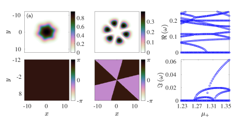
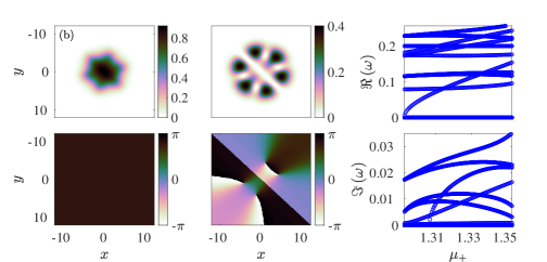
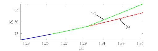
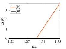
Figure 1: A bifurcation diagram of a bright-soliton-necklace state. In particular, the clustered panels (a) present the $|\phi_{-}|^{2}$ (top left) and $|\phi_{+}|^{2}$ (top middle), together with the respective phases (bottom left and middle panels therein). In addition, the associated spectra are presented where the real (top right) and imaginary (bottom right) parts of the relevant eigenfrequencies $\omega$ are depicted (for the real part of these eigenfrequencies only the lowest ones are shown). Similarly, the clustered panels (b) correspond to the bifurcated state of a stripe and two vortex dipoles in the second component emerging at $\mu_{+}\approx 1.293$. Bottom left and right panels correspond to the total number of atoms $N_{t}$ (left) and atom number difference $\Delta N_{t}$ (right) as functions of $\mu_{+}$ (see text for its definition). The vanishing of the latter is used to signal the bifurcation point. Recall that solid blue lines denote stability, while red and green dash-dotted ones exponential and oscillatory instability, respectively, in the bifurcation diagram here and in what follows.

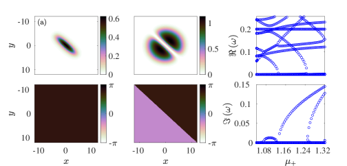
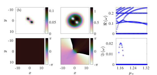
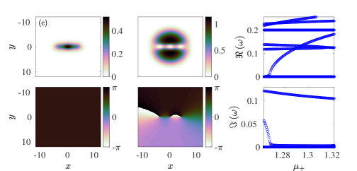
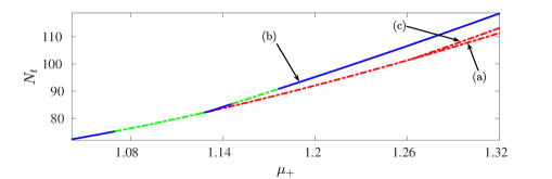
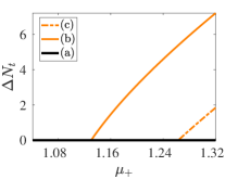
Figure 2: Same as Fig. 1 but for the dark-bright (DB) soliton stripe branch. All densities and respective phases presented in panels (a)-(c) are shown for values of $\mu_{+}$ of $\mu_{+}=1.32$. Note that bifurcations happen at $\mu_{+}\approx 1.13$ (b) and $\mu_{+}\approx 1.263$ (c), respectively. The emerging branches from the bifurcations of the DB stripe of the top panel are the VB dipole of the middle panel (b) and the VB soliton tripole of the lower panel (c).

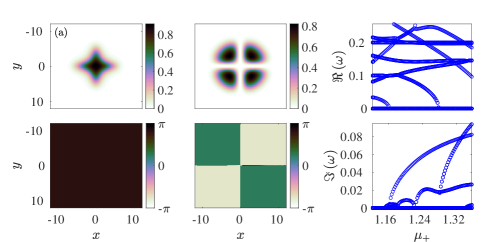
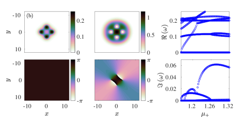
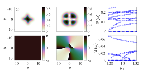
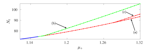
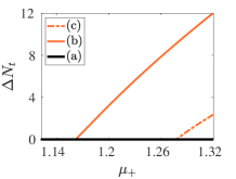
Figure 3: Same as Fig. 1 but for the crossed dark-bright (DB) soliton branch. Densities and phases shown in panels (a) and (b) correspond to a value of $\mu_{+}$ of $\mu_{+}=1.32$ whereas the ones presented in (c) correspond to $\mu_{+}=1.319$. Note that branch (b) emerges at $\mu_{+}\approx 1.162$ and branch (c) at $\mu_{+}\approx 1.279$. Branch (b) corresponds to a vortex-bright (VB) quadrupole, while in (c) a structure with additional vorticity at the center bifurcates from branch (a).

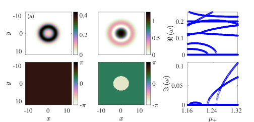
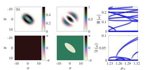
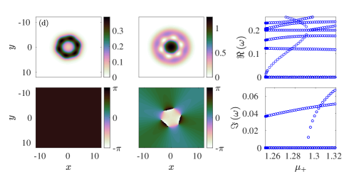
Figure 4: Same as Fig. 1 but for the dark-bright (DB) ring soliton branch. Densities and phases shown in panels (a), (b) and (c) correspond to a value of $\mu_{+}$ of $\mu_{+}=1.32$ whereas the one presented in (d) corresponds to $\mu_{+}=1.319$. Note that branch (b) emerges at $\mu_{+}\approx 1.222$, branch (c) at $\mu_{+}\approx 1.247$, and (d) at $\mu_{+}\approx 1.251$. The bifurcation diagram and total atom number difference (as a function of $\mu_{+}$) are shown in Fig. 5.

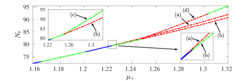
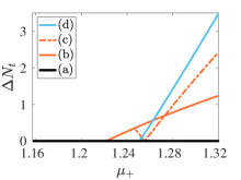
Figure 5: Continuation of Fig. 4. The left and right panels present the total number of atoms and total number of atoms difference both as functions of $\mu_{+}$. Notice the “spike” shown in the right panel as well as the fact that the $\Delta N_{t}$ of branches (b) and (c) from (a) become equal, i.e., equidistant from (a), at $\mu_{+}\approx 1.273$ corresponding to the intersection of their respective curves (see text for details).

According to the bifurcation diagram shown in the bottom left panel of Fig. 1, this bound state is stable from $\mu_{+}\approx 1.223$ (where the second component is formed, i.e., it is nontrivial) to $\mu_{+}\approx 1.256$. Given the instability of the soliton necklace in the single-component case of egc_16 , we infer that this stabilization is due to its coupling with the ground state of the first component. The state becomes oscillatorily unstable past the latter value of $\mu_{+}$. In addition, and as per the eigenvalue continuations in Fig. 1(a) a real eigenvalue –or equivalently an imaginary eigenfrequency– (see the top right panel therein) passes through the origin at $\mu_{+}\approx 1.293$, thus giving birth (through a pitchfork bifurcation yang_2012 ) to a new state having a stripe and two vortex dipoles in the second component one on each side of the stripe as is shown in Fig. 1(b) (see also the bottom right panel showcasing the atom difference of the bifurcated state from the parent branch). Past the bifurcation point ($\mu_{+}\approx 1.293$), the parent branch becomes exponentially unstable due to the relevant (purely) imaginary eigenfrequency, while the daughter branch bearing vorticity in this quadrupolar structure inherits the oscillatory instability that the parent branch featured before the bifurcation point (see the bifurcation diagram in the bottom left panel of Fig. 1).

Next, let us examine the results presented in Fig. 2. Specifically, Fig. 2(a) corresponds to the dark-bright (DB) soliton stripe branch. This state and its spectrum have been studied in pola_pra_2012 . More recently the theoretical analysis of such a dark-bright stripe and its transverse instability has also been considered in wenlong18 . According to the bifurcation diagram shown in the bottom left panel of the figure, this state is stable emanating from the linear limit (i.e., when the second component is almost absent) but it becomes oscillatory unstable for $\mu_{+}\approx[1.07,1.13]$. However, a sequence of pitchfork bifurcations happens at $\mu_{+}\approx 1.13$ and $\mu_{+}\approx 1.263$ giving birth to a vortex-bright (VB) soliton dipole branch of Fig. 2(b) which has been studied in pola_pra_2012 (see also wenlong18 for further analysis of this transverse instability) as well as the tripole branch (of alternating vortices) of Fig. 2(c) in the second component (see also the bottom right panel of the figure). This progression of first the dipole (of VB solitons), then the tripole, then an aligned quadrupole etc. is strongly reminiscent of the corresponding process of breakup of a stripe into multi-vortex states due to transverse instability in single-component BECs, as discussed, e.g., in middel10 . The dipole branch itself appears dynamically stable except for a narrow interval of oscillatory instability, once again analogous to the one-component case middel10 . On the other hand, the tripole branch is classified as exponentially unstable, inheriting the exponential instability of its parent DB stripe branch. While we are not aware of an experimental manifestation of states bearing multiple vortex-bright solitary waves, the ability to tune the experimentally realized DB solitons Becker2008 ; Middelkamp2011 ; Hamner2011 ; Yan2011 ; Hoefer2011 ; Yan2012 should, in principle, enable the realization of such observations, including, e.g., through the transverse instability of a dark-bright solitonic stripe. It is relevant to also mention that a single VB solitary wave has been previously realized experimentally in the work of brian_old .

A similar bifurcation pattern, i.e., a cascade of pitchfork bifurcations appears in Fig. 3. In particular, Fig. 3(a) corresponds to the crossed DB soliton stockhofe_jpb_2011 , i.e., a fundamental state in the first component and the $|1,1\rangle_{(\textrm{c})}\propto xye^{-\Omega(x^{2}+y^{2})/2}$ quadrupolar state in the second component as per its Cartesian representation at the linear limit. See, e.g., egc_16 for this representation; here, we remind the reader for completeness that Cartesian eigenstates of the linear limit can be denoted as

$$\ket{m,n}_{(\textrm{c})}\doteq\phi_{m,n}\sim H_{m}(\sqrt{\Omega}x)H_{n}(\sqrt{\Omega}y)e^{-\Omega r^{2}/2},$$ (17)

where $H_{m,n}$ stands for the Hermite polynomials with $m,n>0$, the quantum numbers of the harmonic oscillator. The associated energy of such a state (i.e., its eigenvalue) is $E_{m,n}\doteq(m+n+1)\Omega$ [cf. egc_16 ]. In the polar representation, we also have

$$\ket{k,l}_{(\textrm{p})}\doteq\phi_{k,l}=q_{k,l}(r)e^{il\theta}$$ (18)

with eigenvalues $E_{k,l}\doteq(1+|l|+2k)\Omega$. Here, $l$ and $k$ stand for the eigenvalue of the ($z$-component of the) angular momentum operator and the number of radial zeros of the corresponding eigenfunction $q_{k,l}$, respectively. The eigenfunction’s radial part can be denoted by

$$q_{k,l}\sim r^{l}L_{k}^{l}(\Omega r^{2})e^{-\Omega r^{2}/2},$$ (19)

where $L_{k}^{l}$ are the associated Laguerre polynomials. Interestingly once again, in the pattern of Fig. 3(a) note the astroid pattern of the first component induced by its phase immiscibility with the second component. The relevant state bifurcates from the linear limit (i.e., in the absence of the second component) and is dynamically stable for $\mu_{+}\approx[1.123,1.153]$. However, this branch becomes oscillatorily unstable for $\mu_{+}\approx[1.153,1.163]$ and past the value of $\mu_{+}\approx 1.163$, it becomes exponentially unstable (notice that this progression of instability is highlighted by the change of colors, i.e., from green to red in Fig. 3). In particular, the branch of Fig. 3(a) gives birth to the VB quadrupole cluster as was discussed in stockhofe_jpb_2011 at $\mu_{+}\approx 1.162$ shown in Fig. 3(b). The latter waveform is oscillatorily unstable over the interval of $\mu_{+}$ we consider herein. A subsequent pitchfork bifurcation happens later at $\mu_{+}\approx 1.279$ (see also the bottom right panel of the figure) giving birth to the state of Fig. 3(c). This state is exponentially unstable (due to the instability of its parent branch of Fig. 3(a)) and bears one vortex of charge 2 in the middle surrounded by another four vortices in the second component.

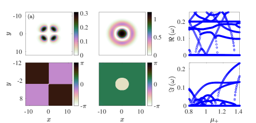
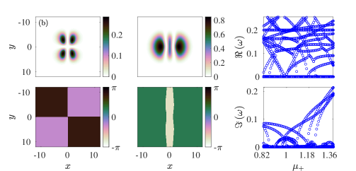
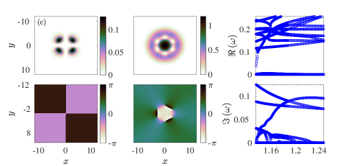
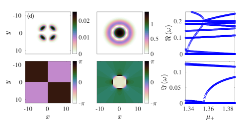
Figure 6: Same as Fig. 1 but for the quadrupolar ring-dark soliton (RDS) branch. The densities and respective profiles are shown for $\mu_{+}=1.2$ (a), $\mu_{+}=1.16$ (b), $\mu_{+}=1.2$ (c), and $\mu_{+}=1.377$ (d), respectively. The branches of (b), (c), and (d) emerge at values of $\mu_{+}$ of $\mu_{+}\approx 0.815$, $\mu_{+}\approx 1.135$ and $\mu_{+}\approx 1.336$, respectively.

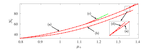
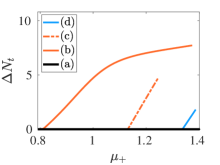
Figure 7: Continuation of Fig. 6. The left and right panels present the total number of atoms and total number of atoms difference both as functions of $\mu_{+}$. Note that the first component of the branch (b) vanishes past $\mu_{+}\approx 1.373$ as well as (c) does past $\mu_{+}\approx 1.244$ and (d) past $\mu_{+}=1.386$, respectively.

Subsequently, we focus on the DB ring soliton state of Fig. 4(a) and its bifurcations. This state (and in particular, with the first and second components reversed) has been identified and studied in stockhofe_jpb_2011 together with its stability. The state of Fig. 4(a) is generically unstable except for parametric intervals of stability $\mu_{+}\approx[1.157,1.164]$ and $\mu_{+}\approx[1.202,1.222]$. In particular, the DB ring soliton becomes oscillatory unstable past $\mu_{+}\approx 1.164$, then restabilizes itself at $\mu_{+}\approx 1.202$, and finally becomes exponentially unstable past $\mu_{+}\approx 1.222$. The first pitchfork bifurcation that takes place at $\mu_{+}\approx 1.222$ (a double imaginary eigenfrequency emanates from this collision) results in the emergence of the two DB soliton stripes shown in Fig. 4(b). This daughter branch inherits the stability of the parent branch and maintains its stability for a very short parametric interval (see the bottom right inset of the left panel of Fig. 5 showcasing the exchange of stability). Then, the two DB soliton stripes branch becomes oscillatorily unstable past $\mu_{+}\approx 1.223$, and then exponentially unstable past $\mu_{+}\approx 1.248$. It is worth pointing out about the additional co-existence of a smaller (in its imaginary part) oscillatorily unstable mode for $\mu_{+}\approx[1.2464,1.2784]$ being responsible for the emergence of a “bubble” as is shown in the imaginary part of the eigenfrequency spectrum. However, and slightly after the appearance of this “bubble”, a real eigenvalue crosses the origin at a value of $\mu_{+}$ of $\mu_{+}\approx 1.247$ giving birth to a secondary bifurcating branch shown in Fig. 4(c). This branch has been identified in stockhofe_jpb_2011 and is known as six vortex state with four of them being filled (i.e., VBs). This state inherits the oscillatory instability of the parent branch of Fig. 4(b) as well as gains further oscillatory unstable modes shortly after the bifurcation point $\mu_{+}\approx 1.247$ (see also the upper left inset of the left panel of Fig. 5). Finally, the parent branch of Fig. 4(a) undergoes one more bifurcation at $\mu_{+}\approx 1.251$ giving birth to the VB hexagon state stockhofe_jpb_2011 (again, the emerging unstable mode corresponds to a double imaginary eigenfrequency). This branch is shown in Fig. 4(d) and classified as exponentially unstable although past $\mu_{+}=1.303$, it also becomes oscillatorily unstable. All the above bifurcations are summarized in Fig. 5. Specifically, it should be noted that the branch of Fig. 4(c) emerging from the one of Fig. 4(b) and depicted with dashed-dotted orange line in the right panel of Fig. 5 has a “spike” at $\mu_{+}\approx 1.255$. The explanation of why this happens is offered in the following. Based on the definition of $\Delta N_{t}$ [cf. Eq. (16)], we measure the distance of $N_{t}$ [cf. Eq. (15)] of a bifurcating branch from a reference branch. Indeed, although the $N_{t}$ for branch (b) in Fig. 4 is smaller than the one for the reference branch (a) over the entire interval in $\mu_{+}$ considered therein, this difference appears positive in the right panel of Fig. 5, based on the definition of the relevant diagnostic. Furthermore, the “spike” of the curve therein corresponding to the difference of $N_{t}$ between branches (c) and (a) happens because the $N_{t}$ of the former branch (as this emerges from branch (b)) is smaller than the $N_{t}$ of branch (a) (and larger than the $N_{t}$ of branch (b)) until its curve (as a function of $\mu_{+}$), intersects the corresponding one of branch (a) at $\mu_{+}\approx 1.255$. Then, and past that value, the $N_{t}$ of branch (c) is larger than the one of branch (a).

Hereafter, the configurations become more complex. The quadrupolar type solution in the first component described as $|1,1\rangle_{(\textrm{c})}$ in its Cartesian classification trapping a ring-dark soliton (RDS) in the second component is shown in Fig. 6(a). This branch emerges, i.e., bearing a non-trivial solution in its second component at $\mu_{+}\approx 0.791$ and is classified as exponentially unstable over the parametric interval of $\mu_{+}\approx[0.791,1.4]$. Similarly, the branch of Fig. 6(a) undergoes a pitchfork bifurcation at $\mu_{+}\approx 0.815$ giving birth to the daughter branch of Fig. 6(b). This branch bears a two-dark soliton stripes waveform (or $|2,0\rangle_{(\textrm{c})}$ as per its Cartesian classification) in the second component whose total number of atoms is less than its parent branch (see the left panel of Fig. 7). In addition, this state is classified as exponentially unstable throughout its interval of existence where the first component vanishes eventually at $\mu_{+}\approx 1.373$. A subsequent pitchfork bifurcation of the parent branch [cf. Fig 6(a)] occurs at $\mu_{+}\approx 1.135$ where the branch of Fig. 6(c) bearing a hexapolar mode in the second component egc_16 is born. This branch, i.e., the quadrupolar-vortex-hexagon branch is classified as exponentially unstable over $\mu_{+}\approx[1.135,1.187]$ and past the value of $\mu_{+}\approx 1.187$ possesses a dominant oscillatory unstable mode (see the left panel of Fig. 7), thus mimicking the spectrum in the single-component case egc_16 . Finally, and as the value of $\mu_{+}$ increases, the parent branch of Fig. 6(a) undergoes one more pitchfork bifurcation giving birth to the quadrupolar vortex-octagons state of Fig. 6(d). Such a pattern, i.e., the subsequent bifurcations of the RDS state was briefly mentioned in the one-component case egc_16 . In our case, the branch of Fig. 6(d) has a narrow interval of existence of $\mu_{+}\approx[1.336,1.386]$ in which it is classified as exponentially unstable according to our spectral stability analysis (see the left panel of Fig. 7). Finally, it should be noted that the total number of atoms of branch (b) is less than the one of the parent branch of (a). Similarly to the case of the branches of Figs. 4(a) and 4(b), this difference is shown in the right panel of Fig. 7 and depicted with a solid orange line therein.

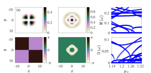
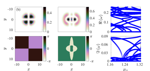
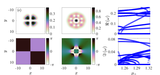
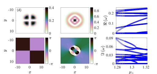
Figure 8: Same as Fig. 1 but for the quadrupolar–two dark rings branch. The branches (a)-(d) are presented for a value of $\mu_{+}$ of $\mu_{+}=1.32$. The branch of panel (a) undergoes a cascade of pitchfork bifurcations occurring at $\mu_{+}\approx 1.16$, $\mu_{+}\approx 1.242$ and $\mu_{+}\approx 1.277$, thus giving birth to the branches of panels (b), (c) and (d), respectively.

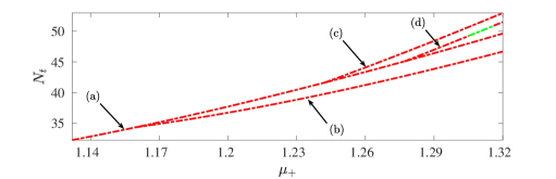
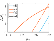
Figure 9: Continuation of Fig. 8. The left and right panels present the total number of atoms and total number of atoms difference both as functions of $\mu_{+}$. According to the left panel, the $N_{t}$ of branch (b) is less than the one of its parent branch (a). Similarly to Fig. 5 the $\Delta N_{t}$ of branches (b) and (c) from (a) become equal, i.e., equidistant from (a), at $\mu_{+}\approx 1.3075$ corresponding to the intersection of their respective curves (see text for details).

Next, we turn to the case of Fig. 8. In particular, Fig. 8(a) presents a quadrupolar waveform in the first component which, in turn, is coupled to a state bearing two dark rings in the second component. This state has lost its radial symmetry, though, due to the immiscibility (and the effects of nonlinear coupling) between the two components. This bound mode is exponentially unstable over the parametric interval in $\mu_{+}$ considered herein (see the left panel of Fig. 9). However, there is again a cascade of pitchfork bifurcations, the first of which occurs at $\mu_{+}\approx 1.16$ as is also highlighted in the right panel of Fig. 9. In particular, the first bifurcating branch is shown in Fig. 8(b) where the solution in the second component can be thought of as a symmetry-broken (between the axes) variant of panel (a) that can be represented as a $|4,0\rangle_{(\textrm{c})}+|2,2\rangle_{(\textrm{c})}$ Cartesian state at the linear limit. In the present two-component case, the branch of Fig. 8(b) is exponentially unstable as well (see the left panel of Fig. 9). The next pitchfork bifurcation occurs at $\mu_{+}\approx 1.242$ where Fig. 8(a) gives birth to the bound mode shown in Fig. 8(c) with the second component featuring an intriguing combination of a ring and a vortex necklace. Although this solution has been identified as oscillatorily unstable in egc_16 in the single-component NLS, the daughter branch shown in Fig. 8(c) is classified to be exponentially unstable (see the left panel of Fig. 9). It is interesting to highlight here that although in some cases (such as in Fig. 1(a) as we saw before) the presence of a second component plays a stabilizing role, in others such as the one of Fig. 8(c), it adds further unstable eigendirections to a particular waveform. Finally, the parent branch of Fig. 8(a) undergoes one further pitchfork bifurcation at $\mu_{+}\approx 1.277$ giving birth to the daughter branch of Fig. 8(d). This branch forms four vortices in its inner ring and is generally exponentially unstable (over the interval we considered herein) except for a narrow interval of $\mu_{+}\approx[1.305,1.316]$ where the dominant instability appears to be an oscillatory one (co-existing with a number of weaker exponentially unstable eigendirections). Similarly as in Figs. 5 and 7, the left panel of Fig. 9 suggests that although the total number of atoms $N_{t}$ of the bifurcating branch of Fig. 8(b) is less than the one of its parent branch [cf. Fig. 8(a)], the respective total-number-of-atoms difference between those two branches is positive as is shown in the right panel of Fig. 9 per the definition of Eq. (16).

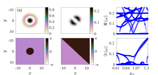
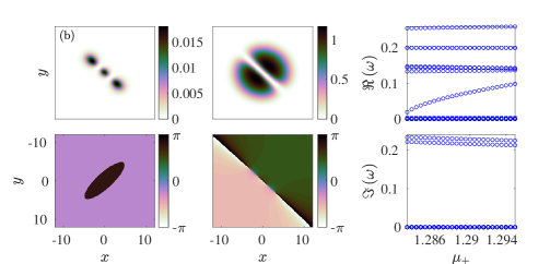
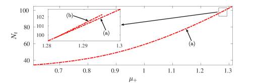
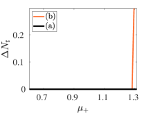
Figure 10: Same as Fig. 1 but for the ring-dark-soliton-dipolar (RDS-dipolar) branch. The densities and associated phases are shown for values of $\mu_{+}$ of $\mu_{+}=0.7$ (a) and $\mu_{+}=1.29$ (b), respectively in the first and second rows. Note that the branch of panel (b) emerges at $\mu_{+}\approx 1.282$. The bottom left and right panels present the total number of atoms and total-number-of-atoms difference both as functions of $\mu_{+}$.

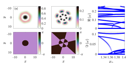
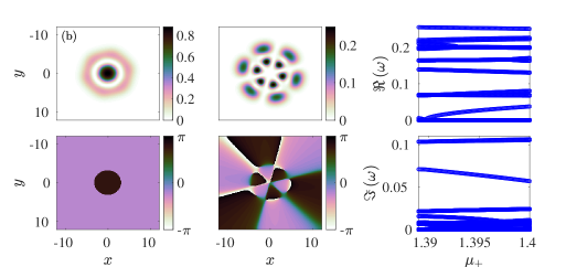
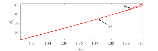
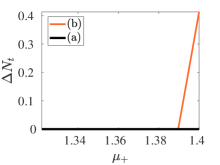
Figure 11: Same as Fig. 1 but for the hexagonal type RDS-necklace branch. Similarly, the densities and associated phases are shown for a value of $\mu_{+}$ of $\mu_{+}=1.4$ for both branches. The branch (b) emerges at $\mu_{+}\approx 1.39$ via a pitchfork bifurcation. Again, the bottom left and right panels present the total number of atoms and total-number-of-atoms difference both as functions of $\mu_{+}$.

The state of Fig. 10(a) involves a symmetry-broken state where the first component features an elliptical type of a RDS, while the second component represents a dipolar ($|1,0\rangle_{(\textrm{c})}$ in the notation of the Cartesian Hermite eigenstates) structure bearing a $\pi$ phase shift between the two matter wave blobs. This branch is highly unstable and in fact, classified as exponentially unstable over $\mu_{+}\approx[0.607,1.313]$ as is shown in the bottom left panel of Fig. 10 where the first component vanishes past $\mu_{+}\approx 1.313$. However, and close to the limit in $\mu_{+}$ where the first component vanishes, this branch undergoes a similar symmetry-breaking bifurcation as in the previous cases in this work giving birth to the branch of Fig. 10(b) (see also the bottom right panel of Fig. 10). This daughter branch involves a series of density blobs in the first component centered along the nodal line of the second component. The latter features a vortex quadrupole (this is hard to discern at the level of the density but more transparent at the level of the phase of this component) which is exponentially unstable as is also shown in the inset in the bottom left panel of Fig. 10; its interval of existence over $\mu_{+}$ is rather narrow (the first component is non-vanishing for $\mu_{+}\approx[1.282,1.295]$). It should be noted in passing that the branch of Fig. 10(b) is a typical example among the pitchfork bifurcations that are expected to emerge from Fig. 10(a) at values of $\mu_{+}\approx 0.67,0.9$ and $\mu_{+}\approx 0.99$ where the first two will correspond to reverse pitchfork bifurcations (see, Figs. 12(c) and 13(g) next for an example of such a bifurcation).

On the other hand, and as per the branch of Fig. 11(a), the first component features similarly a RDS whereas the second component involves a hexapolar double soliton necklace. The latter state (which also deforms the RDS into a pattern with hexagonal symmetry due to the nonlinear interactions) was identified in the previous work of egc_16 in the single-component case and classified as exponentially unstable. In the present two-component case, the bound mode of Fig. 11(a) is exponentially unstable over the reported interval of $\mu_{+}\approx[1.3219,1.4]$ (see the bottom left panel of Fig. 11). The double solitonic necklace emerges at $\mu_{+}\approx 1.3219$; Subsequently, a real eigenvalue passes through the origin at $\mu_{+}\approx 1.39$ giving birth (via a pitchfork bifurcation) to the branch of Fig. 11(b) (see the bottom right panel of Fig. 11). This branch, in turn, features a vortex necklace (notice the modification in the relevant phase profile from the purely real parent branch of Fig. 11(a)) and is classified as exponentially unstable over the reported interval of $\mu_{+}\approx[1.39,1.4]$ as is shown in the bottom left panel of Fig. 11.

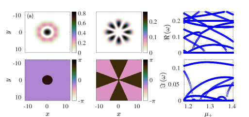
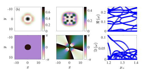
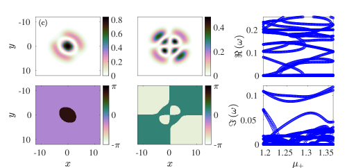
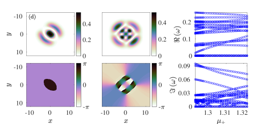
Figure 12: Same as Fig. 1 but for the RDS-necklace branch. All densities and phases are shown for a value of $\mu_{+}=1.3$ except of (d) corresponding to $\mu_{+}\approx 1.32$. The branch of panel (a) emerges at $\mu_{+}\approx 1.177$. The branches (b) and (c) emanate from (a) at $\mu_{+}\approx 1.19$ and $\mu_{+}\approx 1.192$, respectively. The branch (c) merges with the branch of Fig. 13(g) at $\mu_{+}\approx 1.362$ (see text for details). Finally, the branch of panel (d) emerges at $\mu_{+}\approx 1.291$ from (c).

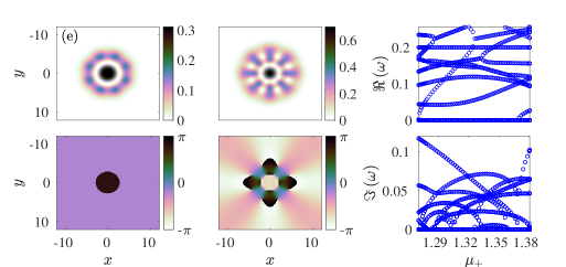
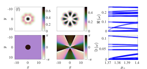
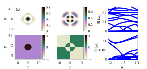
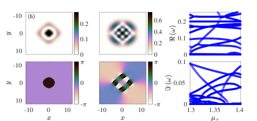
Figure 13: Continuation of Fig. 12. Densities and phases are presented for values of $\mu_{+}$ of $\mu_{+}=1.32$ (e), $\mu_{+}=1.4$ (f), $\mu_{+}=1.4$ (g), and $\mu_{+}=1.4$ (h), respectively. The branch of panel (e) emerges at $\mu_{+}\approx 1.27$ and vanishes at $\mu_{+}\approx 1.381$ whereas the branch of (f) emerges at $\mu_{+}\approx 1.37$ and is shown up to $\mu_{+}=1.4$. Finally, the branch of panel (g) emerges at $\mu_{+}\approx 1.1896$ (linear limit) giving birth to branch (h) at $\mu_{+}\approx 1.296$.

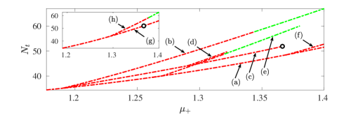
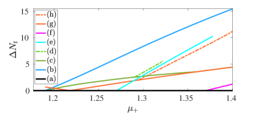
Figure 14: Continuation of Fig. 12 and also 13. The total number of atoms and total number of atoms difference are shown in the top and bottom panels, respectively as functions of $\mu_{+}$. The black open circles in the top panel are explained in the text.

We turn now our focus on the branches presented in Figs. 12, 13 and 14. Specifically, the branch of Fig. 12(a) involves a RDS-necklace state whose first component is a RDS of octagonal type and bears small “blobs” in its density. These blobs are complementary (due to inter-component repulsion) to the ones of the solitonic necklace of the second component. This bound mode emerges from the linear limit at $\mu_{+}\approx 1.177$ and is classified (according to our spectral stability analysis) as exponentially unstable over $\mu_{+}=[1.177,1.4]$ (see also the top panel of Fig. 14). In addition, this branch gives birth to the structures of Fig. 12(b) and 12(c), respectively through pitchfork bifurcations. In particular, the state of Fig. 12(b) emerges at $\mu_{+}\approx 1.19$ and features a vortex necklace in the second component (see also the bottom panel of Fig. 14). It can be discerned from the second component of Fig. 12(b) that the blobs of the necklace of its parent branch [cf. Fig 12(a)] re-arrange themselves due to the emergence of vorticity therein. Based on our spectral stability analysis, this state is classified as exponentially unstable over $\mu_{+}\approx[1.19,1.344]$ and oscillatorily unstable past $\mu_{+}\approx 1.344$ (see the top panel of Fig. 14). Furthermore, the soliton necklace in the second component of the branch of Fig. 12(a) undergoes a density re-arrangement in its blobs at $\mu_{+}\approx 1.192$ resulting in the bound state of Fig. 12(c) whose first component is morphed into an elliptical RDS state and is classified as exponentially unstable over $\mu_{+}\approx[1.192,1.362]$. Although we do not exhaustively discuss secondary bifurcations in this work, we report the emergence of the branch depicted in Fig. 12(d) which emanates via a pitchfork bifurcation of its parent branch [cf. Fig. 12(c)] at $\mu_{+}\approx 1.291$. This branch is exponentially unstable over the interval of $\mu_{+}\approx[1.291,1.322]$ (results past $\mu_{+}\approx 1.322$ are not shown) as is depicted in the top panel of Fig. 14. Subsequently, the branch of Fig. 12(a) undergoes two further pitchfork bifurcations at $\mu_{+}\approx 1.27$ and $\mu_{+}\approx 1.37$, respectively. The first bifurcating state is shown in Fig. 13(e) which involves a vortex necklace of octagonal shape in the second component. The latter state was identified in the single-component NLS equation in egc_16 (and references therein) as a combination of a double ring configuration and a necklace. According to our stability analysis results shown in the top panel of Fig. 14, this branch is exponentially unstable for $\mu_{+}\approx[1.27,1.32]$ and oscillatorily unstable for $\mu_{+}\approx[1.32,1.381]$ (note that the second component vanishes past $\mu_{+}\approx 1.381$). At the same time, the branch of Fig. 13(f) features another vortex necklace in its second component. This branch is classified as exponentially unstable over $\mu_{+}\approx[1.37,1.4]$ (results are not shown past $\mu_{+}=1.4$). Surprisingly, the branch of Fig. 12(c) at $\mu_{+}\approx 1.362$ merges with the branch of Fig. 13(g) (see also the black open circles in the bifurcation diagram in the top panel of Fig. 14). This merging of 12(c) with 13(g) is a canonical example of a reverse pitchfork bifurcation where the branch of Fig. 13(g) is the parent branch. This branch is classified as exponentially unstable. However, as $\mu_{+}$ increases and at $\mu_{+}\approx 1.296$, the branch of Fig. 13(g) undergoes a pitchfork bifurcation giving birth to the state of Fig. 13(h) bearing a cluster of twelve vortices in the outer ring and four charge-one vortices in arranged in a cross shape. Notice that adjacent vortices in the pattern bear opposite charges lending the overall pattern a vanishing net vorticity. This branch is classified as exponentially unstable except for a narrow interval of $\mu_{+}\approx[1.377,1.4]$ over which it appears (dominantly to be) oscillatorily unstable as is shown in the top panel of Fig. 14 (this branch is not shown for values of $\mu_{+}$ past $\mu_{+}\approx 1.4$). Our results on all the above branches are summarized in the top and bottom panels of Fig. 14 highlighting the dominant instability and bifurcations, respectively.

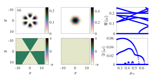
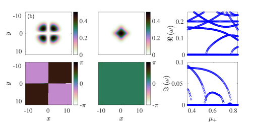
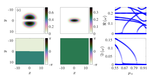
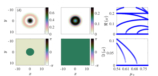
Figure 15: Branches of solutions that are reversed versions of ones discussed previously in this work. Densities and phases as well as associated spectra are shown for $\mu_{+}=0.52$ (a) (reversed version of Fig. 1(a)), $\mu_{+}=0.6$ (b) (reversed version of Fig. 3(a)), $\mu_{+}=0.68$ (c) (reversed version of Fig. 2(a)), and $\mu_{+}=0.65$ (d) (reversed version of Fig. 4(a)), respectively.

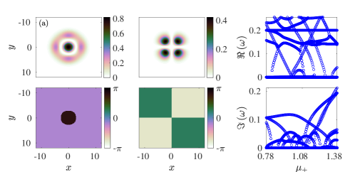
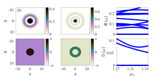
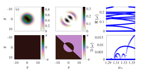
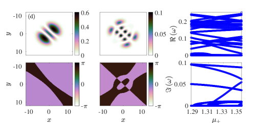
Figure 16: Same as Fig. 15. Note that panel (a) depicted for $\mu_{+}=0.95$ is a reversed version of Fig. 6(a). The branches of panels (b)-(d) are all presented for a value of $\mu_{+}$ of $\mu_{+}=1.32$ at which the first component does not become the trivial solution.

Finally, we discuss about the branches presented in Figs. 15 and 16 that the DCM identified. In Figs. 15(a)-(d) and Fig. 16(a), we observe a series of states that are variants of states that we have already encountered, albeit now in reverse i.e., with the second component playing the role of the first one and vice versa. Recall that in the case of the equal $g_{ij}$ (the so-called Manakov model integrable in one-dimension abl3 ), these states would be interchangeable, however the weak asymmetry (and corresponding immiscibility) distinguishes between these states and the earlier ones. Indeed, Fig. 15(a) provides a reversed analogue of Fig. 1(a) whereas the branch of Fig. 15(b) can be similarly connected to Fig. 3(a). These branches involve multipoles (a hexapole and a quadrupole) coupled to a fundamental state. The branch of Fig. 15(c) presents a DB solitonic stripe, analogous to that of Fig. 2(a). Also, the branch of Fig. 15(d) is tantamount to Fig. 4(a), namely the ring dark-bright soliton, whereas the branch of Fig. 16(a) is strongly reminiscent of the branch of Fig. 6(a) involving a RDS and the $|1,1\rangle_{(\textrm{c})}$ (in its Cartesian classification) state. In view of these similarities and the slight asymmetries of the $g_{ij}$, the precise instability details of the states of Fig. 15(a)-(d) and Fig. 16(a) are somewhat different, yet qualitatively similar to the examples that we have already studied above. It should be noted that we performed the continuation of all the above branches over $\mu_{+}$ and stopped when one of the components was found to be below numerical precision, i.e., when effectively the states become single component waveforms with the other component being trivial. Indicatively, the intervals of existence (and stability) of the states shown in Fig. 15 are $\mu_{+}\approx[0.2474,0.6769]$ (a) (stable over $\mu_{+}\approx[0.634,0.6769]$), $\mu_{+}\approx[0.542,0.9275]$ (b) (stable over $\mu_{+}\approx[0.84,0.9275]$), $\mu_{+}\approx[0.35,0.8335]$ (c) (stable over $\mu_{+}\approx[0.775,0.8335]$), $\mu_{+}\approx[0.531,0.778]$ (d) (stable over $\mu_{+}\approx[0.6925,0.778]$), as well as the one of Fig. 16(a) is $\mu_{+}\approx[0.764,1.385]$ (and is exponentially unstable over the relevant range in $\mu_{+}$).

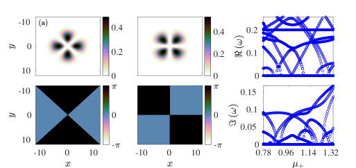
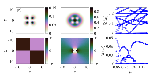
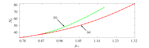
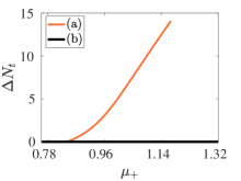
Figure 17: Same as Fig. 1 but for the rotated dipolar branch. Densities and phases are shown in panels (a) and (b) for values of $\mu_{+}$ of $\mu_{+}=1$ and $\mu_{+}=1.1$, respectively. The bound state involving the vortex quadrupole in the second component of panel (b) emerges at $\mu_{+}\approx 0.845$. Similarly, the bottom left and right panels present the total number of atoms and number-of-atoms difference, respectively.

As we advance to panels (b)-(d) of Fig. 16, we encounter higher excited state combinations. For instance, in Fig. 16(b), a double RDS in the second component is coupled to a single RDS in the first component (this bound state emerges at $\mu_{+}\approx 1.269$). It is important to recall, in line with the discussion of egc_16 , that these ring states are eigenstates (with $l=0$ azimuthal index) of the associated Laguerre eigenmodes of the two-dimensional system. In particular, these are modes with $k=2$ in the second component and $k=1$ in the first component. Subsequently, in Fig. 16(c), a fundamental state in the first component is coupled with the multipole $|2,1\rangle_{(\textrm{c})}+|0,3\rangle_{(\textrm{c})}$ in the notation of the Cartesian Hermite eigenstates resulting in a bound state emerging at $\mu_{+}\approx 1.283$ as a stable branch until $\mu_{+}\approx 1.302$. The branch of Fig. 16(d) emerges at $\mu_{+}\approx 1.286$ and features a higher order example of a Cartesian excited state. Here, a $|4,1\rangle_{(\textrm{c})}$ state in the second component is coupled to a $|2,0\rangle_{(\textrm{c})}$ one in the first component. This bound state features a multiplicity of exponentially unstable modes, in addition to a number of oscillatory instabilities in suitable parametric ranges. Finally, it should be noted that all the above states with the exception of that of Fig. 16(c) are very highly unstable, as can be seen from the right panels of Fig. 16. Yet, it is relevant to comment that some of these highly excited states like the one depicted in Fig. 16(c) may feature intervals of spectral stability and the highly accurate numerical techniques used herein can identify these states and their corresponding stability intervals.

III.1 Further linear modes and DCM

The DCM was initialized at $\mu_{+}=0.492$, using as initial guess for Newton’s method a Gaussian in each component; this converged to the solution shown in Fig 15(c). At each subsequent continuation step, the solutions at the previous step were used as initial guesses. This strategy does not exploit our analytical knowledge of the problem, specifically our knowledge of eigenstates in the linear limit. Despite this disadvantage, the DCM identified a large number of solutions.

However, it did not identify all known branches (e.g. ones that are present in the single-component NLS equation). This motivated an effort to identify further ones (in addition to the states obtained via DCM) using the physical understanding of the system and the linear limits. That is to say, we utilized linear eigenstates in each of the components in either a Cartesian [cf. Eq. (17)] or a polar [cf. Eqs. (18) and (19)] form and continued relevant combinations for suitable choices of $\mu_{+}$ and $\mu_{-}$ to the nonlinear regime, i.e., for non-vanishing values of $N_{+}$ and $N_{-}$. To this end, we briefly discuss a few examples (among several others) shown in Figs. 17 and 18 that could be used in addition to the results of the DCM method. We note in passing that we have found numerous additional branches to the ones reported here (stemming from the linear limit). However, we refrain from discussing all of them here to avoid cluttering the manuscript with additional figures.

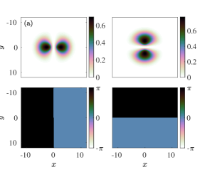
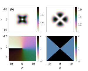
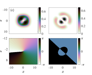
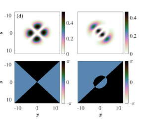
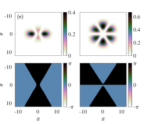
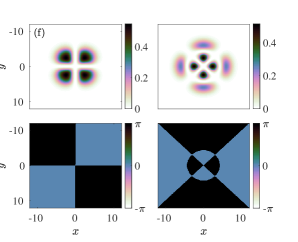
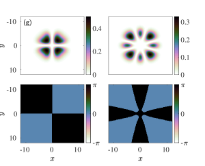
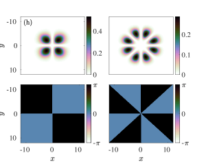
Figure 18: Other branches of solutions identified via continuation from the linear limit (see text for details). Densities and phases are shown for $\mu_{+}=1$ (a) and $\mu_{+}=1.21$ (b), $\mu_{+}=1.26$ (c), $\mu_{+}=1.1$ (d), $\mu_{+}=1.232$ (e), $\mu_{+}=1.27$ (f), $\mu_{+}=1.3$ (g) and $\mu_{+}=1.3$ (h), respectively.

We begin our discussion with the quadrupolar complex of Fig. 17(a). In particular, one can envision the $|1,1\rangle_{(\textrm{c})}$ state in the one component co-existing with its rotated version in the second component (due to the mutual repulsion between components and their immiscibility) as is shown in the figure. This bound state emerges at $\mu_{+}\approx 0.76$ and is classified as exponentially unstable over $\mu_{+}\approx[0.76,1.32]$ (we did not perform the continuation past $\mu_{+}=1.32$). From its associated spectrum, a cascade of pitchfork bifurcations can be discerned, the first of which takes place at $\mu_{+}\approx 0.845$. The branch that emerges out of this mechanism is presented in Fig. 17(b) featuring a vortex quadrupole in the second component (the latter state was identified in egc_16 for the single-component NLS equation). The emerging branch amounts to a vortex bright quadrupole. It is exponentially unstable for $\mu_{+}\approx[0.845,0.89]$ and then oscillatorily unstable until $\mu_{+}\approx 1.172$ where the first component vanishes, thus reducing to the single-component case. The single component vortex quadrupole features an interval of oscillatory instability but is otherwise dynamically stable; see e.g., egc_16 and references therein.

To offer an anthology of possible states that we have been able to identify on the basis of continuation from the linear limit, we refer the reader to Fig. 18. These (together with the branches shown in Fig. 17) constitute examples of nonlinear eigenstates of the problem that we have continued from their respective linear limit up to $\mu_{+}=1.32$. However, it is important to highlight that these states were not obtained via the DCM.

Although typical examples of the relevant solutions are shown, we do not present their associated spectra: we simply present them as representative examples of the richness of additional available nonlinear patterns that a physical understanding of relevant limits can enable us to access. Nevertheless, we briefly comment on intervals of stability (when applicable) and instability of these waveforms. Similarly as in Fig. 17(a), one can construct a dipole state (in the form of $|1,0\rangle_{(\textrm{c})}$ in the first component) featuring its rotated version in the second component as is shown in Fig. 18(a). This state emerges at $\mu_{+}\approx 0.681$ and is generally exponentially unstable except for the interval of $\mu_{+}\approx[0.9262,1.05]$ in which it appears to be oscillatorilly unstable. The bound state mode of Fig. 18(b) features a single charge vortex in the first component and the $|1,1\rangle_{(\textrm{c})}$ in the second component. This complex is classified as stable for $\mu_{+}\approx[1.095,1.097]$ (as it emerges from the linear limit in the second component) but then becomes oscillatorily unstable except of $\mu_{+}\approx[1.195,1.214]$. Furthermore, the solution of Fig. 18(c) involves a deformed vortex in the first component and a $\Phi$ mode in the second component. This state bifurcates from the linear limit at $\mu_{+}\approx 1.191$ and is classified as stable for $\mu_{+}\approx[1.191,1.198]$. For larger values of $\mu_{+}$ it becomes oscillatorily unstable up to $\mu_{+}\approx 1.212$ where it starts featuring a dominant exponentially unstable mode. Next, all solutions of panels (d)-(h) of Fig. 18 involve the $|1,1\rangle_{(\textrm{c})}$ state in the first component and the states in the second component bifurcate at $\mu_{+}\approx 0.9462$, $\mu_{+}\approx 1.089$, $\mu_{+}\approx 1.098$, $\mu_{+}\approx 1.22$, and $\mu_{+}\approx 1.224$, respectively. In particular, the solution of Fig. 18(d) features a $|3,0\rangle_{(\textrm{c})}$ in the second component whereas the $|1,1\rangle_{(\textrm{c})}$ in Fig. 18(e) traps a soliton necklace as this is the case with the second component of Fig. 18(g) and (h). In Fig. 18(f), the solution that is trapped in the second component can be approximated in their linear limit by a linear combination of Cartesian eigenstates egc_16 (see also the second component of Fig. 13(g)). The solutions of Figs. (d)-(h) are all classified as exponentially unstable.

IV Concluding remarks and future challenges

In the present work, we have shed some light on the wealth and complexity of the pattern formation that arises in the context of two-component atomic Bose-Einstein condensates, revealed by a state-of-the-art numerical technique. Naturally, some of the states that we explored have been previously considered in earlier studies such as pola_pra_2012 ; stockhofe_jpb_2011 ; wenlong18 (among others) or represent two-component extensions of single-component ones. However, several of the states found have not previously been discussed in the literature, to the best of our knowledge. In addition to identifying these states, we explored their bifurcation structure and gave a systematic mapping of the parametric regions (as a function of the chemical potential of the second component) where the states were potentially stable, exponentially or oscillatorily unstable.

Naturally, there are numerous directions of further work to pursue. A clear starting point is that of seeking a way for obtaining a complete “cartography” of the possible nonlinear states of the model. We saw that the DCM offers a rich repository of such states. Similarly, we argued that the linear limit and its theoretical understanding provides plenty more. Additionally bifurcation events from the existing states lead to even more. Yet, no toolbox at the moment appears to allow a systematic classification of the full span of the highly nonlinear states in this system. A summary of the current techniques and their advantages and disadvantages will be a useful tool for further efforts. Moreover, to date we have focused on two-dimensional states, but it is particularly relevant to study three-dimensional configurations in both single but also multi-component settings. Another direction where recently solitonic pattern formation has been pursued is that of spinor BECs; see e.g. Bersano2018 for a recent example of solitonic states. It is thus of particular interest to examine how spin-dependent interactions especially may modify the states stemming from a three-component analogue of the Manakov model. The three-component Manakov setting in this case represents effectively the spin-independent interaction, while the spin-dependent one is weak, but rather complex in that it involves nontrivial phase dynamics between the components kawueda . These are extensions worth pursuing from a physical perspective.

From the numerical analysis/algorithmic perspective, we should comment that further extensions to the DCM that we are currently exploring would enable it to discover more solutions. First, using the linear eigenstates as initial guesses at the appropriate value of $\mu_{+}$ would give it more branches to track, and therefore more initial guesses to use at each continuation step. Second, branch switching algorithms (as implemented in, e.g., AUTO doedel1986 ) could be applied to branches identified via deflation, combining their advantages. Third, deflation can be combined with nested iteration to greatly enhance its robustness adler2017 . Fourth, the use of more robust nonlinear solvers (improved line searches or trust region techniques) would make the solution of deflated problems more successful on average. Together, these extensions could substantially enhance the ability of deflation to reveal previously unknown solutions to nonlinear partial differential equations and, thus, represent a direction worth pursuing in its own right.

Appendix A State-of-the-art eigenvalue computations using FEAST

In this appendix we briefly give more details of the eigenvalue computations associated with Eq. (12). Upon convergence of Newton’s method (with $10^{-9}$ relative and absolute tolerances, respectively), the stability matrix $A$ of Eq. (12) is computed. For the finite difference discretization employed, the matrix $A$ is a $357,604\times 357,604$ sparse matrix with $2,856,048$ non-zero elements. To compute its eigenvalues, we initially used MATLAB’s eigs command which employs a Krylov-Schur method mathworks_eigs to compute a subset of the eigenvalues. Although MATLAB did not raise any warnings during the computation (i.e., flag=0), in some of the cases the obtained spectrum contained spurious eigenvalues. This finding was further investigated by calculating

$$\frac{\underset{1\leq i\leq n_{\textrm{max}}}{\max}\left\|A\textbf{W}_{\textrm{R}}^{(i)}-\rho_{i}\textbf{W}_{\textrm{R}}^{(i)}\right\|_{\ell_{1}}}{\left\|A\right\|_{\ell_{1}}},$$ (20)

where $n_{\textrm{max}}$ is the number of eigenpairs computed, and $\textbf{W}_{\textrm{R}}^{(i)}$ is the $i$th right eigenvector associated with the eigenvalue $\rho_{i}$. For instance, Eq. (20) evaluated for the solution of the branch shown in Fig. 2(c) and for $\mu_{+}=1.32$ gives $\approx 2.21$ for $100$ eigenpairs. One possible explanation about why this happens is given next pavel . MATLAB’s eigs computes first the LU decomposition (with full pivoting and scaling) of the matrix $A$, which is performed very accurately. However, the matrix $A$ itself is ill-conditioned (as we will see subsequently) and any slight change in subspace vectors in the Krylov-Schur algorithm will lead to a large change in resulting eigenvectors saad . As a consequence, all the accuracy is lost by using eigs without any warning raised.

To further investigate this issue, we used the Multiprecision Computing Toolbox “Advanpix” advanpix which implements an extended precision version of eigs function called mpeigs. We performed the eigenvalue computation of the branch shown in Fig. 2(c) with $34$ digits (over $121$ distinct values of $\mu_{+}$) which took approximately 3 months of computing time on an Intel(R) Xeon(R) CPU E5-2670 0 @ 2.60GHz processor with 64GB of RAM. The respective results are shown with red stars in the left and right panels of Fig. 19 corresponding to the real and imaginary parts of $\omega$, respectively. We further checked Eq. (20) for this computation and for, e.g., $\mu_{+}=1.32$ we found that the residual of Eq. (20) for $100$ eigenpairs $\left(\rho,\textbf{W}_{\textrm{R}}\right)$ was $\approx 1.57\times 10^{-18}$. This computation clearly suggests that extended precision is capable of diminishing any small perturbations in subspace vectors in the Krylov-Schur algorithm.

However, a new algorithm (motivated by contour integration and density-matrix representation in quantum mechanics) for solving eigenvalue problems known as FEAST was introduced in eric_1 (see also tang_eric for details). FEAST itself combines accuracy, efficiency and robustness while exhibiting natural parallelism at multiple levels. Recently, the algorithm was generalized and applied to non-Hermitian matrices kestyn_eric_tang (and references therein). In our present work, we used FEAST extensively to calculate the spectra of all branches shown with $10^{-8}$ relative tolerance (on the residuals) as the stopping criterion (e.g., for the branch of Fig. 2(c) and for $\mu_{+}=1.32$, Eq. (20) gives $\approx 1.39\times 10^{-8}$ for $100$ eigenpairs). It should be noted that FEAST converges quite quickly ($3$ to $5$ iterations were required in most of the cases we studied), thus providing us with a robust tool for solving large eigenvalue problems. Its execution time varies depending on the number of eigenvalues inside a prescribed contour. Indicatively, the computation of the eigenvalues of the branch of Fig. 2(c) took approximately $5$ hours.

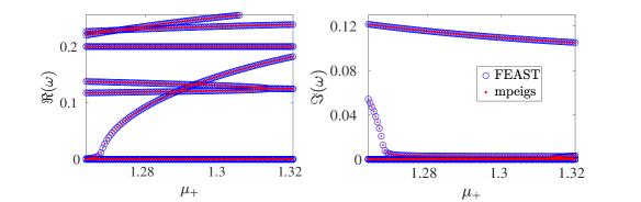
Figure 19: The eigenfrequencies of Eq. (12) obtained by using the FEAST eigenvalue solver and mpeigs— are shown with blue open circles and red stars for comparison.

To further demonstrate the robustness of the FEAST algorithm, we calculate the condition number of a simple eigenvalue $\rho$ saad defined by

$$\kappa\left(\rho\right)=\frac{\left\|\textbf{W}_{\textrm{R}}\right\|_{\ell_{2}}\left\|\textbf{W}_{\textrm{L}}\right\|_{\ell_{2}}}{|\left(\textbf{W}_{\textrm{R}},\textbf{W}_{\textrm{L}}\right)|},$$ (21)

where $\textbf{W}_{\textrm{L}}$ is the left eigenvector associated with the eigenvalue $\rho$. Direct computation of Eq. (21) using the left and right eigenvectors computed in FEAST (inside an elliptical contour) for $\mu_{+}=1.32$, we get a value of $\underset{1\leq i\leq n_{\textrm{max}}}{\max}\kappa\left(\rho_{i}\right)\approx 3.37\times 10^{7}$, again for $100$ eigenpairs. The spectra of the entire branch were computed using FEAST and are shown in Fig. 19 with blue open circles. The agreement of the spectra obtained using mpeigs and FEAST is clearly evident. FEAST has clearly demonstrated its robustness and accuracy (see also the discussion in kestyn_eric_tang ) and is a powerful tool for studying the spectra of very large ill-conditioned matrices.

References

- (1) C. J. Pethick and H. Smith, Bose-Einstein condensation in Dilute Gases, Cambridge University Press (Cambridge, 2002).
- (2) L. P. Pitaevskii and S. Stringari, Bose-Einstein Condensation and Superfluidity, Oxford University Press (Oxford, 2016).
- (3) F. Kh. Abdullaev, A. Gammal, A. M. Kamchatnov, and L. Tomio, Int. J. Mod. Phys. B 19, 3415 (2005).
- (4) D. J. Frantzeskakis, J. Phys. A: Math. Theor. 43, 213001 (2010).
- (5) A. L. Fetter and A. A. Svidzinsky, J. Phys.: Cond. Mat. 13, R135 (2001).
- (6) A. L. Fetter, Rev. Mod. Phys. 81, 647 (2009).
- (7) P. G. Kevrekidis, R. Carretero-González, D. J. Frantzeskakis, and I. G. Kevrekidis, Mod. Phys. Lett. B 18, 1481 (2004).
- (8) S. Komineas, Eur. Phys. J.- Spec. Topics 147, 133 (2007).
- (9) P. G. Kevrekidis, D. J. Frantzeskakis, and R. Carretero-González, The Defocusing Nonlinear Schrödinger Equation: from Dark Solitons to Vortices and Vortex Rings (SIAM, Philadelphia, 2015).
- (10) P. G. Kevrekidis, D. J. Frantzeskakis, Rev. Phys. 1, 140 (2016).
- (11) D. S. Hall, M. R. Matthews, J. R. Ensher, C. E. Wieman, and E. A. Cornell, Phys. Rev. Lett. 81, 1539–1542 (1998).
- (12) D. M. Stamper-Kurn, M. R. Andrews, A. P. Chikkatur, S. Inouye, H.-J. Miesner, J. Stenger, and W. Ketterle, Phys. Rev. Lett. 80, 2027–2030 (1998).
- (13) J. Stenger, S. Inouye, D. M. Stamper-Kurn, H.-J. Miesner, A. P. Chikkatur, and W. Ketterle, Nature 396, 345–348 (1998).
- (14) Y. Kawaguchi and M. Ueda, Phys. Rep. 520, 253–381 (2012).
- (15) D. M. Stamper-Kurn and M. Ueda, Rev. Mod. Phys. 85, 1191–1244 (2013).
- (16) C. Becker, S. Stellmer, P. Soltan-Panahi, S. Dörscher, M. Baumert, E.-M. Richter, J. Kronjäger, K. Bongs, and K. Sengstock, Nature Phys. 4, 496–501 (2008).
- (17) S. Middelkamp, J. J. Chang, C. Hamner, R. Carretero-González, P. G. Kevrekidis, V. Achilleos, D. J. Frantzeskakis, P. Schmelcher, and P. Engels, Phys. Lett. A 375, 642–646 (2011).
- (18) C. Hamner, J. J. Chang, P. Engels, and M. A. Hoefer, Phys. Rev. Lett. 106, 065302 (2011).
- (19) D. Yan, J. J. Chang, C. Hamner, P. G. Kevrekidis, P. Engels, V. Achilleos, D. J. Frantzeskakis, R. Carretero-González, and P. Schmelcher, Phys. Rev. A 84, 053630(2011).
- (20) M. A. Hoefer, J. J. Chang, C. Hamner, and P. Engels, Phys. Rev. A 84, 041605(R) (2011).
- (21) D. Yan, J. J. Chang, C. Hamner, M. Hoefer, P. G. Kevrekidis, P. Engels, V. Achilleos, D. J. Frantzeskakis, and J. Cuevas, J. Phys. B: At. Mol. Opt. Phys. 45, 115301 (2012).
- (22) D. M. Stamper-Kurn and W. Ketterle, in Coherent Atomic Matter Waves, R. Kaiser, C. Westbroook and F. David (Eds.), Springer-Verlag (Berlin, 2001), p. 139.
- (23) M.-S. Chang, C. D. Hamley, M. D. Barrett, J. A. Sauer, K. M. Fortier, W. Zhang, L. You, and M. S. Chapman, Phys. Rev. Lett. 92, 140403 (2004).
- (24) M.-S. Chang, Q. Qin, W. Zhang, L. You, and M. S. Chapman, Nat. Phys. 1, 111 (2005).
- (25) T. M. Bersano, V. Gokhroo, M. A. Khamehchi, J. D’Ambroise, D. J. Frantzeskakis, P. Engels, and P. G. Kevrekidis, Phys. Rev. Lett. 120, 063202 (2018).
- (26) E. G. Charalampidis, P. G. Kevrekidis, and P. E. Farrell, Commun. Nonlinear Sci. Numer. Simulat. 54, 482 (2018).
- (27) P. E. Farrell, A. Birkisson, and S. W. Funke, SIAM J. Sci. Comp. 37, 2026 (2016).
- (28) P. E. Farrell, C. H. L. Beentjes and Á. Birkisson, arXiv:1603.00809 (2016).
- (29) A. Logg, K. A. Mardal, and G. N. Wells (eds.), Automated Solution of Differential Equations by the Finite Element Method (Springer-Verlag, Berlin, 2012).
- (30) P. Sonneveld and M. B. van Gijzen, SIAM J. Sci. Comput. 31, 1035 (2008).
- (31) K. J. H. Law, P. G. Kevrekidis, and L. S. Tuckerman, Phys. Rev. Lett. 105, 160405 (2010).
- (32) J. Yang, Stud. Appl. Math 129, 133 (2012).
- (33) M. Pola, J. Stockhofe, P. Schmelcher, and P. G. Kevrekidis, Phys. Rev. A 86, 053601 (2012).
- (34) P. G. Kevrekidis, W. Wang, R. Carretero-González, and D. J. Frantzeskakis, Phys. Rev. A 97, 063604 (2018).
- (35) S. Middelkamp, P. G. Kevrekidis, D. J. Frantzeskakis, R. Carretero-González, and P. Schmelcher, Phys. Rev. A 82, 013646 (2010).
- (36) B. P. Anderson, P. C. Haljan, C. E. Wieman, and E. A. Cornell, Phys. Rev. Lett. 85, 2857 (2000).
- (37) J. Stockhofe, P. G. Kevrekidis, D. J. Frantzeskakis, and P. Schmelcher, J. Phys. B 44, 191003 (2011).
- (38) M. J. Ablowitz, B. Prinari, and A. D. Trubatch, Discrete and Continuous Nonlinear Schrödinger Systems, Cambridge University Press (Cambridge, 2004).
- (39) E. Doedel and J. P. Kernévez, AUTO: Software for continuation and bifurcation problems in ordinary differential equations, Tech. Rep., California Institute of Technology (1986).
- (40) J. H. Adler, D. B. Emerson, P. E. Farrell, and S. P. MacLachlan, SIAM J. Sci. Comput. 39, 29 (2017).
- (41) https://www.mathworks.com/help/matlab/ref/eigs.html
- (42) P. Holoborodko (private communication).
- (43) Y. Saad, Numerical Solution of Large Eigenvalue Problems (Classics in Applied Mathematics), SIAM, Philadelphia, 2011.
- (44) https://www.advanpix.com/
- (45) E. Polizzi, Phys. Rev. B 79, 115112 (2009).
- (46) P. T. P. Tang and E. Polizzi, SIAM J. Matrix Anal. Appl. 35, 354 (2014).
- (47) J. Kestyn, E. Polizzi, and P. T. P. Tang, SIAM J. Sci. Comput. 38, S772 (2016).