Diagnostic checking in FARIMA models with uncorrelated but non-independent error terms

Abstract

This work considers the problem of modified portmanteau tests for testing the adequacy of FARIMA models under the assumption that the errors are uncorrelated but not necessarily independent (i.e. weak FARIMA). We first study the joint distribution of the least squares estimator and the noise empirical autocovariances. We then derive the asymptotic distribution of residual empirical autocovariances and autocorrelations. We deduce the asymptotic distribution of the Ljung-Box (or Box-Pierce) modified portmanteau statistics for weak FARIMA models. We also propose another method based on a self-normalization approach to test the adequacy of FARIMA models. Finally some simulation studies are presented to corroborate our theoretical work. An application to the Standard & Poor’s 500 and Nikkei returns also illustrate the practical relevance of our theoretical results.

1 Introduction

To model the long memory phenomenon, a widely used model is the fractional autoregressive integrated moving average (FARIMA, for short) model (see for instance Granger and Joyeux, (1980), Fox and Taqqu, (1986), Dahlhaus, (1989), Hosking, (1981), Beran et al., (2013), Palma, (2007), among others). This model plays an important role in many scientific disciplines and applied fields such as hydrology, climatology, economics, finance, to name a few.

We consider a centered stationary process $X:=(X_{t})_{t\in\mathbb{Z}}$ satisfying a FARIMA$(p,d_{0},q)$ representation of the form

$$a(L)(1-L)^{d_{0}}X_{t}=b(L)\epsilon_{t},$$ (1)

where $d_{0}$ is the long memory parameter, $L$ stands for the back-shift operator and $a(L)=1-\sum_{i=1}^{p}a_{i}L^{i}$, respectively $b(L)=1-\sum_{i=1}^{q}b_{i}L^{i}$, is the autoregressive, respectively the moving average, operator. These operators represent the short memory part of the model (by convention $a_{0}=b_{0}=1$). In the standard situation ${\epsilon}:=({\epsilon}_{t})_{t\in\mathbb{Z}}$ is assumed to be a sequence of independent and identically distributed (iid for short) random variables with zero mean and with a common variance. In this standard framework, ${\epsilon}$ is said to be a strong white noise and the representation (1) is called a strong FARIMA$(p,d_{0},q)$ process. In contrast with this previous definition, the representation (1) is said to be a weak FARIMA$(p,d_{0},q)$ if the noise process $\epsilon$ is a weak white noise, that is, if it satisfies

• $\mathbb{E}({{\epsilon}}_{t})=0$, $\mbox{Var}\left({{\epsilon}}_{t}\right)=\sigma^{2}_{0}$ and $\mbox{Cov}\left({{\epsilon}}_{t},{{\epsilon}}_{t-h}\right)=0$ for all $t\in\mathbb{Z}$ and all $h\neq 0$.

A strong white noise is obviously a weak white noise because independence entails uncorrelatedness. Of course the converse is not true. The strong FARIMA model was introduced by Hosking, (1981). The particular strong FARIMA$(0,d_{0},0)$ process was discussed by Granger and Joyeux, (1980). To ensure the stationarity and the invertibility of the model defined by (1), we assume that $-1/2<d_{0}<1/2$ and all roots of $a(z)b(z)=0$ are outside the unit disk (see Granger and Joyeux, (1980) and Hosking, (1981) for details). It is also assumed that $a(z)$ and $b(z)$ have no common factors in order to insure unique identifiability of the parameters.

The validity of the different steps of the traditional methodology of Box and Jenkins (identification, estimation and validation) depends on the noise properties. After estimating the FARIMA process, the next important step in the modeling consists in checking if the estimated model fits satisfactorily the data. Thus, under the null hypothesis that the model has been correctly identified, the residuals ($\hat{\epsilon}_{t}$) are approximately a white noise. This adequacy checking step allows to validate or invalidate the choice of the orders $p$ and $q$. The choice of $p$ and $q$ is particularly important because the number of parameters $(p+q+1)$ quickly increases with $p$ and $q$, which entails statistical difficulties. In particular, the selection of too large orders $p$ and $q$ may introduce terms that are not necessarily relevant in the model. Conversely, the selection of too small orders $p$ and $q$ causes loss of some information, that can be detected by the correlation of the residuals.

Thus it is important to check the validity of a FARIMA$(p,d_{0},q)$ model, for given orders $p$ and $q$. Based on the residual empirical autocorrelation, Box and Pierce, (1970) have proposed a goodness-of-fit test, the so-called portmanteau test, for strong ARMA models. The intuition behind these portmanteau tests is that if a given time series model with iid innovation is appropriate for the data at hand, the autocorrelations of the residuals $\hat{\epsilon}_{t}$ should be close to zero, which is the theoretical value of the autocorrelations of $\epsilon_{t}$ (see Assumption (A0) below). A modification of the test of Box and Pierce, (1970) has been proposed by Ljung and Box, (1978) which is nowadays one of the most popular diagnostic checking tools in strong ARMA modeling of time series. A modified portmanteau test statistic was proposed by Li and McLeod, (1986) for checking the overall significance of the residual autocorrelations of a strong FARIMA$(p,d_{0},q)$ model. All these above test statistics have been obtained under the iid assumption on the noise and they may be invalid when the series is uncorrelated but dependent (see Romano and Thombs, (1996), Francq et al., (2005), Boubacar Maïnassara and Saussereau, (2018), Zhu and Li, (2015), Lobato et al., (2001), Lobato et al., (2002), Wang and Sun, (2020), to name a few).

As mentioned above, the works on the portmanteau statistic are generally performed under the assumption that the errors $\epsilon_{t}$ are independent (see for instance Li and McLeod, (1986)). This independence assumption is often considered too restrictive by practitioners. It precludes conditional heteroscedasticity and/or other forms of nonlinearity (see Francq and Zakoïan, (2005) for a review on weak univariate ARMA models) which can not be generated by FARIMA models with iid noises. Relaxing this independence assumption allows to cover linear representations of general nonlinear processes and to extend the range of application of the FARIMA models.

This paper is devoted to the problem of the validation step of weak FARIMA processes. For the asymptotic theory of weak FARIMA model validation, recently Shao, (2011) studied the diagnostic checking for long memory time series models with nonparametric conditionally heteroscedastic martingale difference errors. This author also generalized the test statistic based on the kernel-based spectral proposed by Hong, (1996) under weak assumptions on the innovation process. Note also that Ling and Li, (1997) have studied the Box and Pierce, (1970) type test for FARIMA-GARCH models by assuming a parametric form for the GARCH model.

To our knowledge, it does not exist any diagnostic checking methodology for FARIMA models when the (possibly dependent) error is subject to unknown conditional heteroscedasticity. We think that this is due to the difficulty that arises when one has to estimate the asymptotic covariance matrix of the parameter estimates. In our paper, thanks to the asymptotic results obtained by Boubacar Maïnassara et al., (2019), we are able to extend for weak FARIMA models the diagnostic checking methodology proposed by Francq et al., (2005) as well as the self-normalized approach proposed by Boubacar Maïnassara and Saussereau, (2018).

The paper is organized as follows. In Section 2, we recall the results on the least squares estimator asymptotic distribution of weak FARIMA models obtained by Boubacar Maïnassara et al., (2019). In Section 3, a modified version of the portmanteau test is proposed thanks to the investigation of the asymptotic distribution of the residual autocorrelations. Our first main result is stated in Theorem 2. The second main result of this section is obtained in Theorem 7 by means of a self-normalized approach. Two examples are also proposed in Section B in order to illustrate our results. Some numerical illustrations are gathered in Section 4. They corroborate our theoretical work. An application to the Standard & Poor’s 500 and Nikkei returns also illustrate the practical relevance of our theoretical results. All our proofs are given in Section A and figures and tables are brought together in Section 5.

2 Assumptions and estimation procedure

In this section, we recall the results on the least squares estimator asymptotic distribution of weak FARIMA models obtained by Boubacar Maïnassara et al., (2019) in order to have a self-containing paper.

Let $\Theta^{*}$ be the parameter space

$$\Theta^{*}:= \Big{\{}(\theta_{1},\theta_{2},\dots,\theta_{p+q})\in{\mathbb{R}}^{p+q},\text{ where }a_{\theta}(z)=1-\sum_{i=1}^{p}\theta_{i}z^{i},\,\text{ and }b_{\theta}(z)=1-\sum_{j=1}^{q}\theta_{p+j}z^{j}$$

$$\hskip 71.13188pt\text{ have all their zeros outside the unit disk}\Big{\}}\ .$$

Denote by $\Theta$ the cartesian product $\Theta^{*}\times\left[d_{1},d_{2}\right]$, where $\left[d_{1},d_{2}\right]\subset\left]-1/2,1/2\right[$ with $d_{1}-d_{0}>-1/2$. The unknown parameter of interest $\theta_{0}=(a_{1},a_{2},\dots,a_{p},b_{1},b_{2},\dots,b_{q},d_{0})^{{}^{\prime}}$ is supposed to belong to the parameter space $\Theta$.

The fractional difference operator $(1-L)^{d_{0}}$ is defined, using the generalized binomial series, by

$$(1-L)^{d_{0}}=\sum_{j\geq 0}\alpha_{j}(d_{0})L^{j},$$

where for all $j\geq 0$, $\alpha_{j}(d_{0})=\Gamma(j-d_{0})/\left\{\Gamma(j+1)\Gamma(-d_{0})\right\}$ and $\Gamma(\cdot)$ is the Gamma function. Using the Stirling formula we obtain that for large $j$, $\alpha_{j}(d_{0})\sim j^{-d_{0}-1}/\Gamma(-d_{0})$ (one refers to Beran et al., (2013) for further details).

For all $\theta\in\Theta$ we define $(\epsilon_{t}(\theta))_{t\in\mathbb{Z}}$ as the second order stationary process which is the solution of

$$\epsilon_{t}(\theta)=\sum_{j\geq 0}\alpha_{j}(d)X_{t-j}-\sum_{i=1}^{p}\theta_{i}\sum_{j\geq 0}\alpha_{j}(d)X_{t-i-j}+\sum_{j=1}^{q}\theta_{p+j}\epsilon_{t-j}(\theta).$$ (2)

Observe that, for all $t\in\mathbb{Z}$, $\epsilon_{t}(\theta_{0})=\epsilon_{t}$ a.s. Given a realization $X_{1},\dots,X_{n}$ of length $n$, $\epsilon_{t}(\theta)$ can be approximated, for $0<t\leq n$, by $\tilde{\epsilon}_{t}(\theta)$ defined recursively by

$$\tilde{\epsilon}_{t}(\theta)=\sum_{j=0}^{t-1}\alpha_{j}(d)X_{t-j}-\sum_{i=1}^{p}\theta_{i}\sum_{j=0}^{t-i-1}\alpha_{j}(d)X_{t-i-j}+\sum_{j=1}^{q}\theta_{p+j}\tilde{\epsilon}_{t-j}(\theta),$$ (3)

with $\tilde{\epsilon}_{t}(\theta)=X_{t}=0$ if $t\leq 0$.

As shown in of Boubacar Maïnassara et al., (2019), these initial values are asymptotically negligible and in particular it holds that $\epsilon_{t}(\theta)-\tilde{\epsilon}_{t}(\theta)\to 0$ in $\mathbb{L}^{2}$ as $t\to\infty$. Thus the choice of the initial values has no influence on the asymptotic properties of the model parameters estimator. Let $\Theta^{*}_{\delta}$ denotes the compact set

$$\Theta^{*}_{\delta}=\left\{\theta\in\mathbb{R}^{p+q};\text{ the roots of the polynomials }a_{\theta}(z)\text{ and }b_{\theta}(z)\text{ have modulus }\geq 1+\delta\right\}.$$

We define the set $\Theta_{\delta}$ as the cartesian product of $\Theta^{*}_{\delta}$ by $\left[d_{1},d_{2}\right]$, i.e. $\Theta_{\delta}=\Theta^{*}_{\delta}\times\left[d_{1},d_{2}\right]$, where $\delta$ is a positive constant chosen such that $\theta_{0}$ belongs to $\Theta_{\delta}$.

The least squares estimator is defined, almost-surely, by

$$\hat{\theta}_{n}=\underset{\theta\in\Theta_{\delta}}{\mathrm{argmin}}\ Q_{n}(\theta),\text{ where }Q_{n}(\theta)=\frac{1}{n}\sum_{t=1}^{n}\tilde{\epsilon}_{t}^{2}(\theta).$$ (4)

The asymptotic properties of this estimator are well known when the innovation process $(\epsilon_{t})_{t\in\mathbb{Z}}$ is a strong or a semi-strong white noise (see for instance Hualde and Robinson, (2011), Nielsen, (2015) and Cavaliere et al., (2017) who have considered the problem of conditional sum-of squares estimation with $d_{0}$ allowed to lie in an arbitrary large compact set). To ensure the consistency of the least squares estimator in our context, we assume as in Boubacar Maïnassara et al., (2019) that the parametrization satisfies the following condition.

• The process $(\epsilon_{t})_{t\in\mathbb{Z}}$ is strictly stationary and ergodic.

The consistency of the estimator is obtained under the assumptions (A0) and (A1). Additional assumptions are required in order to establish the asymptotic normality of the least squares estimator. We assume that $\theta_{0}$ is not on the boundary of the parameter space ${\Theta}_{\delta}$.

• We have $\theta_{0}\in\overset{\circ}{\Theta}_{\delta}$, where $\overset{\circ}{\Theta}_{\delta}$ denotes the interior of $\Theta_{\delta}$.

The stationary process $\epsilon$ is not supposed to be an independent sequence. So one needs to control its dependency by means of its strong mixing coefficients $\left\{\alpha_{\epsilon}(h)\right\}_{h\in\mathbb{N}}$ defined by

$$\alpha_{\epsilon}\left(h\right)=\sup_{A\in\mathcal{F}_{-\infty}^{t},B\in\mathcal{F}_{t+h}^{\infty}}\left|\mathbb{P}\left(A\cap B\right)-\mathbb{P}(A)\mathbb{P}(B)\right|,$$

where $\mathcal{F}_{-\infty}^{t}=\sigma(\epsilon_{u},u\leq t)$ and $\mathcal{F}_{t+h}^{\infty}=\sigma(\epsilon_{u},u\geq t+h)$.

We shall need an integrability assumption on the moment of the noise $\epsilon$ and a summability condition on the strong mixing coefficients $(\alpha_{\epsilon}(h))_{h\geq 0}$.

• There exists an integer $\tau$ such that for some $\nu\in]0,1]$, we have $\mathbb{E}|\epsilon_{t}|^{\tau+\nu}<\infty$ and $\sum_{h=0}^{\infty}(h+1)^{k-2}\left\{\alpha_{\epsilon}(h)\right\}^{\frac{\nu}{k+\nu}}<\infty$ for $k=1,\dots,\tau$.

Note that (A3) implies the following weak assumption on the joint cumulants of the innovation process $\epsilon$ (see Doukhan and León, (1989), for more details).

• There exists an integer $\tau\geq 2$ such that $C_{\tau}:=\sum_{i_{1},\dots,i_{\tau-1}\in\mathbb{Z}}|\mathrm{cum}(\epsilon_{0},\epsilon_{i_{1}},\dots,\epsilon_{i_{\tau-1}})|<\infty\ .$

In the above expression, $\mathrm{cum}(\epsilon_{0},\epsilon_{i_{1}},\dots,\epsilon_{i_{\tau-1}})$ denotes the $\tau-$th order joint cumulant of the stationary process $\epsilon$. Due to the fact that the $\epsilon_{t}$’s are centered, we notice that for fixed $(i,j,k)$

$$\mathrm{cum}(\epsilon_{0},\epsilon_{i},\epsilon_{j},\epsilon_{k})=\mathbb{E}\left[\epsilon_{0}\epsilon_{i}\epsilon_{j}\epsilon_{k}\right]-\mathbb{E}\left[\epsilon_{0}\epsilon_{i}\right]\mathbb{E}\left[\epsilon_{j}\epsilon_{k}\right]-\mathbb{E}\left[\epsilon_{0}\epsilon_{j}\right]\mathbb{E}\left[\epsilon_{i}\epsilon_{k}\right]-\mathbb{E}\left[\epsilon_{0}\epsilon_{k}\right]\mathbb{E}\left[\epsilon_{i}\epsilon_{j}\right].$$

Assumption (A3) is a usual technical hypothesis which is useful when one proves the asymptotic normality (see Francq and Zakoïan, (1998) for example). Let us notice however that we impose a stronger convergence speed for the mixing coefficients than in the works on weak ARMA processes. This is due to the fact that the coefficients in the infinite AR or MA representation of $\epsilon_{t}(\theta)$ have no more exponential decay because of the fractional operator (see Subsection 6.1 in Boubacar Maïnassara et al., (2019) for details and comments).

As mentioned before, Hypothesis (A3) implies (A3’) which is also a technical assumption usually used in the fractional ARIMA processes framework (see for instance Shao, 2010b ; Shao, (2011)) or even in an ARMA context (see Francq and Zakoïan, (2007); Zhu and Li, (2015)).

For all $t\in\mathbb{Z}$, let

$$H_{t}(\theta) =2\epsilon_{t}(\theta)\frac{\partial}{\partial\theta}\epsilon_{t}(\theta)=\left(2\epsilon_{t}(\theta)\frac{\partial}{\partial\theta_{1}}\epsilon_{t}(\theta),\dots,2\epsilon_{t}(\theta)\frac{\partial}{\partial\theta_{p+q+1}}\epsilon_{t}(\theta)\right)^{{}^{\prime}}.$$

Remind that the sequence $(\epsilon_{t}(\theta))_{t\in\mathbb{Z}}$ is given by (2). Under the assumptions (A0), (A1), (A2) and (A3) with $\tau=4$, Boubacar Maïnassara et al., (2019) showed that $\hat{\theta}_{n}\to\theta_{0}$ in probability as $n\to\infty$ and $\sqrt{n}(\hat{\theta}_{n}-\theta_{0})$ is asymptotically normal with mean $0$ and covariance matrix $\Sigma_{\hat{\theta}}:=J^{-1}IJ^{-1},$ where $J=J(\theta_{0})$ and $I=I(\theta_{0})$, with

$$I(\theta)=\sum_{h=-\infty}^{+\infty}\mathrm{Cov}\left(H_{t}(\theta),H_{t-h}(\theta)\right)\text{ and }J(\theta)=2\mathbb{E}\left(\frac{\partial}{\partial\theta}\epsilon_{t}(\theta)\frac{\partial}{\partial\theta^{\prime}}\epsilon_{t}(\theta)\right)\ \mathrm{a.s.}$$

3 Diagnostic checking in weak FARIMA models

After the estimation phase, the next important step consists in checking if the estimated model fits satisfactorily the data. In this section we derive the limiting distribution of the residual autocorrelations and that of the portmanteau statistics (based on the standard and the self-normalized approaches) in the framework of weak FARIMA models.

For $t\geq 1$, let $\hat{e}_{t}=\tilde{\epsilon}_{t}(\hat{\theta}_{n})$ be the least squares residuals. By (3) we notice that $\hat{e}_{t}=0$ for $t\leq 0$ and $t>n$. By (1) it holds that

$$\hat{e}_{t}=\sum_{j=0}^{t-1}\alpha_{j}(\hat{d})\hat{X}_{t-j}-\sum_{i=1}^{p}\hat{\theta}_{i}\sum_{j=0}^{t-i-1}\alpha_{j}(\hat{d})\hat{X}_{t-i-j}+\sum_{j=1}^{q}\hat{\theta}_{p+j}\hat{e}_{t-j},$$

for $t=1,\dots,n$, with $\hat{X}_{t}=0$ for $t\leq 0$ and $\hat{X}_{t}=X_{t}$ for $t\geq 1$.

For a fixed integer $m\geq 1$ consider the vector of residual autocovariances

$${\hat{\gamma}}_{m}=\left(\hat{\gamma}(1),\dots,\hat{\gamma}(m)\right)^{\prime}\ \text{where}\ \;\hat{\gamma}(h)=\frac{1}{n}\sum_{t=h+1}^{n}\hat{e}_{t}\,\hat{e}_{t-h}\ \text{for}\ \;0\leq h<n.$$

In the sequel we will also need the vector of the first $m$ sample autocorrelations

$$\hat{\rho}_{m}=\left(\hat{\rho}(1),\dots,\hat{\rho}(m)\right)^{\prime}\ \text{where}\ \;\hat{\rho}(h)=\hat{\gamma}(h)/\hat{\gamma}(0).$$

Since the papers by Box and Pierce, (1970) and Ljung and Box, (1978), portmanteau tests have been popular diagnostic checking tools in the ARMA modeling of time series. Based on the residual empirical autocorrelations, their test statistics are defined respectively by

$${Q}_{m}^{\textsc{bp}}=n\sum_{h=1}^{m}\hat{\rho}^{2}(h)\ \text{ and }\ {Q}_{m}^{\textsc{lb}}=n(n+2)\sum_{h=1}^{m}\frac{\hat{\rho}^{2}(h)}{n-h}.$$ (5)

These statistics are usually used to test the null hypothesis

• $({X}_{t})_{t\in\mathbb{Z}}$ satisfies a FARIMA$(p,d_{0},q)$ representation;

against the alternative

• $({X}_{t})_{t\in\mathbb{Z}}$ does not admit a FARIMA representation or admits a FARIMA$(p^{{}^{\prime}},d_{0},q^{{}^{\prime}})$ representation with $p^{{}^{\prime}}>p$ or $q^{{}^{\prime}}>q$.

These tests are very useful tools to check the global significance of the residual autocorrelations.

3.1 Asymptotic distribution of the residual autocorrelations

First of all, the mixing assumption (A3) will entail the asymptotic normality of the "empirical" autocovariances

$$\gamma_{m}=\left(\gamma(1),\dots,\gamma(m)\right)^{\prime}\text{ where }\gamma(h)=\frac{1}{n}\sum_{t=h+1}^{n}\epsilon_{t}\,\epsilon_{t-h}\ \text{for}\ \;0\leq h<n.$$ (6)

It should be noted that $\gamma(h)$ is not a computable statistic because it depends on the unobserved innovations $\epsilon_{t}=\epsilon_{t}(\theta_{0})$. They are introduced as a device to facilitate future derivations. Let $\Psi_{m}$ be the $m\times(p+q+1)$ matrix defined by

$$\Psi_{m}=\mathbb{E}\left\{\left(\begin{array}[]{c}\epsilon_{t-1}\\ \vdots\\ \epsilon_{t-m}\end{array}\right)\frac{\partial\epsilon_{t}}{\partial\theta^{\prime}}\right\}.$$ (7)

By a Taylor expansion of $\sqrt{n}\hat{\gamma}_{m}$, one should prove that (see Section A.3)

$$\sqrt{n}\hat{\gamma}_{m}=\sqrt{n}\gamma_{m}+\Psi_{m}\sqrt{n}\left(\hat{\theta}_{n}-\theta_{0}\right)+\mathrm{o}_{\mathbb{P}}(1),$$ (8)

where $\Psi_{m}$ is given in $\eqref{Psi_m}$. We shall also prove (see Section A.3 again) that

$$\sqrt{n}\hat{\rho}_{m}=\sqrt{n}\frac{\hat{\gamma}_{m}}{\sigma_{\epsilon}^{2}}+\mathrm{o}_{\mathbb{P}}(1).$$ (9)

Thus from (9) the asymptotic distribution of the residual autocorrelations $\sqrt{n}\hat{\rho}_{m}$ depends on the distribution of $\hat{\gamma}_{m}$. In view of (8) the asymptotic distribution of the residual autocovariances $\sqrt{n}\hat{\gamma}_{m}$ will be obtained from the joint asymptotic behavior of $\sqrt{n}(\hat{\theta}_{n}^{\prime}-\theta_{0}^{{}^{\prime}},\gamma_{m}^{{}^{\prime}})^{{}^{\prime}}$.

In view of Theorem 1 in Boubacar Maïnassara et al., (2019) and (A2), we have $\hat{\theta}_{n}\to\theta_{0}\in\stackrel{{\scriptstyle\circ}}{{\Theta}}$ in probability. Thus $\partial Q_{n}(\hat{\theta}_{n})/\partial\theta=0$ for sufficiently large $n$ and a Taylor expansion gives

$$\sqrt{n}\frac{\partial}{\partial\theta}O_{n}(\theta_{0})+J(\theta_{0})\sqrt{n}(\hat{\theta}_{n}-\theta_{0})=\mathrm{o}_{\mathbb{P}}(1),$$ (10)

where $O_{n}(\theta)={n}^{-1}\sum_{t=1}^{n}\epsilon_{t}^{2}(\theta)$ and the sequence $(\epsilon_{t}(\theta))_{t\in\mathbb{Z}}$ is given by (2). The equation (10) is proved in Boubacar Maïnassara et al., (2019) (see the proof of Theorem 2). Consequently from (10) we have

$$\sqrt{n}(\hat{\theta}_{n}-\theta_{0})=-\frac{2}{\sqrt{n}}\sum_{t=1}^{n}J^{-1}(\theta_{0})\epsilon_{t}(\theta_{0})\frac{\partial\epsilon_{t}(\theta_{0})}{\partial\theta}+\mathrm{o}_{\mathbb{P}}\left(1\right).$$ (11)

For integers $m,m^{\prime}\geq 1$, one needs the matrix $\Gamma_{m,m^{\prime}}=[\Gamma(\ell,\ell^{{}^{\prime}})]_{1\leq\ell\leq m,1\leq\ell^{\prime}\leq m^{\prime}}$ where

$$\Gamma(\ell,\ell^{{}^{\prime}})=\sum_{h=-\infty}^{\infty}\mathbb{E}\left[\epsilon_{t}\epsilon_{t-\ell}\epsilon_{t-h}\epsilon_{t-h-\ell^{{}^{\prime}}}\right].$$

The existence of $\Gamma(\ell,\ell^{{}^{\prime}})$ will be justified in Lemma 3 of the appendix.

Proposition 1.

Under the assumptions (A0), (A1), (A2) and (A3) with $\tau=4$, the random vector

$$\sqrt{n}\left(\left(\hat{\theta}_{n}-\theta_{0}\right)^{{}^{\prime}},\gamma_{m}^{{}^{\prime}}\right)^{{}^{\prime}}$$

has a limiting centered normal distribution with covariance matrix

$$\Xi=\begin{pmatrix}\Sigma_{\hat{\theta}}\ \ \ \Sigma_{\hat{\theta},\gamma_{m}}\vspace{0.2cm}\\ \Sigma_{\hat{\theta},\gamma_{m}}^{{}^{\prime}}\ \ \ \Gamma_{m,m}\end{pmatrix}=\sum_{h=-\infty}^{\infty}\mathbb{E}\left[U_{t}U_{t-h}^{{}^{\prime}}\right],$$ (12)

where from (6) and (11) we have

$$U_{t}=\begin{pmatrix}U_{1t}\vspace{0.2cm}\\ U_{2t}\end{pmatrix}=\begin{pmatrix}-2J^{-1}(\theta_{0})\epsilon_{t}(\theta_{0})\frac{\partial}{\partial\theta}\epsilon_{t}(\theta_{0})\vspace{0.2cm}\\ (\epsilon_{t-1},\dots,\epsilon_{t-m})^{{}^{\prime}}\epsilon_{t}\end{pmatrix}.$$ (13)

The proof of the proposition is given in Subsection A.2 of the appendix.

The following theorem which is an extension of the result given in Francq et al., (2005) provides the limit distribution of the residual autocovariances and autocorrelations of weak FARIMA models.

Theorem 2.

Under the assumptions of Proposition 1, we have

$$\sqrt{n}\hat{\gamma}_{m}\overset{\mathcal{D}}{\underset{n\rightarrow\infty}{\mathbf{\longrightarrow}}}\mathcal{N}\left(0,\Sigma_{\hat{\gamma}_{m}}\right)\ \ \text{ where }\ \ \Sigma_{\hat{\gamma}_{m}}=\Gamma_{m,m}+\Psi_{m}\Sigma_{\hat{\theta}}\Psi_{m}^{{}^{\prime}}+\Psi_{m}\Sigma_{\hat{\theta},\gamma_{m}}+\Sigma_{\hat{\theta},\gamma_{m}}^{{}^{\prime}}\Psi_{m}^{{}^{\prime}}$$ (14)

and

$$\sqrt{n}\hat{\rho}_{m}\overset{\mathcal{D}}{\underset{n\rightarrow\infty}{\mathbf{\longrightarrow}}}\mathcal{N}\left(0,\Sigma_{\hat{\rho}_{m}}\right)\ \ \text{ where }\ \ \Sigma_{\hat{\rho}_{m}}=\frac{1}{\sigma_{\epsilon}^{4}}\Sigma_{\hat{\gamma}_{m}}.$$ (15)

The detailed proof of this result is postponed to the Subsection A.3 of Appendix.

Remark 1.

It is clear from Theorem 2 that for a given FARIMA$(p,d_{0},q)$ model, the asymptotic distribution of the residual autocorrelations depends only on the noise distribution through the quantities $\Gamma(\ell,\ell^{{}^{\prime}})$ (which depends on the fourth-order structure of the noise). It is also worth noting that this asymptotic distribution depends on the asymptotic normality of the least squares estimator of the FARIMA$(p,d_{0},q)$ only through the matrix $\Sigma_{\hat{\theta}}$.

Remark 2.

In the standard strong FARIMA case, i.e. when (A1) is replaced by the assumption that $(\epsilon_{t})_{t\in\mathbb{Z}}$ is iid, Boubacar Maïnassara et al., (2019) have showed in Remark 2 that $I(\theta_{0})=2\sigma_{\epsilon}^{2}J(\theta_{0})$. Thus the asymptotic covariance matrix is then reduced as $\Sigma_{\hat{\theta}}=2\sigma_{\epsilon}^{2}J^{-1}(\theta_{0})$. In the strong case, we also have: $\Gamma(\ell,\ell^{\prime})=0$ when $\ell\neq\ell^{\prime}$ and $\Gamma(\ell,\ell)=\sigma_{\epsilon}^{4}$. Thus $\Gamma_{m,m}$ is reduced as $\Gamma_{m,m}=\sigma_{\epsilon}^{4}I_{m}$, where $I_{m}$ denotes the $m\times m$ identity matrix. Because $\Sigma_{\hat{\theta}}=2\sigma_{\epsilon}^{2}J^{-1}(\theta_{0})$ we obtain that

$$\Sigma_{\hat{\theta},\gamma_{m}} = -2\sum_{h=-\infty}^{\infty}\mathbb{E}\left\{\epsilon_{t}J^{-1}(\theta_{0})\frac{\partial\epsilon_{t}(\theta_{0})}{\partial\theta}\right\}\left\{\left(\begin{array}[]{c}{\epsilon}_{t-1-h}\\ \vdots\\ {\epsilon}_{t-m-h}\end{array}\right){\epsilon}_{t-h}\right\}^{\prime}$$

$$= -\left(2\sigma_{\epsilon}^{2}J^{-1}(\theta_{0})\right)\left\{\mathbb{E}\left[\left(\begin{array}[]{c}{\epsilon}_{t-1}\\ \vdots\\ {\epsilon}_{t-m}\end{array}\right)\frac{\partial\epsilon_{t}(\theta_{0})}{\partial\theta^{\prime}}\right]\right\}^{\prime}=-\Sigma_{\hat{\theta}}\Psi_{m}^{\prime}.$$

We denote by $\Sigma_{\hat{\gamma}_{m}}^{\textsc{s}}$ and $\Sigma_{\hat{\rho}_{m}}^{\textsc{s}}$ the asymptotic variances obtained respectively in (14) and (15) for the strong FARIMA case. Thus we obtain, in the strong case, the following simpler expressions

$$\Sigma_{\hat{\gamma}_{m}}^{\textsc{s}}=\sigma_{\epsilon}^{4}I_{m}-2\sigma_{\epsilon}^{2}\Psi_{m}J^{-1}(\theta_{0})\Psi^{\prime}_{m}\quad\text{ and }\quad\Sigma_{\hat{\rho}_{m}}^{\textsc{s}}=I_{m}-\frac{2}{\sigma_{\epsilon}^{2}}\Psi_{m}J^{-1}(\theta_{0})\Psi^{\prime}_{m},$$

which are the matrices obtained by Li and McLeod, (1986).

To validate a FARIMA$(p,d_{0},q)$ model, the most basic technique is to examine the autocorrelation function of the residuals. Theorem 2 can be used to obtain asymptotic significance limits for the residual autocorrelations. However, the asymptotic variance matrices $\Sigma_{\hat{\gamma}_{m}}$ and $\Sigma_{\hat{\rho}_{m}}$ depend on the unknown matrices $\Xi$, $\Psi_{m}$ and the positive scalar $\sigma_{\epsilon}^{2}$ which need to be estimated. This is the purpose of the following discussion.

3.2 Modified version of the portmanteau test

From Theorem 2 we can deduce the following result, which gives the limiting distribution of the standard portmanteau statistics (5) under general assumptions on the innovation process of the fitted FARIMA$(p,d_{0},q)$ model.

Theorem 3.

Under the assumptions of Theorem 2 and (H0), the statistics ${Q}_{m}^{\textsc{bp}}$ and ${Q}_{m}^{\textsc{lb}}$ defined by (5) converge in distribution, as $n\rightarrow\infty$, to

$$Z_{m}(\xi_{m})=\sum_{k=1}^{m}\xi_{k,m}Z_{k}^{2},$$

where $\xi_{m}=(\xi_{1,m},\dots,\xi_{m,m})^{{}^{\prime}}$ is the vector of the eigenvalues of the matrix $\Sigma_{\hat{\rho}_{m}}=\sigma_{\epsilon}^{-4}\Sigma_{\hat{\gamma}_{m}}$ and $Z_{1},\dots,Z_{m}$ are independent $\mathcal{N}(0,1)$ variables.

It is possible to evaluate the distribution of a quadratic form of a Gaussian vector by means of the Imhof algorithm (see Imhof, (1961)).

Remark 3.

In view of remark 2 when $m$ is large, $\Sigma_{\hat{\rho}_{m}}^{\textsc{s}}\simeq I_{m}-2{\sigma_{\epsilon}^{-2}}\Psi_{m}J^{-1}(\theta_{0})\Psi^{\prime}_{m}$ is close to a projection matrix. Its eigenvalues are therefore equal to 0 and 1. The number of eigenvalues equal to 1 is $\mathrm{Tr}(I_{m}-2{\sigma_{\epsilon}^{-2}}\Psi_{m}J^{-1}(\theta_{0})\Psi^{\prime}_{m})=\mathrm{Tr}(I_{m-(p+q+1)})=m-(p+q+1)$ and $p+q+1$ eigenvalues equal to 0, $\mathrm{Tr}(\cdot)$ denotes the trace of a matrix. Therefore we retrieve the well-known result obtained by Li and McLeod, (1986). More precisely, under (H0) and in the strong FARIMA case, the asymptotic distributions of the statistics ${Q}_{m}^{\textsc{bp}}$ and ${Q}_{m}^{\textsc{lb}}$ are approximated by a $\mathcal{X}_{m-(p+q+1)}^{2}$, where $m>p+q+1$ and $\mathcal{X}^{2}_{k}$ denotes the chi-squared distribution with $k$ degrees of freedom. Theorem 3 shows that this approximation is no longer valid in the framework of weak FARIMA$(p,d,q)$ models and that the asymptotic null distributions of the statistics ${Q}_{m}^{\textsc{bp}}$ and ${Q}_{m}^{\textsc{lb}}$ are more complicated.

The limit distribution $Z_{m}(\xi_{m})$ depends on the nuisance parameter $\sigma_{\epsilon}^{2}$, the matrix $\Psi_{m}$ and the elements of $\Xi$. Therefore, the asymptotic distribution of the portmanteau statistics (5), under weak assumptions on the noise, requires a computation of a consistent estimator of the asymptotic covariance matrix $\Sigma_{\hat{\rho}_{m}}$. The $m\times(p+q+1)$ matrix $\Psi_{m}$ and the noise variance $\sigma_{\epsilon}^{2}$ can be estimated by its empirical counterpart. Thus we may use

$$\hat{\Psi}_{m}=\frac{1}{n}\sum_{t=1}^{n}\left\{\left(\hat{e}_{t-1},\dots,\hat{e}_{t-m}\right)^{{}^{\prime}}\frac{\partial\hat{e}_{t}}{\partial\theta^{{}^{\prime}}}\right\}\ \ \text{ and }\ \ \hat{\sigma}_{\epsilon}^{2}=\hat{\gamma}(0)=\frac{1}{n}\sum_{t=1}^{n}\hat{e}_{t}^{2}.$$

A consistent estimator of $\Xi$ is obtained by means of an autoregressive spectral estimator, as in Boubacar Maïnassara et al., (2019) (see also Berk, (1974), Boubacar Mainassara et al., (2012) and den Haan and Levin, (1997), to name a few for a more comprehensive exposition of this method). The stationary process $(U_{t})_{t\in\mathbb{Z}}$ admits the Wold decomposition

$$U_{t}=v_{t}+\sum_{i=1}^{\infty}\varpi_{i}v_{t-i},$$

where $(v_{t})_{t\in\mathbb{Z}}$ is a $(p+q+1+m)$-variate weak white noise. Assume that the covariance matrix $\Sigma_{v}:=\mathrm{Var}(v_{t})$ is non-singular, that $\sum_{i=1}^{\infty}\|\varpi_{i}\|<\infty$, where $\|\cdot\|$ denotes any norm on the space of the real $(p+q+1+m)\times(p+q+1+m)$ matrices, and that $\det\left\{I_{p+q+1+m}+\sum_{i=1}^{\infty}\varpi_{i}z^{i}\right\}\neq 0$ if $\left|z\right|\leq 1$. Then $(U_{t})_{t\in\mathbb{Z}}$ admits an $\mathrm{AR}(\infty)$ representation (see Akutowicz, (1957)) of the form

$$\Delta(L)U_{t}:=U_{t}-\sum_{i=1}^{\infty}\Delta_{i}U_{t-i}=v_{t},$$ (18)

such that $\sum_{i=1}^{\infty}\|\Delta_{i}\|<\infty$ and $\det\left\{\Delta(z)\right\}\neq 0$ if $\left|z\right|\leq 1$. In view of (12), the matrix $\Xi$ can be interpreted as $2\pi$ times the spectral density of the stationary process $(U_{t})_{t\in\mathbb{Z}}=((U_{1t}^{{}^{\prime}},U_{2t}^{{}^{\prime}})^{{}^{\prime}})_{t\in\mathbb{Z}}$ evaluated at frequency 0 (see p. 459 of Brockwell and Davis, (1991)). We then obtain that

$$\Xi=\Delta^{-1}(1)\Sigma_{v}\Delta^{{}^{\prime}-1}(1)$$

Since $U_{t}$ is unobservable, we introduce $\hat{U}_{t}\in\mathbb{R}^{p+q+1+m}$ obtained by replacing $\epsilon_{t}(\theta_{0})$ by $\tilde{\epsilon}_{t}(\hat{\theta}_{n})$ and $J(\theta_{0})$ by its empirical or observable counterpart $\hat{J}_{n}$ in (13). Let $\hat{\Delta}_{r}(z)=I_{p+q+1+m}-\sum_{k=1}^{r}\hat{\Delta}_{r,k}z^{k}$, where $\hat{\Delta}_{r,1},\dots,\hat{\Delta}_{r,r}$ denote the coefficients of the least squares regression of $\hat{U}_{t}$ on $\hat{U}_{t-1},\dots,\hat{U}_{t-r}$. Let $\hat{v}_{r,t}$ be the residuals of this regression, and let $\hat{\Sigma}_{\hat{v}_{r}}$ be the empirical variance of $\hat{v}_{r,1},\dots,\hat{v}_{r,n}$. We are now able to state Theorem 4 which is an extension of a result given in Boubacar Mainassara et al., (2012).

Theorem 4.

We assume (A0), (A1), (A2) and Assumption (A3’) with $\tau=8$. In addition, we assume that the innovation process $(\epsilon_{t})_{t\in\mathbb{Z}}$ of the FARIMA$(p,d_{0},q)$ model (1) is such that the process $(U_{t})_{t\in\mathbb{Z}}$ defined in (13) admits a multivariate AR$(\infty)$ representation (18), where $\|\Delta_{i}\|=\mathrm{o}(i^{-2})$ as $i\to\infty$, the roots of $\det(\Delta(z))=0$ are outside the unit disk, and $\Sigma_{v}=\mathrm{Var}(v_{t})$ is non-singular. Then the spectral estimator of $\Xi$ satisfies

$$\hat{\Xi}^{\mathrm{SP}}_{n}:=\hat{\Delta}_{r}^{-1}(1)\hat{\Sigma}_{\hat{v}_{r}}\hat{\Delta}_{r}^{{}^{\prime}-1}(1)\xrightarrow[]{}\Xi=\Delta^{-1}(1)\Sigma_{v}\Delta^{-1}(1)$$

in probability when $r=r(n)\to\infty$ and $r^{5}(n)/n^{1-2(d_{0}-d_{1})}\to 0$ as $n\to\infty$ (remind that $d_{0}\in[d_{1}{,}d_{2}]\subset]-1/2{,}1/2[$).

The proof of this theorem is similar to the proof of Theorem 3 in Boubacar Maïnassara et al., (2019) and it is omitted.

We are now in a position to define the modified versions of the Box-Pierce (BP) and Ljung-Box (LB) goodness-of-fit portmanteau tests. The standard versions of the portmanteau tests are useful tools to detect if the orders $p$ and $q$ of a FARIMA$(p,d_{0},q)$ model are well chosen, provided the error terms $(\epsilon_{t})_{t\in\mathbb{Z}}$ of the FARIMA$(p,d_{0},q)$ equation be a strong white noise and provided the number $m$ of residual autocorrelations is not too small (see Remark 3). Now we define the modified versions which are aimed to detect if the orders $p$ and $q$ of a weak FARIMA$(p,d_{0},q)$ model are well chosen. These tests are also asymptotically valid for strong FARIMA$(p,d_{0},q)$ even for small $m$. The modified versions of the portmanteau tests will be denoted by $\text{BP}_{\textsc{w}}$ and $\text{LB}_{\textsc{w}}$, the subscript w referring to the term weak.

Let $\hat{\Sigma}_{\hat{\rho}_{m}}$ be the matrix obtained by replacing $\Xi$ by $\hat{\Xi}$ and $\sigma_{\epsilon}^{2}$ by $\hat{\sigma}_{\epsilon}^{2}$ in $\Sigma_{\hat{\rho}_{m}}$. Denote by $\hat{\xi}_{m}=(\hat{\xi}_{1,m},\dots,\hat{\xi}_{m,m})^{{}^{\prime}}$ the vector of the eigenvalues of $\hat{\Sigma}_{\hat{\rho}_{m}}$. At the asymptotic level $\alpha$, it holds under the assumptions of Theorem 2 and (H0) that

$$\lim_{n\to\infty}\mathbb{P}\left({Q}_{m}^{\textsc{bp}}>S_{m}(1-\alpha)\right)=\lim_{n\to\infty}\mathbb{P}\left({Q}_{m}^{\textsc{lb}}>S_{m}(1-\alpha)\right)=\alpha,$$

where $S_{m}(1-\alpha)$ is such that $\mathbb{P}(Z_{m}(\hat{\xi}_{m})>S_{m}(1-\alpha))=\alpha$. We emphasize the fact that the proposed modified versions of the Box-Pierce and Ljung-Box statistics are more difficult to implement because their critical values have to be computed from the data while the critical values of the standard method are simply deduced from a $\chi^{2}$-table. We shall evaluate the $p$-values

$$\mathbb{P}\left\{Z_{m}(\hat{\xi}_{m})>{Q}_{m}^{\textsc{bp}}\right\}\;\mbox{ and }\;\mathbb{P}\left\{Z_{m}(\hat{\xi}_{m})>{Q}_{m}^{\textsc{lb}}\right\},\text{with}\ Z_{m}(\hat{\xi}_{m})=\sum_{i=1}^{m}\hat{\xi}_{i,m}Z_{i}^{2},$$

by means of the Imhof algorithm (see Imhof, (1961)).

A second method avoiding the estimation of the asymptotic matrix is proposed in the next Subsection.

3.3 Self-normalized asymptotic distribution of the residual autocorrelations

In view of Theorem 3, the asymptotic distributions of the statistics defined in (5) are a mixture of chi-squared distributions, weighted by eigenvalues of the asymptotic covariance matrix $\Sigma_{\hat{\rho}_{m}}$ of the vector of autocorrelations obtained in Theorem 2. However, this asymptotic variance matrix depends on the unknown matrices $\Xi$, $\Psi_{m}$ and the noise variance $\sigma_{\epsilon}^{2}$. Consequently, in order to obtain a consistent estimator of the asymptotic covariance matrix $\Sigma_{\hat{\rho}_{m}}$ of the residual autocorrelations vector we have used an autoregressive spectral estimator of the spectral density of the stationary process $(U_{t})_{t\in\mathbb{Z}}$ to get a consistency estimator of the matrix $\Xi$ (see Theorem 4). However, this approach presents the problem of choosing the truncation parameter. Indeed this method is based on an infinite autoregressive representation of the stationary process $(U_{t})_{t\in\mathbb{Z}}$ (see (18)). So the choice of the order of truncation is crucial and difficult.

In this section, we propose an alternative method where we do not estimate an asymptotic covariance matrix which is an extension to the results obtained by Boubacar Maïnassara and Saussereau, (2018). It is based on a self-normalization approach to construct a test-statistic which is asymptotically distribution-free under the null hypothesis. This approach has been studied by Boubacar Maïnassara and Saussereau, (2018) in the weak ARMA case, by proposing new portmanteau statistics. In this case the critical values are not computed from the data since they are tabulated by Lobato, (2001). In some sense this method is finally closer to the standard method in which the critical values are simply deduced from a $\mathcal{X}^{2}$-table. The idea comes from Lobato, (2001) and has been already extended by Boubacar Maïnassara and Saussereau, (2018), Kuan and Lee, (2006), Shao, 2010b , Shao, 2010a and Shao, (2012) to name a few in more general frameworks. See also Shao, (2015) for a review on some recent developments on the inference of time series data using the self-normalized approach.

Other alternative methods that avoid the estimation of the covariance of the parameter estimates by directly eliminating the estimation effect of the test statistics can be found in Delgado and Velasco, (2011) or Velasco and Wang, (2015). Delgado and Velasco, (2011) developed an asymptotically distribution-free transform of the sample autocorrelations of residuals in general parametric linear time-series models and shown that the proposed Box-Pierce-type test statistic based on the transformed autocorrelation is not affected by the estimation effect. Velasco and Wang, (2015) proposed an asymptotic simultaneous distribution-free transform of the sample autocorrelations of standardized residuals and their squares, which extended the approach developed by Delgado and Velasco, (2011) to the conditional mean and variance models diagnosis.

We denote by $\Lambda$ the block matrix of $\mathbb{R}^{m\times(p+q+1+m)}$ defined by $\Lambda=(\Psi_{m}|I_{m})$. In view of (8) and (11) we deduce that

$$\sqrt{n}\hat{\gamma}_{m}=\frac{1}{\sqrt{n}}\sum_{t=1}^{n}\Lambda U_{t}+\mathrm{o}_{\mathbb{P}}(1).$$

At this stage, we do not rely on the classical method that would consist in estimating the asymptotic covariance matrix $\Xi$. We rather try to apply Lemma 1 in Lobato, (2001). So we need to check that a functional central limit theorem holds for the process $U:=(U_{t})_{t\geq 1}$. For that sake, we define the normalization matrix $C_{m}$ of $\mathbb{R}^{m\times m}$ by

$$C_{m}=\frac{1}{n^{2}}\sum_{t=1}^{n}S_{t}S_{t}^{{}^{\prime}}\text{ where }S_{t}=\sum_{j=1}^{t}\left(\Lambda U_{j}-{\gamma}_{m}\right).$$

To ensure the invertibility of the normalization matrix $C_{m}$ (it is the result stated in the next proposition), we need the following technical assumption on the distribution of $\epsilon_{t}$.

• The process $(\epsilon_{t})_{t\in\mathbb{Z}}$ has a positive density on some neighbourhood of zero.

Proposition 5.

Under the assumptions of Theorem 2 and (A4), the matrix $C_{m}$ is almost surely non singular.

The proof of this proposition is given in Subsection A.4 of the appendix.

Let $(B_{K}(r))_{r\geq 0}$ be a $K$-dimensional Brownian motion starting from 0. For $K\geq 1$, we denote by $\mathcal{U}_{K}$ the random variable defined by:

$$\mathcal{U}_{K}=B_{K}^{{}^{\prime}}(1)V_{K}^{-1}B_{K}(1),$$ (19)

where

$$V_{K}=\int_{0}^{1}\left(B_{K}(r)-rB_{K}(1)\right)\left(B_{K}(r)-rB_{K}(1)\right)^{{}^{\prime}}\mathrm{dr}.$$ (20)

The critical values of $\mathcal{U}_{K}$ have been tabulated by Lobato, (2001).

The following theorem states the asymptotic distributions of the sample autocovariances and autocorrelations.

Theorem 6.

Under the assumptions of Theorem 2, (A4) and under the null hypothesis (H0) we have

$$n\hat{\gamma}_{m}^{{}^{\prime}}C_{m}^{-1}\hat{\gamma}_{m}\xrightarrow[n\to\infty]{\text{in law}}\mathcal{U}_{m}\text{ and }n\sigma_{\epsilon}^{4}\hat{\rho}_{m}^{{}^{\prime}}C_{m}^{-1}\hat{\rho}_{m}\xrightarrow[n\to\infty]{\text{in law}}\mathcal{U}_{m}.$$

The proof of this theorem is given in Subsection A.5 of Appendix.

Of course, the above theorem is useless for practical purpose because the normalization matrix $C_{m}$ and the nuisance parameter $\sigma_{\epsilon}^{2}$ are not observable. This gap will be fixed below (see Theorem 7) when one replaces the matrix $C_{m}$ and the scalar $\sigma_{\epsilon}^{2}$ by their empirical or observable counterparts. Then we denote

$$\hat{C}_{m}=\frac{1}{n^{2}}\sum_{t=1}^{n}\hat{S}_{t}\hat{S}_{t}^{{}^{\prime}}\text{ where }\hat{S}_{t}=\sum_{j=1}^{t}\left(\hat{\Lambda}\hat{U}_{j}-\hat{\gamma}_{m}\right),$$

with $\hat{\Lambda}=(\hat{\Psi}_{m}|I_{m})$ and where $\hat{U}_{t}$ and $\hat{\sigma}_{\epsilon}^{2}$ are defined in Subsection 3.2.

The above quantities are all observable and the following result is the applicable counterpart of Theorem 6.

Theorem 7.

Under the assumptions of Theorem 6, we have

$$n\hat{\gamma}_{m}^{{}^{\prime}}\hat{C}_{m}^{-1}\hat{\gamma}_{m}\xrightarrow[n\to\infty]{\text{in law}}\mathcal{U}_{m}\text{ and }{Q}_{m}^{\textsc{sn}}=n\hat{\sigma}_{\epsilon}^{4}\hat{\rho}_{m}^{{}^{\prime}}\hat{C}_{m}^{-1}\hat{\rho}_{m}\xrightarrow[n\to\infty]{\text{in law}}\mathcal{U}_{m}.$$

The proof of this result is postponed in Subsection A.6 of Appendix.

Based on the above result, we propose a modified version of the Ljung-Box statistic when one uses the statistic

$$\tilde{Q}_{m}^{\textsc{sn}}=n\hat{\sigma}_{\epsilon}^{4}\hat{\rho}_{m}^{{}^{\prime}}D^{1/2}_{n,m}\hat{C}_{m}^{-1}D^{1/2}_{n,m}\hat{\rho}_{m},$$

where $D_{n,m}\in\mathbb{R}^{m\times m}$ is diagonal with $(n+2)/(n-1),\dots,(n+2)/(n-m)$ as diagonal terms. These modified versions of the portmanteau tests will be denoted by $\text{BP}_{\textsc{sn}}$ and $\text{LB}_{\textsc{sn}}$, the subscript sn referring to the term self-normalized.

4 Numerical illustrations

In this section, by means of Monte Carlo experiments, we investigate the finite sample properties of the asymptotic results that we introduced in this work. The numerical illustrations of this section are made with the open source statistical software R (see http://cran.r-project.org/).

4.1 Simulation studies and empirical sizes

We study numerically the behavior of the least squares estimator for FARIMA models of the form

$$(1-L)^{d_{0}}\left(X_{t}-aX_{t-1}\right)=\epsilon_{t}-b\epsilon_{t-1},$$ (21)

where the unknown parameter is $\theta_{0}=(a,b,d_{0})$. First we assume that in (21) the innovation process $(\epsilon_{t})_{t\in\mathbb{Z}}$ is an iid centered Gaussian process with common variance 1 which corresponds to the strong FARIMA case. For the weak FARIMA case, we consider that in (21) the innovation process $(\epsilon_{t})_{t\in\mathbb{Z}}$ follows firstly a GARCH$(1,1)$ process given by the model

$$\left\{\begin{array}[]{l}\epsilon_{t}=\sigma_{t}\eta_{t}\\ \sigma_{t}^{2}=\omega+\alpha_{1}\epsilon_{t-1}^{2}+\beta_{1}\sigma_{t-1}^{2},\end{array}\right.$$ (22)

with $\omega>0$, $\alpha_{1}\geq 0$ and where $(\eta_{t})_{t\in\mathbb{Z}}$ is a sequence of iid centered Gaussian random variables with variance 1. Secondly we consider that in (21) a noise defined by

$$\epsilon_{t}=\eta_{t}^{2}\eta_{t-1}.$$ (23)

The example (23) is an extension of a noise process in Romano and Thombs, (1996). Contrary to the GARCH$(1,1)$ process, the noise defined in Equation (23) is not a martingale difference sequence for which the limit theory is more classical.

We simulate $N=1,000$ independent trajectories of size $n=10,000$ of models (21). The same series is partitioned as three series of sizes $n=1,000$, $n=5,000$ and $n=10,000$. For each of these $N$ replications, we use the least squares estimation method to estimate the coefficient $\theta_{0}$ and we apply portmanteau tests to the residuals for different values of $m\in\{1,2,3,6,12,15\}$, where $m$ is the number of autocorrelations used in the portmanteau test statistic. For the nominal level $\alpha=5\%$, the empirical size over the $N$ independent replications should vary between the significant limits 3.6% and 6.4% with probability 95%. When the relative rejection frequencies are outside the 95% significant limits, they are displayed in bold type in Tables 1, 2 and 3.

For the standard Box-Pierce test, the model is therefore rejected when the statistic $Q_{m}^{\textsc{bp}}$ or $Q_{m}^{\textsc{lb}}$ is larger than $\chi_{(m-p-q-1)}^{2}(0.95)$ in a FARIMA$(p,d_{0},q)$ case (see Li and McLeod, (1986)). Consequently the empirical size is not available (n.a.) for the statistic $Q_{m}^{\textsc{bp}}$ or $Q_{m}^{\textsc{lb}}$ because they are not applicable for $m\leq p+q+1$. For the proposed self-normalized test $\mathrm{BP}_{\textsc{sn}}$ or $\mathrm{LB}_{\textsc{sn}}$, the model is rejected when the statistic $Q_{m}^{\textsc{sn}}$ or $\tilde{Q}_{m}^{\textsc{sn}}$ is larger than $\mathcal{U}_{m}(0.95)$, where the critical values $\mathcal{U}_{K}(0.95)$ (for $K=1,\dots,20$) are tabulated in Lobato (see Table 1 in Lobato, (2001)).

Table 1 displays the relative rejection frequencies of the null hypothesis (H0) that the data generating process (DGP for short) follows a strong FARIMA$(0,d_{0},0)$ model (21), over the $N$ independent replications. For all tests, the percentages of rejection belong globally to the confident interval with probabilities 95%, except for $\mathrm{{LB}}_{\textsc{s}}$ and ${\mathrm{BP}}_{\textsc{s}}$ (see Table 8).

Now, we repeat the same experiments on two weak FARIMA models. As expected Tables 2 and 3 show that the standard $\mathrm{{LB}}_{\textsc{s}}$ or $\mathrm{{BP}}_{\textsc{s}}$ test poorly performs in assessing the adequacy of these particular weak FARIMA models. Indeed, we observe that the observed relative rejection frequencies of $\mathrm{{LB}}_{\textsc{s}}$ and $\mathrm{{BP}}_{\textsc{s}}$ are definitely outside the significant limits. Thus we draw the conclusion that the error of the first kind is globally well controlled by all the tests in the strong case, but only by the proposed tests in the weak cases.

4.2 Empirical power

In this section, we repeat the same experiments as in Section 4.1 to examine the power of the tests for the null hypothesis of Model (21) with $a=b=0$ (i.e. a FARIMA$(0,d_{0},0)$) against the FARIMA$(0,d_{0},1)$ alternative defined by Model (21) with $\theta_{0}=(0,b,d_{0})$ and where the innovation process $(\epsilon_{t})_{t\in\mathbb{Z}}$ follows the two weak white noises introduced in Section 4.1.

For each of these $N$ replications we fit a FARIMA$(0,d_{0},0)$ model (21) and perform standard and modified tests based on $m=1,2,3$, $6$, $12$ and $15$ residual autocorrelations.

Tables 4 and 5 compare the empirical powers of Model (21) with $\theta_{0}=(0,0.2,d_{0})$ over the $N$ independent replications. For these particular weak FARIMA models, we notice that the standard $\mathrm{{BP}}_{\textsc{s}}$ and $\mathrm{{{LB}}_{\textsc{s}}}$ and our proposed tests have very similar powers except for $\mathrm{{BP}}_{\textsc{sn}}$ and $\mathrm{{{LB}}_{\textsc{sn}}}$ when $n=5,000$.

In these Monte Carlo experiments, we illustrate that the proposed test statistics have reasonable finite sample performance. Under nonindependent errors, it appears that the standard test statistics are generally non reliable, overrejecting severely, while the proposed tests statistics offer satisfactory levels. Even for independent errors, they seem preferable to the standard ones when the number $m$ of autocorrelations is small. Moreover, the error of first kind is well controlled. Contrarily to the standard tests based on $\mathrm{{BP}}_{\textsc{s}}$ or $\mathrm{{{LB}}_{\textsc{s}}}$, the proposed tests can be used safely for $m$ small.For all these above reasons, we think that the modified versions that we propose in this paper are preferable to the standard ones for diagnosing FARIMA models under nonindependent errors.

4.3 Illustrative example

We now consider an application to the daily $\log$ returns (also simply called the returns) of the Nikkei and Standard & Poor’s 500 indices (S&P 500, for short). The returns are defined by $r_{t}=100\log(p_{t}/p_{t-1})$ where $p_{t}$ denotes the price index of the S&P 500 index at time $t$. The observations of the S&P 500 (resp. the Nikkei) index cover the period from January 3, 1950 to to February 14, 2019 (resp. from January 5, 1965 to February 14, 2019). The length of the series is $n=17,391$ (resp. $n=13,319$) for the S&P 500 (resp. the Nikkei) index. The data can be downloaded from the website Yahoo Finance: http://fr.finance.yahoo.com/.

In Financial Econometrics the returns are often assumed to be a white noise. In view of the so-called volatility clustering, it is well known that the strong white noise model is not adequate for these series (see for instance Francq and Zakoïan, (2010); Lobato et al., (2001); Boubacar Mainassara et al., (2012); Boubacar Maïnassara and Saussereau, (2018)).

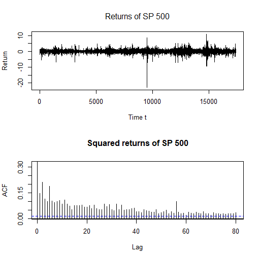
Figure 1: Returns and the sample autocorrelations of squared returns of the S&P 500.

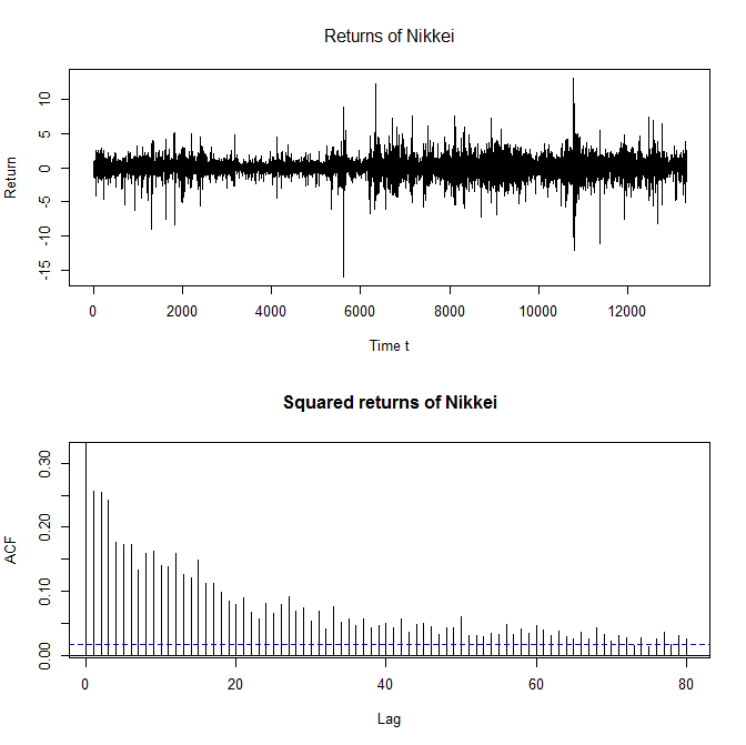
Figure 3: Returns and the sample autocorrelations of squared returns of the Nikkei.

A long-range memory property of the stock market returns series was largely investigated by Ding et al., (1993) which shown that there are more correlation beetwen power transformation of the absolute return $|r_{t}|^{v}$ ($v>0$) than returns themselves (see also Beran et al., (2013), Palma, (2007), Baillie et al., (1996) and Ling and Li, (1997)). We choose here the case where $v=2$ which corresponds to the squared returns $(r_{t}^{2})_{t\geq 1}$ process. The mean and the standard deviation of $(r_{t}^{2})_{t\geq 1}$ are $0,9347$ and $5,0036$ (resp. $1,6167$ and $5,4759$) for the S&P 500 (resp. the Nikkei) index. Following a similar way as in Ling, (2003) we denote by $(X_{t})_{t\geq 1}$ the centered series of the squared returns, that is, $X_{t}=r_{t}^{2}-0,9347$ (resp. $X_{t}=r_{t}^{2}-1,6167$) for the S&P 500 (resp. the Nikkei) index. Figure 1 (resp. Figure 3) plots the returns and the sample autocorrelations of $(X_{t})_{t\geq 1}$ of the S&P 500 (resp. of the Nikkei). The centered squared returns $(X)_{t\geq 1}$ have significant positive autocorrelations at least up to lag 80 (see Figure 1 and Figure 3) which confirm the claim that stock market returns have long-term memory (see for instance Ding et al., (1993), for more details).

We first fit a FARIMA$(1,d_{0},1)$ model defined in (21) to the process $(X)_{t\geq 1}$ of the S&P 500 and the Nikkei returns. Let $\hat{\theta}_{n}^{\mathrm{SP500}}$ and $\hat{\theta}_{n}^{\mathrm{Nikkei}}$ be respectively the least squares estimators of the parameter $\theta_{0}=(a,b,d_{0})$ for the model (21) in the case of the S&P 500 and the Nikkei. The least squares estimators were obtained as

$$\hat{\theta}_{n}^{\mathrm{SP500}}=\left(\begin{array}[]{ccc}-0.3371&[0.1105]&(0.0023)\\ -0.1795&[0.0788]&(0.0227)\\ \quad 0.2338&[0.0367]&(0.0000)\end{array}\right)\text{ and }\hat{\sigma}_{\epsilon}^{2}=22.9076\times 10^{-8}$$

and

$$\hat{\theta}_{n}^{\mathrm{Nikkei}}=\left(\begin{array}[]{ccc}-0.0217&[0.1105]&(0.9528)\\ \quad 0.1579&[0.0788]&(0.6050)\\ \quad 0.3217&[0.0367]&(0.0000)\end{array}\right)\text{ and }\hat{\sigma}_{\epsilon}^{2}=25.6844\times 10^{-8},$$ (28)

where the estimated asymptotic standard errors obtained from $\Sigma_{\hat{\theta}}:=J^{-1}IJ^{-1}$ (respectively the $p$-values), of the estimated parameters (first column), are given into brackets (respectively in parentheses). Note that for these series, the estimated coefficients $|\hat{a}_{n}|$ and $|\hat{b}_{n}|$ are smaller than one. This is in accordance with the assumptions that the power series $a_{\theta}^{-1}$ and $b_{\theta}^{-1}$ are well defined (remind that the moving average polynomial is denoted $b_{\theta}$ and the autoregressive polynomials $a_{\theta}$). We also observe that the estimated long-range dependence coefficients $\hat{d}_{n}$ is significant for any reasonable asymptotic level and is inside $]-0.5,0.5[$. So we think that the assumption (A2) is satisfied and thus our asymptotic normality theorem on the residual autocorrelations can be applied.

Concerning the S&P 500, the estimators of the parameters $a$ and $b$ are significant whereas it is not the case for the Nikkei (see (28)). In the Nikkei case, the coefficients could reasonably be set to zero. So we adjust a FARIMA$(0,d_{0},0)$ for the squares of Nikkei returns and (28) is reduced as

$$\hat{\theta}_{n}^{\mathrm{Nikkei}}=\left(\begin{array}[]{ccc}0.2132&[0.0259]&(0.0000)\end{array}\right)\text{ and }\hat{\sigma}_{\epsilon}^{2}=25.9793\times 10^{-8}.$$

We thus apply portmanteau tests to the residuals of FARIMA$(1,d_{0},1)$ (resp. FARIMA$(0,d_{0},0)$) model for the process $(X)_{t\geq 1}$ of S&P 500 (resp. of Nikkei). Table 6 (resp. Table 7) displays the statistics and the $p$-values of the standard and modified versions of BP and LB tests of model (21). From Tables 6 and 7, we draw the conclusion that the strong FARIMA$(1,0.2338,1)$ and FARIMA$(0,0.2132,0)$ models are rejected but the weak FARIMA$(1,0.2338,1)$ and FARIMA$(0,0.2132,0)$ models are not rejected.

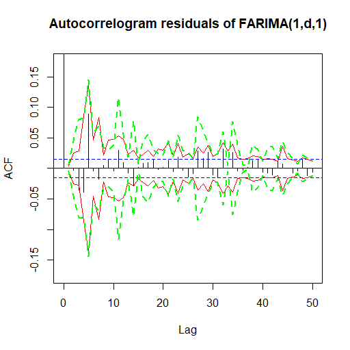
Figure 2: Autocorrelation of the FARIMA$(1,0.2338,1)$ residuals for the squares of the S&P 500 returns. The horizontal dotted lines (blue color) correspond to the 5% significant limits obtained under the strong FARIMA assumption. The solid lines (red color) and dashed lines (green color) correspond also to the 5% significant limits under the weak FARIMA assumption. The full lines correspond to the asymptotic significance limits for the residual autocorrelations obtained in Theorem 2. The dashed lines (green color) correspond to the self-normalized asymptotic significance limits for the residual autocorrelations obtained in Theorem 7.

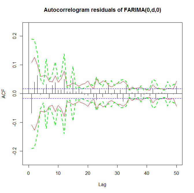
Figure 4: Autocorrelation of the FARIMA$(0,0.2132,0)$ residuals for the squares of the Nikkei returns. The horizontal dotted lines (blue color) correspond to the 5% significant limits obtained under the strong FARIMA assumption. The solid lines (red color) and dashed lines (green color) correspond also to the 5% significant limits under the weak FARIMA assumption. The full lines correspond to the asymptotic significance limits for the residual autocorrelations obtained in Theorem 2. The dashed lines (green color) correspond to the self-normalized asymptotic significance limits for the residual autocorrelations obtained in Theorem 7.

Figure 2 (resp. Figure 4) displays the residual autocorrelations and their 5% significance limits under the strong FARIMA and weak FARIMA assumptions. In view of Figures 2 and 4, the diagnostic checking of residuals does not indicate any inadequacy for the proposed tests. All of the sample autocorrelations should lie between the bands (at 95%) shown as dashed lines (green color) and solid lines (red color) for the modified tests, while the horizontal dotted (blue color) for standard test indicate that strong FARIMA is not adequate. Figure 2 (resp. Figure 4) confirms the conclusions drawn from Table 6 (resp. Table 7).

5 Figures and tables

Table 1: Empirical size (in %) of the modified and standard versions of the LB and BP tests in the case of a strong FARIMA$(0,d_{0},0)$ defined by (21) with $\theta_{0}=(0,0,d_{0})$. The nominal asymptotic level of the tests is $\alpha=5\%$. The number of replications is $N=1,000$.

$d_{0}$	Length $n$	Lag $m$	$\mathrm{{LB}}_{\textsc{sn}}$	$\mathrm{BP}_{\textsc{sn}}$	$\mathrm{{LB}}_{\textsc{w}}$	$\mathrm{BP}_{\textsc{w}}$	$\mathrm{{LB}}_{\textsc{s}}$	$\mathrm{BP}_{\textsc{s}}$
		$1$	3.3	3.3	4.6	4.5	n.a.	n.a.
		$2$	4.5	4.5	4.9	4.9	5.8	5.8
0.05	$n=1,000$	$3$	5.2	5.1	4.7	4.4	4.9	4.8
		$6$	5.8	5.8	4.6	4.5	5.1	5.0
		$12$	6.0	5.6	5.3	4.6	5.2	5.0
		$15$	5.6	5.2	4.7	4.3	5.3	4.7
		$1$	6.8	6.8	6.6	6.6	n.a.	n.a.
		$2$	6.8	6.8	6.4	6.4	7.9	7.9
0.05	$n=5,000$	$3$	6.6	6.6	5.7	5.7	5.8	5.8
		$6$	6.5	6.4	5.6	5.6	5.7	5.6
		$12$	6.4	6.4	5.3	5.3	6.0	5.9
		$15$	6.1	6.0	4.7	4.6	5.3	5.2
		$1$	4.9	4.9	5.3	5.3	n.a.	n.a.
		$2$	5.4	5.4	6.6	6.6	7.8	7.8
0.05	$n=10,000$	$3$	5.7	5.7	5.9	5.9	6.2	6.2
		$6$	5.9	5.8	4.5	4.5	4.6	4.6
		$12$	5.3	5.3	5.4	5.4	5.6	5.6
		$15$	4.4	4.3	4.8	4.8	4.9	4.9
		$1$	3.6	3.5	4.3	4.3	n.a.	n.a.
		$2$	4.7	4.7	4.7	4.7	5.8	5.7
0.20	$n=1,000$	$3$	5.2	5.0	4.3	4.3	4.9	4.7
		$6$	6.0	5.9	4.7	4.5	5.0	4.9
		$12$	5.7	5.4	5.3	4.7	5.2	4.9
		$15$	5.9	5.6	4.8	4.2	5.2	4.8
		$1$	6.6	6.6	6.5	6.5	n.a.	n.a.
		$2$	6.6	6.6	6.4	6.4	7.9	7.9
0.20	$n=5,000$	$3$	6.7	6.7	5.7	5.7	5.8	5.8
		$6$	6.3	6.3	5.6	5.6	5.7	5.5
		$12$	6.3	6.2	5.5	5.3	6.0	5.9
		$15$	6.1	5.9	4.7	4.6	5.3	5.2
		$1$	4.8	4.8	5.3	5.3	n.a.	n.a.
		$2$	5.4	5.4	6.6	6.6	7.8	7.8
0.20	$n=10,000$	$3$	5.5	5.5	5.9	5.9	6.3	6.3
		$6$	5.8	5.8	4.5	4.5	4.6	4.6
		$12$	5.4	5.3	5.5	5.5	5.6	5.6
		$15$	4.4	4.3	4.7	4.7	4.9	4.9
		$1$	3.9	3.8	4.9	4.9	n.a.	n.a.
		$2$	5.1	5.0	4.8	4.6	5.9	5.9
0.45	$n=1,000$	$3$	5.2	5.2	4.3	4.3	4.8	4.8
		$6$	6.2	6.0	4.7	4.3	4.9	4.9
		$12$	5.8	5.4	4.8	4.7	4.9	4.8
		$15$	5.6	5.5	4.5	4.2	5.0	4.8
		$1$	6.6	6.6	6.6	6.6	n.a.	n.a.
		$2$	6.7	6.7	6.5	6.5	8.0	8.0
0.45	$n=5,000$	$3$	6.6	6.6	5.7	5.7	5.8	5.8
		$6$	6.3	6.3	5.4	5.4	5.6	5.5
		$12$	6.2	6.2	5.5	5.5	6.0	5.9
		$15$	6.2	5.9	4.6	4.6	5.5	5.3
		$1$	5.0	5.0	5.3	5.3	n.a.	n.a.
		$2$	5.4	5.4	6.6	6.6	7.9	7.9
0.45	$n=10,000$	$3$	5.3	5.3	5.9	5.9	6.3	6.3
		$6$	5.8	5.8	4.7	4.6	4.7	4.7
		$12$	5.4	5.4	5.5	5.5	5.7	5.7
		$15$	4.6	4.5	4.9	4.8	4.9	4.9

Table 2: Empirical size (in %) of the modified and standard versions of the LB and BP tests in the case of a weak FARIMA$(0,d_{0},0)$ defined by (21) with $\theta_{0}=(0,0,d_{0})$ and where $\omega=0.4$, $\alpha_{1}=0.3$ and $\beta_{1}=0.3$ in (23). The nominal asymptotic level of the tests is $\alpha=5\%$. The number of replications is $N=1,000$.

$d_{0}$	Length $n$	Lag $m$	$\mathrm{{LB}}_{\textsc{sn}}$	$\mathrm{BP}_{\textsc{sn}}$	$\mathrm{{LB}}_{\textsc{w}}$	$\mathrm{BP}_{\textsc{w}}$	$\mathrm{{LB}}_{\textsc{s}}$	$\mathrm{BP}_{\textsc{s}}$
		$1$	4.4	4.4	5.4	5.4	n.a.	n.a.
		$2$	4.3	4.2	5.7	5.7	15.6	15.5
0.05	$n=1,000$	$3$	5.9	5.9	5.3	5.0	14.2	14.0
		$6$	5.2	5.1	6.0	6.0	14.6	14.4
		$12$	4.5	4.1	4.2	4.0	11.0	10.7
		$15$	4.0	3.9	4.2	3.9	11.1	10.6
		$1$	4.3	4.3	5.1	5.1	n.a.	n.a.
		$2$	4.4	4.4	5.8	5.8	16.9	16.8
0.05	$n=5,000$	$3$	5.0	5.0	5.5	5.5	16.5	16.5
		$6$	5.6	5.6	4.5	4.5	14.8	14.6
		$12$	5.1	5.1	5.0	4.9	12.6	12.5
		$15$	5.2	5.1	4.9	4.7	11.8	11.6
		$1$	5.7	5.7	5.3	5.1	n.a.	n.a.
		$2$	5.0	5.0	4.5	4.5	17.4	17.4
0.05	$n=10,000$	$3$	5.5	5.5	4.7	4.6	17.2	17.2
		$6$	5.3	5.3	5.0	5.0	14.2	14.1
		$12$	4.9	4.9	4.7	4.7	11.0	11.0
		$15$	4.9	4.8	4.7	4.6	10.2	10.2
		$1$	4.9	4.9	4.3	4.3	n.a.	n.a.
		$2$	4.0	4.0	5.7	5.6	15.5	15.4
0.20	$n=1,000$	$3$	6.0	6.0	5.0	4.8	14.0	13.8
		$6$	5.2	5.1	5.7	5.6	14.3	14.2
		$12$	4.4	4.0	4.3	4.0	10.8	10.5
		$15$	3.9	3.8	4.2	3.9	10.8	10.1
		$1$	4.3	4.3	5.0	5.0	n.a.	n.a.
		$2$	4.3	4.3	5.9	5.8	16.9	16.9
0.20	$n=5,000$	$3$	5.2	5.2	5.4	5.4	16.7	16.7
		$6$	5.6	5.5	4.6	4.5	14.8	14.7
		$12$	5.2	5.2	5.0	4.9	12.5	12.4
		$15$	5.2	5.2	4.8	4.6	11.7	11.7
		$1$	5.7	5.7	5.2	5.2	n.a.	n.a.
		$2$	5.1	5.1	4.5	4.5	17.3	17.3
0.20	$n=10,000$	$3$	5.7	5.6	4.7	4.7	17.2	17.2
		$6$	5.1	5.1	4.9	4.9	14.2	14.2
		$12$	4.8	4.8	4.7	4.7	11.0	11.0
		$15$	4.9	4.7	4.6	4.6	10.2	10.2
		$1$	4.5	4.5	5.4	5.4	n.a.	n.a.
		$2$	4.1	4.1	6.0	6.0	16.2	16.1
0.45	$n=1,000$	$3$	5.9	5.7	5.3	5.3	14.6	14.5
		$6$	5.2	4.8	5.5	5.4	14.4	14.1
		$12$	4.0	3.7	4.2	4.2	11.2	10.8
		$15$	3.8	3.7	4.3	3.9	10.6	10.4
		$1$	4.6	4.6	5.0	5.0	n.a.	n.a.
		$2$	4.3	4.3	5.9	5.9	16.7	16.7
0.45	$n=5,000$	$3$	4.9	4.9	5.4	5.4	16.8	16.7
		$6$	5.7	5.6	4.6	4.6	15.1	14.9
		$12$	5.3	5.3	5.1	5.1	12.7	12.4
		$15$	5.1	5.0	4.8	4.8	11.7	11.7
		$1$	5.7	5.7	5.2	5.2	n.a.	n.a.
		$2$	5.0	5.0	4.7	4.7	17.2	17.2
0.45	$n=10,000$	$3$	5.8	5.7	4.7	4.7	17.5	17.4
		$6$	5.1	5.1	5.0	4.9	14.3	14.3
		$12$	4.8	4.8	4.7	4.7	10.9	10.9
		$15$	4.9	4.7	4.6	4.6	10.2	10.2

Table 3: Empirical size (in %) of the modified and standard versions of the LB and BP tests in the case of weak FARIMA$(0,d_{0},0)$ defined by (21)–(23) with $\theta_{0}=(0,0,d_{0})$. The nominal asymptotic level of the tests is $\alpha=5\%$. The number of replications is $N=1,000$.

$d_{0}$	Length $n$	Lag $m$	$\mathrm{{LB}}_{\textsc{sn}}$	$\mathrm{BP}_{\textsc{sn}}$	$\mathrm{{LB}}_{\textsc{w}}$	$\mathrm{BP}_{\textsc{w}}$	$\mathrm{{LB}}_{\textsc{s}}$	$\mathrm{BP}_{\textsc{s}}$
		$1$	3.3	3.3	8.7	8.6	n.a.	n.a.
		$2$	3.8	3.7	6.1	6.1	16.9	16.9
0.05	$n=1,000$	$3$	3.5	3.5	4.8	4.7	14.8	14.8
		$6$	3.3	3.2	4.0	4.0	14.1	14.0
		$12$	1.0	0.9	2.5	2.4	13.0	12.8
		$15$	1.0	0.9	2.3	2.1	12.8	12.2
		$1$	3.9	3.9	5.3	5.3	n.a.	n.a.
		$2$	4.8	4.8	5.2	5.2	18.7	18.7
0.05	$n=5,000$	$3$	5.6	5.6	5.3	5.3	15.1	15.0
		$6$	4.8	4.8	4.3	4.3	12.4	12.4
		$12$	3.9	3.9	3.3	3.3	11.2	11.1
		$15$	3.5	3.5	2.7	2.7	10.2	10.1
		$1$	5.4	5.4	5.2	5.2	n.a.	n.a.
		$2$	5.6	5.6	5.3	5.3	18.6	18.6
0.05	$n=10,000$	$3$	4.9	4.9	5.3	5.2	16.6	16.5
		$6$	4.8	4.8	5.5	5.4	13.3	13.3
		$12$	4.1	4.0	4.0	4.0	12.2	12.2
		$15$	5.0	5.0	3.5	3.5	11.2	11.2
		$1$	3.3	3.3	4.9	4.9	n.a.	n.a.
		$2$	4.2	4.1	4.4	4.3	14.7	14.7
0.20	$n=1,000$	$3$	3.7	3.7	3.4	3.2	12.8	12.8
		$6$	3.6	3.4	2.7	2.7	12.9	12.8
		$12$	1.1	1.0	1.9	1.7	11.8	11.3
		$15$	0.9	0.6	1.8	1.7	12.0	11.5
		$1$	3.8	3.8	5.5	5.5	n.a.	n.a.
		$2$	4.7	4.7	5.1	5.1	18.8	18.8
0.20	$n=5,000$	$3$	5.8	5.8	5.2	5.2	15.0	15.0
		$6$	4.9	4.9	4.3	4.3	12.5	12.4
		$12$	3.9	3.9	3.4	3.4	11.1	11.1
		$15$	3.5	3.3	2.7	2.7	10.2	10.1
		$1$	5.4	5.4	5.1	5.1	n.a.	n.a.
		$2$	5.6	5.6	5.3	5.3	18.8	18.8
0.20	$n=10,000$	$3$	5.0	5.0	5.2	5.2	16.6	16.6
		$6$	4.8	4.8	5.4	5.4	13.3	13.3
		$12$	4.0	4.0	4.0	4.0	12.1	12.1
		$15$	5.3	5.3	3.4	3.4	11.2	11.2
		$1$	3.5	3.5	9.0	9.0	n.a.	n.a.
		$2$	4.1	4.1	5.9	5.9	17.5	17.5
0.45	$n=1,000$	$3$	3.9	3.7	5.0	4.8	15.0	14.6
		$6$	3.4	3.4	3.7	3.7	14.1	13.9
		$12$	0.9	0.9	2.0	2.0	12.9	12.2
		$15$	1.0	0.5	1.9	1.7	13.1	12.8
		$1$	4.1	4.1	5.4	5.4	n.a.	n.a.
		$2$	4.6	4.6	5.2	5.2	18.8	18.7
0.45	$n=5,000$	$3$	5.6	5.6	5.2	5.2	15.2	15.2
		$6$	5.1	5.0	4.4	4.4	12.5	12.4
		$12$	4.0	3.8	3.5	3.5	11.1	11.1
		$15$	3.5	3.5	2.6	2.6	10.0	9.9
		$1$	5.5	5.5	5.1	5.1	n.a.	n.a.
		$2$	5.6	5.6	5.3	5.3	18.7	18.6
0.45	$n=10,000$	$3$	4.7	4.7	5.2	5.2	16.6	16.6
		$6$	4.8	4.8	5.3	5.3	13.3	13.3
		$12$	4.0	4.0	4.0	4.0	12.1	12.1
		$15$	5.2	5.2	3.5	3.5	11.1	11.1

Table 4: Empirical power (in %) of the modified and standard versions of the LB and BP tests in the case of a weak FARIMA$(0,d_{0},1)$ defined by (21) with $\theta_{0}=(0.,0.2,d_{0})$ and where $\omega=0.4$, $\alpha_{1}=0.3$ and $\beta_{1}=0.3$ in (22). The nominal asymptotic level of the tests is $\alpha=5\%$. The number of replications is $N=1,000$.

$d_{0}$	Length $n$	Lag $m$	$\mathrm{{LB}}_{\textsc{sn}}$	$\mathrm{BP}_{\textsc{sn}}$	$\mathrm{{LB}}_{\textsc{w}}$	$\mathrm{BP}_{\textsc{w}}$	$\mathrm{{LB}}_{\textsc{s}}$	$\mathrm{BP}_{\textsc{s}}$
		$1$	30.1	30.1	100.0	100.0	n.a.	n.a.
		$2$	55.7	55.7	100.0	100.0	100.0	100.0
0.05	$n=5,000$	$3$	75.7	75.7	100.0	100.0	100.0	100.0
		$6$	87.1	87.1	100.0	100.0	100.0	100.0
		$12$	87.0	86.8	100.0	100.0	100.0	100.0
		$15$	87.3	87.2	100.0	100.0	100.0	100.0
		$1$	50.0	50.0	100.0	100.0	n.a.	n.a.
		$2$	79.5	79.4	100.0	100.0	100.0	100.0
0.05	$n=10,000$	$3$	95.2	95.2	100.0	100.0	100.0	100.0
		$6$	98.0	98.0	100.0	100.0	100.0	100.0
		$12$	98.6	98.6	100.0	100.0	100.0	100.0
		$15$	99.0	99.0	100.0	100.0	100.0	100.0
		$1$	98.2	98.2	99.9	99.9	n.a.	n.a.
		$2$	94.6	94.6	99.5	99.5	100.0	100.0
0.20	$n=5,000$	$3$	92.3	92.3	99.6	99.6	100.0	100.0
		$6$	91.0	91.0	99.6	99.6	100.0	100.0
		$12$	88.8	88.7	99.8	99.8	100.0	100.0
		$15$	88.6	88.6	99.8	99.8	100.0	100.0
		$1$	99.7	99.7	100.0	100.0	n.a.	n.a.
		$2$	99.2	99.2	100.0	100.0	100.0	100.0
0.20	$n=10,000$	$3$	99.3	99.2	100.0	100.0	100.0	100.0
		$6$	98.8	98.8	100.0	100.0	100.0	100.0
		$12$	99.3	99.3	100.0	100.0	100.0	100.0
		$15$	99.3	99.3	100.0	100.0	100.0	100.0
		$1$	98.2	98.2	99.8	99.8	n.a.	n.a.
		$2$	94.4	94.3	99.5	99.5	100.0	100.0
0.45	$n=5,000$	$3$	92.4	92.4	99.6	99.6	100.0	100.0
		$6$	90.9	90.8	99.6	99.6	100.0	100.0
		$12$	88.9	88.9	99.8	99.8	100.0	100.0
		$15$	88.8	88.5	99.8	99.8	100.0	100.0
		$1$	99.7	99.7	100.0	100.0	n.a.	n.a.
		$2$	99.0	99.0	100.0	100.0	100.0	100.0
0.45	$n=10,000$	$3$	99.2	99.2	100.0	100.0	100.0	100.0
		$6$	98.9	98.9	100.0	100.0	100.0	100.0
		$12$	99.3	99.3	100.0	100.0	100.0	100.0
		$15$	99.3	99.3	100.0	100.0	100.0	100.0

Table 5: Empirical power (in %) of the modified and standard versions of the LB and BP tests in the case of a weak FARIMA$(0,d_{0},1)$ defined by (21)–(23) with $\theta_{0}=(0.,0.2,d_{0})$. The nominal asymptotic level of the tests is $\alpha=5\%$. The number of replications is $N=1,000$.

$d_{0}$	Length $n$	Lag $m$	$\mathrm{{LB}}_{\textsc{sn}}$	$\mathrm{BP}_{\textsc{sn}}$	$\mathrm{{LB}}_{\textsc{w}}$	$\mathrm{BP}_{\textsc{w}}$	$\mathrm{{LB}}_{\textsc{s}}$	$\mathrm{BP}_{\textsc{s}}$
		$1$	20.3	20.3	99.9	99.9	n.a.	n.a.
		$2$	56.7	56.6	99.9	99.9	99.9	99.9
0.05	$n=5,000$	$3$	69.1	69.1	99.9	99.9	99.9	99.9
		$6$	75.9	75.9	99.9	99.9	99.9	99.9
		$12$	71.9	71.4	99.9	99.9	99.9	99.9
		$15$	68.5	68.0	99.9	99.9	99.9	99.9
		$1$	60.0	60.0	100.0	100.0	n.a.	n.a.
		$2$	81.8	81.8	100.0	100.0	100.0	100.0
0.05	$n=10,000$	$3$	90.3	90.3	100.0	100.0	100.0	100.0
		$6$	93.9	93.9	100.0	100.0	100.0	100.0
		$12$	93.8	93.8	100.0	100.0	100.0	100.0
		$15$	93.7	93.7	100.0	100.0	100.0	100.0
		$1$	92.3	92.3	99.9	99.9	n.a.	n.a.
		$2$	86.1	86.0	98.6	98.6	99.8	99.8
0.20	$n=5,000$	$3$	82.3	82.3	99.2	99.1	99.8	99.8
		$6$	80.0	80.0	98.9	98.9	99.9	99.9
		$12$	73.1	72.8	98.7	98.7	99.6	99.6
		$15$	68.3	68.0	98.4	98.4	99.5	99.5
		$1$	99.2	99.2	100.0	100.0	n.a.	n.a.
		$2$	96.4	96.4	100.0	100.0	100.0	100.0
0.20	$n=10,000$	$3$	94.6	94.6	100.0	100.0	100.0	100.0
		$6$	95.1	95.1	100.0	100.0	100.0	100.0
		$12$	95.2	95.2	100.0	100.0	100.0	100.0
		$15$	94.0	94.0	100.0	100.0	100.0	100.0
		$1$	92.4	92.4	99.9	99.9	n.a.	n.a.
		$2$	85.6	85.6	98.6	98.6	99.8	99.8
0.45	$n=5,000$	$3$	82.1	82.0	99.3	99.3	99.8	99.8
		$6$	80.3	80.3	98.9	98.9	99.9	99.9
		$12$	73.0	72.7	98.7	98.7	99.6	99.6
		$15$	68.2	68.1	98.4	98.4	99.5	99.5
		$1$	99.2	99.2	100.0	100.0	n.a.	n.a.
		$2$	96.4	96.4	100.0	100.0	100.0	100.0
0.45	$n=10,000$	$3$	94.8	94.8	100.0	100.0	100.0	100.0
		$6$	95.2	95.2	100.0	100.0	100.0	100.0
		$12$	95.0	95.0	100.0	100.0	100.0	100.0
		$15$	94.0	94.0	100.0	100.0	100.0	100.0

Table 6: Modified and standard versions of portmanteau tests to check the null hypothesis that the S&P 500 squared returns follow a FARIMA$(1,0.2338,1)$ model (21).

Lag $m$		1	2	3	4	5	6	7
$\hat{\rho}(m)$		0.0002	-0.0033	-0.0350	-0.0393	0.0893	-0.0040	-0.0179
$\mathrm{LB}_{\textsc{sn}}$		0.0653	18.150	41.924	58.057	186.72	313.78	341.38
$\mathrm{BP}_{\textsc{sn}}$		0.0653	18.146	41.912	58.037	186.64	313.64	341.20
$\mathrm{LB}_{\textsc{w}}$		0.0008	0.1885	21.445	48.248	186.95	187.23	192.77
$\mathrm{BP}_{\textsc{w}}$		0.0008	0.1884	21.439	48.232	186.88	187.15	192.67
$\mbox{p}_{\textsc{w}}^{\textsc{lb}}$		0.8525	0.6985	0.0916	0.3137	0.0678	0.0717	0.0752
$\mbox{p}_{\textsc{w}}^{\textsc{bp}}$		0.8525	0.6986	0.0917	0.3138	0.0679	0.0718	0.0753
$\mbox{p}_{\textsc{s}}^{\textsc{lb}}$		n.a.	n.a.	n.a.	0.0000	0.0000	0.0000	0.0000
$\mbox{p}_{\textsc{s}}^{\textsc{bp}}$		n.a.	n.a.	n.a.	0.0000	0.0000	0.0000	0.0000
Lag $m$		8	9	10	11	12	13	14
$\hat{\rho}(m)$		0.0047	0.0137	-0.0040	0.0295	0.0093	-0.0077	-0.0286
$\mathrm{LB}_{\textsc{sn}}$		397.27	397.38	415.22	465.52	468.76	567.87	573.02
$\mathrm{BP}_{\textsc{sn}}$		397.04	397.13	414.93	465.17	468.33	567.38	572.49
$\mathrm{LB}_{\textsc{w}}$		193.16	196.42	196.69	211.82	213.31	214.34	228.55
$\mathrm{BP}_{\textsc{w}}$		193.09	196.34	196.61	211.74	213.22	214.25	228.45
$\mbox{p}_{\textsc{w}}^{\textsc{lb}}$		0.0758	0.0786	0.0986	0.1053	0.1148	0.1226	0.1047
$\mbox{p}_{\textsc{w}}^{\textsc{bp}}$		0.0758	0.0787	0.0987	0.1054	0.1150	0.1228	0.1048
$\mbox{p}_{\textsc{s}}^{\textsc{lb}}$		0.0000	0.0000	0.0000	0.0000	0.0000	0.0000	0.0000
$\mbox{p}_{\textsc{s}}^{\textsc{bp}}$		0.0000	0.0000	0.0000	0.0000	0.0000	0.0000	0.0000
Lag $m$		15	16	17	18	19	20	21
$\hat{\rho}(m)$		0.0021	0.0086	0.0097	0.0137	-0.0023	0.0016	0.0132
$\mathrm{LB}_{\textsc{sn}}$		588.61	701.16	738.23	738.58	749.24	778.88	788.01
$\mathrm{BP}_{\textsc{sn}}$		588.04	700.44	737.42	737.73	748.33	777.90	786.97
$\mathrm{LB}_{\textsc{w}}$		228.63	229.91	231.54	234.83	234.92	234.97	238.00
$\mathrm{BP}_{\textsc{w}}$		228.52	229.80	231.44	234.72	234.81	234.86	237.89
$\mbox{p}_{\textsc{w}}^{\textsc{lb}}$		0.1079	0.1113	0.2212	0.2138	0.2127	0.2169	0.2324
$\mbox{p}_{\textsc{w}}^{\textsc{bp}}$		0.1080	0.1114	0.2214	0.2140	0.2130	0.2171	0.2327
$\mbox{p}_{\textsc{s}}^{\textsc{lb}}$		0.0000	0.0000	0.0000	0.0000	0.0000	0.0000	0.0000
$\mbox{p}_{\textsc{s}}^{\textsc{bp}}$		0.0000	0.0000	0.0000	0.0000	0.0000	0.0000	0.0000

Table 7: Modified and standard versions of portmanteau tests to check the null hypothesis that the Nikkei squared returns follow a FARIMA$(0,0.2132,0)$ model as in (21) with $a=b=0$.

Lag $m$		1	2	3	4	5	6	7
$\hat{\rho}(m)$		-0.0678	0.0400	0.0634	-0.0022	0.0165	0.0320	-0.0158
$\mathrm{LB}_{\textsc{sn}}$		5.7332	29.005	34.758	34.779	66.692	288.57	324.46
$\mathrm{BP}_{\textsc{sn}}$		5.7319	28.997	34.745	34.764	66.657	288.40	324.24
$\mathrm{LB}_{\textsc{w}}$		61.211	82.507	136.13	136.20	139.84	153.46	156.78
$\mathrm{BP}_{\textsc{w}}$		61.198	82.487	136.09	136.16	139.76	153.41	156.73
$\mbox{p}_{\textsc{w}}^{\textsc{lb}}$		0.1086	0.2186	0.1830	0.2551	0.3002	0.3519	0.3609
$\mbox{p}_{\textsc{w}}^{\textsc{bp}}$		0.1086	0.2187	0.1831	0.2552	0.3003	0.3521	0.3611
$\mbox{p}_{\textsc{s}}^{\textsc{lb}}$		n.a.	0.0000	0.0000	0.0000	0.0000	0.0000	0.0000
$\mbox{p}_{\textsc{s}}^{\textsc{bp}}$		n.a.	0.0000	0.0000	0.0000	0.0000	0.0000	0.0000
Lag $m$		8	9	10	11	12	13	14
$\hat{\rho}(m)$		0.0295	0.0384	0.0121	0.0133	0.0503	0.0076	0.0068
$\mathrm{LB}_{\textsc{sn}}$		387.88	512.70	575.09	600.81	791.67	808.20	808.27
$\mathrm{BP}_{\textsc{sn}}$		387.59	512.28	574.57	600.22	790.83	807.29	807.30
$\mathrm{LB}_{\textsc{w}}$		168.41	188.08	190.01	192.36	226.12	226.89	227.50
$\mathrm{BP}_{\textsc{w}}$		168.35	187.10	189.93	192.29	225.10	226.76	227.39
$\mbox{p}_{\textsc{w}}^{\textsc{lb}}$		0.3627	0.3757	0.3802	0.3825	0.3320	0.3447	0.3526
$\mbox{p}_{\textsc{w}}^{\textsc{bp}}$		0.3629	0.3759	0.3804	0.3827	0.3323	0.3450	0.3529
$\mbox{p}_{\textsc{s}}^{\textsc{lb}}$		0.0000	0.0000	0.0000	0.0000	0.0000	0.0000	0.0000
$\mbox{p}_{\textsc{s}}^{\textsc{bp}}$		0.0000	0.0000	0.0000	0.0000	0.0000	0.0000	0.0000
Lag $m$		15	16	17	18	19	20	21
$\hat{\rho}(m)$		0.0538	0.0073	0.0173	0.0067	-0.0027	-0.0057	0.0153
$\mathrm{LB}_{\textsc{sn}}$		839.87	842.24	842.31	845.36	885.74	935.70	946.03
$\mathrm{BP}_{\textsc{sn}}$		838.80	841.10	841.11	844.10	884.35	934.15	944.40
$\mathrm{LB}_{\textsc{w}}$		266.16	266.88	270.85	271.45	271.56	271.99	275.13
$\mathrm{BP}_{\textsc{w}}$		265.99	266.71	270.68	271.28	271.38	271.82	274.94
$\mbox{p}_{\textsc{w}}^{\textsc{lb}}$		0.3105	0.3163	0.3161	0.3264	0.3289	0.3329	0.3366
$\mbox{p}_{\textsc{w}}^{\textsc{bp}}$		0.3108	0.3166	0.3165	0.3268	0.3293	0.3333	0.3369
$\mbox{p}_{\textsc{s}}^{\textsc{lb}}$		0.0000	0.0000	0.0000	0.0000	0.0000	0.0000	0.0000
$\mbox{p}_{\textsc{s}}^{\textsc{bp}}$		0.0000	0.0000	0.0000	0.0000	0.0000	0.0000	0.0000

Appendix A Supplemental material: Proofs

The following proofs are quite technical and are adaptations of the arguments used in Francq and Zakoïan, (1998), Francq et al., (2005) and Boubacar Maïnassara and Saussereau, (2018).

The results of Boubacar Maïnassara et al., (2019) which will be needed for all the proofs are collected in the following Subsection A.1 in order to have a self-containing paper.

In all our proofs, $K$ is a positive constant that may vary from line to line.

A.1 Preliminary results

In this subsection, we shall give some results on estimations of the coefficients of formal power series that will arise in our study.

We begin by recalling the following properties on power series. If for $|z|\leq R$, the power series $f(z)=\sum_{i\geq 0}a_{i}z^{i}$ and $g(z)=\sum_{i\geq 0}b_{i}z^{i}$ are well defined, then one has $(fg)(z)=\sum_{i\geq 0}c_{i}z^{i}$ is also well defined for $|z|\leq R$ with the sequence $(c_{i})_{i\geq 0}$ which is given by $c=a\ast b$ where $\ast$ denotes the convolution product between $a$ and $b$ defined by $c_{i}=\sum_{k=0}^{i}a_{k}b_{i-k}=\sum_{k=0}^{i}a_{i-k}b_{k}$. We will make use of the Young inequality that states that if the sequence $a\in\ell^{r_{1}}$ and $b\in\ell^{r_{2}}$ and such that $\frac{1}{r_{1}}+\frac{1}{r_{2}}=1+\frac{1}{r}$ with $1\leq r_{1},r_{2},r\leq\infty$, then

$$\left\|a\ast b\right\|_{\ell^{r}}\leq\left\|a\right\|_{\ell^{r_{1}}}\times\left\|b\right\|_{\ell^{r_{2}}}.$$

Now we come back to the power series that arise in our context. Remind that for the true value of the parameter,

$$a_{\theta_{0}}(L)(1-L)^{d_{0}}X_{t}=b_{\theta_{0}}(L)\epsilon_{t}.$$ (30)

Thanks to the assumptions on the moving average polynomials $b_{\theta}$ and the autoregressive polynomials $a_{\theta}$, the power series $a_{\theta}^{-1}$ and $b_{\theta}^{-1}$ are well defined.

Thus the functions $\epsilon_{t}(\theta)$ defined in (2) can be written as

$$\epsilon_{t}(\theta) =b^{-1}_{\theta}(L)a_{\theta}(L)(1-L)^{d}X_{t}$$ (31)

$$=b^{-1}_{\theta}(L)a_{\theta}(L)(1-L)^{d-d_{0}}a^{-1}_{\theta_{0}}(L)b_{\theta_{0}}(L)\epsilon_{t}$$ (32)

and if we denote $\gamma(\theta)=(\gamma_{i}(\theta))_{i\geq 0}$ the sequence of coefficients of the power series $b^{-1}_{\theta}(z)a_{\theta}(z)(1-z)^{d}$, we may write for all $t\in\mathbb{Z}$:

$$\epsilon_{t}(\theta) =\sum_{i\geq 0}\gamma_{i}(\theta)X_{t-i}.$$ (33)

In the same way, by (31) one has

$$X_{t} =(1-L)^{-d}a^{-1}_{\theta}(L)b_{\theta}(L)\epsilon_{t}(\theta)$$

and if we denote $\eta(\theta)=(\eta_{i}(\theta))_{i\geq 0}$ the coefficients of the power series $(1-z)^{-d}a^{-1}_{\theta}(z)b_{\theta}(z)$ one has

$$X_{t} =\sum_{i\geq 0}\eta_{i}(\theta)\epsilon_{t-i}(\theta)\ .$$ (34)

We strength the fact that $\gamma_{0}(\theta)=\eta_{0}(\theta)=1$ for all $\theta$.

For large $j$, Hallin et al., (1999) have shown that uniformly in $\theta$ the sequences $\gamma(\theta)$ and $\eta(\theta)$ satisfy

$$\frac{\partial^{k}\gamma_{j}(\theta)}{\partial\theta_{i_{1}}\cdots\partial\theta_{i_{k}}}=\mathrm{O}\left(j^{-1-d}\left\{\log(j)\right\}^{k}\right),\text{ for }k=0,1,2,3,$$ (35)

and

$$\frac{\partial^{k}\eta_{j}(\theta)}{\partial\theta_{i_{1}}\cdots\partial\theta_{i_{k}}}=\mathrm{O}\left(j^{-1+d}\left\{\log(j)\right\}^{k}\right),\text{ for }k=0,1,2,3.$$ (36)

One difficulty that has to be addressed is that (33) includes the infinite past $(X_{t-i})_{i\geq 0}$ whereas only a finite number of observations $(X_{t})_{1\leq t\leq n}$ are available to compute the estimators defined in (4). The simplest solution is truncation which amounts to setting all unobserved values equal to zero. Thus, for all $\theta\in\Theta$ and $1\leq t\leq n$ one defines

$$\tilde{\epsilon}_{t}(\theta)=\sum_{i=0}^{t-1}\gamma_{i}(\theta)X_{t-i}=\sum_{i\geq 0}\gamma_{i}^{t}(\theta)X_{t-i}$$ (37)

where the truncated sequence $\gamma^{t}(\theta)=(\gamma_{i}^{t}(\theta))_{i\geq 0}$ is defined by

$$\gamma_{i}^{t}(\theta)=\left\{\begin{array}[]{rl}\gamma_{i}(\theta)&\text{ if }\ 0\leq i\leq t-1\ ,\\ 0&\text{ otherwise.}\end{array}\right.$$

Since our assumptions are made on the noise in $(\ref{FARIMA})$, it will be useful to express the random variables $\epsilon_{t}(\theta)$ and its partial derivatives with respect to $\theta$, as a function of $(\epsilon_{t-i})_{i\geq 0}$.

From (32), there exists a sequence $\lambda(\theta)=(\lambda_{i}(\theta))_{i\geq 0}$ such that

$$\epsilon_{t}(\theta)=\sum_{i=0}^{\infty}\lambda_{i}\left(\theta\right)\epsilon_{t-i}$$ (38)

where the sequence $\lambda(\theta)$ is given by the sequence of the coefficients of the power series $b^{-1}_{\theta}(z)a_{\theta}(z)(1-z)^{d-d_{0}}a^{-1}_{\theta_{0}}(z)b_{\theta_{0}}(z)$. Consequently $\lambda(\theta)=\gamma(\theta)\ast\eta(\theta_{0})$ or, equivalently,

$$\lambda_{i}(\theta) =\sum_{j=0}^{i}\gamma_{j}(\theta)\eta_{i-j}(\theta_{0}).$$ (39)

As in Hualde and Robinson, (2011), it can be shown using Stirling’s approximation that there exists a positive constant $K$ such that

$$\sup_{\theta\in\Theta_{\delta}}\left|\lambda_{i}(\theta)\right|\leq K\sup_{d\in[d_{1},d_{2}]}i^{-1-(d-d_{0})}\leq Ki^{-1-(d_{1}-d_{0})}\ .$$ (40)

Equation (38) and Inequality (40) imply that for all $\theta\in\Theta$ the random variable $\epsilon_{t}(\theta)$ belongs to $\mathbb{L}^{2}$, that the sequence $(\epsilon_{t}(\theta))_{t}$ is an ergodic sequence and that for all $t\in\mathbb{Z}$ the function $\epsilon_{t}(\cdot)$ is a continuous function. We proceed in the same way as regard to the derivatives of $\epsilon_{t}(\theta)$. More precisely, for any $\theta\in\Theta$, $t\in\mathbb{Z}$ and $1\leq k,l\leq p+q+1$ there exists sequences $\overset{\textbf{.}}{\lambda}_{k}(\theta)=(\overset{\textbf{.}}{\lambda}_{i,k}(\theta))_{i\geq 1}$ and $\overset{\textbf{..}}{\lambda}_{k,l}(\theta)=(\overset{\textbf{..}}{\lambda}_{i,k,l}(\theta))_{i\geq 1}$ such that

$$\frac{\partial\epsilon_{t}(\theta)}{\partial\theta_{k}} =\sum_{i=1}^{\infty}\overset{\textbf{.}}{\lambda}_{i,k}\left(\theta\right)\epsilon_{t-i}$$ (41)

$$\frac{\partial^{2}\epsilon_{t}(\theta)}{\partial\theta_{k}\partial\theta_{l}} =\sum_{i=1}^{\infty}\overset{\textbf{..}}{\lambda}_{i,k,l}\left(\theta\right)\epsilon_{t-i}.$$ (42)

Of course it holds that $\overset{\textbf{.}}{\lambda}_{k}(\theta)=\frac{\partial\gamma(\theta)}{\partial\theta_{k}}\ast\eta(\theta_{0})$ and $\overset{\textbf{..}}{\lambda}_{k,l}(\theta)=\frac{\partial^{2}\gamma(\theta)}{\partial\theta_{k}\partial\theta_{l}}\ast\eta(\theta_{0})$.

Similarly we have

$$\tilde{\epsilon}_{t}(\theta) =\sum_{i=0}^{\infty}\lambda_{i}^{t}\left(\theta\right)\epsilon_{t-i},$$ (43)

$$\frac{\partial\tilde{\epsilon}_{t}(\theta)}{\partial\theta_{k}} =\sum_{i=1}^{\infty}\overset{\textbf{.}}{\lambda}_{i,k}^{t}\left(\theta\right)\epsilon_{t-i},$$ (44)

$$\frac{\partial^{2}\tilde{\epsilon}_{t}(\theta)}{\partial\theta_{k}\partial\theta_{l}} =\sum_{i=1}^{\infty}\overset{\textbf{..}}{\lambda}_{i,k,l}^{t}\left(\theta\right)\epsilon_{t-i},$$ (45)

where $\lambda^{t}(\theta)=\gamma^{t}(\theta)\ast\eta(\theta_{0})$, $\overset{\textbf{.}}{\lambda}^{t}_{k}(\theta)=\frac{\partial\gamma^{t}(\theta)}{\partial\theta_{k}}\ast\eta(\theta_{0})$ and $\overset{\textbf{..}}{\lambda}^{t}_{k,l}(\theta)=\frac{\partial^{2}\gamma^{t}(\theta)}{\partial\theta_{k}\partial\theta_{l}}\ast\eta(\theta_{0})$.

In order to handle the truncation error $\epsilon_{t}(\theta)-\tilde{\epsilon}_{t}(\theta)$, one needs some information on the sequence $\lambda(\theta)-\lambda^{t}(\theta)$. In Boubacar Maïnassara et al., (2019) the following two lemmas are proved.

Lemma 1.

For $2\leq r\leq\infty$ and $1\leq k,l\leq p+q+1$, we have

$$\parallel\lambda\left(\theta\right)-\lambda^{t}\left(\theta\right)\parallel_{\ell^{r}}\ =\mathrm{O}\left(t^{-1+\frac{1}{r}-(d-max(d_{0},0))}\right),$$

$$\parallel\overset{\textbf{.}}{\lambda}_{k}\left(\theta\right)-\overset{\textbf{.}}{\lambda}_{k}^{t}\left(\theta\right)\parallel_{\ell^{r}}\ =\mathrm{O}\left(t^{-1+\frac{1}{r}-(d-max(d_{0},0))}\right)$$

and

$$\parallel\overset{\textbf{..}}{\lambda}_{k,l}\left(\theta\right)-\overset{\textbf{..}}{\lambda}_{k,l}^{t}\left(\theta\right)\parallel_{\ell^{r}}\ =\mathrm{O}\left(t^{-1+\frac{1}{r}-(d-max(d_{0},0))}\right)$$

for any $\theta\in\Theta_{\delta}$ if $d_{0}\leq 0$ and for $\theta$ with non-negative memory parameter $d$ if $d_{0}>0$.

Remark 4.

The above lemma implies that the sequence $\overset{\textbf{.}}{\lambda}_{k}\left(\theta_{0}\right)-\overset{\textbf{.}}{\lambda^{t}}_{k}\left(\theta_{0}\right)$ is bounded and more precisely there exists $K$ such that

$$\sup_{j\geq 1}\left|\overset{\textbf{.}}{\lambda}_{j,k}\left(\theta_{0}\right)-\overset{\textbf{.}}{\lambda^{t}}_{j,k}\left(\theta_{0}\right)\right| \leq\frac{K}{t^{1+\min(d_{0},0)}}$$ (46)

for any $t\geq 1$ and any $1\leq k\leq p+q+1$.

Remark 5.

In order to prove our asymptotic results, it will be convenient to give an upper bound for the norms of the sequences introduced in Lemma 1 valid for any $\theta\in\Theta_{\delta}$. Since $d_{1}-d_{0}>-1/2$, Estimation (40) entails that for any $r\geq 2$,

$$\parallel\lambda\left(\theta\right)-\lambda^{t}\left(\theta\right)\parallel_{\ell^{r}}\ =\mathrm{O}\left(t^{-1+\frac{1}{r}-(d_{1}-d_{0})}\right),\ \ \ \forall\theta\in\Theta_{\delta}.$$

This can easily be seen since $\parallel\lambda(\theta)-\lambda^{t}(\theta)\parallel_{\ell^{r}}\leq K(\sum_{i\geq t}i^{-r-r(d_{1}-d_{0})})^{1/r}\leq Kt^{-1+1/r-(d_{1}-d_{0})}$. As in Hallin et al., (1999), the coefficients $\overset{\textbf{.}}{\lambda}_{j,k}(\theta)$ and $\overset{\textbf{..}}{\lambda}_{j,k,l}(\theta)$ are $\mathrm{O}(j^{-1-(d-d_{0})+\zeta})$ for any small enough $\zeta>0$, so we have

$$\parallel\overset{\textbf{.}}{\lambda}_{k}\left(\theta\right)-\overset{\textbf{.}}{\lambda}_{k}^{t}\left(\theta\right)\parallel_{\ell^{r}}\ =\mathrm{O}\left(t^{-1+\frac{1}{r}-(d_{1}-d_{0})+\zeta}\right)$$

and

$$\parallel\overset{\textbf{..}}{\lambda}_{k,l}\left(\theta\right)-\overset{\textbf{..}}{\lambda}_{k,l}^{t}\left(\theta\right)\parallel_{\ell^{r}}\ =\mathrm{O}\left(t^{-1+\frac{1}{r}-(d_{1}-d_{0})+\zeta}\right)$$

for any $r\geq 2$, any $1\leq k,l\leq p+q+1$ and all $\theta\in\Theta_{\delta}$.

Lemma 2.

For any $2\leq r\leq\infty$, $1\leq k\leq p+q+1$ and $\theta\in\Theta$, there exists a constant $K$ such that we have

$$\parallel\lambda_{k}^{t}\left(\theta\right)\parallel_{\ell^{r}} \leq K$$

$$\text{and}\quad\parallel\overset{\textbf{.}}{\lambda}_{k}^{t}\left(\theta\right)\parallel_{\ell^{r}} \leq K.$$

A.2 Proof of Proposition 1

First we remark that the asymptotic normality of the joint distribution of $\sqrt{n}(\hat{\theta}_{n}^{\prime}-\theta_{0}^{{}^{\prime}},\gamma_{m}^{{}^{\prime}})^{{}^{\prime}}$ can be established along the same lines as the proof of Theorem 2 in Boubacar Maïnassara et al., (2019). The detailed proof is omitted. From (6) and (11) we have

$$\sqrt{n}\begin{pmatrix}\hat{\theta}_{n}-\theta_{0}\vspace{0.2cm}\\ \gamma_{m}\end{pmatrix} =\frac{1}{\sqrt{n}}\sum_{t=1}^{n}\begin{pmatrix}-2J^{-1}(\theta_{0})\epsilon_{t}\frac{\partial}{\partial\theta}\epsilon_{t}(\theta_{0})\vspace{0.2cm}\\ (\epsilon_{t-1},\dots,\epsilon_{t-m})^{{}^{\prime}}\epsilon_{t}\end{pmatrix}+\begin{pmatrix}\mathrm{o}_{\mathbb{P}}(1)\\ \mathbf{0}_{m}\end{pmatrix}$$

$$=\frac{1}{\sqrt{n}}\sum_{t=1}^{n}U_{t}+\mathrm{o}_{\mathbb{P}}(1),$$

where $\mathbf{0}_{m}$ is the vector of $\mathbb{R}^{m\times 1}$ with zero components. It is clear that $U_{t}$ is a measurable function of $\epsilon_{t},\epsilon_{t-1},\dots$ Thus by using the same arguments as in Boubacar Maïnassara et al., (2019) (see proof of Theorem 2), the central limit theorem (CLT) for strongly mixing processes $(U_{t})_{t\in\mathbb{Z}}$ of Herrndorf, (1984) implies that $({1}/{\sqrt{n}})\sum_{t=1}^{n}U_{t}$ has a limiting normal distribution with mean 0 and covariance matrix $\Xi$.

For $i\geq 1$, we denote ${\Lambda}_{i}(\theta_{0})=(\overset{\textbf{.}}{\lambda}_{i,1}(\theta_{0}),\dots,\overset{\textbf{.}}{\lambda}_{i,p+q+1}(\theta_{0}))^{\prime}$. From (41) we deduce that

$$\frac{\partial\epsilon_{t}(\theta_{0})}{\partial\theta} =\sum_{i=1}^{\infty}{\Lambda}_{i}(\theta_{0})\epsilon_{t-i}.$$ (47)

In view of (11) and (47), by applying the CLT for mixing processes we directly obtain

$$\Sigma_{\hat{\theta}} =\lim_{n\rightarrow\infty}\mathrm{Var}\left(2J^{-1}\frac{1}{\sqrt{n}}\sum_{t=1}^{n}\epsilon_{t}\frac{\partial}{\partial\theta}\epsilon_{t}(\theta_{0})\right):=J^{-1}IJ^{-1}$$

$$=4J^{-1}\sum_{\ell,\ell^{\prime}=1}^{\infty}{\Lambda}_{\ell}\left(\theta_{0}\right){\Lambda^{\prime}}_{\ell^{\prime}}\left(\theta_{0}\right)\sum_{h=-\infty}^{\infty}\mathbb{E}\left(\epsilon_{t}\epsilon_{t-\ell}\epsilon_{t-h}\epsilon_{t-\ell^{\prime}-h}\right)J^{-1}$$

$$=4J^{-1}\sum_{\ell,\ell^{\prime}=1}^{\infty}{\Lambda}_{\ell}\left(\theta_{0}\right){\Lambda^{\prime}}_{\ell^{\prime}}\left(\theta_{0}\right)\Gamma(\ell,\ell^{\prime})J^{-1},$$

which gives the first block of the asymptotic covariance matrix of Proposition 1.

By the stationarity of $(\epsilon_{t})_{t\in\mathbb{Z}}$ and Lebesgue’s dominated convergence theorem, we obtain the $(\ell,\ell^{{}^{\prime}})$-th entry of the matrix $\Gamma_{m,m}$:

$$\lim_{n\rightarrow\infty}\mathrm{Cov}(\sqrt{n}\gamma(\ell),\sqrt{n}\gamma(\ell^{{}^{\prime}})) =\lim_{n\rightarrow\infty}\frac{1}{n}\sum_{t=\ell+1}^{n}\sum_{s=\ell^{{}^{\prime}}+1}^{n}\mathbb{E}\left[\epsilon_{t}\epsilon_{t-\ell}\epsilon_{s}\epsilon_{s-\ell^{{}^{\prime}}}\right]$$

$$=\sum_{h=-\infty}^{\infty}\mathbb{E}\left[\epsilon_{t}\epsilon_{t-\ell}\epsilon_{t-h}\epsilon_{t-h-\ell^{{}^{\prime}}}\right]:=\Gamma(\ell,\ell^{{}^{\prime}}).$$

We thus have $\Gamma_{m,m}=[\Gamma(\ell,\ell^{{}^{\prime}})]_{1\leq\ell,\ell^{\prime}\leq m}$.

Finally, by the stationarity of $(\epsilon_{t})_{t\in\mathbb{Z}}$ and $(\epsilon_{t}\partial\epsilon_{t}(\theta_{0})/\partial\theta)_{t\in\mathbb{Z}}$ we have

$$\mathrm{Cov}\left(-2J^{-1}\frac{1}{\sqrt{n}}\sum_{t=1}^{n}\epsilon_{t}\frac{\partial}{\partial\theta}\epsilon_{t}(\theta_{0}),\sqrt{n}\gamma(\ell^{{}^{\prime}})\right) =-2J^{-1}\frac{1}{{n}}\sum_{t=1}^{n}\sum_{t^{\prime}=\ell^{{}^{\prime}}+1}^{n}\mathrm{Cov}\left(\epsilon_{t}\frac{\partial}{\partial\theta}\epsilon_{t}(\theta_{0}),\epsilon_{t^{\prime}}\epsilon_{t^{\prime}-\ell^{{}^{\prime}}}\right)$$

$$=-2J^{-1}\frac{1}{{n}}\sum_{h=-n+1}^{n-1}(n-|h|)\mathrm{Cov}\left(\epsilon_{t}\frac{\partial\epsilon_{t}(\theta_{0})}{\partial\theta},\epsilon_{t-h}\epsilon_{t-\ell^{{}^{\prime}}-h}\right).$$

By the dominated convergence theorem and from (47), it follows that

$$\lim_{n\rightarrow\infty}\mathrm{Cov}\left(-2J^{-1}\frac{1}{\sqrt{n}}\sum_{t=1}^{n}\epsilon_{t}\frac{\partial}{\partial\theta}\epsilon_{t}(\theta_{0}),\sqrt{n}\gamma(\ell^{{}^{\prime}})\right) =-2J^{-1}\sum_{h=-\infty}^{\infty}\mathrm{Cov}\left(\epsilon_{t}\frac{\partial}{\partial\theta}\epsilon_{t}(\theta_{0}),\epsilon_{t-h}\epsilon_{t-\ell^{{}^{\prime}}-h}\right)$$

$$=-2J^{-1}\sum_{j\geq 1}{\Lambda}_{j}\left(\theta_{0}\right)\sum_{h=-\infty}^{\infty}\mathbb{E}\left(\epsilon_{t}\epsilon_{t-j}\epsilon_{t-h}\epsilon_{t-\ell^{{}^{\prime}}-h}\right)$$

$$=-2J^{-1}\sum_{j\geq 1}{\Lambda}_{j}\left(\theta_{0}\right)\Gamma(j,\ell^{\prime}):=\Sigma_{\hat{\theta},\gamma_{m}}(\cdot,\ell^{\prime}).$$

It is clear that the existence of the above matrices is ensured by the existence of $\Gamma(\ell,\ell^{{}^{\prime}})$ and $\sum_{\ell,\ell^{\prime}=1}^{\infty}\|{\Lambda}_{\ell}(\theta_{0}){\Lambda^{\prime}}_{\ell^{\prime}}(\theta_{0})\Gamma(\ell,\ell^{{}^{\prime}})\|$. The proof will thus follow from Lemma 3 below. $\hfill\square$

We now justify the existence of the $\Gamma(\ell,\ell^{{}^{\prime}})$ and $\sum_{\ell,\ell^{\prime}=1}^{\infty}\|{\Lambda}_{\ell}(\theta_{0}){\Lambda^{\prime}}_{\ell^{\prime}}(\theta_{0})\Gamma(\ell,\ell^{{}^{\prime}})\|$ in the following result.

Lemma 3.

Under the assumptions (A0) and (A3’) with $\tau=4$, we have for $(\ell,\ell^{\prime})\neq(0,0)$

$$\Gamma(\ell,\ell^{{}^{\prime}})=\sum_{h=-\infty}^{\infty}\mathbb{E}\left(\epsilon_{t}\epsilon_{t-\ell}\epsilon_{t-h}\epsilon_{t-h-\ell^{{}^{\prime}}}\right) <\infty$$ (48)

$$\text{and}\quad\sum_{\ell,\ell^{\prime}=1}^{\infty}\left\|{\Lambda}_{\ell}\left(\theta_{0}\right){\Lambda^{\prime}}_{\ell^{\prime}}\left(\theta_{0}\right)\Gamma(\ell,\ell^{{}^{\prime}})\right\| <\infty.$$ (49)

Proof.

Note that, for all $h\in\mathbb{Z}$ and all $(\ell,\ell^{\prime})\neq(0,0)$ we have

$$\left|\mathbb{E}\left[\epsilon_{t}\epsilon_{t-\ell}\epsilon_{t-h}\epsilon_{t-h-\ell^{{}^{\prime}}}\right]\right| \leq\left|\mathrm{cum}\left(\epsilon_{t},\epsilon_{t-\ell},\epsilon_{t-h},\epsilon_{t-h-\ell^{{}^{\prime}}}\right)\right|+\left|\mathbb{E}\left[\epsilon_{t}\epsilon_{t-\ell}\right]\right|\left|\mathbb{E}\left[\epsilon_{t-h}\epsilon_{t-h-\ell^{{}^{\prime}}}\right]\right|$$

$$\quad+\left|\mathbb{E}\left[\epsilon_{t}\epsilon_{t-h}\right]\right|\left|\mathbb{E}\left[\epsilon_{t-\ell}\epsilon_{t-h-\ell^{{}^{\prime}}}\right]\right|+\left|\mathbb{E}\left[\epsilon_{t}\epsilon_{t-h-\ell^{{}^{\prime}}}\right]\right|\left|\mathbb{E}\left[\epsilon_{t-\ell}\epsilon_{t-h}\right]\right|.$$

Then, using the stationarity of $(\epsilon_{t})_{t\in\mathbb{Z}}$, and under the assumptions (A0) and (A3’) with $\tau=4$ it follows that

$$\Gamma(\ell,\ell^{{}^{\prime}}) \leq\left[\mathbb{E}\left(\epsilon_{t}^{2}\right)\right]^{2}+\sum_{h=-\infty}^{\infty}\left|\mathrm{cum}\left(\epsilon_{0},\epsilon_{-\ell},\epsilon_{-h},\epsilon_{-h-\ell^{{}^{\prime}}}\right)\right|\leq K$$

which proves (48). Similarly, we obtain

$$\sum_{\ell,\ell^{\prime}=1}^{\infty}\left\|{\Lambda}_{\ell}\left(\theta_{0}\right){\Lambda^{\prime}}_{\ell^{\prime}}\left(\theta_{0}\right)\Gamma(\ell,\ell^{{}^{\prime}})\right\| \leq\sum_{h=-\infty}^{\infty}\sum_{\ell,\ell^{\prime}=1}^{\infty}\left|\mathrm{cum}\left(\epsilon_{0},\epsilon_{-\ell},\epsilon_{-h},\epsilon_{-h-\ell^{{}^{\prime}}}\right)\right|$$

$$\qquad+\left[\mathbb{E}\left(\epsilon_{t}^{2}\right)\right]^{2}\sum_{\ell=1}^{\infty}\left\|{\Lambda}_{\ell}\left(\theta_{0}\right)\right\|^{2}$$

$$\leq K$$

where we have used Lemma 2. The conclusion follows. ∎

A.3 Proof of Theorem 2

The proof is divided in two steps.

A.3.1 Step 1: Taylor’s expansion of $\sqrt{n}\hat{\gamma}_{m}$ and $\sqrt{n}\hat{\rho}_{m}$

The aim of this step is to prove (8) and (9). First we prove that for $h=1,\dots,m$

$$\sqrt{n}\hat{\gamma}(h) =\sqrt{n}\gamma(h)+\left(\mathbb{E}\left[\epsilon_{t-h}\frac{\partial}{\partial\theta^{{}^{\prime}}}\epsilon_{t}(\theta_{0})\right]\right)\sqrt{n}\left(\hat{\theta}_{n}-\theta_{0}\right)+\mathrm{o}_{\mathbb{P}}(1).$$ (50)

A Taylor expansion of $(1/\sqrt{n})\sum_{t=1+h}^{n}\tilde{\epsilon}_{t}(\cdot)\tilde{\epsilon}_{t-h}(\cdot)$ around $\theta_{0}$ gives

$$\sqrt{n}\hat{\gamma}(h) =\frac{1}{\sqrt{n}}\sum_{t=1+h}^{n}\tilde{\epsilon}_{t}(\theta_{0})\tilde{\epsilon}_{t-h}(\theta_{0})+\left(\frac{1}{n}\sum_{t=1+h}^{n}\tilde{D}_{t}(\theta^{*}_{n})\right)\sqrt{n}\left(\hat{\theta}_{n}-\theta_{0}\right)$$

$$=\sqrt{n}\gamma(h)+\left(\mathbb{E}\left[D_{t}(\theta_{0})\right]\right)\sqrt{n}\left(\hat{\theta}_{n}-\theta_{0}\right)+R_{n,h,1}+R_{n,h,2}+R_{n,h,3},$$

where

$$\tilde{D}_{t}(\theta) =\frac{\partial\tilde{\epsilon}_{t}(\theta)}{\partial\theta^{{}^{\prime}}}\tilde{\epsilon}_{t-h}(\theta)+\tilde{\epsilon}_{t}(\theta)\frac{\partial\tilde{\epsilon}_{t-h}(\theta)}{\partial\theta^{{}^{\prime}}},$$

$$D_{t}(\theta_{0}) =\frac{\partial\epsilon_{t}(\theta_{0})}{\partial\theta^{{}^{\prime}}}\epsilon_{t-h}+\epsilon_{t}\frac{\partial\epsilon_{t-h}(\theta_{0})}{\partial\theta^{{}^{\prime}}},$$

$$R_{n,h,1} =\frac{1}{\sqrt{n}}\sum_{t=1+h}^{n}\left\{\tilde{\epsilon}_{t}(\theta_{0})\tilde{\epsilon}_{t-h}(\theta_{0})-\epsilon_{t}(\theta_{0})\epsilon_{t-h}(\theta_{0})\right\},$$

$$R_{n,h,2} =\left(\frac{1}{n}\sum_{t=1+h}^{n}\left(\tilde{D}_{t}(\theta^{*}_{n})-D_{t}(\theta_{0})\right)\right)\sqrt{n}\left(\hat{\theta}_{n}-\theta_{0}\right),$$

$$R_{n,h,3} =\left(\frac{1}{n}\sum_{t=1+h}^{n}D_{t}(\theta_{0})-\mathbb{E}\left[D_{t}(\theta_{0})\right]\right)\sqrt{n}\left(\hat{\theta}_{n}-\theta_{0}\right),$$

and where $\theta^{*}_{n}$ is between $\hat{\theta}_{n}$ and $\theta_{0}$. Using the orthogonality between $\epsilon_{t}$ and any linear combination of the past values of $\epsilon_{t}$ (in particular $\partial\epsilon_{t-h}/\partial\theta$), we have

$$\sqrt{n}\hat{\gamma}(h) =\sqrt{n}\gamma(h)+\left(\mathbb{E}\left[\epsilon_{t-h}\frac{\partial}{\partial\theta^{{}^{\prime}}}\epsilon_{t}(\theta_{0})\right]\right)\sqrt{n}\left(\hat{\theta}_{n}-\theta_{0}\right)+R_{n,h,1}+R_{n,h,2}+R_{n,h,3}.$$ (51)

Thus, to obtain (50), we just need to prove that in (51) the sequences of random variables $(R_{n,h,1})_{n\geq 1}$, $(R_{n,h,2})_{n\geq 1}$ and $(R_{n,h,3})_{n\geq 1}$ converge in probability to 0.

One of the three above term is easy to handle. Indeed, by the ergodic theorem, we have ${n}^{-1}\sum_{t=1+h}^{n}D_{t}(\theta_{0})-\mathbb{E}\left[D_{t}(\theta_{0})\right]\to 0$ almost-surely as $n\to\infty$. Thus using the tightness of the sequence $(\sqrt{n}(\hat{\theta}_{n}-\theta_{0}))_{n}$, we deduce that $R_{n,h,3}=\mathrm{o}_{\mathbb{P}}(1)$.

The proof of (50) will thus follow from Lemmas 4 and 5 in which the two others terms $R_{n,h,1}$ and $R_{n,h,2}$ are discussed. These lemmas are stated and proved hereafter (see subsections A.3.3 and A.3.4).

We now remark that in Equation (50), $\mathbb{E}[\epsilon_{t-h}({\partial\epsilon_{t}(\theta_{0})}/{\partial\theta^{{}^{\prime}}})]$ is the line $h$ of the matrix $\Psi_{m}\in\mathbb{R}^{m\times(p+q+1)}$ defined by (7). So as $h=1,\dots,m$, Equation (50) becomes

$$\sqrt{n}\hat{\gamma}_{m}=\left(\sqrt{n}\hat{\gamma}(1),\dots,\sqrt{n}\hat{\gamma}(m)\right)^{{}^{\prime}}=\sqrt{n}\gamma_{m}+\Psi_{m}\sqrt{n}\left(\hat{\theta}_{n}-\theta_{0}\right)+\mathrm{o}_{\mathbb{P}}(1).$$

Therefore the Taylor expansion (8) of $\hat{\gamma}_{m}$ is proved.

Now, it is clear that the asymptotic distribution of the residual autocovariances $\sqrt{n}\hat{\gamma}_{m}$ is related to the asymptotic behavior of $\sqrt{n}(\hat{\theta}_{n}^{\prime}-\theta_{0}^{{}^{\prime}},\gamma_{m}^{{}^{\prime}})^{{}^{\prime}}$ obtained in Subsection A.2. We come back to the vector $\hat{\rho}_{m}=(\hat{\rho}(1),\dots,\hat{\rho}(m))^{\prime}$. Note that from (50), we have $\sqrt{n}(\hat{\gamma}(0)-\gamma(0))=\mathrm{o}_{\mathbb{P}}(1)$. Applying the CLT for mixing processes (see Herrndorf, (1984)) to the process $(\epsilon_{t}^{2})_{t\in\mathbb{Z}}$, we obtain

$$\sqrt{n}\left(\hat{\sigma}_{\epsilon}^{2}-\sigma_{\epsilon}^{2}\right) =\frac{1}{\sqrt{n}}\sum_{t=1}^{n}\left(\epsilon_{t}^{2}-\mathbb{E}[\epsilon_{t}^{2}]\right)+\mathrm{o}_{\mathbb{P}}(1)\xrightarrow[n\rightarrow\infty]{\text{in law}}\mathcal{N}\left(0,\sum_{h=-\infty}^{\infty}\mathrm{Cov}\left(\epsilon_{t}^{2},\epsilon_{t-h}^{2}\right)\right).$$

So we have $\sqrt{n}(\hat{\sigma}_{\epsilon}^{2}-\sigma_{\epsilon}^{2})=\mathrm{O}_{\mathbb{P}}(1)$ and $\sqrt{n}({\gamma}(0)-\sigma_{\epsilon}^{2})=\mathrm{O}_{\mathbb{P}}(1)$. Now, using (14) and the ergodic theorem, we have

$$n\left(\frac{\hat{\gamma}(h)}{\hat{\gamma}(0)}-\frac{\hat{\gamma}(h)}{\sigma_{\epsilon}^{2}}\right)=\sqrt{n}\hat{\gamma}(h)\frac{\sqrt{n}\left(\sigma_{\epsilon}^{2}-\hat{\gamma}(0)\right)}{\sigma_{\epsilon}^{2}\hat{\gamma}(0)}=\mathrm{O}_{\mathbb{P}}(1),$$

which means $\sqrt{n}\hat{\rho}(h)={\sqrt{n}\hat{\gamma}(h)}/{\sigma_{\epsilon}^{2}}+\mathrm{O}_{\mathbb{P}}(n^{-1/2}).$ Since $h=1,\dots,m$, it follows that

$$\sqrt{n}\hat{\rho}_{m}=\frac{\sqrt{n}\hat{\gamma}_{m}}{\sigma_{\epsilon}^{2}}+\mathrm{o}_{\mathbb{P}}(1),$$

and the Taylor expansion (9) of $\hat{\rho}_{m}$ is proved. This ends our first step.

The next step deals with the asymptotic distributions of $\sqrt{n}\hat{\gamma}_{m}$ and $\sqrt{n}\hat{\rho}_{m}$.

A.3.2 Step 2: asymptotic distributions of $\sqrt{n}\hat{\gamma}_{m}$ and $\sqrt{n}\hat{\rho}_{m}$

The joint asymptotic distribution of $\sqrt{n}\gamma_{m}$ and $\sqrt{n}(\hat{\theta}_{n}-\theta_{0})$ shows that $\sqrt{n}\hat{\gamma}_{m}$ has a limiting normal distribution with mean zero and covariance matrix

$$\lim_{n\rightarrow\infty}\mathrm{Var}\left(\sqrt{n}\hat{\gamma}_{m}\right) =\lim_{n\rightarrow\infty}\mathrm{Var}\left(\sqrt{n}\gamma_{m}\right)+\Psi_{m}\lim_{n\rightarrow\infty}\mathrm{Var}\left(\sqrt{n}(\hat{\theta}_{n}-\theta_{0})\right)\Psi_{m}^{{}^{\prime}}$$

$$+\Psi_{m}\lim_{n\rightarrow\infty}\mathrm{Cov}\left(\sqrt{n}(\hat{\theta}_{n}-\theta_{0}),\sqrt{n}\gamma_{m}\right)+\lim_{n\rightarrow\infty}\mathrm{Cov}\left(\sqrt{n}\gamma_{m},\sqrt{n}(\hat{\theta}_{n}-\theta_{0})\right)\Psi_{m}^{{}^{\prime}}$$

$$=\Gamma_{m,m}+\Psi_{m}\Sigma_{\hat{\theta}}\Psi_{m}^{{}^{\prime}}+\Psi_{m}\Sigma_{\hat{\theta},\gamma_{m}}+\Sigma_{\hat{\theta},\gamma_{m}}^{{}^{\prime}}\Psi_{m}^{{}^{\prime}}.$$

Consequently, we have

$$\lim_{n\rightarrow\infty}\mathrm{Var}\left(\sqrt{n}\hat{\rho}_{m}\right)=\lim_{n\rightarrow\infty}\mathrm{Var}\left(\sqrt{n}\frac{\hat{\gamma}_{m}}{\sigma_{\epsilon}^{2}}\right)=\frac{1}{\sigma_{\epsilon}^{4}}\Sigma_{\hat{\gamma}_{m}}.$$

This ends our second step and the proof is completed.$\hfill\square$

In the following, we justify the convergence of $R_{n,h,1}$ and $R_{n,h,2}$.

A.3.3 Step 3: convergence of $R_{n,h,1}$

Lemma 4.

Under the assumptions of Theorem 2, the sequence of random variables

$$R_{n,h,1}=\frac{1}{\sqrt{n}}\sum_{t=1+h}^{n}\left\{\tilde{\epsilon}_{t}(\theta_{0})\tilde{\epsilon}_{t-h}(\theta_{0})-\epsilon_{t}(\theta_{0})\epsilon_{t-h}(\theta_{0})\right\}$$ (52)

converges in probability to zero as $n\rightarrow\infty$.

Proof.

Throughout this proof, $\theta=(\theta_{1},\dots,\theta_{p+q},d)^{\prime}\in\Theta_{\delta}$ is such that $\max(d_{0},0)<d\leq d_{2}$ where $d_{2}$ is the upper bound of the support of the long-range parameter $d_{0}$. Let

$$R_{n,h,1}^{1} =\frac{1}{\sqrt{n}}\sum_{t=1+h}^{n}\left\{\tilde{\epsilon}_{t}(\theta_{0})-\epsilon_{t}(\theta_{0})\right\}\tilde{\epsilon}_{t-h}(\theta_{0})$$ (53)

$$\text{and}\quad R_{n,h,1}^{2} =\frac{1}{\sqrt{n}}\sum_{t=1+h}^{n}\epsilon_{t}(\theta_{0})\left\{\tilde{\epsilon}_{t-h}(\theta_{0})-\epsilon_{t-h}(\theta_{0})\right\}.$$ (54)

The lemma will be proved as soon as we show that $R_{n,h,1}^{1}$ and $R_{n,h,1}^{2}$ tend to zero in probability when $n\to\infty$.

Proof of the convergence in probability of $R_{n,h,1}^{1}$

The arguments follow the one of Lemma 4 in Boubacar Maïnassara et al., (2019) in a simpler context. The proof is quite long so we divide it in four steps.

$\diamond$ Step 1: preliminaries.

We have

$$R_{n,h,1}^{1} =\frac{1}{\sqrt{n}}\sum_{t=1+h}^{n}\left\{\tilde{\epsilon}_{t}(\theta_{0})-\tilde{\epsilon}_{t}(\theta)\right\}\tilde{\epsilon}_{t-h}(\theta_{0})$$

$$\qquad+\frac{1}{\sqrt{n}}\sum_{t=1+h}^{n}\left\{\tilde{\epsilon}_{t}(\theta)-\epsilon_{t}(\theta)\right\}\tilde{\epsilon}_{t-h}(\theta_{0})$$

$$\qquad+\frac{1}{\sqrt{n}}\sum_{t=1+h}^{n}\left\{\epsilon_{t}(\theta)-\epsilon_{t}(\theta_{0})\right\}\tilde{\epsilon}_{t-h}(\theta_{0})$$

$$=\omega_{n,h,1}(\theta)+\omega_{n,h,2}(\theta)+\omega_{n,h,3}(\theta),$$

where

$$\omega_{n,h,1}(\theta) =\frac{1}{\sqrt{n}}\sum_{t=1+h}^{n}\left\{\tilde{\epsilon}_{t}(\theta_{0})-\tilde{\epsilon}_{t}(\theta)\right\}\tilde{\epsilon}_{t-h}(\theta_{0}),$$

$$\omega_{n,h,2}(\theta) =\frac{1}{\sqrt{n}}\sum_{t=1+h}^{n}\left\{\tilde{\epsilon}_{t}(\theta)-\epsilon_{t}(\theta)\right\}\tilde{\epsilon}_{t-h}(\theta_{0})$$

$$\text{and}\quad\omega_{n,h,3}(\theta) =\frac{1}{\sqrt{n}}\sum_{t=1+h}^{n}\left\{\epsilon_{t}(\theta)-\epsilon_{t}(\theta_{0})\right\}\tilde{\epsilon}_{t-h}(\theta_{0}).$$

Therefore, if we prove that the two sequences of random variables $(\omega_{n,h,2}(\theta))_{n\geq 1}$ and $(\omega_{n,h,1}(\theta)+\omega_{n,h,3}(\theta))_{n\geq 1}$ converge in probability to $0$, then the convergence in probability of $R_{n,h,1}^{1}$ to zero will be true.

$\diamond$ Step 2: convergence in probability of $(\omega_{n,h,2}(\theta))_{n\geq 1}$ to $0$

For all $\beta>0$, we have

$$\mathbb{P}\left(\left|\omega_{n,h,2}\right|\geq\beta\right) \leq\frac{1}{\sqrt{n}\beta}\sum_{t=1+h}^{n}\mathbb{E}\left[\left|\tilde{\epsilon}_{t}(\theta)-\epsilon_{t}(\theta)\right|\left|\tilde{\epsilon}_{t-h}(\theta_{0})\right|\right]$$

$$\leq\frac{1}{\sqrt{n}\beta}\sum_{t=1+h}^{n}\left\|\tilde{\epsilon}_{t}(\theta)-\epsilon_{t}(\theta)\right\|_{\mathbb{L}^{2}}\left\|\tilde{\epsilon}_{t-h}(\theta_{0})\right\|_{\mathbb{L}^{2}}.$$

First, from (43) and using Lemma 2, we have

$$\left\|\tilde{\epsilon}_{t-h}(\theta_{0})\right\|^{2}_{\mathbb{L}^{2}} =\mathbb{E}\left[\left(\sum_{i=0}^{\infty}{\lambda}_{i}^{t-h}\left(\theta_{0}\right)\epsilon_{t-i-h}\right)^{2}\right]$$

$$=\sum_{i=1}^{\infty}\sum_{j=1}^{\infty}{\lambda}_{i}^{t-h}\left(\theta_{0}\right){\lambda}_{j}^{t-h}\left(\theta_{0}\right)\mathbb{E}\left[\epsilon_{t-i-h}\epsilon_{t-j-h}\right]+\sigma_{\epsilon}^{2}\left\{{\lambda}_{0}^{t-h}\left(\theta_{0}\right)\right\}^{2}$$

$$=\sigma_{\epsilon}^{2}\sum_{i=1}^{\infty}\left\{{\lambda}_{i}^{t-h}\left(\theta_{0}\right)\right\}^{2}+\sigma_{\epsilon}^{2}$$

$$\leq K.$$ (55)

In view of (38), (43) and (55), we may write

$$\mathbb{P}\left(\left|\omega_{n,h,2}(\theta)\right|\geq\beta\right) \leq\frac{K}{\beta\sqrt{n}}\sum_{t=1+h}^{n}\left(\mathbb{E}\left[\left(\tilde{\epsilon}_{t}(\theta)-\epsilon_{t}(\theta)\right)^{2}\right]\right)^{1/2}$$

$$\leq\frac{K}{\beta\sqrt{n}}\sum_{t=1}^{n}\left(\sum_{i\geq 0}\sum_{j\geq 0}\left(\lambda^{t}_{i}(\theta)-\lambda_{i}(\theta)\right)\left(\lambda^{t}_{j}(\theta)-\lambda_{j}(\theta)\right)\mathbb{E}\left[\epsilon_{t-i}\epsilon_{t-j}\right]\right)^{1/2}$$

$$\leq\frac{\sigma_{\epsilon}K}{\beta\sqrt{n}}\sum_{t=1}^{n}\left(\sum_{i\geq 0}\left(\lambda^{t}_{i}(\theta)-\lambda_{i}(\theta)\right)^{2}\right)^{1/2}$$

$$\leq\frac{\sigma_{\epsilon}K}{\beta\sqrt{n}}\sum_{t=1}^{n}\left\|\lambda(\theta)-\lambda^{t}(\theta)\right\|_{\ell^{2}}.$$

We use Lemma 1, the fact that $d>\max(d_{0},0)$ and the fractional version of Cesàro’s Lemma to obtain

$$\mathbb{P}\left(\left|\omega_{n,h,2}(\theta)\right|\geq\beta\right)\leq\frac{\sigma_{\epsilon}K}{\beta}\,\frac{1}{\sqrt{n}}\sum_{t=1}^{n}\frac{1}{t^{1/2+(d-\max(d_{0},0))}}\xrightarrow[n\to\infty]{}0.$$

This proves the expected convergence in probability.

$\diamond$ Step 3: convergence in probability of $(\omega_{n,h,1}(\theta)+\omega_{n,h,3}(\theta))_{n\geq 1}$

Note now that, for all $n\geq 1$, we have

$$\omega_{n,h,1}(\theta)+\omega_{n,h,3}(\theta) =\frac{1}{\sqrt{n}}\sum_{t=1+h}^{n}\Big{\{}\left(\epsilon_{t}(\theta)-\tilde{\epsilon}_{t}(\theta)\right)-\left(\epsilon_{t}(\theta_{0})-\tilde{\epsilon}_{t}(\theta_{0})\right)\Big{\}}\tilde{\epsilon}_{t-h}(\theta_{0}).$$

A Taylor expansion of the function $(\epsilon_{t}-\tilde{\epsilon}_{t})(\cdot)$ around $\theta_{0}$ gives

$$\Big{|}(\epsilon_{t}(\theta)-\tilde{\epsilon}_{t}(\theta))-(\epsilon_{t}(\theta_{0})-\tilde{\epsilon}_{t}(\theta_{0}))\Big{|} \leq\left\|\frac{\partial(\epsilon_{t}-\tilde{\epsilon}_{t})}{\partial\theta}(\theta^{\star})\right\|_{\mathbb{R}^{p+q+1}}\|\theta-\theta_{0}\|_{\mathbb{R}^{p+q+1}}\$$ (56)

where $\theta^{\star}$ is between $\theta_{0}$ and $\theta$. Following the same method as in the previous step we obtain

$$\mathbb{E}\Big{|}\left(\epsilon_{t}(\theta)-\tilde{\epsilon}_{t}(\theta)\right)-\left(\epsilon_{t}(\theta_{0})-\tilde{\epsilon}_{t}(\theta_{0})\right)\Big{|}^{2} \leq K\|\theta-\theta_{0}\|^{2}_{\mathbb{R}^{p+q+1}}\sum_{k=1}^{p+q+1}\mathbb{E}\left[\left|\frac{\partial(\epsilon_{t}-\tilde{\epsilon}_{t})}{\partial\theta_{k}}(\theta^{\star})\right|^{2}\right]$$

$$\leq K\|\theta-\theta_{0}\|^{2}_{\mathbb{R}^{p+q+1}}\sum_{k=1}^{p+q+1}\sigma_{\epsilon}^{2}\left\|(\overset{\textbf{.}}{\lambda_{k}}-\overset{\textbf{.}}{\lambda_{k}}^{t})(\theta^{\star})\right\|_{\ell^{2}}^{2}.$$

As in Hallin et al., (1999), it can be shown using Stirling’s approximation and the fact that $d^{\star}>d_{0}$ that

$$\left\|(\overset{\textbf{.}}{\lambda_{k}}-\overset{\textbf{.}}{\lambda_{k}}^{t})(\theta^{\star})\right\|_{\ell^{2}}\leq K\frac{1}{t^{1/2+(d^{\star}-d_{0})-\zeta}}$$

for any small enough $\zeta>0$. We then deduce that

$$\Big{\|}\left(\epsilon_{t}(\theta)-\tilde{\epsilon}_{t}(\theta)\right)-\left(\epsilon_{t}(\theta_{0})-\tilde{\epsilon}_{t}(\theta_{0})\right)\Big{\|}_{\mathbb{L}^{2}} \leq K\|\theta-\theta_{0}\|_{\mathbb{R}^{p+q+1}}\frac{1}{t^{1/2+(d^{\star}-d_{0})-\zeta}}.$$ (57)

The expected convergence in probability follows from (55), (57) and the fractional version of Cesàro’s Lemma.

Proof of the convergence in probability of $R_{n,h,1}^{2}$

Under Assumption (A3) with $\tau=2$ it follows that $\epsilon_{t}(\theta_{0})$ belongs to $\mathbb{L}^{2}$. Thus the proof of the convergence in probability of $R_{n,h,1}^{2}$ to zero is shown in the same way as the proof of the convergence in probability of $R_{n,h,1}^{1}$ to $0$.

Conclusion : convergence in probability of $R_{n,h,1}$

The conclusion is a consequence of the above convergences. ∎

A.3.4 Step 4: convergence of $R_{n,h,2}$

Lemma 5.

Under the assumptions of Theorem 2, the sequence of random variables

$$R_{n,h,2} =\left(\frac{1}{n}\sum_{t=1+h}^{n}\left(\tilde{D}_{t}(\theta^{*}_{n})-D_{t}(\theta_{0})\right)\right)\sqrt{n}\left(\hat{\theta}_{n}-\theta_{0}\right)$$ (58)

tends to zero in probability as $n\to\infty$ and where $\theta^{*}_{n}$ is between $\hat{\theta}_{n}$ and $\theta_{0}$.

Proof.

Since $(\sqrt{n}(\hat{\theta}_{n}-\theta_{0}))_{n}$ is a tight sequence, we have $\sqrt{n}(\hat{\theta}_{n}-\theta_{0})=\mathrm{O}_{\mathbb{P}}(1)$. Hence, to prove the convergence in probability of $(R_{n,h,2})_{n}$ to 0, it suffices to show that

$$\frac{1}{n}\sum_{t=1+h}^{n}\left(\tilde{D}_{t}(\theta^{*}_{n})-D_{t}(\theta_{0})\right)=\mathrm{o}_{\mathbb{P}}(1).$$ (59)

This will be proved using Remark 5 and Cesàro’s Lemma. Nevertheless, the proof is quite long so we divide it in four steps.

$\diamond$ Step 1: preliminaries.

We have

$$\frac{1}{n}\sum_{t=1+h}^{n}\left(\tilde{D}_{t}(\theta^{*}_{n})-D_{t}(\theta_{0})\right) =T_{n,h,1}(\theta^{*}_{n})+T_{n,h,2}(\theta^{*}_{n})+T_{n,h,3}(\theta^{*}_{n})+T_{n,h,4}(\theta^{*}_{n})+T_{n,h,5}(\theta^{*}_{n}),$$

where

$$T_{n,h,1}(\theta) =\frac{1}{n}\sum_{t=1+h}^{n}\frac{\partial\tilde{\epsilon}_{t}(\theta)}{\partial\theta^{{}^{\prime}}}\left(\tilde{\epsilon}_{t-h}(\theta)-\epsilon_{t-h}(\theta)\right),$$

$$T_{n,h,2}(\theta) =\frac{1}{n}\sum_{t=1+h}^{n}\left(\tilde{\epsilon}_{t}(\theta)-\epsilon_{t}(\theta)\right)\frac{\partial\tilde{\epsilon}_{t-h}(\theta)}{\partial\theta^{{}^{\prime}}},$$

$$T_{n,h,3}(\theta) =\frac{1}{n}\sum_{t=1+h}^{n}\left(\frac{\partial\tilde{\epsilon}_{t}(\theta)}{\partial\theta^{{}^{\prime}}}-\frac{\partial\epsilon_{t}(\theta)}{\partial\theta^{{}^{\prime}}}\right)\epsilon_{t-h}(\theta),$$

$$T_{n,h,4}(\theta) =\frac{1}{n}\sum_{t=1+h}^{n}\epsilon_{t}(\theta)\left(\frac{\partial\tilde{\epsilon}_{t-h}(\theta)}{\partial\theta^{{}^{\prime}}}-\frac{\partial\epsilon_{t-h}(\theta)}{\partial\theta^{{}^{\prime}}}\right)$$

$$\text{and}\quad T_{n,h,5}(\theta) =\frac{1}{n}\sum_{t=1+h}^{n}\left(D_{t}(\theta)-D_{t}(\theta_{0})\right).$$

Therefore, if we prove that the five sequences of random variables $(T_{n,h,i}(\theta_{n}^{*}))_{n}$ (for $i=1,\dots,5$) converge in probability to $0$, then (59) will be true.

$\diamond$ Step 2: convergence in probability of $(T_{n,h,1}(\theta_{n}^{*}))_{n}$ to $0$

For all $\beta>0$, we have

$$\mathbb{P}\left(\left\|T_{n,h,1}(\theta_{n}^{*})\right\|\geq\beta\right) \leq\frac{1}{n\beta}\sum_{t=1+h}^{n}\mathbb{E}\left[\left\|\frac{\partial\tilde{\epsilon}_{t}(\theta_{n}^{*})}{\partial\theta^{{}^{\prime}}}\right\|\left|\tilde{\epsilon}_{t-h}(\theta_{n}^{*})-\epsilon_{t-h}(\theta_{n}^{*})\right|\right]$$

$$\leq\frac{1}{n\beta}\sum_{t=1+h}^{n}\left\|\tilde{\epsilon}_{t-h}(\theta_{n}^{*})-\epsilon_{t-h}(\theta_{n}^{*})\right\|_{\mathbb{L}^{2}}\left\|\left\|\frac{\partial\tilde{\epsilon}_{t}(\theta_{n}^{*})}{\partial\theta^{{}^{\prime}}}\right\|_{\mathbb{R}^{p+q+1}}\right\|_{\mathbb{L}^{2}}.$$

First, from (43) and using Lemma 2 we have

$$\left\|\left\|\frac{\partial}{\partial\theta^{{}^{\prime}}}\tilde{\epsilon}_{t}(\theta_{n}^{*})\right\|_{\mathbb{R}^{p+q+1}}\right\|^{2}_{\mathbb{L}^{2}} \leq K\sum_{k=1}^{p+q+1}\mathbb{E}\left[\left(\sum_{i=1}^{\infty}\overset{\textbf{.}}{\lambda}_{i,k}^{t}(\theta_{n}^{*})\epsilon_{t-i}\right)^{2}\right]$$

$$\leq K\sum_{k=1}^{p+q+1}\sup_{\theta\in\Theta_{\delta}}\mathbb{E}\left[\left(\sum_{i=1}^{\infty}\overset{\textbf{.}}{\lambda}_{i,k}^{t}(\theta)\epsilon_{t-i}\right)^{2}\right]$$

$$\leq K\sigma_{\epsilon}^{2}\sum_{k=1}^{p+q+1}\sup_{\theta\in\Theta_{\delta}}\sum_{i=1}^{\infty}\left(\overset{\textbf{.}}{\lambda}_{i,k}^{t}(\theta)\right)^{2}$$ (60)

$$\leq K,$$ (61)

where we have used the fact that the function

$$\theta\mapsto\mathbb{E}\left[\left|\frac{\partial\tilde{\epsilon}_{t})}{\partial\theta_{k}}(\theta)\right|^{2}\right]$$

is bounded and continuous. In view of (38), (43), (61) and following the same way as the step 2 of Lemma 4 we have

$$\mathbb{P}\left(\left|T_{n,h,1}(\theta_{n}^{*})\right|\geq\beta\right) \leq\frac{K}{\beta n}\sum_{t=1+h}^{n}\left(\mathbb{E}\left[\left(\tilde{\epsilon}_{t-h}(\theta_{n}^{*})-\epsilon_{t-h}(\theta_{n}^{*})\right)^{2}\right]\right)^{1/2}$$

$$\leq\frac{K}{\beta n}\sum_{t=1+h}^{n}\sup_{\theta\in\Theta_{\delta}}\left(\mathbb{E}\left[\left(\tilde{\epsilon}_{t-h}(\theta)-\epsilon_{t-h}(\theta)\right)^{2}\right]\right)^{1/2}$$

$$\leq\frac{K}{\beta n}\sum_{t=1}^{n-h}\sup_{\theta\in\Theta_{\delta}}\left(\sum_{i\geq 0}\sum_{j\geq 0}\left(\lambda^{t}_{i}(\theta)-\lambda_{i}(\theta)\right)\left(\lambda^{t}_{j}(\theta)-\lambda_{j}(\theta)\right)\mathbb{E}\left[\epsilon_{t-i}\epsilon_{t-j}\right]\right)^{1/2}$$

$$\leq\frac{\sigma_{\epsilon}K}{\beta n}\sum_{t=1}^{n}\sup_{\theta\in\Theta_{\delta}}\left(\sum_{i\geq 0}\left(\lambda^{t}_{i}(\theta)-\lambda_{i}(\theta)\right)^{2}\right)^{1/2}$$

$$\leq\frac{\sigma_{\epsilon}K}{\beta n}\sum_{t=1}^{n}\sup_{\theta\in\Theta_{\delta}}\left\|\lambda(\theta)-\lambda^{t}(\theta)\right\|_{\ell^{2}}.$$

We use Remark 5, the fact that $d_{1}-d_{0}>-1/2$ and Cesàro’s Lemma to obtain

$$\mathbb{P}\left(\left|T_{n,h,1}(\theta_{n}^{*})\right|\geq\beta\right)\leq\frac{\sigma_{\epsilon}K}{\beta}\,\frac{1}{n}\sum_{t=1}^{n}\frac{1}{t^{1/2+(d_{1}-d_{0})}}\xrightarrow[n\to\infty]{}0.$$

This proves the expected convergence in probability of $T_{n,h,1}(\theta_{n}^{*})$.

The same calculations holds for the sequences of random variables $(T_{n,h,2}(\theta_{n}^{*}))_{n}$, $(T_{n,h,3}(\theta_{n}^{*}))_{n}$ and $(T_{n,h,4}(\theta_{n}^{*}))_{n}$.

$\diamond$ Step 3: convergence in probability of $(T_{n,h,5}(\theta_{n}^{*}))_{n}$ to $0$

For $1\leq i,j\leq p+q+1$, $t,s\in\mathbb{Z}$ and $\theta_{n}^{**}$ between $\theta_{n}^{*}$ and $\theta_{0}$, one has in view of (41) and Remark 5

$$\mathbb{E} \left[\left|\frac{\partial}{\partial\theta_{i}}\epsilon_{t}(\theta_{n}^{**})\frac{\partial}{\partial\theta_{j}}\epsilon_{s}(\theta_{n}^{**})\right|\right]$$

$$\leq\sup_{\theta\in\Theta_{\delta}}\left(\mathbb{E}\left[\left|\sum_{k\geq 1}\overset{\textbf{.}}{\lambda}_{k,i}\left(\theta\right)\epsilon_{t-k}\right|^{2}\right]\right)^{1/2}\sup_{\theta\in\Theta_{\delta}}\left(\mathbb{E}\left[\left|\sum_{k\geq 1}\overset{\textbf{.}}{\lambda}_{k,i}\left(\theta\right)\epsilon_{s-k}\right|^{2}\right]\right)^{1/2}$$

$$\leq K\,\sigma_{\epsilon}^{2}\left(\sup_{\theta\in\Theta_{\delta}}\left\|\overset{\textbf{.}}{\lambda}_{k}\left(\theta\right)\right\|_{\ell^{2}}\right)^{2}$$

$$\leq K.$$ (62)

Similar calculation can be done to obtain

$$\mathbb{E}\left[\left|\epsilon_{t}(\theta_{n}^{**})\frac{\partial^{2}}{\partial\theta_{i}\partial\theta_{j}}\epsilon_{s}(\theta_{n}^{**})\right|\right]<\infty.$$ (63)

A Taylor expansion of $D_{t}(\cdot)$ around $\theta_{0}$ implies that

$$\left\|T_{n,h,5}(\theta_{n}^{*})\right\| \leq\frac{1}{n}\sum_{t=1}^{n}\left\|\frac{\partial}{\partial\theta}D_{t}(\theta_{n}^{**})\right\|\left\|\theta^{*}_{n}-\theta_{0}\right\|,$$

for some $\theta_{n}^{**}$ between $\theta_{n}^{*}$ and $\theta_{0}$. From (A.3.4) and (63), it follows that

$$\mathbb{E}\left[\left\|\frac{\partial}{\partial\theta}D_{t}(\theta_{n}^{**})\right\|\right] =\mathbb{E}\left[\left\|\epsilon_{t-h}(\theta_{n}^{**})\frac{\partial^{2}}{\partial\theta\partial\theta^{{}^{\prime}}}\epsilon_{t}(\theta_{n}^{**})+\frac{\partial}{\partial\theta}\epsilon_{t-h}(\theta_{n}^{**})\frac{\partial}{\partial\theta^{{}^{\prime}}}\epsilon_{t}(\theta_{n}^{**})\right.\right.$$

$$\left.\left.\hskip 113.81102pt+\frac{\partial}{\partial\theta}\epsilon_{t}(\theta_{n}^{**})\frac{\partial}{\partial\theta^{{}^{\prime}}}\epsilon_{t-h}(\theta_{n}^{**})+\epsilon_{t}(\theta_{n}^{**})\frac{\partial^{2}}{\partial\theta\partial\theta^{{}^{\prime}}}\epsilon_{t-h}(\theta_{n}^{**})\right\|\right]$$

$$\leq K.$$ (64)

We use Equation (64), the ergodic theorem and the convergence in probability of $(\hat{\theta}_{n}-\theta_{0})_{n}$ to 0 to deduce that $T_{n,h,5}(\theta)$ converges in probability to $0$.

$\diamond$ Step 4: end of the proof of the convergence in probability of $R_{n,h,2}$ to zero.

By Step 2 and 3 we deduce that

$$R_{n,h,2}=\mathrm{o}_{\mathbb{P}}(1)$$

and the convergence in probability is proved.

The proof of the lemma is completed. ∎

A.4 Proof of Proposition 5

The following proofs are quite technical and are adaptations of the arguments used in Boubacar Maïnassara and Saussereau, (2018).

To prove the invertibility of the normalized matrix $C_{m}$, we need to introduce the following notation.

Let $S_{t}(i)$ be the $i$-th component of the vector $S_{t}=\sum_{j=1}^{t}\left(\Lambda U_{j}-{\gamma}_{m}\right)\in\mathbb{R}^{m}$. We remark that

$$S_{t-1}(i) =S_{t}(i)-\sum_{k=1}^{p+q+1}\delta_{i,k}\epsilon_{t}\frac{\partial}{\partial\theta_{k}}\epsilon_{t}(\theta_{0})-\epsilon_{t}\epsilon_{t-i}+{\gamma}(i),$$ (65)

where $\delta_{i,k}$ is the $(i,k)-$th entry of the $m\times(p+q+1)$ matrix $\Delta:=-2\Psi_{m}J^{-1}$.

If the matrix $C_{m}$ is not invertible, there exists some real constants $c_{1},\dots,c_{m}$ not all equal to zero, such that we have

$$\sum_{i=1}^{m}\sum_{j=1}^{m}c_{j}C_{m}(j,i)c_{i}=\frac{1}{n^{2}}\sum_{t=1}^{n}\sum_{i=1}^{m}\sum_{j=1}^{m}c_{j}S_{t}(j)S_{t}(i)c_{i}=\frac{1}{n^{2}}\sum_{t=1}^{n}\left(\sum_{i=1}^{m}c_{i}S_{t}(i)\right)^{2}=0,$$

which implies that $\sum_{i=1}^{m}c_{i}S_{t}(i)=0$ for all $t\geq 1$.

Then by (65), it would imply that

$$\sum_{i=1}^{m}\sum_{k=1}^{p+q+1}c_{i}\delta_{i,k}\epsilon_{t}\frac{\partial}{\partial\theta_{k}}\epsilon_{t}(\theta_{0})+\sum_{i=1}^{m}c_{i}\epsilon_{t}\epsilon_{t-i} =\sum_{i=1}^{m}c_{i}\gamma(i).$$ (66)

By the ergodic Theorem, we also have $\sum_{i=1}^{m}c_{i}\gamma(i)\to 0$ almost-surely as $n$ goes to infinity.

Consequently replacing this convergence in (66) implies that for all $t\geq 1$

$$\sum_{i=1}^{m}\sum_{k=1}^{p+q+1}c_{i}\delta_{i,k}\epsilon_{t}\frac{\partial}{\partial\theta_{k}}\epsilon_{t}(\theta_{0})+\sum_{i=1}^{m}c_{i}\epsilon_{t}\epsilon_{t-i}=0,\ \ \mathrm{a.s.}$$

Using (38), it yields that

$$\epsilon_{t}\left\{\sum_{\ell\geq 1}\left(\sum_{i=1}^{m}\sum_{k=1}^{p+q+1}c_{i}\delta_{i,k}\overset{\textbf{.}}{\lambda}_{\ell,k}\left(\theta_{0}\right)\right)\epsilon_{t-\ell}+\sum_{\ell=1}^{m}c_{\ell}\epsilon_{t-\ell}\right\}=0,\ \ \mathrm{a.s.}$$

Or equivalently,

$$\epsilon_{t}\left\{\sum_{\ell=1}^{m}\left(\sum_{i=1}^{m}c_{i}\sum_{k=1}^{p+q+1}\delta_{i,k}\overset{\textbf{.}}{\lambda}_{\ell,k}\left(\theta_{0}\right)+c_{\ell}\right)\epsilon_{t-\ell}+\sum_{\ell\geq m+1}\left(\sum_{i=1}^{m}c_{i}\sum_{k=1}^{p+q+1}\delta_{i,k}\overset{\textbf{.}}{\lambda}_{\ell,k}\left(\theta_{0}\right)\right)\epsilon_{t-\ell}\right\}=0,\ \ \mathrm{a.s.}$$

Thanks to Assumption (A4), $\epsilon_{t}$ has a positive density in some neighborhood of zero and then $\epsilon_{t}\neq 0$ almost-surely. Hence we obtain

$$\sum_{\ell=1}^{m}\left(\sum_{i=1}^{m}c_{i}\sum_{k=1}^{p+q+1}\delta_{i,k}\overset{\textbf{.}}{\lambda}_{\ell,k}\left(\theta_{0}\right)+c_{\ell}\right)\epsilon_{t-\ell}+\sum_{\ell\geq m+1}\left(\sum_{i=1}^{m}c_{i}\sum_{k=1}^{p+q+1}\delta_{i,k}\overset{\textbf{.}}{\lambda}_{\ell,k}\left(\theta_{0}\right)\right)\epsilon_{t-\ell}=0,\ \ \mathrm{a.s.}$$

Since the variance of the linear innovation process in not equal to zero, we deduce that

$$\left\{\begin{array}[]{ll}\sum_{i=1}^{m}c_{i}\sum_{k=1}^{p+q+1}\delta_{i,k}\overset{\textbf{.}}{\lambda}_{\ell,k}\left(\theta_{0}\right)+c_{\ell}=0&\ \ \ \text{ for all }\ell\in\left\{1,\dots,m\right\}\vspace{0.5cm}\\ \sum_{i=1}^{m}c_{i}\sum_{k=1}^{p+q+1}\delta_{i,k}\overset{\textbf{.}}{\lambda}_{\ell,k}\left(\theta_{0}\right)=0&\ \ \ \text{ for all }\ell\in\left\{m+1,\dots\right\}.\end{array}\right.$$

Then we would have $c_{1}=\dots=c_{m}=0$ which is impossible. Thus we have a contradiction and the matrix $C_{m}\in\mathbb{R}^{m\times m}$ is non singular. $\hfill\square$

A.5 Proof of Theorem 6

We recall that the Skorokhod space $\mathbb{D}^{\ell}[0{,}1]$ is the set of $\mathbb{R}^{\ell}-$valued functions on $[0{,}1]$ which are right-continuous and have left limits everywhere. It is endowed with the Skorokhod topology and the weak convergence on $\mathbb{D}^{\ell}[0{,}1]$ is mentioned by $\xrightarrow[]{\mathbb{D}^{\ell}}$. The integer part of $x$ will be denoted by $\lfloor x\rfloor$.

The proof is divided in two steps.

A.5.1 Functional central limit theorem for $(\Lambda U_{t})_{t\geq 1}$

In view of (8) and (13), we deduce that

$$\sqrt{n}\hat{\gamma}_{m} =\sqrt{n}\gamma_{m}+\sqrt{n}\Psi_{m}\left(\hat{\theta}_{n}-\theta_{0}\right)+\mathrm{o}_{\mathbb{P}}(1)$$

$$=\frac{1}{\sqrt{n}}\sum_{t=1}^{n}U_{2t}+\Psi_{m}\left(\frac{1}{\sqrt{n}}\sum_{t=1}^{n}U_{1t}+\mathrm{o}_{\mathbb{P}}(1)\right)+\mathrm{o}_{\mathbb{P}}(1)$$

$$=\frac{1}{\sqrt{n}}\sum_{t=1}^{n}\Lambda U_{t}+\mathrm{o}_{\mathbb{P}}(1).$$ (67)

Now, it is clear that the asymptotic behaviour of $\hat{\gamma}_{m}$ is related to the limit distribution of $U_{t}=(U_{1t}^{{}^{\prime}},U_{2t}^{{}^{\prime}})^{{}^{\prime}}$. Our first goal is to show that there exists a lower triangular matrix $\Pi$ with nonnegative diagonal entries such that

$$\frac{1}{\sqrt{n}}\sum_{t=1}^{\lfloor nr\rfloor}\Lambda U_{t}\overset{\mathbb{D}^{m}}{\underset{n\rightarrow\infty}{\mathbf{\longrightarrow}}}\left(\Pi\Pi^{{}^{\prime}}\right)^{1/2}B_{m}(r),$$ (68)

where $(B_{m}(r))_{r\geq 0}$ is a $m-$dimensional standard Brownian motion. Using (38), $U_{t}$ can be rewritten as

$$U_{t}=\left(-2\left\{\sum_{i=1}^{\infty}\overset{\textbf{.}}{\lambda}_{i,1}\left(\theta_{0}\right)\epsilon_{t}\epsilon_{t-i},\dots,\sum_{i=1}^{\infty}\overset{\textbf{.}}{\lambda}_{i,p+q+1}\left(\theta_{0}\right)\epsilon_{t}\epsilon_{t-i}\right\}J^{-1^{\prime}},\epsilon_{t}\epsilon_{t-1},\dots,\epsilon_{t}\epsilon_{t-m}\right)^{{}^{\prime}}.$$

The non-correlation between $\epsilon_{t}$’s implies that the process $(U_{t})_{t\in\mathbb{Z}}$ of $\mathbb{R}^{p+q+1+m}$ is centered. In order to apply the functional central limit theorem for strongly mixing process (see Herrndorf, (1984)), we need to identify the asymptotic covariance matrix in the classical central limit theorem for the sequence $(U_{t})_{t\in\mathbb{Z}}$. It is proved in Proposition 1 that

$$\frac{1}{\sqrt{n}}\sum_{t=1}^{n}U_{t}\xrightarrow[n\to\infty]{\text{in law}}\ \mathcal{N}\left(0,\Xi:=2\pi f_{U}(0)\right),$$

where $f_{U}(0)$ is the spectral density of the stationary process $(U_{t})_{t\in\mathbb{Z}}$ evaluated at frequency 0. The existence of the matrix $\Xi$ has already been discussed in Lemma 3.

Since the matrix $\Xi$ is positive definite, it can be factorized as $\Xi=\Upsilon\Upsilon^{{}^{\prime}}$, where the $(p+q+1+m)\times(p+q+1+m)$ lower triangular matrix $\Upsilon$ has nonnegative diagonal entries. Therefore, we have

$$\frac{1}{\sqrt{n}}\sum_{t=1}^{n}\Lambda U_{t}\xrightarrow[n\to\infty]{\text{in law}}\ \mathcal{N}\left(0,\Lambda\Xi\Lambda^{{}^{\prime}}\right),$$

and the new variance matrix can also been factorized as $\Lambda\Xi\Lambda^{{}^{\prime}}=(\Lambda\Upsilon)(\Lambda\Upsilon)^{{}^{\prime}}:=\Pi\Pi^{{}^{\prime}}$, where $\Pi\in\mathbb{R}^{m\times(p+q+1)}$. Thus

$$n^{-1/2}\sum_{t=1}^{n}(\Pi\Pi^{{}^{\prime}})^{-1/2}\Lambda U_{t}\overset{\text{in law}}{\underset{n\rightarrow\infty}{\mathbf{\longrightarrow}}}\mathcal{N}(0,I_{m}),$$

where $(\Pi\Pi^{{}^{\prime}})^{-1/2}$ is the Moore-Penrose inverse (see Magnus and Neudecker, (1999), p. 36) of $(\Pi\Pi^{{}^{\prime}})^{1/2}$.

Using the same arguments as in the proof of Theorem 2 in Boubacar Maïnassara et al., (2019), the asymptotic distribution of $n^{-1/2}\sum_{t=1}^{n}U_{t}$ when $n$ tends to infinity is obtained by introducing the random vector $U_{t}^{k}$ defined for any positive integer $k$ by

$$U_{t}^{k}=\left(-2\left\{\sum_{i=1}^{k}\overset{\textbf{.}}{\lambda}_{i,1}\left(\theta_{0}\right)\epsilon_{t}\epsilon_{t-i},\dots,\sum_{i=1}^{k}\overset{\textbf{.}}{\lambda}_{i,p+q+1}\left(\theta_{0}\right)\epsilon_{t}\epsilon_{t-i}\right\}J^{-1^{\prime}},\epsilon_{t}\epsilon_{t-1},\dots,\epsilon_{t}\epsilon_{t-m}\right)^{{}^{\prime}}.$$

Since $U_{t}^{k}$ depends on a finite number of values of the noise-process $(\epsilon_{t})_{t\in\mathbb{Z}}$, it also satisfies a mixing property (see Theorem 14.1 in Davidson, (1994), p. 210). Then applying the central limit theorem for strongly mixing process of Herrndorf, (1984) shows that its asymptotic distribution is normal with zero mean and variance matrix $\Xi_{k}$ that converges when $k$ tends to infinity to $\Xi$. More precisely we have

$$\frac{1}{\sqrt{n}}\sum_{t=1}^{n}U_{t}^{k}\xrightarrow[n\to\infty]{\text{in law}}\ \mathcal{N}\left(0,\Xi_{k}\right).$$

The above arguments also apply to matrix $\Xi_{k}$ with some matrix $\Pi_{k}$ which is defined analogously as $\Pi$. Consequently we obtain

$$\frac{1}{\sqrt{n}}\sum_{t=1}^{n}\Lambda U_{t}^{k}\xrightarrow[n\to\infty]{\text{in law}}\ \mathcal{N}\left(0,\Lambda\Xi_{k}\Lambda^{{}^{\prime}}\right)$$

and we also have $n^{-1/2}\sum_{t=1}^{n}(\Pi_{k}\Pi_{k}^{{}^{\prime}})^{-1/2}\Lambda U_{t}^{k}\xrightarrow[n\to\infty]{\text{in law}}\ \mathcal{N}(0,I_{m})$.

Now we are able to apply the functional central limit theorem (see Herrndorf, (1984)) and we obtain that

$$\frac{1}{\sqrt{n}}\sum_{t=1}^{\lfloor nr\rfloor}(\Pi_{k}\Pi_{k}^{{}^{\prime}})^{-1/2}\Lambda U_{t}^{k}\overset{\mathbb{D}^{m}}{\underset{n\rightarrow\infty}{\mathbf{\longrightarrow}}}B_{m}(r).$$

Since for all $t\in\left\{1,\dots,\lfloor nr\rfloor\right\}$ we write

$$(\Pi\Pi^{{}^{\prime}})^{-1/2}\Lambda U_{t}^{k}=\left((\Pi\Pi^{{}^{\prime}})^{-1/2}-(\Pi_{k}\Pi_{k}^{{}^{\prime}})^{-1/2}\right)\Lambda U_{t}^{k}+(\Pi_{k}\Pi_{k}^{{}^{\prime}})^{-1/2}\Lambda U_{t}^{k},$$

we obtain the following weak convergence on $\mathbb{D}^{m}\left[0,1\right]$:

$$\frac{1}{\sqrt{n}}\sum_{t=1}^{\lfloor nr\rfloor}(\Pi\Pi^{{}^{\prime}})^{-1/2}\Lambda U_{t}^{k}\overset{\mathbb{D}^{m}}{\underset{n\rightarrow\infty}{\mathbf{\longrightarrow}}}B_{m}(r).$$

In order to conclude that (68) is true, it remains to observe that uniformly with respect to $n$

$$Y_{n}^{k}(r):=\frac{1}{\sqrt{n}}\sum_{t=1}^{\lfloor nr\rfloor}(\Pi\Pi^{{}^{\prime}})^{-1/2}\Lambda Z_{t}^{k}\ \overset{\mathbb{D}^{m}}{\underset{k\rightarrow\infty}{\mathbf{\longrightarrow}}}0,$$ (69)

where

$$Z_{t}^{k}=\left(-2\left\{\sum_{i=k+1}^{\infty}\overset{\textbf{.}}{\lambda}_{i,1}\left(\theta_{0}\right)\epsilon_{t}\epsilon_{t-i},\dots,\sum_{i=k+1}^{\infty}\overset{\textbf{.}}{\lambda}_{i,p+q+1}\left(\theta_{0}\right)\epsilon_{t}\epsilon_{t-i}\right\}J^{-1^{\prime}},\epsilon_{t}\epsilon_{t-1},\dots,\epsilon_{t}\epsilon_{t-m}\right)^{{}^{\prime}}.$$

Using the same arguments as those used in the proof of Theorem 2 in Boubacar Maïnassara et al., (2019), we have

$$\sup_{n}\mathrm{Var}\left(\frac{1}{\sqrt{n}}\sum_{t=1}^{n}Z_{t}^{k}\right)\overset{}{\underset{k\rightarrow\infty}{\mathbf{\longrightarrow}}}0$$

and since $\lfloor nr\rfloor\leq n$,

$$\sup_{0\leq r\leq 1}\sup_{n}\left\{\left\|Y_{n}^{k}(r)\right\|\right\}\overset{}{\underset{k\rightarrow\infty}{\mathbf{\longrightarrow}}}0.$$

Thus (69) is true and the proof of (68) is achieved.

A.5.2 Limit theorem

To conclude the prove of Theorem 6, we follow the arguments developed in Boubacar Maïnassara and Saussereau, (2018). Note that the previous step ensures us that Assumption 1 in Lobato, (2001) is satisfied for the sequence $(\Lambda U_{t})_{t\geq 1}$. Firstly from (68) we deduce that

$$\frac{1}{\sqrt{n}}S_{\lfloor nr\rfloor} =\frac{1}{\sqrt{n}}\sum_{t=1}^{\lfloor nr\rfloor}\Lambda U_{t}-\frac{\lfloor nr\rfloor}{n}\left(\frac{1}{\sqrt{n}}\sum_{t=1}^{n}\Lambda U_{t}\right)$$

$$\overset{\mathbb{D}^{m}}{\underset{n\rightarrow\infty}{\mathbf{\longrightarrow}}}\ (\Pi\Pi^{{}^{\prime}})^{1/2}B_{m}(r)-r(\Pi\Pi^{{}^{\prime}})^{1/2}B_{m}(1).$$ (70)

Observe now that the continuous mapping theorem implies

$$C_{m} =\frac{1}{n}\sum_{t=1}^{n}\left(\frac{1}{\sqrt{n}}S_{t}\right)\left(\frac{1}{\sqrt{n}}S_{t}\right)^{{}^{\prime}}$$

$$\overset{\mathbb{D}^{m}}{\underset{n\rightarrow\infty}{\mathbf{\longrightarrow}}}\ (\Pi\Pi^{{}^{\prime}})^{1/2}\left[\int_{0}^{1}\left\{B_{m}(r)-rB_{m}(1)\right\}\left\{B_{m}(r)-rB_{m}(1)\right\}^{{}^{\prime}}\mathrm{dr}\right](\Pi\Pi^{{}^{\prime}})^{1/2}=(\Pi\Pi^{{}^{\prime}})^{1/2}V_{m}(\Pi\Pi^{{}^{\prime}})^{1/2}.$$

Using (A.5.1), (70) and again the continuous mapping theorem on the Skorokhod space, one finally obtains

$$n\hat{\gamma}_{m}^{{}^{\prime}}C_{m}^{-1}\hat{\gamma}_{m} \overset{\mathbb{D}^{m}}{\underset{n\rightarrow\infty}{\mathbf{\longrightarrow}}}\left\{(\Pi\Pi^{{}^{\prime}})^{1/2}B_{m}(1)\right\}^{{}^{\prime}}\left\{(\Pi\Pi^{{}^{\prime}})^{1/2}V_{m}(\Pi\Pi^{{}^{\prime}})^{1/2}\right\}^{-1}\left\{(\Pi\Pi^{{}^{\prime}})^{1/2}B_{m}(1)\right\}$$

$$\hskip 56.9055pt=B_{m}^{{}^{\prime}}(1)V_{m}^{-1}B_{m}(1):=\mathcal{U}_{m}.$$

Consequently, from (9) it follows that

$$n\sigma_{\epsilon}^{4}\hat{\rho}_{m}^{{}^{\prime}}C_{m}^{-1}\hat{\rho}_{m}\overset{\mathbb{D}^{m}}{\underset{n\rightarrow\infty}{\mathbf{\longrightarrow}}}\mathcal{U}_{m},$$

which completes the proof of Theorem 6.$\hfill\square$

A.6 Proof of Theorem 7

The proof follows the same line than in the proof of Theorem 2 in Boubacar Maïnassara and Saussereau, (2018) (see also the proof of in Boubacar Maïnassara et al., (2019)).

Appendix B Example of explicit calculation of $\Sigma_{\hat{\rho}_{m}}$ and $C_{m}$

The results of the previous subsections 3.2 and 3.3 are particularized in the FARIMA$(1,d_{0},0)$ and FARIMA$(0,d_{0},1)$ cases. First we consider the case of a FARIMA$(1,d_{0},0)$ model of the form

$$(1-L)^{d_{0}}\left(X_{t}-aX_{t-1}\right)=\epsilon_{t},$$ (71)

where the unknown parameter is $\theta_{0}=(a,d_{0})$. We assume that in (71) the innovation process $(\epsilon_{t})_{t\in\mathbb{Z}}$ is a GARCH$(1,1)$ process given by (22). We also assume that in (22): $\alpha_{1}^{2}\kappa+\beta_{1}^{2}+2\alpha_{1}\beta_{1}<1$, where $\kappa:=\mathbb{E}\eta_{1}^{4}$ and we assume that $\kappa>1$.

For the sake of simplicity we assume that the variables $(\eta_{t})_{t\in\mathbb{Z}}$ involved in (22) have a symmetric distribution. More precisely, we have the following symmetry assumption

$$\mathbb{E}[\epsilon_{t_{1}}\epsilon_{t_{2}}\epsilon_{t_{3}}\epsilon_{t_{4}}]=0\qquad\text{ when }\qquad t_{1}\neq t_{2},\;t_{1}\neq t_{3}\mbox{ and }t_{1}\neq t_{4},$$ (72)

made in Francq and Zakoïan, (2009); Boubacar Mainassara et al., (2012). For this particular GARCH$(1,1)$ model with fourth-order moments and symmetric innovations satisfying (72), it can be shown that

$$\mathbb{E}\left[\epsilon_{t}\epsilon_{t-\ell}\epsilon_{t-h}\epsilon_{t-h-\ell^{\prime}}\right]=\left\{\begin{array}[]{ll}\mathbb{E}\left[\epsilon_{t}^{2}\epsilon_{t-\ell}^{2}\right]&\qquad\text{if }h=0\text{ and }\ell=\ell^{\prime}\\ \vspace{0.1cm}\\ 0&\ \ \ \ \ \text{ otherwise.}\end{array}\right.$$ (73)

Now we need to compute the autocovariance structure of $(\epsilon_{t}^{2})_{t\in\mathbb{Z}}$. We will use the fact that the GARCH process $(\epsilon_{t})_{t\in\mathbb{Z}}$ is fourth-order stationary, then $(\epsilon_{t}^{2})_{t\in\mathbb{Z}}$ is a solution of the following ARMA$(1,1)$ model

$$\epsilon_{t}^{2}=\omega+(\alpha_{1}+\beta_{1})\epsilon_{t-1}^{2}+\nu_{t}-\beta_{1}\nu_{t-1},\quad t\in\mathbb{Z}$$ (74)

where $\nu_{t}=\epsilon_{t}^{2}-\sigma_{t}^{2}$ is the innovation of $(\epsilon_{t}^{2})_{t\in\mathbb{Z}}$. From (74) the autocovariances of $(\epsilon_{t}^{2})_{t\in\mathbb{Z}}$ take the form

$$\gamma_{\epsilon^{2}}(\ell):=\mathrm{Cov}(\epsilon_{t}^{2},\epsilon_{t-\ell}^{2})=\gamma_{\epsilon^{2}}(1)(\alpha_{1}+\beta_{1})^{\ell-1},\qquad\ell\geq 1,$$ (75)

where

$$\gamma_{\epsilon^{2}}(1) =\frac{(\kappa-1)(\alpha_{1}-\alpha_{1}\beta_{1}^{2}-\alpha_{1}^{2}\beta_{1})}{1-\beta_{1}^{2}-2\alpha_{1}\beta_{1}-\alpha_{1}^{2}\kappa}\sigma_{\epsilon}^{4},$$

$$\gamma_{\epsilon^{2}}(0) :=\mathrm{Var}(\epsilon_{t}^{2})=\frac{(\kappa-1)(1-\beta_{1}^{2}-2\alpha_{1}\beta_{1})}{1-\beta_{1}^{2}-2\alpha_{1}\beta_{1}-\alpha_{1}^{2}\kappa}\sigma_{\epsilon}^{4},$$

$$\text{and }\sigma_{\epsilon}^{2} :=\frac{\omega}{1-\alpha_{1}-\beta_{1}}.$$

From (73) and (75) we deduce that for any $\ell\geq 1$

$$\Gamma(\ell,\ell) =\mathbb{E}\left[\epsilon_{t}^{2}\epsilon_{t-\ell}^{2}\right]=\mathrm{Cov}(\epsilon_{t}^{2},\epsilon_{t-\ell}^{2})+\mathbb{E}\left[\epsilon_{t}^{2}\right]\mathbb{E}\left[\epsilon_{t-\ell}^{2}\right]$$

$$=\left\{1+\frac{1}{\sigma_{\epsilon}^{4}}\gamma_{\epsilon^{2}}(1)(\alpha_{1}+\beta_{1})^{\ell-1}\right\}\sigma_{\epsilon}^{4}.$$ (76)

B.1 Examples of analytic and numerical computations of $\Sigma_{\hat{\rho}_{m}}$

As mentioned before, the subject of this subsection is to give an explicit expression of the asymptotic variance of residual autocorrelations $\Sigma_{\hat{\rho}_{m}}$ defined in (15) in the particular case of model (71). For that sake, we need the following additional expressions. It is classical that the noise derivatives $(\partial\epsilon_{t}(\theta_{0})/\partial a,\partial\epsilon_{t}(\theta_{0})/\partial d)^{{}^{\prime}}$ in (71) can be represented as

$$\begin{pmatrix}\frac{\partial\epsilon_{t}(\theta_{0})}{\partial a}\vspace{0.2cm}\\ \frac{\partial\epsilon_{t}(\theta_{0})}{\partial d}\end{pmatrix}=-\sum_{j\geq 1}\begin{pmatrix}a^{j-1}\vspace{0.2cm}\\ \frac{1}{j}\end{pmatrix}\epsilon_{t-j}.$$ (77)

We compute the information matrices $J(\theta_{0})$ and $I(\theta_{0})$ by using (77). Then we have

$$J(\theta_{0}) =2\sigma_{\epsilon}^{2}\begin{pmatrix}\frac{1}{1-a^{2}}&-\frac{\ln(1-a)}{a}\vspace{0.2cm}\\ -\frac{\ln(1-a)}{a}&\frac{\pi^{2}}{6}\end{pmatrix}.$$ (78)

A simple calculation implies that

$$J^{-1}(\theta_{0})=\frac{1}{2\sigma_{\epsilon}^{2}c(a)}\begin{pmatrix}\frac{\pi^{2}}{6}&\frac{\ln(1-a)}{a}\vspace{0.2cm}\\ \frac{\ln(1-a)}{a}&\frac{1}{1-a^{2}}\end{pmatrix},$$ (79)

where

$$c(a)=\frac{\pi^{2}}{6(1-a^{2})}-\left(\frac{\ln(1-a)}{a}\right)^{2}.$$ (80)

We now investigate a similar tractable expression for $I(\theta_{0})$. Using (77) and (72) we have

$$I(\theta_{0}) =2\sigma_{\epsilon}^{2}J(\theta_{0})+4\sigma_{\epsilon}^{4}\frac{(\kappa-1)(\alpha_{1}-\alpha_{1}\beta_{1}^{2}-\alpha_{1}^{2}\beta_{1})}{1-\beta_{1}^{2}-2\alpha_{1}\beta_{1}-\alpha_{1}^{2}\kappa}\begin{pmatrix}\frac{1}{1-a^{2}(\alpha_{1}+\beta_{1})}&-\frac{\ln[1-a(\alpha_{1}+\beta_{1})]}{a(\alpha_{1}+\beta_{1})}\vspace{0.2cm}\\ -\frac{\ln[1-a(\alpha_{1}+\beta_{1})]}{a(\alpha_{1}+\beta_{1})}&\frac{\mathrm{Li}_{2}(\alpha_{1}+\beta_{1})}{\alpha_{1}+\beta_{1}}\end{pmatrix},$$ (81)

where $\mathrm{Li}_{2}$ is the Spence function defined by $\mathrm{Li}_{2}(z)=\sum_{k=1}^{\infty}{z^{k}}{k^{-2}}$. Note that we retrieve the well know result: $I(\theta_{0})=2\sigma_{\epsilon}^{2}J(\theta_{0})$ in the strong FARIMA case (i.e. when $\alpha_{1}=\beta_{1}=0$ in (81)).

The matrix defined in (7) can be rewritten as

$$\Psi_{m} =-\sigma_{\epsilon}^{2}\begin{pmatrix}1&a&\dots&a^{m-1}\\ 1&\frac{1}{2}&\dots&\frac{1}{m}\end{pmatrix}^{\prime}.$$ (82)

Using (76) and under the symmetry assumption (72), the matrix $\Gamma_{m,m}$ takes the simple following diagonal form

$$\Gamma_{m,m} =\sigma_{\epsilon}^{4}I_{m}+\sigma_{\epsilon}^{4}\frac{(\kappa-1)(\alpha_{1}-\alpha_{1}\beta_{1}^{2}-\alpha_{1}^{2}\beta_{1})}{1-\beta_{1}^{2}-2\alpha_{1}\beta_{1}-\alpha_{1}^{2}\kappa}\mathrm{diag}(1,(\alpha_{1}+\beta_{1}),\dots,(\alpha_{1}+\beta_{1})^{m-1}).$$ (83)

Using (72), (77) and (79), the matrix $\Sigma^{\prime}_{\hat{\theta},\gamma_{m}}$ is given by

$$\Sigma^{\prime}_{\hat{\theta},\gamma_{m}}=\frac{1}{\sigma_{\epsilon}^{2}c(a)}\begin{pmatrix}\left\{\frac{\pi^{2}}{6}+\frac{\ln(1-a)}{a}\right\}\Gamma_{m,m}(1,1)&\left\{\frac{1}{1-a^{2}}+\frac{\ln(1-a)}{a}\right\}\Gamma_{m,m}(1,1)\\ \left\{a\frac{\pi^{2}}{6}+\frac{\ln(1-a)}{2a}\right\}\Gamma_{m,m}(2,2)&\left\{\frac{1}{2(1-a^{2})}+\ln(1-a)\right\}\Gamma_{m,m}(2,2)\\ \vdots&\vdots\\ \left\{a^{m-1}\frac{\pi^{2}}{6}+\frac{\ln(1-a)}{ma}\right\}\Gamma_{m,m}(m,m)&\left\{\frac{1}{m(1-a^{2})}+a^{m-2}\ln(1-a)\right\}\Gamma_{m,m}(m,m)\end{pmatrix},$$ (84)

where for any $1\leq i,j\leq m$, $\Gamma_{m,m}(i,j)$ is given by (83).

From Remark 2, in the strong FARIMA case the asymptotic variance of residual autocorrelations takes a simpler form

$$\Sigma_{\hat{\rho}_{m}}^{\textsc{s}} =I_{m}-\frac{1}{c(a)}\left[\frac{\pi^{2}}{6}\left(a^{i+j-2}\right)+\frac{1}{1-a^{2}}\left(\frac{1}{ij}\right)+\frac{\ln(1-a)}{a}\left(\frac{a^{j-1}}{i}+\frac{a^{i-1}}{j}\right)\right]_{1\leq i,j\leq m}$$

where $c(a)$ is the constant given in (80).

From the above explicit expressions we deduce that the asymptotic variance of residual autocorrelations for this model is in the form

$$\Sigma_{\hat{\rho}_{m}} =\Sigma_{\hat{\rho}_{m}}^{\textsc{s}}+\frac{(\kappa-1)(\alpha_{1}-\alpha_{1}\beta_{1}^{2}-\alpha_{1}^{2}\beta_{1})}{1-\beta_{1}^{2}-2\alpha_{1}\beta_{1}-\alpha_{1}^{2}\kappa}\left[(\alpha_{1}+\beta_{1})^{i-1}\hbox to0.0pt{1\hss}\kern 1.49994pt\hbox to0.0pt{1\hss}\kern 3.00003pt_{\{i=j\}}+\frac{1}{c(a)}M(i,j)\right.$$

$$-\left.\left\{(\alpha_{1}+\beta_{1})^{i-1}+(\alpha_{1}+\beta_{1})^{j-1}\right\}\frac{1}{c(a)}\left\{\frac{\pi^{2}}{6}\left(a^{i+j-2}\right)+\frac{1}{1-a^{2}}\left(\frac{1}{ij}\right)+\frac{\ln(1-a)}{a}\left(\frac{a^{j-1}}{i}+\frac{a^{i-1}}{j}\right)\right\}\right]_{1\leq i,j\leq m},$$

where

$$M(i,j) =\left[\frac{\ln(1-a)}{a}\frac{1}{1-a^{2}(\alpha_{1}+\beta_{1})}-\frac{1}{1-a^{2}}\frac{\ln(1-a(\alpha_{1}+\beta_{1}))}{a(\alpha_{1}+\beta_{1})}\right]\left[\frac{\pi^{2}}{6}\frac{a^{j-1}}{i}+\frac{1}{ij}\frac{\ln(1-a)}{a}\right]$$

$$\quad+\left[\frac{\mathrm{Li}_{2}(\alpha_{1}+\beta_{1})}{\alpha_{1}+\beta_{1}}\frac{1}{1-a^{2}}-\frac{\ln(1-a)}{a}\frac{\ln(1-a(\alpha_{1}+\beta_{1}))}{a(\alpha_{1}+\beta_{1})}\right]\left[\frac{\ln(1-a)}{a}\frac{a^{j-1}}{i}+\frac{1}{ij}\frac{1}{1-a^{2}}\right]$$

$$\quad+\left[\frac{\pi^{2}}{6}\frac{1}{1-a^{2}(\alpha_{1}+\beta_{1})}-\frac{\ln(1-a)}{a}\frac{\ln(1-a(\alpha_{1}+\beta_{1}))}{a(\alpha_{1}+\beta_{1})}\right]\left[\frac{\pi^{2}}{6}a^{i+j-2}+\frac{a^{i-1}}{j}\frac{\ln(1-a)}{a}\right]$$

$$\quad+\left[\frac{\mathrm{Li}_{2}(\alpha_{1}+\beta_{1})}{\alpha_{1}+\beta_{1}}\frac{\ln(1-a)}{a}-\frac{\pi^{2}}{6}\frac{\ln(1-a(\alpha_{1}+\beta_{1}))}{a(\alpha_{1}+\beta_{1})}\right]\left[\frac{\ln(1-a)}{a}a^{i+j-2}+\frac{a^{i-1}}{j}\frac{1}{1-a^{2}}\right].$$

For simplicity, we take in the sequel $\beta_{1}=0$ to consider the case of an ARCH$(1)$ model. For instance when $m=3$, $\kappa=3$, $\omega=1$ and $a=-0.55$ we have

	$\Sigma_{\hat{\rho}_{3}}$	Eigenvalues $\xi_{3}=(\xi_{1,3},\xi_{2,3},\xi_{3,3})$	$Z_{3}(\xi_{3})$
$\alpha_{1}=0$	$\begin{pmatrix}0.1383&0.0859&-0.2720\\ 0.0859&0.2490&0.0053\\ -0.2720&0.0053&0.9135\end{pmatrix}$	$(1.0000,0.2791,0.0217)$	$\chi^{2}_{1}$+ 0.2791$\chi^{2}_{1}$+ 0.0217$\chi^{2}_{1}$
$\alpha_{1}=0.55$	$\begin{pmatrix}0.6989&0.3825&-1.6041\\ 0.3825&0.9351&-0.2342\\ -1.6041&-0.2342&4.7979\end{pmatrix}$	$(5.3780,1.0025,0.0513)$	5.3780$\chi^{2}_{1}$+ 1.0025$\chi^{2}_{1}$+ 0.0513$\chi^{2}_{1}$

It is clear that for $\alpha_{1}=0.55$, the Li and McLeod, (1986) approximation by a $\chi^{2}_{1}$ distribution will be disastrous. The eigenvalues $\xi_{m}$ can be very different from those of strong FARIMA models which are close to 1 or 0 when the lag $m$ is large enough (see Remark 3). More precisely, for instance for $\alpha_{1}=0$ and $m=12$ we obtain

$$\xi_{12} =(1.0000,1.0000,1.0000,1.0000,1.0000,1.0000,1.0000,1.0000,1.0000,1.0000,0.0665,0.0000)^{\prime},$$

In this weak FARIMA$(1,d,0)$ with $\alpha_{1}=0.55$ and $m=12$ we also obtain

$$\xi_{12} =(5.4628,3.7524,2.3222,1.7930,1.4152,1.2405,1.1295,1.0723,1.0387,1.0207,0.0827,0.0000)^{\prime}.$$

The same result holds for FARIMA$(0,d,1)$ model with $a$ replaced by $b$ in $\theta_{0}$.

B.2 Explicit form of the matrix $C_{m}$

The following example gives an explicit form of the normalization matrix $C_{m}$ for the model given in (71). For reading convenience, we restrict ourselves to the case $m=3$. Using the expression of $J^{-1}(\theta_{0})$ given in (79) and Equation (77), we obtain that for all $1\leq j\leq n$

$$-2J^{-1}(\theta_{0})\epsilon_{j}\begin{pmatrix}\frac{\partial\epsilon_{j}(\theta_{0})}{\partial a}\vspace{0.2cm}\\ \frac{\partial\epsilon_{j}(\theta_{0})}{\partial d}\end{pmatrix} =\begin{pmatrix}v^{(1)}_{j}(a)\vspace{0.2cm}\\ v^{(2)}_{j}(a)\end{pmatrix},$$

where

$$v^{(1)}_{j}(a)=\frac{1}{\sigma_{\epsilon}^{2}c(a)}\sum_{k\geq 1}\left\{\frac{\pi^{2}}{6}a^{k-1}+\frac{\ln(1-a)}{a}\frac{1}{k}\right\}\epsilon_{j}\epsilon_{j-k}$$

and

$$v^{(2)}_{j}(a)=\frac{1}{\sigma_{\epsilon}^{2}c(a)}\sum_{k\geq 1}\left\{\frac{\ln(1-a)}{a}a^{k-1}+\frac{1}{1-a^{2}}\frac{1}{k}\right\}\epsilon_{j}\epsilon_{j-k}.$$

Thus, the vector $\Lambda U_{j}$ is given by

$$\Lambda U_{j} =\begin{pmatrix}-\sigma_{\epsilon}^{2}v^{(1)}_{j}(a)-\sigma_{\epsilon}^{2}v^{(2)}_{j}(a)+\epsilon_{j}\epsilon_{j-1}\vspace{0.2cm}\\ -\sigma_{\epsilon}^{2}av^{(1)}_{j}(a)-\sigma_{\epsilon}^{2}v^{(2)}_{j}(a)/2+\epsilon_{j}\epsilon_{j-2}\vspace{0.2cm}\\ -\sigma_{\epsilon}^{2}a^{2}v^{(1)}_{j}(a)-\sigma_{\epsilon}^{2}v^{(2)}_{j}(a)/3+\epsilon_{j}\epsilon_{j-3}\end{pmatrix}.$$

A simple calculation shows that, for any $1\leq j_{1},j_{2}\leq n$,

$$\left(\Lambda U_{j_{1}}\right)\left(\Lambda U_{j_{2}}\right)^{{}^{\prime}} =\begin{pmatrix}K^{(1)}_{j_{1}}(a)K^{(1)}_{j_{2}}(a)\hskip 5.69046pt&K^{(1)}_{j_{1}}(a)K^{(2)}_{j_{2}}(a)\hskip 5.69046pt&K^{(1)}_{j_{1}}(a)K^{(3)}_{j_{2}}(a)\vspace{0.4cm}\\ K^{(2)}_{j_{1}}(a)K^{(1)}_{j_{2}}(a)&K^{(2)}_{j_{1}}(a)K^{(2)}_{j_{2}}(a)&K^{(2)}_{j_{1}}(a)K^{(3)}_{j_{2}}(a)\vspace{0.4cm}\\ K^{(3)}_{j_{1}}(a)K^{(1)}_{j_{2}}(a)&K^{(3)}_{j_{1}}(a)K^{(2)}_{j_{2}}(a)&K^{(3)}_{j_{1}}(a)K^{(3)}_{j_{2}}(a)\end{pmatrix},$$

where

$$K^{(1)}_{j}(a) =-\sigma_{\epsilon}^{2}v^{(1)}_{j}(a)-\sigma_{\epsilon}^{2}v^{(2)}_{j}(a)+\epsilon_{j}\epsilon_{j-1},$$

$$K^{(2)}_{j}(a) =-\sigma_{\epsilon}^{2}av^{(1)}_{j}(a)-\sigma_{\epsilon}^{2}v^{(2)}_{j}(a)/2+\epsilon_{j}\epsilon_{j-2}$$

$$\text{and }\quad K^{(3)}_{j}(a) =-\sigma_{\epsilon}^{2}a^{2}v^{(1)}_{j}(a)-\sigma_{\epsilon}^{2}v^{(2)}_{j}(a)/3+\epsilon_{j}\epsilon_{j-3}.$$

Therefore we deduce that for all positive integer $t$

$$S_{t} =\sum_{j=1}^{t}\left(\Lambda U_{j}-\gamma_{3}\right)=\sum_{j=1}^{t}\begin{pmatrix}-\sigma_{\epsilon}^{2}v^{(1)}_{j}(a)-\sigma_{\epsilon}^{2}v^{(2)}_{j}(a)+\epsilon_{j}\epsilon_{j-1}\vspace{0.2cm}\\ -\sigma_{\epsilon}^{2}av^{(1)}_{j}(a)-\sigma_{\epsilon}^{2}v^{(2)}_{j}(a)/2+\epsilon_{j}\epsilon_{j-2}\vspace{0.2cm}\\ -\sigma_{\epsilon}^{2}a^{2}v^{(1)}_{j}(a)-\sigma_{\epsilon}^{2}v^{(2)}_{j}(a)/3+\epsilon_{j}\epsilon_{j-3}\end{pmatrix}-\frac{t}{n}\begin{pmatrix}\sum_{j=2}^{n}\epsilon_{j}\epsilon_{j-1}\vspace{0.2cm}\\ \sum_{j=3}^{n}\epsilon_{j}\epsilon_{j-2}\vspace{0.2cm}\\ \sum_{j=4}^{n}\epsilon_{j}\epsilon_{j-3}\end{pmatrix}.$$

The same result holds for FARIMA$(0,d_{0},1)$ model with $a$ replaced by $b$ in $\theta_{0}$.

Diagnostic checking in FARIMA models with uncorrelated but non-independent error terms: Complementary results that are not submitted for publication

Appendix C Supplemental material: Additional Monte Carlo experiments

For the nominal level $\alpha=5\%$, the empirical size over the $N$ independent replications should vary between the significant limits 3.6% and 6.4% with probability 95%. When the relative rejection frequencies are outside the 95% significant limits, they are displayed in bold type in Tables.

C.1 FARIMA models with $a\neq 0$ and $b\neq 0$

Table 8 displays the relative rejection frequencies of the null hypothesis (H0) that the DGP follows a strong FARIMA model (21), over the $N$ independent replications. When $p=q=1$ for all tests, the percentages of rejection belong to the confident interval with probabilities 95%, except for $\mathrm{{LB}}_{\textsc{s}}$ and ${\mathrm{BP}}_{\textsc{s}}$ (see Table 8). Consequently all these tests well control the error of first kind.

We draw the conclusion that in these strong FARIMA cases the proposed modified version may be clearly preferable to the standard ones.

Now, we repeat the same experiments on two weak FARIMA models. As expected Tables 9 and 10 show that the standard $\mathrm{{LB}}_{\textsc{s}}$ or $\mathrm{{BP}}_{\textsc{s}}$ test poorly performs in assessing the adequacy of these particular weak FARIMA models. Indeed, we observe that

• the observed relative rejection frequencies of $\mathrm{{LB}}_{\textsc{s}}$ and $\mathrm{{BP}}_{\textsc{s}}$ are definitely outside the significant limits,

• the errors of the first kind are only globally well controlled by the proposed tests when $n$ is large.

We also investigate the case where the GARCH model (22) have infinite fourth moments. As showing in Figures 5,…,10 the results are qualitatively similar to what we observe here in Tables 9 and 10.

Table 8: Empirical size (in %) of the modified and standard versions of the LB and BP tests in the case of a strong FARIMA$(1,d_{0},1)$ defined by (21) with $\theta_{0}=(0.9,0.2,d_{0})$. The nominal asymptotic level of the tests is $\alpha=5\%$. The number of replications is $N=1,000$.

$d_{0}$	Length $n$	Lag $m$	$\mathrm{{LB}}_{\textsc{sn}}$	$\mathrm{BP}_{\textsc{sn}}$	$\mathrm{{LB}}_{\textsc{w}}$	$\mathrm{BP}_{\textsc{w}}$	$\mathrm{{LB}}_{\textsc{s}}$	$\mathrm{BP}_{\textsc{s}}$
		$1$	5.8	5.7	7.4	7.3	n.a.	n.a.
		$2$	5.0	5.0	7.4	7.3	n.a.	n.a.
0.05	$n=1,000$	$3$	4.3	4.3	5.8	5.8	n.a.	n.a.
		$6$	4.1	4.1	5.6	5.5	10.9	10.9
		$12$	5.1	4.6	4.7	4.5	6.9	6.6
		$15$	5.0	4.7	5.0	4.8	6.9	5.9
		$1$	6.0	6.0	7.4	7.4	n.a.	n.a.
		$2$	6.5	6.5	7.9	7.9	n.a.	n.a.
0.05	$n=5,000$	$3$	4.7	4.7	6.7	6.7	n.a.	n.a.
		$6$	3.5	3.5	5.2	5.1	11.0	10.9
		$12$	5.3	5.3	5.8	5.8	7.9	7.6
		$15$	4.5	4.5	5.8	5.5	7.0	6.9
		$1$	4.2	4.2	6.1	6.1	n.a.	n.a.
		$2$	4.2	4.2	6.3	6.4	n.a.	n.a.
0.05	$n=10,000$	$3$	3.8	3.8	5.9	5.9	n.a.	n.a.
		$6$	3.5	3.5	4.7	4.7	10.4	10.4
		$12$	4.2	4.2	6.1	6.1	7.6	7.6
		$15$	4.0	3.8	5.7	5.7	7.4	7.4
		$1$	5.8	5.8	9.2	9.1	n.a.	n.a.
		$2$	4.9	4.9	7.5	7.5	n.a.	n.a.
0.20	$n=1,000$	$3$	4.6	4.5	5.9	5.9	n.a.	n.a.
		$6$	4.2	4.1	5.6	5.4	10.3	10.2
		$12$	5.4	4.9	4.7	4.4	6.4	5.9
		$15$	5.5	4.9	5.1	4.4	6.8	6.2
		$1$	6.4	6.4	6.1	6.2	n.a.	n.a.
		$2$	6.8	6.8	6.9	6.9	n.a.	n.a.
0.20	$n=5,000$	$3$	4.3	4.3	5.9	5.8	n.a.	n.a.
		$6$	3.8	3.8	4.6	4.6	10.0	10.0
		$12$	5.2	5.2	5.7	5.6	7.6	7.5
		$15$	4.5	4.5	5.6	5.3	6.8	6.7
		$1$	4.5	4.5	5.5	5.5	n.a.	n.a.
		$2$	4.1	4.1	5.8	5.8	n.a.	n.a.
0.20	$n=10,000$	$3$	3.1	3.1	5.3	5.3	n.a.	n.a.
		$6$	3.7	3.6	4.3	4.3	10.1	10.1
		$12$	3.8	3.8	6.1	6.1	7.5	7.5
		$15$	3.7	3.7	5.8	5.7	7.0	6.9
		$1$	4.3	4.3	8.7	8.7	n.a.	n.a.
		$2$	3.0	3.0	5.9	5.9	n.a.	n.a.
0.45	$n=1,000$	$3$	3.7	3.7	4.4	4.4	n.a.	n.a.
		$6$	3.8	3.8	4.7	4.5	8.1	7.8
		$12$	5.1	4.6	4.3	4.2	5.1	4.9
		$15$	4.6	4.5	4.7	4.3	5.0	4.7
		$1$	5.6	5.5	6.0	6.0	n.a.	n.a.
		$2$	5.2	5.2	6.4	6.4	n.a.	n.a.
0.45	$n=5,000$	$3$	4.0	4.0	5.9	5.9	n.a.	n.a.
		$6$	3.8	3.8	4.6	4.6	10.1	9.9
		$12$	5.2	5.2	5.4	5.4	7.2	7.1
		$15$	4.6	4.6	5.0	4.9	6.7	6.6
		$1$	4.3	4.3	5.3	5.3	n.a.	n.a.
		$2$	3.2	3.2	5.7	5.7	n.a.	n.a.
0.45	$n=10,000$	$3$	3.1	3.0	5.4	5.4	n.a.	n.a.
		$6$	3.7	3.7	4.3	4.3	9.8	9.8
		$12$	4.3	4.3	5.8	5.8	7.2	7.0
		$15$	3.6	3.3	5.7	5.7	6.8	6.8

Table 9: Empirical size (in %) of the modified and standard versions of the LB and BP tests in the case of a weak FARIMA$(1,d_{0},1)$ defined by (21) with $\theta_{0}=(0.9,0.2,d_{0})$ and where $\omega=0.4$, $\alpha_{1}=0.3$ and $\beta_{1}=0.3$ in (22). The nominal asymptotic level of the tests is $\alpha=5\%$. The number of replications is $N=1,000$.

$d_{0}$	Length $n$	Lag $m$	$\mathrm{{LB}}_{\textsc{sn}}$	$\mathrm{BP}_{\textsc{sn}}$	$\mathrm{{LB}}_{\textsc{w}}$	$\mathrm{BP}_{\textsc{w}}$	$\mathrm{{LB}}_{\textsc{s}}$	$\mathrm{BP}_{\textsc{s}}$
		$1$	4.9	4.9	6.7	6.7	n.a.	n.a.
		$2$	3.8	3.8	6.3	6.3	n.a.	n.a.
0.05	$n=1,000$	$3$	3.2	3.2	5.2	5.2	n.a.	n.a.
		$6$	3.9	3.8	4.9	4.8	18.5	18.3
		$12$	2.3	2.3	4.1	4.0	10.2	9.7
		$15$	2.7	2.3	4.4	4.2	9.7	9.3
		$1$	5.1	5.1	5.6	5.6	n.a.	n.a.
		$2$	4.9	4.9	5.4	5.4	n.a.	n.a.
0.05	$n=5,000$	$3$	2.6	2.6	5.0	5.0	n.a.	n.a.
		$6$	3.5	3.5	4.4	4.4	19.6	19.6
		$12$	2.7	2.7	3.3	3.2	11.4	11.4
		$15$	3.4	3.4	4.2	4.1	10.8	10.7
		$1$	4.8	4.8	6.9	6.9	n.a.	n.a.
		$2$	4.8	4.8	6.7	6.7	n.a.	n.a.
0.05	$n=10,000$	$3$	4.7	4.7	5.5	5.5	n.a.	n.a.
		$6$	3.3	3.3	6.4	6.4	20.2	20.2
		$12$	4.2	4.2	6.3	6.3	12.4	12.3
		$15$	3.6	3.6	5.5	5.5	11.6	11.6
		$1$	5.3	5.3	7.8	7.7	n.a.	n.a.
		$2$	3.6	3.4	5.7	5.7	n.a.	n.a.
0.20	$n=1,000$	$3$	3.1	3.1	4.9	4.8	n.a.	n.a.
		$6$	3.3	3.2	4.5	4.5	17.6	17.4
		$12$	2.3	2.0	4.1	4.1	9.4	8.9
		$15$	2.4	2.1	4.4	4.2	9.0	8.1
		$1$	4.6	4.6	4.3	4.3	n.a.	n.a.
		$2$	4.3	4.3	4.4	4.4	n.a.	n.a.
0.20	$n=5,000$	$3$	3.1	3.1	4.4	4.3	n.a.	n.a.
		$6$	4.1	4.1	3.9	3.9	19.0	19.0
		$12$	2.6	2.6	2.9	2.9	10.9	10.6
		$15$	3.4	3.3	4.0	4.0	10.0	9.9
		$1$	4.8	4.8	5.1	5.1	n.a.	n.a.
		$2$	4.7	4.7	5.0	5.0	n.a.	n.a.
0.20	$n=10,000$	$3$	4.5	4.5	4.8	4.8	n.a.	n.a.
		$6$	3.5	3.5	5.6	5.6	19.1	19.1
		$12$	4.1	4.1	5.9	5.9	12.1	12.1
		$15$	3.7	3.7	5.3	5.3	11.3	11.3
		$1$	4.4	4.4	11.1	11.0	n.a.	n.a.
		$2$	3.4	3.4	5.4	5.3	n.a.	n.a.
0.45	$n=1,000$	$3$	3.1	3.1	4.9	4.9	n.a.	n.a.
		$6$	3.1	2.9	4.5	4.4	15.3	15.1
		$12$	2.2	2.1	4.0	4.0	7.9	7.5
		$15$	2.1	2.0	4.4	4.3	7.0	6.5
		$1$	3.9	3.9	4.2	4.2	n.a.	n.a.
		$2$	3.4	3.4	4.2	4.2	n.a.	n.a.
0.45	$n=5,000$	$3$	2.9	2.9	4.4	4.4	n.a.	n.a.
		$6$	3.5	3.5	3.9	3.9	18.4	18.4
		$12$	2.4	2.4	2.8	2.7	9.9	9.8
		$15$	3.2	3.2	3.9	3.8	9.2	9.2
		$1$	4.6	4.6	5.3	5.3	n.a.	n.a.
		$2$	4.3	4.3	5.1	5.0	n.a.	n.a.
0.45	$n=10,000$	$3$	3.5	3.5	5.0	5.0	n.a.	n.a.
		$6$	2.8	2.8	5.3	5.3	19.3	19.3
		$12$	4.2	4.2	5.5	5.5	12.2	12.2
		$15$	3.6	3.5	5.5	5.5	11.4	11.4

Table 10: Empirical size (in %) of the modified and standard versions of the LB and BP tests in the case of a weak FARIMA$(1,d_{0},1)$ defined by (21)–(23) with $\theta_{0}=(0.9,0.2,d_{0})$. The nominal asymptotic level of the tests is $\alpha=5\%$. The number of replications is $N=1,000$.

$d_{0}$	Length $n$	Lag $m$	$\mathrm{{LB}}_{\textsc{sn}}$	$\mathrm{BP}_{\textsc{sn}}$	$\mathrm{{LB}}_{\textsc{w}}$	$\mathrm{BP}_{\textsc{w}}$	$\mathrm{{LB}}_{\textsc{s}}$	$\mathrm{BP}_{\textsc{s}}$
		$1$	5.1	5.1	7.3	7.3	n.a.	n.a.
		$2$	3.6	3.6	6.9	6.9	n.a.	n.a.
0.05	$n=1,000$	$3$	2.9	2.9	4.3	4.1	n.a.	n.a.
		$6$	2.6	2.5	3.1	3.0	10.3	10.3
		$12$	0.9	0.9	1.2	1.1	8.7	8.3
		$15$	0.4	0.4	1.0	0.8	8.0	7.3
		$1$	3.9	3.9	5.4	5.4	n.a.	n.a.
		$2$	3.9	3.9	5.9	5.9	n.a.	n.a.
0.05	$n=5,000$	$3$	3.9	3.9	5.5	5.5	n.a.	n.a.
		$6$	3.2	3.1	3.8	3.8	10.6	10.6
		$12$	2.4	2.4	3.5	3.4	8.3	8.2
		$15$	2.7	2.7	3.3	3.3	8.4	8.3
		$1$	5.0	5.0	5.2	5.2	n.a.	n.a.
		$2$	4.9	4.9	4.5	4.5	n.a.	n.a.
0.05	$n=10,000$	$3$	3.8	3.8	5.6	5.6	n.a.	n.a.
		$6$	3.6	3.6	4.5	4.5	10.4	10.4
		$12$	3.3	3.3	4.3	4.3	8.5	8.4
		$15$	4.7	4.7	3.8	3.8	7.7	7.4
		$1$	5.7	5.6	10.1	10.0	n.a.	n.a.
		$2$	3.4	3.4	5.5	5.5	n.a.	n.a.
0.20	$n=1,000$	$3$	3.7	3.7	4.0	4.0	n.a.	n.a.
		$6$	2.9	2.8	2.5	2.4	10.2	9.7
		$12$	0.9	0.9	1.1	1.1	7.9	7.2
		$15$	0.5	0.5	0.8	0.8	7.5	6.9
		$1$	3.5	3.5	4.0	3.9	n.a.	n.a.
		$2$	3.7	3.7	4.3	4.3	n.a.	n.a.
0.20	$n=5,000$	$3$	4.1	4.1	5.0	5.0	n.a.	n.a.
		$6$	3.1	3.1	3.5	3.5	10.0	10.0
		$12$	2.8	2.8	3.3	3.3	8.2	8.2
		$15$	2.4	2.4	3.1	3.1	7.9	7.8
		$1$	5.1	5.1	4.8	4.8	n.a.	n.a.
		$2$	4.7	4.7	4.2	4.2	n.a.	n.a.
0.20	$n=10,000$	$3$	3.8	3.8	4.7	4.7	n.a.	n.a.
		$6$	3.8	3.8	4.1	4.1	10.1	10.1
		$12$	3.4	3.4	4.0	4.0	8.0	8.0
		$15$	4.8	4.8	3.6	3.6	7.5	7.4
		$1$	3.8	3.8	12.1	12.0	n.a.	n.a.
		$2$	2.4	2.4	4.4	4.4	n.a.	n.a.
0.45	$n=1,000$	$3$	2.7	2.6	3.8	3.7	n.a.	n.a.
		$6$	3.2	3.0	2.3	2.3	8.3	7.9
		$12$	1.1	0.9	1.0	0.9	6.4	6.3
		$15$	0.3	0.3	1.4	1.1	6.8	6.4
		$1$	3.1	3.1	4.4	4.4	n.a.	n.a.
		$2$	2.7	2.7	4.5	4.5	n.a.	n.a.
0.45	$n=5,000$	$3$	3.2	3.2	4.9	4.9	n.a.	n.a.
		$6$	3.2	3.1	3.4	3.4	9.7	9.7
		$12$	3.3	3.3	3.3	3.3	7.3	7.3
		$15$	2.4	2.4	3.2	3.1	7.2	7.0
		$1$	5.1	5.1	4.8	4.8	n.a.	n.a.
		$2$	4.9	4.9	4.3	4.3	n.a.	n.a.
0.45	$n=10,000$	$3$	3.6	3.6	4.9	4.9	n.a.	n.a.
		$6$	3.5	3.5	4.3	4.2	10.2	10.2
		$12$	3.7	3.7	3.7	3.7	7.7	7.6
		$15$	4.8	4.8	3.9	3.9	7.2	7.1

In this section, we repeat the same experiments as in Section 4.1 to examine the power of the tests for the null hypothesis of Model (21) against the following FARIMA alternative defined by

$$(1-L)^{d}\left(X_{t}-aX_{t-1}\right)=\epsilon_{t}-b_{1}\epsilon_{t-1}-b_{2}\epsilon_{t-2},$$ (85)

with $\theta_{0}=(a,b_{1},b_{2},d_{0})$ and where the innovation process $(\epsilon_{t})_{t\in\mathbb{Z}}$ follows a strong or weak white noise introduced in Section 4.1.

For each of these $N$ replications we fit a FARIMA$(1,d,1)$ model (21) and perform standard and modified tests based on $m=1,2,3$, $6$, $12$ and $15$ residual autocorrelations.

Tables 11, 12 and 13 compare the empirical powers of Model (85) with $\theta_{0}=(0.9,1,-0.2,d_{0})$ over the $N$ independent replications. For these particular strong and weak FARIMA models, we notice that the standard $\mathrm{{BP}}_{\textsc{s}}$ and $\mathrm{{{LB}}_{\textsc{s}}}$ and our proposed tests have very similar powers except for $\mathrm{{BP}}_{\textsc{sn}}$ and $\mathrm{{{LB}}_{\textsc{sn}}}$ when $n=5,000$.

Table 11: Empirical power (in %) of the modified and standard versions of the LB and BP tests in the case of a strong FARIMA$(1,d_{0},2)$ defined by (85) with $\theta_{0}=(0.9,1,-0.2,d_{0})$. The nominal asymptotic level of the tests is $\alpha=5\%$. The number of replications is $N=1,000$.

$d_{0}$	Length $n$	Lag $m$	$\mathrm{{LB}}_{\textsc{sn}}$	$\mathrm{BP}_{\textsc{sn}}$	$\mathrm{{LB}}_{\textsc{w}}$	$\mathrm{BP}_{\textsc{w}}$	$\mathrm{{LB}}_{\textsc{s}}$	$\mathrm{BP}_{\textsc{s}}$
		$1$	24.5	24.5	37.9	37.9	n.a.	n.a.
		$2$	28.8	28.8	46.1	46.1	n.a.	n.a.
0.05	$n=5,000$	$3$	36.7	36.7	22.2	22.1	n.a.	n.a.
		$6$	55.7	55.7	40.6	40.3	47.6	47.6
		$12$	54.9	54.7	27.2	27.2	28.3	28.0
		$15$	54.0	53.6	18.0	17.8	27.9	27.7
		$1$	44.9	44.9	62.8	62.7	n.a.	n.a.
		$2$	51.4	51.3	76.1	76.0	n.a.	n.a.
0.05	$n=10,000$	$3$	62.8	62.8	39.9	39.9	n.a.	n.a.
		$6$	86.5	86.5	80.9	80.8	84.7	84.7
		$12$	85.8	85.8	64.9	64.8	66.4	66.2
		$15$	82.0	82.0	43.2	43.2	60.8	60.8
		$1$	14.0	14.0	58.0	57.9	n.a.	n.a.
		$2$	22.2	22.2	71.1	71.1	n.a.	n.a.
0.20	$n=5,000$	$3$	24.1	23.8	40.7	40.7	n.a.	n.a.
		$6$	32.1	32.0	74.4	74.4	78.5	78.5
		$12$	52.3	52.2	62.4	62.2	67.7	67.6
		$15$	51.6	51.3	14.1	14.0	62.1	61.7
		$1$	21.4	21.4	84.9	85.0	n.a.	n.a.
		$2$	30.6	30.6	93.1	93.1	n.a.	n.a.
0.20	$n=10,000$	$3$	35.6	35.6	65.9	65.7	n.a.	n.a.
		$6$	44.1	44.1	96.9	96.9	97.8	97.8
		$12$	76.3	76.2	93.2	93.2	94.3	94.3
		$15$	73.7	73.7	43.9	43.9	91.6	91.6
		$1$	0.0	0.	100.0	100.0	n.a.	n.a.
		$2$	49.1	49.1	100.0	100.0	n.a.	n.a.
0.45	$n=5,000$	$3$	69.0	69.0	100.0	100.0	n.a.	n.a.
		$6$	76.7	76.6	100.0	100.0	100.0	100.0
		$12$	86.8	86.7	100.0	100.0	100.0	100.0
		$15$	90.9	90.7	100.0	100.0	100.0	100.0
		$1$	0.0	0.0	100.0	100.0	n.a.	n.a.
		$2$	77.9	77.9	100.0	100.0	n.a.	n.a.
0.45	$n=10,000$	$3$	90.3	90.2	100.0	100.0	n.a.	n.a.
		$6$	94.2	94.2	100.0	100.0	100.0	100.0
		$12$	98.9	98.9	100.0	100.0	100.0	100.0
		$15$	99.5	99.4	100.0	100.0	100.0	100.0

Table 12: Empirical power (in %) of the modified and standard versions of the LB and BP tests in the case of a weak FARIMA$(1,d_{0},2)$ defined by (85) with $\theta_{0}=(0.9,1,-0.2,d_{0})$ and where $\omega=0.4$, $\alpha_{1}=0.3$ and $\beta_{1}=0.3$ in (22). The nominal asymptotic level of the tests is $\alpha=5\%$. The number of replications is $N=1,000$.

$d_{0}$	Length $n$	Lag $m$	$\mathrm{{LB}}_{\textsc{sn}}$	$\mathrm{BP}_{\textsc{sn}}$	$\mathrm{{LB}}_{\textsc{w}}$	$\mathrm{BP}_{\textsc{w}}$	$\mathrm{{LB}}_{\textsc{s}}$	$\mathrm{BP}_{\textsc{s}}$
		$1$	22.5	22.5	32.8	32.7	n.a.	n.a.
		$2$	27.3	27.3	41.7	41.8	n.a.	n.a.
0.05	$n=5,000$	$3$	32.4	32.3	20.1	20.0	n.a.	n.a.
		$6$	52.1	52.0	34.0	34.0	55.8	55.7
		$12$	54.1	54.1	23.5	23.5	34.2	34.1
		$15$	53.9	53.4	17.1	16.9	31.9	31.8
		$1$	36.1	36.1	53.2	53.2	n.a.	n.a.
		$2$	44.9	44.9	64.5	64.5	n.a.	n.a.
0.05	$n=10,000$	$3$	56.5	56.5	33.1	33.1	n.a.	n.a.
		$6$	83.1	83.1	71.2	71.2	86.4	86.2
		$12$	84.0	83.9	59.0	59.0	70.4	70.2
		$15$	80.6	80.5	40.1	40.1	67.4	67.2
		$1$	14.6	14.5	51.0	50.9	n.a.	n.a.
		$2$	21.8	21.8	67.1	67.1	n.a.	n.a.
0.20	$n=5,000$	$3$	22.4	22.3	37.7	37.7	n.a.	n.a.
		$6$	32.3	32.3	68.3	68.3	81.9	81.9
		$12$	51.6	51.5	55.9	55.8	68.7	68.5
		$15$	51.7	51.6	64.2	64.1	64.8	64.6
		$1$	22.8	22.8	74.1	74.0	n.a.	n.a.
		$2$	29.6	29.6	86.2	86.2	n.a.	n.a.
0.20	$n=10,000$	$3$	32.9	32.9	56.6	56.5	n.a.	n.a.
		$6$	43.1	43.1	92.3	92.3	97.1	97.1
		$12$	72.9	72.8	88.3	88.3	93.8	93.8
		$15$	71.2	71.1	89.1	88.9	92.0	92.0
		$1$	30.1	30.1	99.8	99.8	n.a.	n.a.
		$2$	40.1	40.1	100.0	100.0	n.a.	n.a.
0.45	$n=5,000$	$3$	57.9	57.9	100.0	100.0	n.a.	n.a.
		$6$	65.7	65.7	100.0	100.0	100.0	100.0
		$12$	78.8	78.5	100.0	100.0	100.0	100.0
		$15$	84.7	84.6	100.0	100.0	100.0	100.0
		$1$	62.2	62.2	99.9	99.9	n.a.	n.a.
		$2$	72.2	72.2	100.0	99.9	n.a.	n.a.
0.45	$n=10,000$	$3$	84.8	84.8	100.0	100.0	n.a.	n.a.
		$6$	89.8	89.7	100.0	100.0	100.0	100.0
		$12$	97.7	97.7	100.0	100.0	100.0	100.0
		$15$	99.0	99.0	100.0	100.0	100.0	100.0

Table 13: Empirical power (in %) of the modified and standard versions of the LB and BP tests in the case of a weak FARIMA$(1,d_{0},2)$ defined by (85)–(23) with $\theta_{0}=(0.9,1,-0.2,d_{0})$. The nominal asymptotic level of the tests is $\alpha=5\%$. The number of replications is $N=1,000$.

$d_{0}$	Length $n$	Lag $m$	$\mathrm{{LB}}_{\textsc{sn}}$	$\mathrm{BP}_{\textsc{sn}}$	$\mathrm{{LB}}_{\textsc{w}}$	$\mathrm{BP}_{\textsc{w}}$	$\mathrm{{LB}}_{\textsc{s}}$	$\mathrm{BP}_{\textsc{s}}$
		$1$	27.6	27.6	42.6	42.7	n.a.	n.a.
		$2$	32.7	32.6	51.4	51.3	n.a.	n.a.
0.05	$n=5,000$	$3$	36.9	36.9	23.7	23.7	n.a.	n.a.
		$6$	53.3	53.0	39.7	39.7	46.0	45.9
		$12$	49.6	49.3	23.7	23.7	29.3	29.2
		$15$	44.4	44.2	17.5	17.4	28.5	28.1
		$1$	48.5	48.5	68.3	68.3	n.a.	n.a.
		$2$	58.7	58.6	76.6	76.5	n.a.	n.a.
0.05	$n=10,000$	$3$	66.8	66.8	42.5	42.5	n.a.	n.a.
		$6$	84.2	84.0	77.0	76.9	83.2	83.2
		$12$	79.9	79.9	62.7	62.6	66.0	66.0
		$15$	75.8	75.8	40.5	40.5	61.4	61.3
		$1$	15.3	15.3	62.4	62.5	n.a.	n.a.
		$2$	23.5	23.4	74.6	74.6	n.a.	n.a.
0.20	$n=5,000$	$3$	25.9	25.9	45.3	45.2	n.a.	n.a.
		$6$	34.0	34.0	73.1	72.9	78.5	78.4
		$12$	51.3	50.8	56.8	56.6	64.5	64.4
		$15$	46.3	45.8	15.0	14.9	60.1	60.1
		$1$	23.0	23.0	85.2	85.2	n.a.	n.a.
		$2$	33.8	33.8	93.6	93.6	n.a.	n.a.
0.20	$n=10,000$	$3$	36.5	36.5	68.3	68.3	n.a.	n.a.
		$6$	46.8	46.7	95.4	95.4	97.1	97.1
		$12$	81.7	81.7	90.8	90.8	93.7	93.6
		$15$	79.0	78.7	44.2	44.0	91.7	91.7
		$1$	41.9	41.9	99.9	99.9	n.a.	n.a.
		$2$	51.9	51.9	100.0	100.0	n.a.	n.a.
0.45	$n=5,000$	$3$	66.7	66.7	100.0	100.0	n.a.	n.a.
		$6$	73.6	73.6	100.0	100.0	100.0	100.0
		$12$	83.1	83.0	100.0	100.0	100.0	100.0
		$15$	85.5	85.4	100.0	100.0	100.0	100.0
		$1$	69.2	69.2	100.0	99.9	n.a.	n.a.
		$2$	79.2	79.2	100.0	100.0	n.a.	n.a.
0.45	$n=10,000$	$3$	90.8	90.8	100.0	100.0	n.a.	n.a.
		$6$	93.6	93.6	100.0	100.0	100.0	100.0
		$12$	97.8	97.8	100.0	100.0	100.0	100.0
		$15$	99.1	99.1	100.0	100.0	100.0	100.0

C.2 Small sample size

The following tables deal with the same numerical experiments that in Section 4 when the sample sizes are less than 500.

Table 14: Empirical size (in %) of the modified and standard versions of the LB and BP tests in the case of a strong FARIMA$(0,d_{0},0)$ defined by (21) with $\theta_{0}=(0,0,d_{0})$. The nominal asymptotic level of the tests is $\alpha=5\%$. The number of replications is $N=1,000$.

$d_{0}$	Length $n$	Lag $m$	$\mathrm{{LB}}_{\textsc{sn}}$	$\mathrm{BP}_{\textsc{sn}}$	$\mathrm{{LB}}_{\textsc{w}}$	$\mathrm{BP}_{\textsc{w}}$	$\mathrm{{LB}}_{\textsc{s}}$	$\mathrm{BP}_{\textsc{s}}$
		$1$	3.9	3.6	10.1	9.6	n.a.	n.a.
		$2$	3.3	3.2	8.1	7.4	7.6	7.1
0.05	$n=100$	$3$	3.8	3.1	5.9	5.2	8.1	6.8
		$6$	3.1	2.7	5.0	3.9	6.9	5.9
		$12$	2.4	1.3	3.9	2.1	5.8	3.8
		$15$	2.8	1.0	4.5	2.3	6.9	4.3
		$1$	5.3	5.2	7.6	7.3	n.a.	n.a.
		$2$	5.0	4.7	5.4	5.3	6.1	6.0
0.05	$n=250$	$3$	4.7	4.5	5.6	5.5	5.8	5.6
		$6$	5.2	4.8	6.4	6.1	6.7	6.3
		$12$	5.0	3.8	4.4	3.7	6.2	5.3
		$15$	4.6	3.2	4.4	3.5	6.0	4.9
		$1$	5.0	5.0	5.6	5.6	n.a.	n.a.
		$2$	5.5	5.5	5.7	5.6	6.0	5.8
0.05	$n=500$	$3$	5.9	5.7	5.9	5.7	6.6	6.5
		$6$	5.3	5.1	5.6	5.2	6.0	5.9
		$12$	5.1	4.3	5.0	4.7	5.9	5.0
		$15$	5.4	4.5	4.6	4.2	6.0	5.2
		$1$	4.5	4.0	5.9	5.3	n.a.	n.a.
		$2$	4.1	3.7	6.5	6.0	6.5	5.8
0.20	$n=100$	$3$	4.1	3.5	5.3	4.9	6.4	6.1
		$6$	3.3	2.9	4.6	3.7	6.1	4.9
		$12$	3.6	1.5	4.1	2.0	5.5	3.4
		$15$	2.9	0.9	4.4	2.0	6.5	3.5
		$1$	5.8	5.7	5.8	5.7	n.a.	n.a.
		$2$	5.2	5.1	5.2	4.8	5.8	5.6
0.20	$n=250$	$3$	5.1	5.0	5.5	5.4	5.4	5.1
		$6$	5.7	5.4	5.9	5.3	6.3	5.7
		$12$	5.6	4.0	4.2	3.8	5.8	5.1
		$15$	4.8	3.6	4.5	3.6	6.2	4.7
		$1$	5.7	5.5	5.0	5.0	n.a.	n.a.
		$2$	5.4	5.4	5.4	5.3	5.5	5.3
0.20	$n=500$	$3$	6.2	6.1	5.7	5.6	6.3	6.2
		$6$	5.4	5.0	5.5	5.0	5.6	5.6
		$12$	5.1	4.4	5.0	4.7	6.0	5.0
		$15$	5.2	4.3	4.4	4.2	5.9	5.1
		$1$	4.3	4.1	9.4	8.9	n.a.	n.a.
		$2$	3.9	3.4	8.3	7.5	7.7	7.3
0.45	$n=100$	$3$	4.0	3.3	6.5	5.7	7.0	6.5
		$6$	3.3	2.4	4.7	3.5	6.5	5.3
		$12$	3.5	1.7	3.9	2.3	5.5	3.2
		$15$	3.9	1.4	4.2	2.2	6.1	3.7
		$1$	5.4	5.4	8.2	7.9	n.a.	n.a.
		$2$	5.0	4.9	5.3	5.1	5.5	5.3
0.45	$n=250$	$3$	5.1	5.0	5.8	5.3	5.3	5.0
		$6$	5.6	5.2	6.0	5.2	6.2	5.4
		$12$	5.4	3.9	4.6	3.9	5.8	5.2
		$15$	5.1	4.0	4.7	3.7	6.2	5.0
		$1$	5.4	5.2	5.6	5.6	n.a.	n.a.
		$2$	5.2	5.2	5.4	5.3	5.9	5.8
0.45	$n=500$	$3$	5.9	5.8	6.3	6.1	6.4	6.4
		$6$	6.0	5.6	5.6	5.0	5.6	5.5
		$12$	4.9	3.9	5.6	4.8	5.7	5.1
		$15$	5.2	4.3	4.6	4.2	6.1	4.9

Table 15: Empirical size (in %) of the modified and standard versions of the LB and BP tests in the case of a weak FARIMA$(0,d_{0},0)$ defined by (21) with $\theta_{0}=(0,0,d_{0})$ with $\omega=0.4$, $\alpha_{1}=0.3$ and $\beta_{1}=0.3$ in (23). The nominal asymptotic level of the tests is $\alpha=5\%$. The number of replications is $N=1,000$.

$d_{0}$	Length $n$	Lag $m$	$\mathrm{{LB}}_{\textsc{sn}}$	$\mathrm{BP}_{\textsc{sn}}$	$\mathrm{{LB}}_{\textsc{w}}$	$\mathrm{BP}_{\textsc{w}}$	$\mathrm{{LB}}_{\textsc{s}}$	$\mathrm{BP}_{\textsc{s}}$
		$1$	2.3	2.3	10.1	9.6	n.a.	n.a.
		$2$	2.6	2.6	5.9	5.3	13.1	12.4
0.05	$n=100$	$3$	1.9	1.6	4.0	3.1	11.1	9.9
		$6$	1.4	1.1	3.0	2.5	12.8	11.2
		$12$	1.0	0.3	3.5	2.0	14.5	10.8
		$15$	0.8	0.1	2.6	0.8	16.1	11.0
		$1$	3.0	3.0	8.1	8.1	n.a.	n.a.
		$2$	2.6	2.4	5.3	5.2	16.4	16.4
0.05	$n=250$	$3$	1.9	1.8	4.3	3.9	16.2	15.6
		$6$	0.7	0.4	4.3	4.1	20.1	18.8
		$12$	0.6	0.5	3.6	2.6	24.6	22.4
		$15$	0.2	0.2	4.0	2.9	25.7	22.4
		$1$	3.4	3.4	7.2	7.0	n.a.	n.a.
		$2$	2.0	2.0	6.3	6.3	20.4	20.3
0.05	$n=500$	$3$	1.5	1.5	5.1	5.0	21.1	20.7
		$6$	0.9	0.9	4.6	4.6	28.0	27.6
		$12$	0.4	0.4	4.0	3.2	34.2	32.8
		$15$	0.1	0.0	3.3	3.0	36.2	34.7
		$1$	2.8	2.7	5.3	5.0	n.a.	n.a.
		$2$	3.1	3.1	4.9	4.2	10.9	10.1
0.20	$n=100$	$3$	1.8	1.6	3.8	2.9	9.9	8.3
		$6$	1.9	1.1	2.9	2.0	10.8	9.0
		$12$	0.8	0.3	3.1	1.8	13.1	9.7
		$15$	0.7	0.1	2.3	0.7	14.7	9.6
		$1$	3.2	3.2	5.5	5.4	n.a.	n.a.
		$2$	3.0	3.0	4.3	4.2	14.4	14.3
0.20	$n=250$	$3$	2.4	2.3	3.6	3.4	14.9	14.2
		$6$	0.7	0.7	4.3	3.8	18.3	17.3
		$12$	0.6	0.4	3.5	2.6	23.6	21.2
		$15$	0.4	0.1	3.8	2.5	23.9	21.0
		$1$	3.8	3.8	5.3	5.3	n.a.	n.a.
		$2$	2.4	2.3	6.1	6.1	18.9	18.9
0.20	$n=500$	$3$	1.8	1.7	4.9	4.6	19.9	19.6
		$6$	0.9	0.9	4.4	4.3	26.5	26.2
		$12$	0.4	0.4	3.7	3.2	33.5	31.5
		$15$	0.1	0.1	3.3	3.0	35.4	33.8
		$1$	2.8	2.6	8.9	8.3	n.a.	n.a.
		$2$	2.5	2.2	6.9	6.5	12.1	11.4
0.45	$n=100$	$3$	1.6	1.5	5.0	4.1	11.4	10.0
		$6$	1.6	1.2	3.4	2.2	10.9	8.4
		$12$	0.9	0.5	3.2	1.9	13.5	10.0
		$15$	0.9	0.3	2.2	0.8	14.3	9.0
		$1$	3.3	3.1	8.7	8.6	n.a.	n.a.
		$2$	3.3	3.1	6.1	6.1	16.8	16.2
0.45	$n=250$	$3$	2.6	2.5	4.3	4.2	15.5	15.1
		$6$	1.0	0.9	4.5	4.3	19.0	18.0
		$12$	0.6	0.4	3.9	2.8	23.7	21.8
		$15$	0.4	0.3	3.6	2.5	24.5	21.6
		$1$	3.6	3.5	6.7	6.6	n.a.	n.a.
		$2$	2.4	2.3	6.9	6.8	20.0	20.0
0.45	$n=500$	$3$	1.7	1.7	5.4	5.2	21.3	21.2
		$6$	1.0	0.9	4.8	4.5	26.9	26.4
		$12$	0.5	0.4	3.7	3.5	33.2	32.0
		$15$	0.1	0.1	3.5	3.1	36.3	34.8

Table 16: Empirical size (in %) of the modified and standard versions of the LB and BP tests in the case of a weak FARIMA$(0,d_{0},0)$ defined by (21)–(23) with $\theta_{0}=(0,0,d_{0})$. The nominal asymptotic level of the tests is $\alpha=5\%$. The number of replications is $N=1,000$.

$d_{0}$	Length $n$	Lag $m$	$\mathrm{{LB}}_{\textsc{sn}}$	$\mathrm{BP}_{\textsc{sn}}$	$\mathrm{{LB}}_{\textsc{w}}$	$\mathrm{BP}_{\textsc{w}}$	$\mathrm{{LB}}_{\textsc{s}}$	$\mathrm{BP}_{\textsc{s}}$
		$1$	2.2	2.1	20.0	19.5	n.a.	n.a.
		$2$	1.5	1.5	15.2	14.7	18.3	17.3
0.05	$n=100$	$3$	1.1	0.9	10.7	10.1	15.3	14.4
		$6$	0.4	0.2	6.0	5.2	10.4	9.7
		$12$	0.0	0.0	3.2	2.5	8.2	5.9
		$15$	0.2	0.0	2.4	1.7	7.7	5.0
		$1$	3.2	2.9	14.4	14.2	n.a.	n.a.
		$2$	3.1	2.9	10.7	10.6	18.7	18.3
0.05	$n=250$	$3$	1.9	1.8	7.8	7.6	16.3	16.0
		$6$	0.9	0.6	4.5	4.2	12.6	12.0
		$12$	0.4	0.3	2.0	1.5	10.6	8.8
		$15$	0.2	0.2	1.3	1.3	10.0	8.2
		$1$	4.3	4.3	11.7	11.6	n.a.	n.a.
		$2$	3.7	3.7	8.7	8.6	18.7	18.6
0.05	$n=500$	$3$	2.9	2.7	6.5	6.4	16.7	16.6
		$6$	1.8	1.6	3.4	3.2	14.4	14.1
		$12$	0.3	0.2	2.2	1.7	10.9	10.4
		$15$	0.2	0.2	1.1	1.0	10.2	9.7
		$1$	3.9	3.7	11.9	11.3	n.a.	n.a.
		$2$	1.5	1.5	7.4	6.8	12.3	11.4
0.20	$n=100$	$3$	1.4	1.4	5.2	4.5	10.7	9.6
		$6$	0.3	0.2	2.3	1.8	8.4	7.6
		$12$	0.1	0.0	1.1	0.8	6.5	4.2
		$15$	0.2	0.0	0.9	0.4	5.8	3.4
		$1$	3.9	3.8	7.1	6.9	n.a.	n.a.
		$2$	3.6	3.4	6.1	5.7	13.2	13.1
0.20	$n=250$	$3$	1.9	1.8	3.8	3.4	11.7	11.3
		$6$	0.9	0.6	2.6	2.3	9.8	9.3
		$12$	0.3	0.3	1.0	0.6	8.8	7.6
		$15$	0.2	0.2	0.5	0.5	8.9	7.2
		$1$	5.3	5.3	6.3	6.1	n.a.	n.a.
		$2$	4.0	3.9	5.4	5.3	15.8	15.6
0.20	$n=500$	$3$	3.3	3.3	3.7	3.6	12.9	12.9
		$6$	1.9	1.5	1.4	1.4	11.9	11.5
		$12$	0.2	0.1	1.2	0.9	9.8	9.2
		$15$	0.3	0.2	0.5	0.5	9.2	8.9
		$1$	3.9	3.8	21.5	20.2	n.a.	n.a.
		$2$	1.6	1.5	13.1	11.9	16.5	16.4
0.45	$n=100$	$3$	1.2	0.9	7.5	7.2	13.7	12.7
		$6$	0.7	0.7	3.1	2.4	10.6	9.2
		$12$	0.1	0.0	1.3	0.8	6.9	5.2
		$15$	0.2	0.0	1.3	0.3	6.2	3.8
		$1$	5.0	5.0	15.7	15.5	n.a.	n.a.
		$2$	3.0	3.0	10.4	10.0	18.6	18.2
0.45	$n=250$	$3$	2.3	2.3	7.5	7.3	16.1	15.9
		$6$	0.6	0.4	3.6	3.6	12.1	11.4
		$12$	0.4	0.3	1.5	1.1	9.7	8.6
		$15$	0.2	0.2	1.1	0.8	10.1	8.8
		$1$	4.8	4.8	12.5	12.5	n.a.	n.a.
		$2$	4.2	4.0	8.9	8.7	19.6	19.5
0.45	$n=500$	$3$	3.2	3.2	5.7	5.6	16.6	16.6
		$6$	2.0	1.8	2.6	2.5	13.7	13.4
		$12$	0.1	0.1	1.5	1.1	10.8	10.3
		$15$	0.3	0.2	0.6	0.6	10.4	10.1

Table 17: Empirical size (in %) of the modified and standard versions of the LB and BP tests in the case of a strong FARIMA$(1,d_{0},1)$ defined by (21) with $\theta_{0}=(0.9,0.2,d_{0})$. The nominal asymptotic level of the tests is $\alpha=5\%$. The number of replications is $N=1,000$.

$d_{0}$	Length $n$	Lag $m$	$\mathrm{{LB}}_{\textsc{sn}}$	$\mathrm{BP}_{\textsc{sn}}$	$\mathrm{{LB}}_{\textsc{w}}$	$\mathrm{BP}_{\textsc{w}}$	$\mathrm{{LB}}_{\textsc{s}}$	$\mathrm{BP}_{\textsc{s}}$
		$1$	4.7	4.4	23.2	22.9	n.a.	n.a.
		$2$	3.9	3.6	8.1	7.5	n.a.	n.a.
0.05	$n=100$	$3$	4.3	4.0	6.9	6.1	n.a.	n.a.
		$6$	4.7	3.6	5.4	3.7	8.4	5.9
		$12$	5.1	2.9	4.2	2.3	5.0	2.6
		$15$	6.2	3.5	4.9	2.5	5.8	2.5
		$1$	5.3	5.3	10.8	10.7	n.a.	n.a.
		$2$	3.6	3.3	6.8	6.8	n.a.	n.a.
0.05	$n=250$	$3$	4.0	3.7	5.7	5.4	n.a.	n.a.
		$6$	4.2	3.7	5.4	5.1	10.6	9.6
		$12$	3.1	2.2	5.3	4.2	6.5	5.7
		$15$	3.3	2.5	5.6	4.3	6.4	5.2
		$1$	4.6	4.6	6.9	6.8	n.a.	n.a.
		$2$	4.3	4.2	5.8	5.6	n.a.	n.a.
0.05	$n=500$	$3$	4.3	4.2	5.7	5.5	n.a.	n.a.
		$6$	5.0	4.8	6.7	6.5	11.0	10.7
		$12$	4.9	4.2	5.5	4.6	7.1	6.2
		$15$	5.6	4.3	5.7	4.5	7.1	6.2
		$1$	5.1	4.8	27.1	25.9	n.a.	n.a.
		$2$	4.0	3.8	8.7	8.2	n.a.	n.a.
0.20	$n=100$	$3$	4.1	4.0	7.5	6.9	n.a.	n.a.
		$6$	5.5	3.9	5.3	3.9	7.6	6.2
		$12$	4.9	3.0	4.3	2.6	4.3	2.9
		$15$	6.9	2.4	5.1	2.9	5.2	2.7
		$1$	5.1	5.0	14.0	13.9	n.a.	n.a.
		$2$	3.4	3.1	7.3	7.2	n.a.	n.a.
0.20	$n=250$	$3$	4.3	4.1	6.2	5.9	n.a.	n.a.
		$6$	4.7	4.3	6.0	5.5	10.3	9.8
		$12$	3.8	2.6	5.1	4.3	5.7	5.1
		$15$	3.9	2.8	5.9	4.4	5.7	5.0
		$1$	5.6	5.6	12.1	12.1	n.a.	n.a.
		$2$	4.9	4.9	7.0	6.9	n.a.	n.a.
0.20	$n=500$	$3$	5.0	4.9	6.7	6.4	n.a.	n.a.
		$6$	5.5	5.2	6.2	5.7	10.1	9.6
		$12$	5.6	4.8	5.3	4.6	6.3	5.3
		$15$	5.7	4.4	5.4	4.5	5.9	5.1
		$1$	3.2	3.1	32.0	31.6	n.a.	n.a.
		$2$	3.5	3.4	8.3	7.3	n.a.	n.a.
0.45	$n=100$	$3$	2.9	2.5	6.9	6.4	n.a.	n.a.
		$6$	3.8	2.9	3.6	2.8	4.6	3.5
		$12$	3.6	1.3	2.7	1.8	2.1	1.2
		$15$	4.1	1.9	3.7	1.5	2.2	0.9
		$1$	3.4	3.3	18.3	18.0	n.a.	n.a.
		$2$	3.2	3.2	6.4	6.1	n.a.	n.a.
0.45	$n=250$	$3$	3.6	3.4	5.2	5.1	n.a.	n.a.
		$6$	3.8	3.3	4.8	4.4	7.9	7.3
		$12$	3.1	2.3	4.0	3.2	4.4	3.7
		$15$	3.2	2.3	4.7	3.3	4.0	3.1
		$1$	3.6	3.6	14.5	14.4	n.a.	n.a.
		$2$	3.4	3.4	5.3	5.3	n.a.	n.a.
0.45	$n=500$	$3$	3.4	3.4	5.5	5.5	n.a.	n.a.
		$6$	5.0	4.7	4.9	4.6	7.2	7.0
		$12$	5.2	4.7	4.4	3.9	4.2	4.0
		$15$	5.0	4.3	4.4	3.6	4.2	3.7

Table 18: Empirical size (in %) of the modified and standard versions of the LB and BP tests in the case of a weak FARIMA$(1,d_{0},1)$ defined by (21) with $\theta_{0}=(0.9,0.2,d_{0})$ and where $\omega=0.4$, $\alpha_{1}=0.3$ and $\beta_{1}=0.3$ in (22). The nominal asymptotic level of the tests is $\alpha=5\%$. The number of replications is $N=1,000$.

$d_{0}$	Length $n$	Lag $m$	$\mathrm{{LB}}_{\textsc{sn}}$	$\mathrm{BP}_{\textsc{sn}}$	$\mathrm{{LB}}_{\textsc{w}}$	$\mathrm{BP}_{\textsc{w}}$	$\mathrm{{LB}}_{\textsc{s}}$	$\mathrm{BP}_{\textsc{s}}$
		$1$	3.1	3.1	19.7	18.7	n.a.	n.a.
		$2$	2.0	1.7	7.8	7.3	n.a.	n.a.
0.05	$n=100$	$3$	1.7	1.6	6.8	6.2	n.a.	n.a.
		$6$	1.4	0.9	6.1	4.7	15.6	12.5
		$12$	1.5	0.9	5.1	3.7	13.5	8.9
		$15$	2.0	1.2	5.1	2.6	13.1	8.9
		$1$	2.5	2.4	10.6	10.0	n.a.	n.a.
		$2$	2.1	1.7	6.6	6.4	n.a.	n.a.
0.05	$n=250$	$3$	1.2	1.1	5.7	5.2	n.a.	n.a.
		$6$	0.8	0.8	5.3	4.7	25.0	24.2
		$12$	0.8	0.7	3.7	3.3	23.5	21.5
		$15$	1.1	1.1	3.8	3.0	24.7	21.8
		$1$	2.4	2.4	8.1	8.1	n.a.	n.a.
		$2$	1.7	1.7	7.1	7.0	n.a.	n.a.
0.05	$n=500$	$3$	0.8	0.7	6.1	6.0	n.a.	n.a.
		$6$	0.7	0.6	4.6	4.2	31.5	31.0
		$12$	1.1	1.1	3.9	3.8	33.5	32.3
		$15$	1.0	0.9	4.6	4.0	35.0	33.4
		$1$	2.6	2.6	24.0	23.4	n.a.	n.a.
		$2$	1.7	1.6	9.0	8.4	n.a.	n.a.
0.20	$n=100$	$3$	2.3	1.7	6.7	6.2	n.a.	n.a.
		$6$	1.5	0.8	5.5	4.2	15.2	12.3
		$12$	1.4	0.6	4.5	3.1	12.0	7.7
		$15$	2.0	0.8	4.7	2.8	11.2	7.5
		$1$	3.5	3.5	17.1	16.8	n.a.	n.a.
		$2$	1.9	1.9	8.5	8.0	n.a.	n.a.
0.20	$n=250$	$3$	1.1	1.0	5.5	5.0	n.a.	n.a.
		$6$	0.7	0.7	4.3	4.1	24.2	23.4
		$12$	0.6	0.6	3.3	2.9	22.1	19.7
		$15$	0.6	0.5	3.8	3.1	22.9	20.1
		$1$	2.5	2.4	12.0	11.8	n.a.	n.a.
		$2$	2.0	2.0	7.7	7.7	n.a.	n.a.
0.20	$n=500$	$3$	1.4	1.4	6.1	5.6	n.a.	n.a.
		$6$	0.8	0.8	4.3	4.0	30.2	29.6
		$12$	0.8	0.7	3.4	3.2	33.2	31.7
		$15$	0.7	0.6	4.3	3.8	34.3	32.7
		$1$	2.4	2.3	33.2	32.9	n.a.	n.a.
		$2$	1.4	1.3	8.5	7.8	n.a.	n.a.
0.45	$n=100$	$3$	1.5	1.2	6.3	5.4	n.a.	n.a.
		$6$	1.4	0.8	4.5	3.5	10.5	8.3
		$12$	0.8	0.3	4.3	2.7	7.0	5.0
		$15$	1.5	0.4	4.1	2.4	7.5	4.3
		$1$	2.1	2.1	20.1	20.1	n.a.	n.a.
		$2$	1.7	1.7	5.9	5.8	n.a.	n.a.
0.45	$n=250$	$3$	1.1	0.8	5.2	4.9	n.a.	n.a.
		$6$	0.9	0.9	4.1	3.7	18.8	18.0
		$12$	0.4	0.4	2.6	2.1	17.4	15.4
		$15$	0.2	0.2	4.2	3.0	18.4	15.7
		$1$	2.1	2.1	13.3	13.2	n.a.	n.a.
		$2$	1.2	1.2	5.8	5.7	n.a.	n.a.
0.45	$n=500$	$3$	1.1	1.0	4.9	4.9	n.a.	n.a.
		$6$	0.6	0.6	4.0	3.8	27.3	26.4
		$12$	0.2	0.2	3.1	2.8	28.3	27.0
		$15$	0.2	0.1	4.3	3.8	28.4	26.8

Table 19: Empirical size (in %) of the modified and standard versions of the LB and BP tests in the case of a weak FARIMA$(1,d_{0},1)$ defined by (21) with $\theta_{0}=(0.9,0.2,d_{0})$ and where $\omega=0.04$, $\alpha_{1}=0.12$ and $\beta_{1}=0.85$ in (22). The nominal asymptotic level of the tests is $\alpha=5\%$. The number of replications is $N=1,000$.

$d_{0}$	Length $n$	Lag $m$	$\mathrm{{LB}}_{\textsc{sn}}$	$\mathrm{BP}_{\textsc{sn}}$	$\mathrm{{LB}}_{\textsc{w}}$	$\mathrm{BP}_{\textsc{w}}$	$\mathrm{{LB}}_{\textsc{s}}$	$\mathrm{BP}_{\textsc{s}}$
		$1$	3.1	3.1	19.7	18.7	n.a.	n.a.
		$2$	2.0	1.7	7.8	7.3	n.a.	n.a.
0.05	$n=100$	$3$	1.7	1.6	6.8	6.2	n.a.	n.a.
		$6$	1.4	0.9	6.1	4.7	15.6	12.5
		$12$	1.5	0.9	5.1	3.7	13.5	8.9
		$15$	2.0	1.2	5.1	2.6	13.1	8.9
		$1$	2.5	2.4	10.6	10.0	n.a.	n.a.
		$2$	2.1	1.7	6.6	6.4	n.a.	n.a.
0.05	$n=250$	$3$	1.2	1.1	5.7	5.2	n.a.	n.a.
		$6$	0.8	0.8	5.3	4.7	25.0	24.2
		$12$	0.8	0.7	3.7	3.3	23.5	21.5
		$15$	1.1	1.1	3.8	3.0	24.7	21.8
		$1$	2.4	2.4	8.1	8.1	n.a.	n.a.
		$2$	1.7	1.7	7.1	7.0	n.a.	n.a.
0.05	$n=500$	$3$	0.8	0.7	6.1	6.0	n.a.	n.a.
		$6$	0.7	0.6	4.6	4.2	31.5	31.0
		$12$	1.1	1.1	3.9	3.8	33.5	32.3
		$15$	1.0	0.9	4.6	4.0	35.0	33.4
		$1$	2.6	2.6	24.0	23.4	n.a.	n.a.
		$2$	1.7	1.6	9.0	8.4	n.a.	n.a.
0.20	$n=100$	$3$	2.3	1.7	6.7	6.2	n.a.	n.a.
		$6$	1.5	0.8	5.5	4.2	15.2	12.3
		$12$	1.4	0.6	4.5	3.1	12.0	7.7
		$15$	2.0	0.8	4.7	2.8	11.2	7.5
		$1$	3.5	3.5	17.1	16.8	n.a.	n.a.
		$2$	1.9	1.9	8.5	8.0	n.a.	n.a.
0.20	$n=250$	$3$	1.1	1.0	5.5	5.0	n.a.	n.a.
		$6$	0.7	0.7	4.3	4.1	24.2	23.4
		$12$	0.6	0.6	3.3	2.9	22.1	19.7
		$15$	0.6	0.5	3.8	3.1	22.9	20.1
		$1$	2.5	2.4	12.0	11.8	n.a.	n.a.
		$2$	2.0	2.0	7.7	7.7	n.a.	n.a.
0.20	$n=500$	$3$	1.4	1.4	6.1	5.6	n.a.	n.a.
		$6$	0.8	0.8	4.3	4.0	30.2	29.6
		$12$	0.8	0.7	3.4	3.2	33.2	31.7
		$15$	0.7	0.6	4.3	3.8	34.3	32.7
		$1$	2.4	2.3	33.2	32.9	n.a.	n.a.
		$2$	1.4	1.3	8.5	7.8	n.a.	n.a.
0.45	$n=100$	$3$	1.5	1.2	6.3	5.4	n.a.	n.a.
		$6$	1.4	0.8	4.5	3.5	10.5	8.3
		$12$	0.8	0.3	4.3	2.7	7.0	5.0
		$15$	1.5	0.4	4.1	2.4	7.5	4.3
		$1$	2.1	2.1	20.1	20.1	n.a.	n.a.
		$2$	1.7	1.7	5.9	5.8	n.a.	n.a.
0.45	$n=250$	$3$	1.1	0.8	5.2	4.9	n.a.	n.a.
		$6$	0.9	0.9	4.1	3.7	18.8	18.0
		$12$	0.4	0.4	2.6	2.1	17.4	15.4
		$15$	0.2	0.2	4.2	3.0	18.4	15.7
		$1$	2.1	2.1	13.3	13.2	n.a.	n.a.
		$2$	1.2	1.2	5.8	5.7	n.a.	n.a.
0.45	$n=500$	$3$	1.1	1.0	4.9	4.9	n.a.	n.a.
		$6$	0.6	0.6	4.0	3.8	27.3	26.4
		$12$	0.2	0.2	3.1	2.8	28.3	27.0
		$15$	0.2	0.1	4.3	3.8	28.4	26.8

C.3 GARCH process with infinite moment

In order the see if the test procedures remain reliable for GARCH process with infinite moment (for $\alpha_{1}+\beta_{1}\geq 1$), we replicate the numerical experiments made on Model (21)–(22) with $\omega=0.04$, $\alpha_{1}=0.13$ and $\beta_{1}=0.88$.

Table 20: Empirical size (in %) of the modified and standard versions of the LB and BP tests in the case of a weak FARIMA$(1,d_{0},1)$ defined by (21) with $\theta_{0}=(0.9,0.2,d_{0})$ and where $\omega=0.04$, $\alpha_{1}=0.12$ and $\beta_{1}=0.85$ in (22). The nominal asymptotic level of the tests is $\alpha=5\%$. The number of replications is $N=1,000$.

$d_{0}$	Length $n$	Lag $m$	$\mathrm{{LB}}_{\textsc{sn}}$	$\mathrm{BP}_{\textsc{sn}}$	$\mathrm{{LB}}_{\textsc{w}}$	$\mathrm{BP}_{\textsc{w}}$	$\mathrm{{LB}}_{\textsc{s}}$	$\mathrm{BP}_{\textsc{s}}$
		$1$	3.3	3.3	8.9	8.9	n.a.	n.a.
		$2$	2.5	2.5	7.5	7.5	n.a.	n.a.
0.05	$n=1,000$	$3$	2.1	2.1	5.4	5.3	n.a.	n.a.
		$6$	1.1	1.0	4.3	4.1	38.4	38.1
		$12$	0.6	0.6	3.7	3.2	43.3	42.7
		$15$	0.2	0.2	3.5	3.5	45.7	44.6
		$1$	4.4	4.4	5.4	5.4	n.a.	n.a.
		$2$	3.5	3.5	5.0	5.0	n.a.	n.a.
0.05	$n=10,000$	$3$	3.3	3.3	6.3	6.3	n.a.	n.a.
		$6$	2.3	2.2	4.5	4.4	57.7	57.6
		$12$	1.6	1.6	4.0	3.9	68.9	68.8
		$15$	1.3	1.3	4.6	4.6	73.8	73.8
		$1$	4.6	4.6	5.2	5.2	n.a.	n.a.
		$2$	4.3	4.3	5.0	5.0	n.a.	n.a.
0.05	$n=20,000$	$3$	3.9	3.9	4.8	4.8	n.a.	n.a.
		$6$	2.5	2.5	5.0	4.8	41.7	41.7
		$12$	3.8	3.8	4.2	4.2	51.1	51.1
		$15$	3.3	3.2	3.7	3.7	52.8	52.7
		$1$	3.5	3.4	9.9	9.7	n.a.	n.a.
		$2$	2.4	2.4	6.4	6.4	n.a.	n.a.
0.20	$n=1,000$	$3$	2.2	2.1	4.9	4.9	n.a.	n.a.
		$6$	1.1	0.8	3.5	3.4	37.4	37.2
		$12$	0.3	0.3	3.5	3.3	42.9	42.4
		$15$	0.0	0.0	3.6	3.5	44.4	43.2
		$1$	4.2	4.2	4.0	4.0	n.a.	n.a.
		$2$	3.4	3.4	4.1	4.1	n.a.	n.a.
0.20	$n=10,000$	$3$	3.3	3.3	5.3	5.3	n.a.	n.a.
		$6$	2.2	2.2	4.3	4.3	55.8	55.8
		$12$	1.6	1.6	3.9	3.9	67.7	67.7
		$15$	1.3	1.3	4.1	4.1	72.9	72.9
		$1$	5.0	5.0	4.3	4.3	n.a.	n.a.
		$2$	4.6	4.6	4.4	4.4	n.a.	n.a.
0.20	$n=20,000$	$3$	3.9	3.9	4.7	4.7	n.a.	n.a.
		$6$	2.7	2.7	4.7	4.7	41.0	41.0
		$12$	3.7	3.7	4.0	4.0	50.3	50.3
		$15$	3.4	3.4	3.6	3.5	51.9	51.8
		$1$	3.0	3.0	12.1	12.2	n.a.	n.a.
		$2$	1.8	1.8	5.5	5.4	n.a.	n.a.
0.45	$n=1,000$	$3$	1.7	1.6	4.4	4.4	n.a.	n.a.
		$6$	0.6	0.6	3.4	3.3	34.7	34.4
		$12$	0.4	0.4	3.3	3.0	38.6	38.0
		$15$	0.2	0.2	3.6	3.5	40.0	38.9
		$1$	3.7	3.6	3.7	3.7	n.a.	n.a.
		$2$	3.0	3.0	3.7	3.8	n.a.	n.a.
0.45	$n=10,000$	$3$	3.0	3.0	5.1	5.1	n.a.	n.a.
		$6$	2.0	2.0	4.7	4.7	55.3	55.3
		$12$	1.7	1.7	3.8	3.8	67.6	67.4
		$15$	1.3	1.3	4.1	4.1	72.0	71.8
		$1$	5.0	5.0	4.1	4.1	n.a.	n.a.
		$2$	4.5	4.5	4.1	4.1	n.a.	n.a.
0.45	$n=20,000$	$3$	3.7	3.7	4.8	4.8	n.a.	n.a.
		$6$	2.9	2.9	4.5	4.4	40.5	40.5
		$12$	3.7	3.7	3.8	3.8	49.8	49.7
		$15$	3.5	3.5	3.6	3.6	51.3	51.3

As showing in Figures 5,…,10 the results are qualitatively similar to what we observe here in Tables 2,3 9 and 10.

Figures 5,…,9 display the residual autocorrelations of a realization of size $n=2,000$ for weak FARIMA models (21)–(22) with $\omega=0.04$, $\alpha_{1}=0.13$, $\beta_{1}=0.88$ and three values of $d_{0}$, and their 5% significance limits under the strong FARIMA and weak FARIMA assumptions. These figures confirm clearly the conclusions drawn in Subsection 4.1. The horizontal dotted lines (blue color) correspond to the 5% significant limits obtained under the strong FARIMA assumption. The solid lines (red color) and dashed lines (green color) correspond also to the 5% significant limits under the weak FARIMA assumption. The full lines correspond to the asymptotic significance limits for the residual autocorrelations obtained in Theorem 2. The dashed lines (green color) correspond to the self-normalized asymptotic significance limits for the residual autocorrelations obtained in Theorem 7.

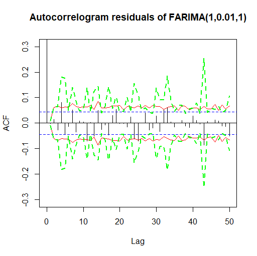
Figure 5: Autocorrelation of a realization of size $n=2,000$ for a weak FARIMA$(1,0.01,1)$ model (21)–(22) with $\theta_{0}=(0.9,0.2,0.01)$ and where $\omega=0.04$, $\alpha_{1}=0.13$ and $\beta_{1}=0.88$. The horizontal dotted lines (blue color) correspond to the 5% significant limits obtained under the strong FARIMA assumption. The solid lines (red color) and dashed lines (green color) correspond also to the 5% significant limits under the weak FARIMA assumption. The full lines correspond to the asymptotic significance limits for the residual autocorrelations obtained in Theorem 2. The dashed lines (green color) correspond to the self-normalized asymptotic significance limits for the residual autocorrelations obtained in Theorem 7.

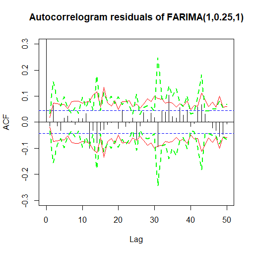
Figure 6: Autocorrelation of a realization of size $n=2,000$ for a weak FARIMA$(1,0.25,1)$ model (21)–(22) with $\theta_{0}=(0.9,0.2,0.25)$ and where $\omega=0.04$, $\alpha_{1}=0.13$ and $\beta_{1}=0.88$. The horizontal dotted lines (blue color) correspond to the 5% significant limits obtained under the strong FARIMA assumption. The solid lines (red color) and dashed lines (green color) correspond also to the 5% significant limits under the weak FARIMA assumption. The full lines correspond to the asymptotic significance limits for the residual autocorrelations obtained in Theorem 2. The dashed lines (green color) correspond to the self-normalized asymptotic significance limits for the residual autocorrelations obtained in Theorem 7.

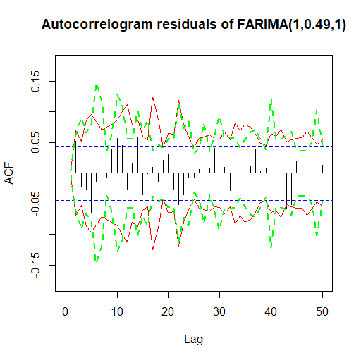
Figure 7: Autocorrelation of a realization of size $n=2,000$ for a weak FARIMA$(1,0.49,1)$ model (21)–(22) with $\theta_{0}=(0.9,0.2,0.49)$ and where $\omega=0.04$, $\alpha_{1}=0.13$ and $\beta_{1}=0.88$. The horizontal dotted lines (blue color) correspond to the 5% significant limits obtained under the strong FARIMA assumption. The solid lines (red color) and dashed lines (green color) correspond also to the 5% significant limits under the weak FARIMA assumption. The full lines correspond to the asymptotic significance limits for the residual autocorrelations obtained in Theorem 2. The dashed lines (green color) correspond to the self-normalized asymptotic significance limits for the residual autocorrelations obtained in Theorem 7.

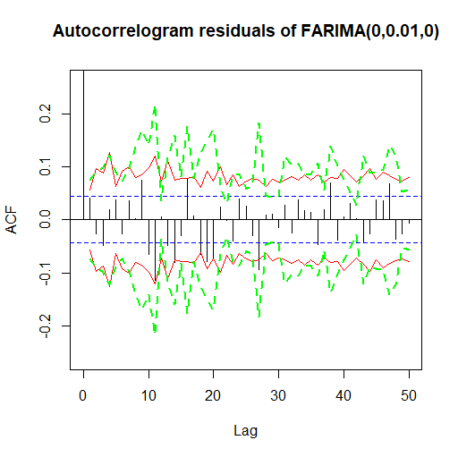
Figure 8: Autocorrelation of a realization of size $n=2,000$ for a weak FARIMA$(0,0.01,0)$ model (21)–(22) with $\theta_{0}=(0,0,0.01)$ and where $\omega=0.04$, $\alpha_{1}=0.13$ and $\beta_{1}=0.88$. The horizontal dotted lines (blue color) correspond to the 5% significant limits obtained under the strong FARIMA assumption. The solid lines (red color) and dashed lines (green color) correspond also to the 5% significant limits under the weak FARIMA assumption. The full lines correspond to the asymptotic significance limits for the residual autocorrelations obtained in Theorem 2. The dashed lines (green color) correspond to the self-normalized asymptotic significance limits for the residual autocorrelations obtained in Theorem 7.

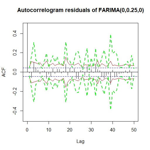
Figure 9: Autocorrelation of a realization of size $n=2,000$ for a weak FARIMA$(0,0.25,0)$ model (21)–(22) with $\theta_{0}=(0,0,0.25)$ and where $\omega=0.04$, $\alpha_{1}=0.13$ and $\beta_{1}=0.88$. The horizontal dotted lines (blue color) correspond to the 5% significant limits obtained under the strong FARIMA assumption. The solid lines (red color) and dashed lines (green color) correspond also to the 5% significant limits under the weak FARIMA assumption. The full lines correspond to the asymptotic significance limits for the residual autocorrelations obtained in Theorem 2. The dashed lines (green color) correspond to the self-normalized asymptotic significance limits for the residual autocorrelations obtained in Theorem 7.

Figure 10: Autocorrelation of a realization of size $n=2,000$ for a weak FARIMA$(0,0.49,0)$ model (21)–(22) with $\theta_{0}=(0,0,0.49)$ and where $\omega=0.04$, $\alpha_{1}=0.13$ and $\beta_{1}=0.88$. The horizontal dotted lines (blue color) correspond to the 5% significant limits obtained under the strong FARIMA assumption. The solid lines (red color) and dashed lines (green color) correspond also to the 5% significant limits under the weak FARIMA assumption. The full lines correspond to the asymptotic significance limits for the residual autocorrelations obtained in Theorem 2. The dashed lines (green color) correspond to the self-normalized asymptotic significance limits for the residual autocorrelations obtained in Theorem 7.

Contents

1. 1 Introduction
2. 2 Assumptions and estimation procedure
3. 3 Diagnostic checking in weak FARIMA models
   1. 3.1 Asymptotic distribution of the residual autocorrelations
   2. 3.2 Modified version of the portmanteau test
   3. 3.3 Self-normalized asymptotic distribution of the residual autocorrelations
4. 4 Numerical illustrations
   1. 4.1 Simulation studies and empirical sizes
   2. 4.2 Empirical power
   3. 4.3 Illustrative example
5. 5 Figures and tables
6. A Supplemental material: Proofs
   1. A.1 Preliminary results
   2. A.2 Proof of Proposition 1
   3. A.3 Proof of Theorem 2
      1. A.3.1 Step 1: Taylor’s expansion of $\sqrt{n}\hat{\gamma}_{m}$ and $\sqrt{n}\hat{\rho}_{m}$
      2. A.3.2 Step 2: asymptotic distributions of $\sqrt{n}\hat{\gamma}_{m}$ and $\sqrt{n}\hat{\rho}_{m}$
      3. A.3.3 Step 3: convergence of $R_{n,h,1}$
      4. A.3.4 Step 4: convergence of $R_{n,h,2}$
   4. A.4 Proof of Proposition 5
   5. A.5 Proof of Theorem 6
      1. A.5.1 Functional central limit theorem for $(\Lambda U_{t})_{t\geq 1}$
      2. A.5.2 Limit theorem
   6. A.6 Proof of Theorem 7
7. B Example of explicit calculation of $\Sigma_{\hat{\rho}_{m}}$ and $C_{m}$
   1. B.1 Examples of analytic and numerical computations of $\Sigma_{\hat{\rho}_{m}}$
   2. B.2 Explicit form of the matrix $C_{m}$
8. C Supplemental material: Additional Monte Carlo experiments
   1. C.1 FARIMA models with $a\neq 0$ and $b\neq 0$
   2. C.2 Small sample size
   3. C.3 GARCH process with infinite moment

References

• Akutowicz, (1957) Akutowicz, E. J. (1957). On an explicit formula in linear least squares prediction. Math. Scand., 5:261–266.
• Baillie et al., (1996) Baillie, R. T., Chung, C.-F., and Tieslau, M. A. (1996). Analysing inflation by the fractionally integrated ARFIMA-GARCH model. Journal of applied econometrics, 11(1):23–40.
• Beran et al., (2013) Beran, J., Feng, Y., Ghosh, S., and Kulik, R. (2013). Long-memory processes. Springer, Heidelberg. Probabilistic properties and statistical methods.
• Berk, (1974) Berk, K. N. (1974). Consistent autoregressive spectral estimates. Ann. Statist., 2:489–502. Collection of articles dedicated to Jerzy Neyman on his 80th birthday.
• Boubacar Mainassara et al., (2012) Boubacar Mainassara, Y., Carbon, M., and Francq, C. (2012). Computing and estimating information matrices of weak ARMA models. Comput. Statist. Data Anal., 56(2):345–361.
• Boubacar Maïnassara et al., (2019) Boubacar Maïnassara, Y., Esstafa, Y., and Saussereau, B. (2019). Estimating FARIMA models with uncorrelated but non-independent error terms. arXiv:1910.07213.
• Boubacar Maïnassara and Saussereau, (2018) Boubacar Maïnassara, Y. and Saussereau, B. (2018). Diagnostic Checking in Multivariate ARMA Models With Dependent Errors Using Normalized Residual Autocorrelations. J. Amer. Statist. Assoc., 113(524):1813–1827.
• Box and Pierce, (1970) Box, G. E. P. and Pierce, D. A. (1970). Distribution of residual autocorrelations in autoregressive-integrated moving average time series models. J. Amer. Statist. Assoc., 65:1509–1526.
• Brockwell and Davis, (1991) Brockwell, P. J. and Davis, R. A. (1991). Time series: theory and methods. Springer Series in Statistics. Springer-Verlag, New York, second edition.
• Cavaliere et al., (2017) Cavaliere, G., Nielsen, M. Ø., and Taylor, A. R. (2017). Quasi-maximum likelihood estimation and bootstrap inference in fractional time series models with heteroskedasticity of unknown form. Journal of Econometrics, 198(1):165 – 188.
• Dahlhaus, (1989) Dahlhaus, R. (1989). Efficient parameter estimation for self-similar processes. Ann. Statist., 17(4):1749–1766.
• Davidson, (1994) Davidson, J. (1994). Stochastic limit theory. Advanced Texts in Econometrics. The Clarendon Press, Oxford University Press, New York. An introduction for econometricians.
• Delgado and Velasco, (2011) Delgado, M. A. and Velasco, C. (2011). An asymptotically pivotal transform of the residuals sample autocorrelations with application to model checking. J. Amer. Statist. Assoc., 106(495):946–958.
• den Haan and Levin, (1997) den Haan, W. J. and Levin, A. T. (1997). A practitioner’s guide to robust covariance matrix estimation. In Robust inference, volume 15 of Handbook of Statist., pages 299–342. North-Holland, Amsterdam.
• Ding et al., (1993) Ding, Z., Granger, C. W., and Engle, R. F. (1993). A long memory property of stock market returns and a new model. Journal of empirical finance, 1:83–106.
• Doukhan and León, (1989) Doukhan, P. and León, J. (1989). Cumulants for stationary mixing random sequences and applications to empirical spectral density. Probab. Math. Stat, 10:11–26.
• Fan and Yao, (2008) Fan, J. and Yao, Q. (2008). Nonlinear time series: nonparametric and parametric methods. Springer Science & Business Media.
• Fox and Taqqu, (1986) Fox, R. and Taqqu, M. S. (1986). Large-sample properties of parameter estimates for strongly dependent stationary Gaussian time series. Ann. Statist., 14(2):517–532.
• Francq et al., (2005) Francq, C., Roy, R., and Zakoïan, J.-M. (2005). Diagnostic Checking in ARMA Models With Uncorrelated Errors. J. Amer. Statist. Assoc., 100(470):532–544.
• Francq and Zakoïan, (1998) Francq, C. and Zakoïan, J.-M. (1998). Estimating linear representations of nonlinear processes. J. Statist. Plann. Inference, 68(1):145–165.
• Francq and Zakoïan, (2005) Francq, C. and Zakoïan, J.-M. (2005). Recent results for linear time series models with non independent innovations. In Statistical modeling and analysis for complex data problems, volume 1 of GERAD 25th Anniv. Ser., pages 241–265. Springer, New York.
• Francq and Zakoïan, (2007) Francq, C. and Zakoïan, J.-M. (2007). HAC estimation and strong linearity testing in weak ARMA models. J. Multivariate Anal., 98(1):114–144.
• Francq and Zakoïan, (2009) Francq, C. and Zakoïan, J.-M. (2009). Bartlett’s formula for a general class of nonlinear processes. J. Time Series Anal., 30(4):449–465.
• Francq and Zakoïan, (2010) Francq, C. and Zakoïan, J.-M. (2010). GARCH Models: Structure, Statistical Inference and Financial Applications. Wiley.
• Granger and Joyeux, (1980) Granger, C. W. J. and Joyeux, R. (1980). An introduction to long-memory time series models and fractional differencing. J. Time Ser. Anal., 1(1):15–29.
• Hallin et al., (1999) Hallin, M., Taniguchi, M., Serroukh, A., and Choy, K. (1999). Local asymptotic normality for regression models with long-memory disturbance. Ann. Statist., 27(6):2054–2080.
• Herrndorf, (1984) Herrndorf, N. (1984). A functional central limit theorem for weakly dependent sequences of random variables. Ann. Probab., 12(1):141–153.
• Hong, (1996) Hong, Y. (1996). Consistent testing for serial correlation of unknown form. Econometrica, 64(4):837–864.
• Hosking, (1981) Hosking, J. R. M. (1981). Fractional differencing. Biometrika, 68(1):165–176.
• Hualde and Robinson, (2011) Hualde, J. and Robinson, P. M. (2011). Gaussian pseudo-maximum likelihood estimation of fractional time series models. Ann. Statist., 39(6):3152–3181.
• Imhof, (1961) Imhof, J. P. (1961). Computing the distribution of quadratic forms in normal variables. Biometrika, 48:419–426.
• Kuan and Lee, (2006) Kuan, C.-M. and Lee, W.-M. (2006). Robust $M$ tests without consistent estimation of the asymptotic covariance matrix. J. Amer. Statist. Assoc., 101(475):1264–1275.
• Li and McLeod, (1986) Li, W. K. and McLeod, A. I. (1986). Fractional time series modelling. Biometrika, 73(1):217–221.
• Ling, (2003) Ling, S. (2003). Adaptive estimators and tests of stationary and nonstationary short- and long-memory ARFIMA-GARCH models. J. Amer. Statist. Assoc., 98(464):955–967.
• Ling and Li, (1997) Ling, S. and Li, W. K. (1997). On fractionally integrated autoregressive moving-average time series models with conditional heteroscedasticity. J. Amer. Statist. Assoc., 92(439):1184–1194.
• Ljung and Box, (1978) Ljung, G. M. and Box, G. E. P. (1978). On a measure of lack of fit in time series models. Biometrika, 65(2):pp. 297–303.
• Lobato, (2001) Lobato, I. N. (2001). Testing that a dependent process is uncorrelated. J. Amer. Statist. Assoc., 96(455):1066–1076.
• Lobato et al., (2001) Lobato, I. N., Nankervis, J. C., and Savin, N. E. (2001). Testing for autocorrelation using a modified box- pierce q test. Inter. Econ. Review, 42(1):187–205.
• Lobato et al., (2002) Lobato, I. N., Nankervis, J. C., and Savin, N. E. (2002). Testing for zero autocorrelation in the presence of statistical dependence. Econ. Theory, 18(3):730–743.
• Magnus and Neudecker, (1999) Magnus, J. R. and Neudecker, H. (1999). Matrix differential calculus with applications in statistics and econometrics. Wiley Series in Probability and Statistics. John Wiley & Sons, Ltd., Chichester. Revised reprint of the 1988 original.
• Nielsen, (2015) Nielsen, M. Ø. (2015). Asymptotics for the conditional-sum-of-squares estimator in multivariate fractional time-series models. Journal of Time Series Analysis, 36(2):154–188.
• Palma, (2007) Palma, W. (2007). Long-memory time series. Wiley Series in Probability and Statistics. Wiley-Interscience [John Wiley & Sons], Hoboken, NJ. Theory and methods.
• Romano and Thombs, (1996) Romano, J. P. and Thombs, L. A. (1996). Inference for autocorrelations under weak assumptions. J. Amer. Statist. Assoc., 91(434):590–600.
• (44) Shao, X. (2010a). Corrigendum: A self-normalized approach to confidence interval construction in time series. J. R. Stat. Soc. Ser. B Stat. Methodol., 72(5):695–696.
• (45) Shao, X. (2010b). A self-normalized approach to confidence interval construction in time series. J. R. Stat. Soc. Ser. B Stat. Methodol., 72(3):343–366.
• Shao, (2011) Shao, X. (2011). Testing for white noise under unknown dependence and its applications to diagnostic checking for time series models. Econometric Theory, 27(2):312–343.
• Shao, (2012) Shao, X. (2012). Parametric inference in stationary time series models with dependent errors. Scand. J. Stat., 39(4):772–783.
• Shao, (2015) Shao, X. (2015). Self-normalization for time series: a review of recent developments. J. Amer. Statist. Assoc., 110(512):1797–1817.
• Tong, (1990) Tong, H. (1990). Non-linear time series: a dynamical system approach. Oxford University Press.
• Velasco and Wang, (2015) Velasco, C. and Wang, X. (2015). A joint portmanteau test for conditional mean and variance time-series models. J. Time Series Anal., 36(1):39–60.
• Wang and Sun, (2020) Wang, X. and Sun, Y. (2020). A simple asymptotically f-distributed portmanteau test for diagnostic checking of time series models with uncorrelated innovations. Journal of Business & Economic Statistics, 0(ja):1–40.
• Zhu and Li, (2015) Zhu, K. and Li, W. K. (2015). A bootstrapped spectral test for adequacy in weak ARMA models. J. Econometrics, 187(1):113–130.