The E₆ route to multicomponent dark matter

Abstract

We present a framework of dark- and visible-sector unification in the E₆ embedding of the standard model. The demand for consistently getting the standard model leads to the existence of the dark-sector. We show that the hierarchy of vevs typifying unified models leads to multicomponent dark matter at the IR. The symmetry breaking itself categorises the matter content into dark- and visible-sector particles, the categorisation being uniform across different breaking chains. We discuss the stability of the dark matter particles and compare them to existing phenomenological models of dark matter. The central results follow from symmetry and hierarchy arguments. We present an indicative set of models of gauge coupling unification, to show that the framework can be embedded in realistic models of E₆.

1 Introduction

With the building blocks of the Standard Model (SM), the particles and the interactions, all in place —their properties underpinned by experimental data [1]— it is perhaps time to look at some of the pieces of the overarching puzzle that the SM fails to put in place, and to answer some of the intriguing questions that its structure begets. The SM, in its canonical form, fails to explain neutrino oscillation data [2] and cannot account for the dark matter (DM) content of the Universe [3]. Models unifying the three interactions of the SM [4, 5] are ultraviolet (UV) safe [6, 7], renormalisable [8], and protected against quantum gravity effects [9, 10, 11], being described by a single gauged symmetry at the UV. Such frameworks predict unification of the gauge couplings and partial unification of the Yukawa couplings, giving rise to a highly predictive (albeit phenomenological) IR model. Also, unified models naturally provide the scales associated with the baryon- and lepton-number violating Weinberg operators [12] related to neutrino see-saw and proton decay. Besides, models based on $SO(10)$ and larger symmetries embed the SM fermions in anomaly free representations, providing a non-anthropic explanation for the cancellation of chiral anomalies [13, 14].

Given the evidence for particle dark matter [15, 16], an acceptable model of unification should necessarily account for the dark-sector particle content along with a mechanism for stabilising the DM particle(s). Simple groups of unification with five or more diagonal generators can provide a discrete symmetry (P_D), remnant at the IR, that stabilises the DM particle. The smallest rank-5 group of unification, $SO(10)$, embeds the fifteen SM fermions and a right-handed (RH) neutrino in the spinorial 16-dim representation. Hence, there is no place to include DM particles in the same irreducible representation (irrep). As for the scalars, all the components of any $SO(10)$ irrep, when restricted to the SM gauge symmetry $\mathcal{G}_{\mathrm{SM}}=SU(3)_{c}\times SU(2)_{w}\times U(1)_{y}$, transform similarly under the remnant P_D. Therefore, the scalars responsible for spontaneous symmetry breaking (SSB) are necessarily even to keep P_D intact. Consequently, the irreps containing the SSB scalars cannot include any DM. Thus, in order to get the dark-sector particles, one has to look for irreps in addition to the ones required to get the SM [17, 18, 19, 20, 21]. This introduces much ambiguity in model building, destroying the predictability expected from unified models.

A tidier approach would be to look for unifying frameworks which automatically generate the dark-sector while reproducing the SM. The fundamental representation of $E_{6}$, when restricted to $\mathcal{G}_{\mathrm{SM}}$, decomposes to different sub-multiplets which transform differently under P_D. Therefore, the irreps that contain the SM particles can themselves contain the dark-sector particles. When embedded in $E_{6}$, both the SM fermions and scalars transform as the 27 dimensional fundamental. The additional fermions and scalars in the fundamental irrep can then be DM candidates. Therefore, there is no arbitrariness in the choice of DM multiplets. In addition, alongside unification of the gauge symmetries, the dark- and the visible-sector particles are unified. As the DM stabilising symmetry is a remnant of the gauged $E_{6}$ itself, it is safe from Planck suppressed operators expected to break all global symmetries. Based on these observations, we study all the symmetry breaking routes of $E_{6}$ down to the SM to determine the inherent symmetry structure that simultaneously gives rise to the visible- and the dark-sector.

The results in this paper follow from the following simple demands: i) $E_{6}$ faithfully reproduces the SM, ii) the symmetry breaking from the unification scale down to the SM scale preserves the DM stabilising P_D symmetry, iii) the tiny neutrino masses are due to the see-saw mechanism, and iv) a proton decay lifetime that is safe from current bounds. We find that the hierarchy of scales in the framework leads to a DM sector that can simultaneously accommodate two different dark matter candidates. Indeed, under quite general considerations, the dark matter in $E_{6}$ is two-component, with the lightest dark-sector fermion (LDSF) and the lightest dark-sector scalar (LDSS) being DM candidates simultaneously. The lighter of the two is stable while the heavier is metastable. The metastability of the heavier DM particle is not due to any unnatural fine-tunings of the Yukawa couplings connecting the scalar and fermionic DM candidates. Instead, this is the result of the hierarchy of the scales in the unified theory. The known masses of the SM fermions determine the Yukawa couplings of the DM candidates. Also, the results do not depend on any particular route of symmetry breaking and are valid for all the maximal subgroups of $E_{6}$, namely, $SU(6)\times SU(2)$, $SO(10)\times U(1)$, and $SU(3)\times SU(3)\times SU(3)$.

Decaying and multicomponent dark matter [22, 23, 24] have been studied in the context of multiple astrophysical and cosmological observations. For example, in the context of relieving the Hubble tension [25], and in the context of the CALET and DAMPE excesses [26]. In this work, our attempt is not to present a new kind of dark matter. On the contrary, we are interested in the general structure of SSB that stabilises the DM(s) and the qualitative features of the dark-sector. In the following sections, we present our analyses. In the next section, we look at all the different ways in which the SM hypercharge can be constructed out of the diagonal generators of $E_{6}$ while preserving the non-abelian part of $\mathcal{G}_{\mathrm{SM}}$. The different definitions readily show which of them do preserve P_D at the IR and which don’t. We show that for the cases which can accommodate P_D at the IR, the particle content transforms identically under $\mathcal{G}_{\mathrm{SM}}\times U(1)_{D}\times U(1)^{\prime}$, where $U(1)_{D}$ and $U(1)^{\prime}$ are the additional ranks in $E_{6}$. It is $U(1)_{D}$ that distinguishes between the SM and the dark-sector particles. In section 3 we discuss the spectrum and the interactions of the dark-sector particles. We also show how two distinct dark matter candidates emerge in this framework. We describe the nature of the dark matter candidates, both the scalar and the fermion, and point to pre-existing analyses which study phenomenological lagrangians containing such DM candidates. In section 4, we show gauge coupling unification (GCU) for a few symmetry breaking chains to establish that our framework can easily be embedded in minimal models of $E_{6}$ unification. Finally, we conclude.

2 The E₆ fundamental and a remnant Z₂

As indicated by its name, $E_{6}$ has six diagonal generators (rank), two more than the four diagonals of the SM gauge symmetry, $\mathcal{G}_{\mathrm{SM}}\equiv SU(3)_{c}\times SU(2)_{w}\times U(1)_{y}$. The additional diagonal generators spontaneously break when scalars neutral under $\mathcal{G}_{\mathrm{SM}}$, but charged under the $U(1)$ symmetries corresponding to the said diagonals, acquire non-zero vacuum expectation values (vev). Three of the six diagonal generators of $E_{6}$ give rise to the 2+1 diagonal generators of the non-abelian part of the SM ($SU(3)_{c}\times SU(2)_{w}$), while a linear combination of the three remaining diagonals gives $U(1)_{y}$. The two orthogonal directions are broken in-between the scale of gauge coupling unification (GCU) and the scale of electroweak symmetry breaking (EWSB). Let $X=(x_{1},x_{2},x_{3})$ be the $U(1)$ charges in the basis where the hypercharge is not yet identified. To get the SM hypercharges, we perform a rotation on the $X$ basis to get the $Y=(y,y^{\prime},y^{\prime\prime})$ basis, $Y_{i}=O_{x_{i}x_{j}}X_{j}$, where $y$ is the hypercharge and $O_{x_{i}x_{j}}$ is the rotation matrix. We determine the direction of $y$ from electroweak charge assignments.

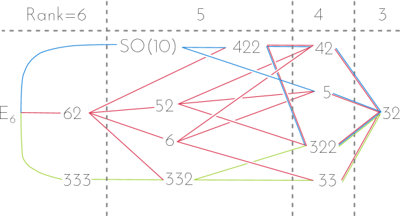
Figure 1: Symmetry breaking routes of $E_{6}$. We show only the non-abelian parts and drop the $U(1)$s. However, we indicate the number of broken generators by giving the ranks at each stage. We use a compact notation for the direct products of the $SU(N)$ symmetries, with MN representing $SU(M)\times SU(N)$.

Our goal in this section is to see which symmetry breaking routes of $E_{6}$ contain the DM-stabilising symmetry, P_D. In fig. 1, we schematically depict the different routes of breaking of $E_{6}$ down to the SM. One can build a plethora of models based on these routes by introducing different scalar multiplets to break different symmetries at different scales. In the figure, we have only shown the non-abelian symmetries, dropping the $U(1)$s for brevity. The ranks in the figure indicate the stages at which the abelian symmetries break. The presence or absence of a DM stabilising symmetry, in general, depends on the model in question. However, as we see below, without going into the details of the specific models, we can identify a few symmetry breaking chains which cannot, under any circumstance, accommodate a DM stabilising symmetry.

The cyclic group of order $N$, $Z_{N}$, is a subgroup of $U(1)\forall N$ ($Z_{1}$ being the identity). A particle that transforms non-trivially under the $U(1)$ will transform under a $Z_{N}$ symmetry after the $U(1)$ breaks spontaneously. The ‘$N$’ depends on the charge of the particle and that of the $U(1)$ breaking scalar. Let the continuous symmetry be broken at some scale $\cancel{M}$ by the non-zero vev, $\langle\phi\rangle$, of a scalar $\phi$ transforming with a charge $x_{\phi}$. Below $\cancel{M}$, $\psi$- which had a charge $x_{\psi}$ under the $U(1)$ will transform under a remnant $Z_{N}$, defined by [27, 28, 29]:

$$\psi\to\psi^{\prime}=e^{2\pi\mathrm{i}\frac{x_{\psi}}{x_{\phi}}}\psi.$$ (1)

Now, all the scalars in the spectrum that transform under the $U(1)$ and acquire a non-zero vevs break it spontaneously. The lowest SSB scale of our problem being the EWSB scale ($\cancel{M}_{\mathrm{EW}}$), the charges (if any) of the SM Higgs doublets govern the $Z_{N}$ transformation of the spectrum below $\cancel{M}_{\mathrm{EW}}$. If the charge of the Higgs is such that it breaks the symmetry to identity (following eq. 1) then, irrespective of the symmetry breaking sequence at the UV, no DM stabilising symmetry survives after $\cancel{M}_{\mathrm{EW}}$. We will use this fact along with our knowledge that the SM particle content, scalars and fermions, reside in the 27 dimensional $E_{6}$ fundamental, to separate the chains which are suitable for DM model building from the ones which are not.

The $E_{6}$ fundamental (or anti-fundamental, see appendix A), on restriction to $\mathcal{G}_{\mathrm{SM}}$, is given by:

$$27 \to(3,2,1/6)+(\overline{3},1,-2/3)+(1,1,1)+(1,2,1/2)+(3,1,-1/3)$$

$$\quad+2\times(\overline{3},1,1/3)+2\times(1,2,-1/2)+2\times(1,1,0).$$ (2)

For the case of Weyl fermions (left-handed), we immediately identify $q\equiv(3,2,1/6)$, $u^{c}\equiv(\overline{3},1,-2/3)$, and $e^{c}\equiv(1,1,1)$. We can also identify $(3,1,-1/3)$ and $(1,2,1/2)$ as BSM multiplets. There is a two-fold ambiguity regarding the down quark $d^{c}\equiv(\overline{3},1,1/3)$, the lepton doublet $\ell\equiv(1,2,-1/2)$, and the singlet neutrino $\nu^{c}\equiv(1,1,0)$. On the other hand, when the 27 contains complex scalars, we can unambiguously identify the doublet that couples to the up-type quark, $h_{u}\equiv(1,2,1/2)$. Again, there is a two-fold ambiguity regarding the identity of $h_{d}\equiv(1,2,-1/2)$. The fundamental of $E_{6}$ is a complex representation with $27$ and $\overline{27}$ transforming differently. The only $E_{6}$ invariant involving three 27 dimensional representations is $27\times 27\times 27$ (not $27\times\overline{27}\times 27$). Therefore, the doublet that gives masses to up-type quarks cannot give masses to the down-types, and we need two separate doublets, $h_{u}$ and $h_{d}$, for the up- and down-type quarks respectively. The other multiplets all represent BSM scalars.

There are three major routes for the descent of $E_{6}$ down to $\mathcal{G}_{\mathrm{SM}}$, one through $SO(10)\times U(1)$, one through $SU(6)\times SU(2)$, and another through $SU(3)\times SU(3)\times SU(3)$. These are the maximal subgroups of $E_{6}$ and these further break down to $SU(3)\times SU(2)\times U(1)^{3}$ through different intermediate symmetries, like $SU(5)$, $SU(4)\times SU(2)\times SU(2)$, $SU(3)\times SU(2)\times SU(2)$ etc., as shown in fig. 1. For each of the symmetry breaking routes, three different linear combinations of the three $U(1)$ symmetries are possible for the hypercharge. Take the $SU(3)\times SU(3)\times SU(3)$ case, for example. We identify one of the three $SU(3)$ symmetries as the $SU(3)_{c}$ of the SM. One of the two other $SU(3)$ symmetries, $SU(3)_{w}$, is broken to $SU(2)_{w}$ of the SM. A linear combination of the broken diagonal generator, $U(1)_{w}$, and both the broken diagonals of the third $SU(3)$ ($SU(3)_{N}$), gives $U(1)_{y}$ (See row 1 of table 4 for details). Two possible combinations and the corresponding orthogonal directions are ($T_{i}$ are the generators of $SU(3)$):

$$y =\frac{1}{6}T^{L}_{8}+\frac{1}{6}T^{N}_{8}\pm T^{N}_{3};\;y^{\prime}=T^{L}_{8}-T^{N}_{8};\;y^{\prime\prime}=T^{L}_{8}+T^{N}_{8}\mp\frac{1}{3}T^{N}_{3}.$$ (3)

For this definition, the restriction of the 27 to $\mathcal{G}_{\mathrm{SM}}\times U(1)_{y^{\prime}}\times U(1)_{y^{\prime\prime}}$ is:

$$27 \supset\left(3,2,\frac{1}{6}\right)(1,1)+\left(\overline{3},1,-\frac{2}{3}\right)\left(1,-\frac{5}{6}\right)+(1,1,1)\left(1,\frac{17}{6}\right)+(1,1,0)\left(1,\frac{19}{6}\right)$$

$$\quad+\left(3,1,-\frac{1}{3}\right)(-2,-2)+\left(\overline{3},1,\frac{1}{3}\right)\left(1,-\frac{7}{6}\right)+\left(\overline{3},1,\frac{1}{3}\right)(-2,2)+(1,1,0)(4,0)$$

$$\quad+\left(1,2^{*},\pm\frac{1}{2}\right)\left(-2,\mp\frac{1}{6}\right)+\left(1,2^{*},-\frac{1}{2}\right)(1,-3).$$ (4)

We identify $h_{u}\equiv(1,2^{*},1/2)(-2,-1/6)$. We have two options for $h_{d}$, $h_{d}\equiv(1,2^{*},-1/2)(-2,1/6)$ or $h_{d}\equiv(1,2^{*},-1/2)(1,-3)$. For the second identification, the $y^{\prime}$ charges of $h_{u}$ and $h_{d}$ are not equal, the former being greater than the latter. Therefore, when $h_{u}$ acquires a non-zero vev, $\langle h_{u}\rangle$, that breaks $y^{\prime}$, $h_{d}$ transforms non-trivially under the remnant $Z_{N}$, according to eq. 1. Hence, the vev of $h_{d}$, $\langle h_{d}\rangle$, breaks the $Z_{N}$. If the charge of $h_{d}$ was greater than that of $h_{u}$, then $\langle h_{u}\rangle$ would have broken any discrete remnant left by $\langle h_{d}\rangle$. On the other hand, if $h_{d}$ is identified to be $(1,2^{*},-1/2)(-2,1/6)$, then $\langle h_{d}\rangle$ does not break this $Z_{2}$. We see from section 2, there are multiplets whose $y^{\prime}$ charges are coprimes with that of $h_{u}(h_{d})$. These multiplets will transform non-trivially under the remnant $Z_{N}$ below the EW scale. For $y^{\prime\prime}$, we see that $h_{u}$ and $h_{d}$ again have equal charges. However, the charges of the other multiplets are all integer multiples of this charge. Hence, no multiplet transforms non-trivially under the $Z_{N}$ (see eq. 1). It is straightforward to see that the $Z_{N}$ remnant of $y^{\prime}$ is $Z_{2}$. In general, if the $h_{u}$, $h_{d}$ pair have non-zero $y^{\prime}$ charges then the non-zero vevs of both will keep a $Z_{N}$ unbroken iff the charges are equal. The multiplets of the spectrum below the symmetry breaking scale will transform under a remnant $Z_{N}$ if the $y^{\prime}$ charges of those multiplets are coprimes with that of $h_{u}$ and $h_{d}$. If one of the doublets is neutral under $U(1)_{y^{\prime}}$ then it plays no role in the determination of the $Z_{N}$.

With $h_{u/d}\equiv(1,2^{*},1/2)(-2,\pm 1/6)$, at $\cancel{M}_{\mathrm{EW}}$, the sub-multiplets transforms as:

$$27 \supset\left(3,2,\frac{1}{6}\right)^{-}+\left(\overline{3},1,-\frac{2}{3}\right)^{-}+\left(\overline{3},1,\frac{1}{3}\right)^{-}+(\overline{3},1,\frac{1}{3})^{+}+\left(3,1,-\frac{1}{3}\right)^{+}$$

$$+\left(1,2^{*},\pm\frac{1}{2}\right)^{+}+\left(1,2^{*},-\frac{1}{2}\right)^{-}+(1,1,1)^{-}+(1,1,0)^{+}+(1,1,0)^{-},$$ (5)

where the superscripts $+$ and $-$ denote $Z_{2}$-even and $Z_{2}$-odd respectively. The other possible definition of hypercharge in this route and the corresponding orthogonal directions are given by:

$$y =\frac{1}{6}T^{L}_{8}-\frac{1}{3}T^{N}_{8};\;y_{2}=T^{N}_{3};\;y_{3}=T^{L}_{8}+\frac{1}{2}T^{N}_{8}.$$ (6)

For this case, hypercharge is given by a linear combination of the $T_{8}^{L}$ and $T_{8}^{N}$ from $SU(3)_{L}$ and $SU(3)_{N}$ respectively, the third broken generator being a ‘spectator’. The restriction of the 27 to $\mathcal{G}_{\mathrm{SM}}\times U(1)_{y^{\prime}}\times U(1)_{y^{\prime\prime}}$ is:

$$27 \to\left(3,2,\frac{1}{6}\right)(0,1)+\left(\overline{3},1,-\frac{2}{3}\right)(0,1)+\left(3,1,-\frac{1}{3}\right)(0,-2)+(1,1,1)(0,1)+(1,1,0)\left(\pm\frac{1}{2},\frac{5}{2}\right)$$

$$\quad+\left(\overline{3},1,\frac{1}{3}\right)\left(\pm\frac{1}{2},-\frac{1}{2}\right)+\left(1,2^{*},-\frac{1}{2}\right)\left(\pm\frac{1}{2},-\frac{1}{2}\right)+\left(1,2^{*},\frac{1}{2}\right)(0,-2).$$ (7)

We immediately see that although $h_{u}$ preserves a $Z_{2}$ subgroup corresponding to $y^{\prime\prime}$, $h_{d}$, irrespective of the identification, breaks it down to identity. For $y^{\prime}$, $h_{u}$, a singlet, does not break it, while $h_{d}$ breaks it down to identity. Therefore, for this linear combination of hypercharge, a DM stabilising symmetry is not present at the IR, irrespective of the UV dynamics.

Performing the same exercise for all the symmetry breaking routes is repetitive. Hence, we push it to appendix A. In table 4, we sequentially present the decomposition of the $E_{6}$ fundamental under $SU(3)_{c}\times SU(2)_{w}\times U(1)_{x_{1}}\times U(1)_{x_{2}}\times U(1)_{x_{3}}$ for all the different symmetry breaking routes, and mention all the possible linear combinations, ($C_{1},C_{2},C_{3}$), of the $X$ charges that give the hypercharge. In table 5, we have written down the multiplets after the rotation to the $\mathcal{G}_{\mathrm{SM}}\times U(1)_{y^{\prime}}\times U(1)_{y^{\prime\prime}}$ basis. With the preceding discussion, we can use the charges in this basis to find out whether a discrete remnant of the broken $U(1)$s exist after EWSB or not, as indicated by a $\checkmark$ and a $\times$ respectively. From table 5, we see that for the cases that preserve a discrete remnant, the spectrum transforms identically under $\mathcal{G}_{\mathrm{SM}}\times U(1)_{y^{\prime}}\times U(1)_{y^{\prime\prime}}$, as given in table 1.

Fermions			$\mathcal{G}_{\mathrm{SM}}$	$U\!(1)^{\prime}$	$U\!(1)_{\mathrm{D}}$	$\mathrm{P}_{\mathrm{D}}$	Scalars
		q	$(3,2,\frac{1}{6})$	-$\frac{\kappa}{3}$	1	$-1$	$\widetilde{q}$
		$u^{c}$	$(\overline{3},1,$-$\frac{2}{3})$	$\frac{\kappa}{3}$-1	1	$-1$	$\widetilde{u}^{c}$
	Quarks	$d^{c}$	$(\overline{3},1,\frac{1}{3})$	$\frac{\kappa}{3}$+1	1	$-1$	$\widetilde{d}^{c}$	Squarks
		$\ell$	$(1,2$,-$\frac{1}{2})$	$\kappa$	1	$-1$	$\widetilde{\ell}$
		$e^{c}$	$(1,1,1)$	1-$\kappa$	1	$-1$	$\widetilde{e}^{c}$
Visible Sector	Leptons	$\nu^{c}$	$(1,0,0)$	-1-$\kappa$	1	$-1$	$\widetilde{\nu}^{c}$	Sleptons	Dark-sector
		$\widetilde{h}_{u}$	$(1,2,\frac{1}{2})$	1	-2	$1$	$h_{u}$
		$\widetilde{h}_{d}$	$(1,2,$-$\frac{1}{2})$	-1	-2	$1$	$h_{d}$
	Higgsinos	$\widetilde{s}_{4}$	$(1,1,0)$	0	4	$1$	$s_{4}$	Higgses
		$\widetilde{T}$	$(\overline{3},1$,$\frac{1}{3}$)	$\frac{2\kappa}{3}$	-2	1	$T$
Dark-sector	Hquarks	$\widetilde{T}^{c}$	$(3,1$,-$\frac{1}{3})$	-$\frac{2\kappa}{3}$	-2	1	$T^{c}$	Lquarks	Visible Sector

Table 1: We categorise the scalars and the fermions of the fundamental into visible and dark-sector particles. The multiplets which belong to the dark-sector for the fermions belong to the visible sector for the scalars, and vice-versa. We further divide the multiplets into Quarks, Leptons, Higgsinos, and Heavy Quarks for the Fermions, and Squarks, Sleptons, Higgses, and Leptoquarks for the scalars. For each of the multiplets we write down the charges under $U(1)_{D}$ and $U(1)^{\prime}$, and also the transformation under P_D. The $-1$ and the $1$ indicate $Z_{2}$ odd and even respectively.

From the seemingly arbitrary charge assignments in table 5, we obtain the simplified and consistent charge assignments as shown in table 1 from the simple considerations that the charges are defined up to a multiplicative constant and that we can perform a rotation in the $(y^{\prime},y^{\prime\prime})$ plane, keeping the SM physics the same. The multiplets have the same charges under $U(1)_{y^{\prime}}$ across the symmetry breaking routes. We identify $U(1)_{y^{\prime}}$ as $U(1)_{D}$ (‘D’ standing for dark). Under $U(1)_{D}$, all of the SM fermions have the same charge $x_{\mathrm{SM}}=1$, the dark-sector fermions have charge $x_{\mathrm{DM}}=-2$, except for the singlet which has $x_{4}=4$. With the Higgs doublets carrying a charge $1$ under $U(1)_{D}$, the SM fermions are odd and the dark-sector fermions are even after EWSB. The dark-sector fermions are chiral under $U(1)_{\mathrm{D}}$ and vector-like under $U(1)_{y^{\prime\prime}}(\equiv U(1)^{\prime})$. This forces the SM fermions (together with the RH neutrino) to cancel all the gauge and the gauge-gravity mixed anomalies among themselves for $U(1)^{\prime}$. Therefore, the $U(1)^{\prime}$ charges of the SM multiplets can be parametrised by one unknown, $\kappa$ (the charge of $\ell\equiv(1,2,-1/2)$ for our case), as shown in table 1 [30, 31]. We then use the $U(1)_{D}\times{U(1)}^{\prime 2}$ anomaly cancellation conditions to express the charges of the dark-sector vector-like triplets with that of the visible sector. The value of $\kappa$ is chain dependant. We have given the different values of $\kappa$, as obtained from table 5, in table 6. The key takeaways of this discussion are then:

1. For all the distinct routes of symmetry breaking, corresponding to the $SU(6)\times SU(2)$, the $SU(3)\times SU(3)\times SU(3)$, and the $SO(10)\times U(1)$ maximal subgroup, there is at least one chain (hypercharge definition) for which we get a DM stabilising P_D$\equiv Z_{2}$ at the IR.

2. For all the chains with P_D, the particle content transforms under $\mathcal{G}_{\mathrm{SM}}\times U(1)_{D}\times U(1)^{\prime}$ exactly the same way, as given in table 1. The dark-sector fermions are vector-like under $U(1)^{\prime}$ and hence anomaly free, forcing intra-SM anomaly cancellation. However, under $U(1)_{D}$, the dark-sector fermions are chiral. Hence, for a consistent anomaly free theory, the SM and the dark-sector particles need to cancel anomaly together, reflecting the fact that the two sectors arise from the same multiplet, i.e., dark-visible unification.

3. The situation is reversed for the scalars. The multiplets which belong to the visible-sector for the fermions belong to the dark-sector for the scalars and vice-versa.

Using these general properties of all the DM stabilising chains of $E_{6}$, we can easily categorise the particles into different sections. For the 27 of fermions, the SM particles (and the RH neutrinos) are odd under the $Z_{2}$ symmetry. The exotic fermions are all even and part of the dark-sector. As for the 27 of scalars, $h_{u}$ and $h_{d}$ are even, and the exotics include both odd and even multiplets. The scalars which are odd under the $Z_{2}$ populate a dark-sector while the even ones are part of the visible sector. To categorise all the particles of the fundamental, we ‘borrow’ nomenclature from supersymmetry, given that for each fermion there is a corresponding scalar with same quantum numbers (of course, there are three generations of fermions and only one of the scalars). There are the SM fermions, the quarks ($q,u^{c},d^{c}$) and the leptons ($\ell,e^{c},\nu^{c}$), and corresponding to them there are the ‘squarks’ ($\widetilde{q},\widetilde{u}^{c},\widetilde{d}^{c}$) and the ‘sleptons’ ($\widetilde{\ell},\widetilde{e}^{c},\widetilde{\nu}^{c}$). The squarks and the sleptons are $Z_{2}$ odd scalars populating the dark-sector, with the neutral components of the sleptons being candidates for scalar DM. Then there are the visible sector ($Z_{2}$ even) scalars, the Higgses ($h_{u},h_{d},s_{4}$), and corresponding to them, the ‘Higgsinos’($\widetilde{h}_{u},\widetilde{h}_{d},\widetilde{s}_{4}$), which are part of the dark-sector, the neutral components of which will be fermionic DM candidates. Then there are the $Z_{2}$ even scalar leptoquarks ($T,T^{c}$), and the corresponding exotic coloured fermions, which we call the heavy quarks ($\widetilde{T},\widetilde{T}^{c}$). In table 1 we list all the particles along with their labels.

Till now, we have established the $Z_{2}$ symmetry remnant after the breaking of the additional ranks of $E_{6}$. We have also derived the transformations of the particles under this $Z_{2}$. We now take a look at the possible ramifications of neutrino seesaw on this symmetry. The $\nu^{c}$ are SM singlets and we can write Majorana terms involving them. However, under the intermediate symmetries, they typically transform non-trivially. Hence, the relevant Majorana mass terms are generated from marginal Yukawa terms at the UV. Under the SM gauge symmetry, the scalar in that Yukawa will transform as a singlet, say $\delta_{R}$, and below the symmetry breaking scale at which $\delta_{R}$ gets a vev we write the relevant Majorana mass term for the $\nu^{c}$. The neutrinos also get Dirac mass from the doublet $h_{u}$. The lagrangian for the neutrino masses is:

$$\mathcal{L} \supset-y_{D}\ell h_{u}\nu^{c}-y_{M}\nu^{c}\nu^{c}\delta_{R}+\operatorname{\mathrm{h.c.}}.$$ (8)

The question then is, whether the vev of $\delta_{R}$ keeps or breaks the remnant $Z_{2}$. Let us consider the $U(1)_{D}$ symmetry that gets broken to the $Z_{2}$. For the Dirac and Majorana terms to be allowed, we must simultaneously have

$$x_{\ell}+x_{\nu^{c}}+x_{h_{u}} =0;\;2x_{\nu^{c}}+x_{\delta_{R}}=0.$$ (9)

Since the charge of $h_{u}$ preserves a remnant $Z_{2}$ under which the SM fermions are all odd, we must have $x_{\ell}=(2n+1)/2x_{h_{u}},n\in\mathbb{Z}$, implying $x_{\delta_{R}}=(2n+3)x_{u}$. Therefore, $x_{\delta_{R}}$ is an integer multiple of $x_{h_{u}}$ and hence, by eq. 1, any $Z_{2}$ that is preserved by $h_{u}$ is also preserved by the vev that gives Majorana masses to the neutrinos. Below the scale of $\langle\delta_{R}\rangle$, the lepton doublet and the Higgs doublet transforms as

$$\ell\to e^{2\pi\mathrm{i}\frac{2n+1}{2(2n+3)}}\ell;\;h_{u}\to e^{\frac{2\pi\mathrm{i}}{(2n+3)}}h_{u}.$$ (10)

After the breaking of the $U(1)$ by the seesaw scalar, the lepton and the SM Higgs are left transforming under a $Z_{2(2n+3)}$ and a $Z_{(2n+3)}$ respectively. Now, 2 and $2n+3$ are coprimes $\forall n\in\mathbb{Z}$. A cyclic group $Z_{n_{1}\times n_{2}}$ can always be decomposed to $Z_{n_{1}}\times Z_{n_{2}}$ when $n_{1}$ and $n_{2}$ are coprimes. Therefore, the lepton doublet effectively transforms under a $Z_{2}\times Z_{(2n+3)}$ while the scalar transforms under a $Z_{(2n+3)}$. The vev of the scalar then breaks the $Z_{2n+3}$ down to identity leaving the $Z_{2}$ of the lepton doublet intact. The analysis changes a little if $x_{h_{u}}=0$, but the results remain the same. We discuss such a case in appendix A.

In summary, we have categorised all the symmetry breaking chains of $E_{6}$ into those with a DM stabilising symmetry and those without one, from the basic demands of reproducing the SM. We found that for all the chains that accommodate the $Z_{2}$, the spectrum transforms in the same way. We have also shown that the vev of the scalar that gives Majorana mass to the right-handed neutrinos necessarily conserves this $Z_{2}$. There are some additional discussions on this discrete remnant of $E_{6}$ in appendix A. In the next section, we discuss the masses and the interactions of the dark-sector particles. We show that under quite general circumstances, the dark-sector can accommodate two different dark matter particles simultaneously, a real scalar and a Weyl spinor, the heavier being meta-stable.

3 E6DM, qualitatively

In the last section, we categorised the fermions and the scalars in the fundamental of $E_{6}$ into visible and dark-sector particles. We will now look at the mass hierarchies and the interactions of the particles given in table 1. With $\Psi^{I}\equiv 27_{F},(I=1(1)3)$, $\Phi\equiv 27_{S}$, $\Sigma\equiv 351^{\prime}_{S}$, the $E_{6}$ symmetric lagrangian is (check table 8 for the direct products of the 27):

$$\mathcal{L} \supset{\Psi^{I}}^{\dagger}\mathrm{i}\not{D}\Psi^{I}+D_{\mu}\Phi^{\dagger}D^{\mu}\Phi+D_{\mu}\Sigma^{\dagger}D^{\mu}\Sigma+m_{\Phi}^{2}\overline{\Phi}\Phi+m_{\Sigma}^{2}\overline{\Sigma}\Sigma-(Y_{\Phi}^{I\!J}\Psi_{I}\Psi_{\!J}\Phi+Y_{\Sigma}^{I\!J}\Psi_{I}\Psi_{\!J}\Sigma+\operatorname{\mathrm{h.c.}})$$

$$\quad-\lambda_{\Phi}(\overline{\Phi}\Phi)^{2}-\lambda_{\Sigma}(\overline{\Sigma}\Sigma)^{2}-\lambda_{\Phi\Sigma}\overline{\Phi}\Phi\overline{\Sigma}\Sigma-(\mu_{\Phi}\Phi^{3}+\mu_{\Sigma}\Phi^{2}\Sigma+\lambda^{\prime}_{\Phi\Sigma}\Phi\Phi\overline{\Sigma}\overline{\Sigma}+\operatorname{\mathrm{h.c.}}).$$ (11)

The $$\Sigma \delta_{R} \mathcal{G}_{\mathrm{SM}} Y_{\Sigma}^{I\!J}\Psi_{I}\Psi_{\!J}\Sigma I,J Y_{\Phi}^{I\!J}\Psi_{I}\Psi_{\!J}\Phi$$ multiplet contains the SM singlet (see eq. 8) that gives Majorana masses to the fermions transforming as real singlets under through the operator. To avoid unnecessary complications, we will work with a single generation of fermions and will drop the generational indices () in what follows. It is important to appreciate that the above lagrangian is what we need to write to get the SM+neutrino mass and no additional operators are present. The fermions get Dirac mass from the Yukawa operator . In terms of the SM sub-multiplets, the Yukawa lagrangian is:

$$-\mathcal{L}^{Y} =\mathcal{L}^{M}_{\Phi}+\mathcal{L}^{Y}_{\Phi}+\mathcal{L}^{M}_{\Sigma}+\mathcal{L}^{Y}_{\Sigma},$$ (12a)

$$\mathrm{where,}$$

$$\mathcal{L}^{M}_{\Sigma} =y_{\Delta}\ell\Delta_{L}\ell+y_{\delta}\nu^{c}\nu^{c}\delta_{R}+y_{8}\widetilde{s}_{4}\widetilde{s}_{4}{s}_{8}+\operatorname{\mathrm{h.c.}},$$ (12b)

$$\mathcal{L}^{M}_{\Phi} =\mathcal{L}^{M}_{SM}+\mathcal{L}^{M}_{DM},$$ (12c)

$$\mathcal{L}^{Y}_{\Phi} =\mathcal{L}^{Y}_{HQ}+\mathcal{L}^{Y}_{LQ}+\mathcal{L}^{Y}_{DM},$$ (12d)

$$\mathrm{with,}$$

$$\mathcal{L}^{M}_{SM} =y_{u}qh_{u}u^{c}+y_{d}qh_{d}d^{c}+y_{\ell}\ell h_{d}e^{c}+y_{\nu}\ell h_{u}\nu^{c}+y_{\Delta}\ell\Delta_{L}\ell+y_{\delta}\nu^{c}\nu^{c}\delta_{R}+\operatorname{\mathrm{h.c.}},$$ (12e)

$$\mathcal{L}^{M}_{DM} =y_{x}s_{4}\widetilde{h}_{u}\widetilde{h}_{d}+y_{1}\widetilde{s}_{4}\widetilde{h}_{u}{h}_{d}+y_{2}\widetilde{s}_{4}\widetilde{h}_{d}{h}_{u}+y_{c}s_{4}\widetilde{T}\widetilde{T}^{c}+\operatorname{\mathrm{h.c.}},$$ (12f)

$$\mathcal{L}^{Y}_{HQ} =(y^{\prime}_{1}d^{c}\widetilde{\nu}^{c}+y^{\prime\prime}_{1}\widetilde{d}^{c}{\nu}^{c}+y^{\prime}_{2}u^{c}\widetilde{e}^{c}+y^{\prime\prime}_{2}e^{c}\widetilde{u}^{c}+y^{\prime}_{3}q\widetilde{q})\widetilde{T}^{c}$$

$$\quad+(y^{\prime}_{4}q\widetilde{\ell}+y^{\prime\prime}_{4}\ell\widetilde{q}+y^{\prime}_{5}d^{c}\widetilde{u}^{c}+y^{\prime\prime}_{5}u^{c}\widetilde{d}^{c})\widetilde{T}+\operatorname{\mathrm{h.c.}},$$ (12g)

$$\mathcal{L}^{Y}_{LQ} =T(\widehat{y}_{3}d^{c}\nu^{c}+\widehat{y}_{4}qq+\widehat{y}_{7}\widetilde{s}_{4}\widetilde{T}+\widehat{y}_{2}u^{c}e^{c})+T^{c}(\widehat{y}_{1}q\ell+\widehat{y}_{5}u^{c}d^{c}+\widehat{y}_{6}\widetilde{s}_{4}\widetilde{T}^{c})+\operatorname{\mathrm{h.c.}},$$ (12h)

$$\mathcal{L}^{Y}_{DM} =\widetilde{h}_{u}(y_{1}\ell\widetilde{\nu}^{c}+\overline{y}_{1}\widetilde{\ell}\nu^{c}+y_{3}q\widetilde{u}^{c}+\overline{y}_{3}\widetilde{q}u^{c})+\widetilde{h}_{d}(y_{2}\ell\widetilde{e}^{c}+\overline{y}_{2}\widetilde{\ell}e^{c}+y_{4}q\widetilde{d}^{c}+\overline{y}_{4}\widetilde{q}d^{c})+\operatorname{\mathrm{h.c.}}.$$ (12i)

We have written all the terms involving the sub-multiplets in $\Phi$ and only the two terms that are relevant to fermion masses for the sub-multiplets in $\Sigma$. Note, there are some terms which are allowed by $\mathcal{G}_{\mathrm{SM}}\times Z_{2}$ at the IR but not by the unifying symmetry at the UV (check table 8 for the direct products of the irreps of $E_{6}$ and $SO(10)$). Given that Yukawa couplings are technically natural [32], they will not run to non-zero values from the zero fixed point at the $E_{6}$ breaking scale and hence, have been ignored. All the Yukawa couplings corresponding to $\Phi$ (similarly for $\Sigma$) are the low-energy manifestations of $Y_{\Phi}$. Therefore, they are all expected to be of the same order (especially, given the fact that Yukawa couplings self renormalise). In the following discussion we will use this multiple times.

In $\mathcal{L}^{M}_{\Sigma}$, we collect the terms which give Majorana masses to the fermions from the non-zero vevs of the $Z_{2}$ even singlet and triplet scalars in $\Sigma$:

$$s_{8} =\frac{v_{8}+\phi^{\prime}+\mathrm{i}a_{8}^{0}}{\sqrt{2}},\delta_{R}=\frac{v_{\mathrm{ss}}+\delta^{\prime}+\mathrm{i}a_{R}^{0}}{\sqrt{2}},\Delta_{L}=\begin{pmatrix}\delta_{L}^{+}/\sqrt{2}&\delta_{L}^{++}\\ \frac{v_{L}+\delta_{L}^{\prime}+\mathrm{i}a_{L}^{0}}{\sqrt{2}}&-\delta_{L}^{+}/\sqrt{2}\end{pmatrix}.$$ (13)

The scalars $\delta_{R},\Delta_{L}\in(126,2)_{10}/(1,6,\overline{6})_{333}/(105^{\prime},1)_{62}$ are responsible for the Majorana masses of the left- and right-handed neutrinos, as given in eq. 8, and result in a neutrino mass-matrix of:

$$M_{\nu} =\begin{pmatrix}y_{\Delta}v_{l}&y_{\nu}v_{u}\\ y_{\nu}v_{u}&y_{\delta}v_{\mathrm{ss}}\end{pmatrix},$$ (14)

where, due to the presence of both right-handed neutrinos and a triplet scalar, we have an admixture of type-I and type-II seesaw [33, 34, 35, 36]. The present uncertainty on the SM $\rho$ parameter [1] constraints $v_{l}$ to be very small, $\lesssim 1$ GeV [37], and in this work we take it to be zero. $\mathcal{L}^{M}_{\Phi}$ includes the terms which give Dirac masses to the fermions from the non-zero vevs of the $Z_{2}$ even singlet and doublet scalars in $\Phi$:

$$h_{u} =\left(h_{u}^{+},\frac{v_{u}+h_{u}^{0}+\mathrm{i}a_{u}^{0}}{\sqrt{2}}\right);\,h_{d}=\left(\frac{v_{d}+h_{d}^{0}+\mathrm{i}a_{d}^{0}}{\sqrt{2}},h_{d}^{-}\right);\,s_{4}=\frac{v_{4}+h_{4}^{0}+\mathrm{i}a_{4}^{0}}{\sqrt{2}}.$$ (15)

In $\mathcal{L}^{Y}$, we collect the terms involving scalars that do not get a vev, with $\mathcal{L}_{LQ}^{Y}$ describing interactions among the fermions and the two leptoquarks, $T$ and $T^{c}$. Models where $T$ and $T^{c}$ couple in a generation non-universal way to the SM fermions have recently gathered some attention in the context of the $R_{K^{(*)}}$ anomalies [38]. However, these leptoquarks, in general, mediate proton decay [12, 39], with the bound being $\gtrsim 10^{12}$ GeV. The leptoquarks and the squarks ($\widetilde{q},\widetilde{u}^{c}$, and $\widetilde{d}^{c}$), do not play any role in the discussions of dark matter properties and we keep them at the unification scale, following the extended survival hypothesis [40, 41].

3.1 Dark-sector Fermions and Scalars

The mass spectrum of the Higgsinos is determined by the charge assignments, the Higgsinos (and the heavy quarks) are vector-like under $U(1)^{\prime}$ and chiral under $U(1)_{D}$. Therefore, the Higgsinos get a mass at the $U(1)_{D}$ breaking scale and, are blind to $U(1)^{\prime}$ breaking. Also, $U(1)_{D}$ divides the Higgsinos into two species, with $x_{D}=-2$ and with $x_{D}=4$. Therefore, the same scalar cannot give mass to both the species. The $x_{D}=-2$ species readily get masses from $\langle s_{4}\rangle$. The SM singlet $\widetilde{s}_{4}$ remain massless when only the scalars of the fundamental and $\delta_{R},\Delta_{L}$ (eqs. 13 and 15) get non-zero vevs. There is, however, a SM singlet scalar in $\Sigma$, $s_{8}\equiv(1,1,0)(0,8),(\in(1,-8)_{101}/(1,6,\overline{6})_{333}/(15,1)_{62})$, which has a Yukawa coupling with $\widetilde{s}_{4}$, and can give it mass, as shown in eq. 12b. The mass spectrum then depends on the relative sizes of the vevs of the two $\mathcal{G}_{\mathrm{SM}}$ singlet scalars,

$$s_{4} =\frac{v_{4}+h_{4}^{0}+\mathrm{i}a_{4}^{0}}{\sqrt{2}}\in\Phi,\,s_{8}=\frac{v_{8}+\phi^{\prime}+\mathrm{i}a_{8}^{0}}{\sqrt{2}}\in\Sigma,$$ (16)

relative to $\cancel{M}_{\mathrm{EW}}$. The neutral-Higgsino mass matrix, as obtained from $\mathcal{L}^{M}_{DM}+\mathcal{L}^{M}_{SS}$ in the basis $(\tilde{s}_{4},\tilde{h}_{u}^{0},\tilde{h}_{d}^{0})$, is:

$$M_{\widetilde{h}_{0}} =\begin{pmatrix}y_{8}v_{8}&y_{1}v_{d}&y_{2}v_{u}\\ y_{1}v_{d}&0&y_{x}v_{4}\\ y_{2}v_{u}&y_{x}v_{4}&0\end{pmatrix}$$ (17)

The scalar $s_{4}$, transforming under the 27 of $E_{6}$, breaks the unifying group after acquiring a vev. Therefore, if we use it for the breaking of $E_{6}\to\mathcal{G}_{I}$, then, with $v_{d/u}\sim\cancel{M}_{\mathrm{EW}}<<v_{4}\sim\cancel{M}_{U}$, there is a hierarchical separation between the eigenvalues of the above matrix (with $v_{8}$ at a scale intermediate to the two). The diagonalising matrix, $R_{\chi}$, defined by $(\widetilde{s_{4}},\widetilde{h}_{u}^{0},\widetilde{h}_{d}^{0})^{T}=R_{\chi}(\chi_{1},\chi_{2},\chi_{3})^{T}$, $\chi_{i}$ being the diagonal basis, can be written as:

$$R_{\chi} =\frac{1}{\sqrt{2}}\begin{pmatrix}0&\sqrt{2}\cos\theta_{\chi}&-\sqrt{2}\sin\theta_{\chi}\\ 1&\sin\theta_{\chi}&\cos\theta_{\chi}\\ -1&\sin\theta_{\chi}&\cos\theta_{\chi}\\ \end{pmatrix}.$$ (18)

Defining the mass matrix in the diagonal basis as $M_{\chi}=\mathrm{diag}(M_{1},M_{2},M_{3})$, we get:

$$M_{1} =-y_{x}v_{4}\equiv-M,$$ (19a)

$$\tan 2\theta_{\chi} \simeq-2\sqrt{2}\frac{v_{u}}{v_{4}}\sim-2\sqrt{2}\frac{\cancel{M}_{\mathrm{EW}}}{\cancel{M}_{U}},$$ (19b)

$$M_{2} =y_{8}v_{8}-M\text{sec}2\theta_{\chi}\sin^{2}\theta_{\chi}\simeq y_{8}v_{8}-2M(v_{EW}/v_{U})^{2}+\mathcal{O}((v_{EW}/v_{U})^{3}),$$ (19c)

$$M_{3} =M\text{sec}2\theta_{\chi}\cos\theta_{\chi}^{2}=M(1+\mathcal{O}((v_{EW}/v_{U})^{2})).$$ (19d)

As mentioned previously, $y_{1},y_{2}$, and $y_{x}$ are all low energy manifestations of $Y_{27}$, as given in eq. 12, hence, are of the same order. Similarly, the Yukawas $y_{8}$ and $y_{\nu}$ are both low energy manifestations of the $Y_{351}$ and hence are of the same order. The scale of the seesaw vev $v_{\nu}$ is fixed by running of the couplings. Then, $y_{\nu}$ is fixed by the masses of the light neutrinos. Therefore, the order of $y_{8}$ is also fixed, making the scenario quite predictive. We can absorb the $-ve$ sign corresponding to $M_{1}$ as a phase by redefining the fermion fields.

The mixing between the doublets and the singlet, eq. 19b, is unification scale suppressed, with $\sin\theta_{\chi}\sim y_{x}\cancel{M}_{\mathrm{EW}}/\cancel{M}_{U}\simeq 10^{-20}$, where we use $y_{x}\sim 10^{-6}$ as this is the same Yukawa that suppresses the electron mass wrt $\cancel{M}_{\mathrm{EW}}$. We then have two superheavy semi-degenerate Weyl fermions, $\chi_{1}$ and $\chi_{3}$, and a third fermion $\chi_{2}\equiv\chi$ with mass $\sim y_{8}v_{8}$. In terms of the mass eigenstates, the flavour eigenstates are:

$$\tilde{s}_{4} =\cos\theta_{\chi}\chi-\sin\theta_{\chi}\chi_{3},$$ (20a)

$$\tilde{h}_{d,u} =\pm\frac{1}{\sqrt{2}}\chi_{1}+\frac{1}{\sqrt{2}}\sin\theta_{\chi}\chi+\frac{1}{\sqrt{2}}\cos\theta_{\chi}\chi_{3}.$$ (20b)

The lightest dark-sector fermion (LDSF), $\chi$, is almost entirely composed of $\tilde{s}_{4}$, while $\chi_{1}$ and $\chi_{3}$ have equal contributions from $\tilde{h}_{u}^{0}$ and $\tilde{h}_{d}^{0}$. We see from eq. 12 that all the marginal interactions of $\tilde{s}_{4}$ with the SM particles involve the $\widetilde{h}_{u,d}$. Hence, in the physical basis, are all $\sin\theta_{\chi}$ suppressed. The LDSF does have the Yukawa interactions with $\phi$, the scalar eigenstate composed predominantly of $s_{8}$. Therefore, the fermion DM candidate acts like a single Majorana DM talking to the SM through a singlet scalar. The scalar $s_{8}$ transforms as $(1,1,0)(-8,0)$ under $\mathcal{G}_{\mathrm{SM}}\times U(1)_{D}\times U(1)^{\prime}$. Therefore, its vev, and consequently the mass of $\chi$, can be kept at any scale below the intermediate symmetry breaking scale (i.e. where the gauge symmetry is $\mathcal{G}_{\mathrm{SM}}$). The mass of $\chi$ is then a quasi-free parameter of the theory.

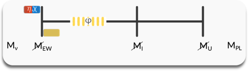
Figure 2: Hierarchy of scales in E6DM. The particles on Red backgrounds are dark-sector scalars while those on Blue backgrounds are dark-sector fermions. The ones on Yellow backgrounds are visible sector particles. In the text, we describe the masses of which particles are associated to symmetry breaking scales, which are fixed using the extended survival hypothesis, and which are (quasi-)free parameters. The scale extends from the masses of the light-neutrinos on the left to the Planck scale on the right. Between these two scales are the EWSB scale, the unification scale ($X$ and $Y$ gauge bosons), and the intermediate rank breaking (neutrino seesaw) scale. The hatched background for $\phi$, the mass eigenstate corresponding to $s_{8}$ indicates that its mass can vary over a range between the SM and the intermediate scales. The scale of $\phi$ is a parameter controlling the interaction strength between the LDSF and the SM Higgs. We describe the case where the LDSF and the LDSS are both at the EW scale. Other possibilities also exist.

The charged components of the Higgsinos get Dirac mass from the same Yukawa as their neutral counterparts and are at the same scale. The heavy quarks, $\widetilde{T},\widetilde{T}^{c}$, also get masses from the same vev as the doublet Higgsinos, as can be checked from eq. 12f. Therefore, when the vev of $s_{4}$ is at the unification scale, the charged Higgsinos and the heavy quarks are also pushed there, along with the neutral components of the doublet Higgsinos. This ensures that the heavy quarks are not the lightest dark-sector particles, protecting them from the stringent bounds from direct detection and IceCube data on strongly interacting DM particles [43, 44]. In fig. 2, we schematically depict the relevant mass scales in this framework. The visible-sector particles are on Yellow backgrounds and the dark-sector fermions are on blue backgrounds. The doublet-Higgsinos and the heavy-quarks are depicted at the unification scale, to be accurate, they are at the scale where $U(1)_{D}$ breaks. Here, in line of the discussion above, we identify it as the unification scale. In the next section, we will show a case where there is no rank breaking at the unification scale, with $U(1)_{D}$ breaking coming down to some intermediate value. The singlet Higgsino has been kept at the electroweak scale, we will discuss more about the choice in the next subsection. On Red backgrounds, we have the dark-sector scalar, the masses of which we discuss now.

The scalar potential, as given in section 3, has a global $U(1)$ preserving part and a $U(1)$ breaking part. The latter forces a mass splitting between the real and imaginary parts of the neutral dark scalars, as we show below. Also, the cubic and quartic terms involving $\Phi$ and $\Sigma$ ensure that all the visible sector scalars, except the SM Higgs, are at the scale of $v_{\mathrm{ss}}$ (the intermediate scale of neutrino seesaw) [45, 46]. Hence, at the EW scale, we only need to worry about the 125 GeV mass eigenstate. In terms of the relevant $\mathcal{G}_{\mathrm{SM}}$ sub-multiplets, the interactions of the dark-sector scalars, as given in section 3 are:

$$V_{\mathrm{DM}} =m^{2}_{\ell\ell}|\widetilde{\ell}|^{2}+m^{2}_{\nu\nu}|\widetilde{\nu}|^{2}+m^{2}_{ee}|\widetilde{\ell}|^{2}-\lambda_{\ell}|\widetilde{\ell}|^{4}-\lambda_{\nu}|\widetilde{\nu}|^{4}-\lambda_{e}|\widetilde{e}|^{4}$$

$$\quad-\lambda_{\ell\nu}\widetilde{\ell}^{\dagger}\widetilde{\ell}\widetilde{\nu}^{*}\widetilde{\nu}-\lambda_{\ell e}\widetilde{\ell}^{\dagger}\widetilde{\ell}\widetilde{e}^{*}\widetilde{e}-\lambda_{e\nu}\widetilde{e}^{*}\widetilde{e}\,\widetilde{\nu}^{*}\widetilde{\nu}$$

$$\quad-(\lambda_{u\ell}|h_{u}|^{2}+\lambda_{d\ell}|h_{d}|^{2})|\widetilde{\ell}|^{2}-\lambda_{ux}|h_{u}^{\dagger}\widetilde{\ell}|^{2}-\lambda_{dx}|h_{d}^{\dagger}\widetilde{\ell}|^{2}$$

$$\quad-(\lambda_{u\nu}|h_{u}|^{2}+\lambda_{d\nu}|h_{d}|^{2})|\tilde{\nu}|^{2}-(\lambda_{ue}|h_{u}|^{2}+\lambda_{de}|h_{d}|^{2})|\tilde{e}|^{2}$$

$$\quad-\mu_{u}h_{u}\widetilde{\ell}\widetilde{\nu}-\mu_{d}h_{d}\widetilde{\ell}\widetilde{e}-\mu_{\delta}\widetilde{\nu}\widetilde{\nu}\delta+\mathcal{O}\!\left(\frac{1}{M_{\mathrm{ss}}}\right)+\operatorname{\mathrm{h.c.}}.$$ (21)

The contributions to the scalar masses from the intermediate and the unification scales, through quartics like $\overline{\Phi}\Phi\overline{\Sigma}\Sigma$ etc., are included in the quadratic couplings, $m_{ii}$. The global $U(1)$ of the complex scalars are broken by the $\lambda_{(u/d)x}$ quartics and the $\mu_{i}$ cubics. This results in the splitting of the masses between the CP-odd and CP-even neutral scalars. The squared-mass matrix, $M^{2}_{S}$($M^{2}_{P})$, for the CP-even(odd) scalars in the flavour basis $(\widetilde{\ell}_{0}^{r},\widetilde{\nu}^{r})$ ($(\widetilde{\ell}_{0}^{i},\widetilde{\nu}^{i})$) is given by:

$$M^{2}_{S} =\frac{1}{2}\begin{pmatrix}2m^{2}_{\ell\ell}-v_{u}^{2}\lambda_{u\ell}-v_{d}^{2}(\lambda_{d\ell}+\lambda_{dx}+2\lambda_{x\ell})&\sqrt{2}v_{u}\mu_{u}\\ \sqrt{2}v_{u}\mu_{u}&2m^{2}_{\nu\nu}-v_{d}^{2}\lambda_{d\nu}-v_{u}^{2}\lambda_{u\nu}-2\sqrt{2}v_{R}\mu_{\delta}\end{pmatrix}$$ (22a)

$$M^{2}_{P} =\frac{1}{2}\begin{pmatrix}2m^{2}_{\ell\ell}-v_{u}^{2}\lambda_{u\ell}-v_{d}^{2}(\lambda_{d\ell}+\lambda_{dx}-2\lambda_{x\ell})&-\sqrt{2}v_{u}\mu_{u}\\ -\sqrt{2}v_{u}\mu_{u}&2m^{2}_{\nu\nu}-v_{d}^{2}\lambda_{d\nu}-v_{u}^{2}\lambda_{u\nu}+2\sqrt{2}v_{R}\mu_{\delta}\end{pmatrix}.$$ (22b)

The opposite signed off-diagonal elements in the two matrices are due to the difference in phase. The $U(1)$ breaking by the trilinear term corresponds to the lepton number breaking Majorana neutrino mass term in the fermion sector. The trilinear and quartic $U(1)$ breaking spurions then introduce a mass difference between the CP-even and odd scalars, as can be seen from eq. 22.

The quartic, $\lambda_{(u/d)x}$, spurions also causes mass splitting between the charged and neutral components of $\widetilde{\ell}$. However, the charged scalar masses do not have contributions from the $U(1)$ breaking trilinear, ensuring the absence of charge breaking vacua. Therefore, if all the quartics of $\Phi$ with other scalars, like $\Sigma$ and the $E_{6}$ breaking scalar, are tuned to be zero, then the charged scalars will be at the EW scale. Nevertheless, these couplings will be generated at higher orders, as quartic couplings are not self renormalising, to push the scalar masses to the intermediate or the unification scale. In general, to get scalars, dark or visible, at the EW scale we need to fine-tune the parameters of the scalar sector. Here, in accord with the extended survival hypothesis for scalars [40, 41], we keep fine-tunings at a minimum, keeping all the mass eigenstates, except for the doublet-like CP-even neutral scalar, at the seesaw scale. In that case, defining the mass basis for the CP-even scalars as,

$$\begin{pmatrix}\eta\\ \eta^{\prime}\end{pmatrix} =\begin{pmatrix}\cos\phi_{0}&\sin\phi_{0}\\ -\sin\phi_{0}&\cos\phi_{0}\end{pmatrix}\begin{pmatrix}\widetilde{\ell}_{0}^{r}\\ \widetilde{\nu}^{c}_{r}\end{pmatrix},$$ (23)

the mixing angle is given by

$$\sin 2\phi_{0} =\frac{\sqrt{2}v_{u}\mu_{u}}{M^{2}_{\eta^{\prime}}-M^{2}_{\eta}}\implies\sin\phi_{0}\simeq\frac{\sqrt{2}v_{\mathrm{EW}}\mu_{u}}{M^{2}_{\nu^{c}}}.$$ (24)

Now, $\mu_{u}$ is a remnant of the $\Phi\Phi\Sigma$ trilinear given in section 3. There is no ‘natural’ scale for the mass-dimensional coefficient of the trilinear terms. Hence, it is a free parameter of the lagrangian. In general, we see from the above relation that the mixing is intermediate scale suppressed.

The key takeaways from the scalar sector are that the CP-even scalars, the CP-odd scalars, and the charged scalar eigenvectors are not aligned and hence there is mass splitting at the tree level itself. Both the lightest CP-odd and CP-even scalar could be the DM candidate. We choose to work with the CP-even scalar as the LDSS, but the other choice is as valid. We use the mass splitting discussed above —along with the fact that quartic couplings do not self-renormalise— to keep the charged scalars and the pseudo-scalars at the scale of $v_{\mathrm{ss}}$, in a way similar to what is done for the visible sector particles [45, 46, 40, 41]. This is, in principle, the same as using the survival hypothesis to minimise fine-tuning. For these choices of the charged-scalar and the pseudo-scalar masses, the LDSS is a real-singlet at the IR. It annihilates to the SM through its couplings with the SM Higgs, as we discuss below. In fig. 2, we diagrammatically show the hierarchy in the scalar sector. The leptoquarks and the squarks are kept at the unification scale, as mentioned above. The doublet-like CP-even neutral scalar, $\eta$, is at the EW scale, while all the other sleptons are at the intermediate scale.

3.2 Decays and annihilations

The LDSF ($\chi$) and the LDSS ($\eta$) interact through extremely feeble interactions generated from the Yukawa terms in eq. 12, to be precise:

$$\mathcal{L}\supset y^{\prime}_{1}{\ell\widetilde{h}_{u}\widetilde{\nu}^{c}}+y^{\prime}_{2}{\ell\widetilde{h}_{d}\widetilde{e}^{c}}+y_{4}e^{c}\widetilde{\ell}\widetilde{h}_{d}+y_{5}\nu^{c}\widetilde{\ell}\widetilde{h}_{u},$$ (25a)

which in the mass basis is written as:

$$\mathcal{L}\supset\frac{\sin\theta_{\chi}}{\sqrt{2}}\left({y^{\prime}_{1}}\sin\phi_{0}\eta\nu+y_{5}\sin\alpha\cos\phi_{0}\nu\eta\right)\chi,$$ (25b)

where, $\sin\alpha\sim\sqrt{M_{\nu}/M_{\nu^{c}}}$ [47] is the mixing between the left- and right-handed neutrinos. Therefore, at leading order, all two-body tree-level decays of the LDSS to LDSF or vice-versa are $\sin\theta_{\chi}$, $\sin\phi_{0}$, and $y^{\prime}_{1}(y_{5})\sim y_{e}$ suppressed. Now, $\sin\theta_{\chi}\sim\frac{v_{\mathrm{EW}}}{M_{U}}$ (eq. 24) and $\sin\phi_{0}\sim\frac{v_{\mathrm{EW}}\mu_{u}}{M^{2}_{\nu^{c}}}$ (eq. 19c). This implies,

$$\Gamma\sim 2y_{e}^{2}v^{4}_{\mathrm{EW}}\frac{1}{M^{2}_{U}}\frac{\mu_{u}^{2}}{M^{4}_{\mathrm{\nu^{c}}}}M_{\eta},$$ (26)

where we choose $M_{\eta}>M_{\chi}$ (the other choice is also valid). Therefore, there is a double suppression of scales, the unification scale and the seesaw scale. Taking ‘natural’ values for the parameters in the above equation, $v_{\mathrm{EW}}\sim 10^{2}$ GeV, $y_{e}\sim 10^{-6}$, $\cancel{M}_{U}\sim 10^{16}$ GeV, $M_{\mathrm{ss}}\sim 10^{11}$ GeV, we have, $\tau_{\eta\to\chi\nu}\sim 10^{38}$ s for $\mu_{u}\sim\cancel{M}_{\mathrm{EW}}$. We have kept $M_{\eta}\sim\cancel{M}_{\mathrm{EW}}$ and have ignored the phase space factor in the above relation as it is $\lesssim 1$. This lifetime is much larger than the age of the Universe $\sim 10^{17}$s and also much larger than the bounds set on decaying dark dark matter, $\tau>10^{24}$s for $M_{\eta}\sim 100$ GeV, set by indirect observations of the neutrino spectra [48, 23]. These analyses derive the lower limit on the lifetime of the decaying dark matter particle using data on atmospheric neutrino flux as obtained from the Frejus [49], the AMANDA-II [50], and the Super-Kamiokande [51] collaborations, along with decaying dark matter searches by the IceCube collaboration [52], and also [53, 54]. We note that a $\mu_{u}$ as large as $10^{9}$ keeps the decay width above the current bound. Although we take generic values for the scales to calculate the decay width, in the next section, we will derive the scales in a few models from the demand of GCU.

Unification scale suppressed dimension-six operators leading to viable decaying dark matter candidates have been studied in the literature before [24, 23]. In such models, the decay width is suppressed by $1/\cancel{M}_{U}^{4}$. In our case, the suppression is $1/\cancel{M}_{U}^{2}$, with further suppression coming from the seesaw scale and the electron Yukawa. At this point, we note that it is crucial for the CP-even scalar coming from the doublet, $\widetilde{\ell}$, to be the LDSS. If the LDSS is dominated by $\widetilde{\nu}^{c}$, then the operator $y_{1}^{\prime}\ell\widetilde{h}_{u}\widetilde{\nu}^{c}$ will lead to $y_{1}^{\prime}\sin\theta_{\chi}\cos\phi_{0}\eta\nu/\sqrt{2}$ in the mass basis. In this case, there is no $\sin\phi_{0}$ suppression in the amplitude, and the DM lifetime will not be large enough to avoid existing bounds. The two-component DM paradigm does not work in that case.

Figure 3: On the left we show the two body decay mode of the LDSS at tree level. On the top-row at right, we show the two one-loop diagrams leading to the decay of the LDSS to a neutrino (two-body) and to a neutrino and a photon (three-body). On the right bottom-row we show the $\xi^{+}$ mediated tree-level decay to a neutrino (three-body) and to a neutrino and a photon (four-body).

The interactions of the LDSF with the charged sleptons in the mass basis, obtained from eq. 27,

$$\mathcal{L}\supset\frac{\sin\theta_{\chi}}{\sqrt{2}}\left({y^{\prime}_{2}}\sin\phi_{+}e\xi_{1}+y_{4}\cos\phi_{+}\xi_{1}^{*}e^{c}\right)\chi,$$ (27)

lead to multibody and loop-suppressed decay channels of the LDSS to the LDSF. In fig. 3, we show some of these decay modes. We immediately see that $\xi^{+}$ mediated decays to neutrinos are three-body decays at tree level and two-body decays at one-loop level. Both of these modes are suppressed by $(16\pi^{2})$ over the tree-level two-body channel. To minimise tuning, we have taken the mass difference between the LDSS and LDSF ($\Delta_{D}$) to be greater than $M_{W}$, so that the SM $W$ bosons are produced on-shell. For the case $\Delta_{D}<M_{W}$, the tree-level multi-body decay modes are further suppressed. The numerical values of the partial decay widths are dependant on the mass of the $\xi^{+}$ and hence, model dependant. However, as we have kept $\xi^{+}$ at the intermediate scale, following the survival hypothesis, the mass scale is fixed by running of gauge couplings (section 4). Therefore, in addition to the Yukawa suppression, these partial widths are suppressed by the unification scale due to the $\sin\theta_{\chi}$ in the couplings and also by $M^{4}_{\mathrm{\nu^{c}}}$, due to $\xi^{+}$ in the propagators. As a result, in comparison to the two-body tree-level decay, the one-loop decay to a neutrino and the LDSF is further suppressed by $\alpha^{2}_{\mathrm{EM}}$ and by the $16\pi^{2}$ loop-factor. The same argument holds for the three-body decay to $W$, $\nu$, and $\chi$ as well, where the loop suppression is substituted by phase-space suppression by $16\pi^{2}$. Therefore, the higher-order processes mediated by $\xi^{+}$ are also safe from the bounds discussed above.

More stringent bounds on decaying dark matter come from the observations of the isotropic gamma ray background [55, 56, 57] and the cosmic microwave background (CMB) [58]. These bounds exclude scenarios with $\tau_{\eta\to\gamma}<10^{28}$s for $M_{\eta}\sim\cancel{M}_{\mathrm{EW}}$. As we show in fig. 3, in our setup, the decay of the DM to a photon is a three-body process at one-loop and a four-body process at tree-level. Both the four-body and the one-loop three-body processes are suppressed by $\alpha^{2}_{\mathrm{EM}}/(16\pi^{2})^{2}\sim 10^{-8}$ over the tree level process. Therefore, any value of $M_{\nu^{c}}$ for which the bound from neutrinos is satisfied will automatically satisfy the bounds from the gamma ray background and the CMB. Therefore, one of the two DM candidates is absolutely stable, by virtue of the DM stabilising $Z_{2}$, P_D. The other one is metastable and is allowed by the current bounds on decaying dark matter. We have assumed the LDSS to be heavier, however, if the LDSF and the LDSS are interchanged, the conclusions remain the same as the amplitudes are the same (up to the half factor coming from averaging of incoming fermion spin). At the IR ,the DM particles act like one real-singlet scalar and one real-singlet fermion, annihilating to the SM through the Higgs boson. Such phenomenological models of DM have been extensively studied in the literature and, for the sake of completeness, we summarise some of these results.

The LDSF, $\chi$, interacts with the SM through $\cancel{M}_{U}$ and $M_{\nu^{c}}$ suppressed higher dimensional operators. However, it does have a Yukawa interaction with the singlet $s_{8}$, as given in eq. 12b. The quartic coupling of $s_{8}$ with the SM Higgs doublets introduces mass mixing between the real part of $s_{8}$, $\phi^{\prime}$ (eq. 16), and the real part of the scalars in the doublets. At leading order, this mixing is

$$\sin\beta\sim\frac{1}{y_{8}}\frac{M_{h}M_{\chi}}{M_{\phi}^{2}},$$ (28)

where $M_{\phi}$ is the mass of $\phi$, the mass eigenstate corresponding to the real part of $s_{8}$, and we have used $M_{\chi}\sim y_{8}v_{8}$ as per our derivation in eq. 19c. This mixing induces a Yukawa coupling between $\chi$ and the SM Higgs, $h$. There is also a dim-5 operator which is generated due to the $s_{8}^{*}s_{8}h^{\dagger}_{u/d}h_{u/d}$ quartics, after one $s_{8}$ has been replaced by the vev and the other has been integrated out. We parametrise the interactions as:

$$\mathcal{L} =-C^{\prime}_{\chi}\frac{v_{\mathrm{EW}}M_{\chi}}{M_{\phi}^{2}}\chi\chi h-C_{\chi}\frac{M_{\chi}}{M_{\phi}^{2}}\chi\chi hh,$$ (29)

where we have replaced $v_{8}$ with $M_{\chi}$ in the second term and absorbed the $\mathcal{O}$(1) $y_{8}$ into $C^{(\prime)}_{\chi}$. A detailed phenomenological study of singlet Majorana dark matter can be found in [59, 60, 61, 62]. From the analyses in these papers, we find that a Majorana singlet, $\chi$, with 1 GeV $\lesssim M_{\chi}\lesssim$ 1 TeV, satisfy the requirement of the thermal relic $\Omega_{c}\leq 0.12h^{2}$ ($h$ is the reduced Hubble constant) [3] for a large range of coupling strengths as calculated in the usual framework [15, 63, 16]. Global fits [64] of the parameters of the effective lagrangian, using direct-detection data from the XENON100 [65], LUX [66], XENON1T [67], and PandaX [68] collaborations, also concur (Check [69, 70] for similar models of singlet Majorana DM.).

The constraints on the trilinear coupling is much more severe than the quartic, as it leads to DM-nucleon scattering at leading order. In [71], the authors show that taking into account the measurements from the XENON1T experiment [67], the net coupling is constrained to be $\lesssim 0.01$ for $10$ GeV $<M_{\chi}<1$ TeV. For the trilinear coupling in eq. 29, this implies $M_{\phi}>1$ TeV for an $\mathcal{O}$(1) $C^{\prime}_{\chi}$ and $M_{\chi}\sim\cancel{M}_{\mathrm{EW}}$. The bounds on the coupling of the quartic are much more relaxed because it leads to DM-nucleon interactions only at one-loop, as can be seen from [64]. As an endnote to this discussion, we note that the tiny, high-scale-suppressed, couplings of the LDSF to the SM particles might also motivate a freeze-in like scenario where the LDSF is produced from the scattering of two SM particles. Freeze-In becomes particularly tempting for models where the coupling strength required to generate correct relic density via freeze-out is ruled out by current exclusions from direct detection experiments. However, at this moment we shy away from the Freeze-In mechanism for the thermal relic. As the DM and the SM particles come from the same $E_{6}$ multiplets, it is not very straightforward to understand what causes the initial abundance of the DM to be negligible as compared to that of the SM. This $\sim 0$ initial abundance of the DM particles is a necessary initial condition for the freeze-in mechanism to work. Nevertheless, some studies of singlet Majorana DM with the freeze-in mechanism can be found in [72, 73, 74].

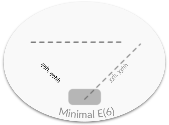
Figure 4: A schematic of the two-component DM paradigm as obtained from the fundamental of $E_{6}$, E6DM. The lightest particles of the scalar and the fermionic dark-sectors, the LDSS and the LDSF respectively, are simultaneously the DM candidates. The lighter of the two is absolutely stable, while the heavier is metastable and decays to the lighter one through unification scale and seesaw scale suppressed operators. The lifetime of the metastable DM is safe from current bounds. Both the DM particles annihilate to the SM through marginal and irrelevant couplings with the SM Higgs. The two sectors can annihilate into each other through a unification scale and seesaw scale suppressed operator, which we ignore.

The LDSS behaves as a scalar singlet dark matter [75]. The effective lagrangian (renormalisable), after EWSB, is given by

$$\mathcal{L}\supset-m_{\eta}^{2}\eta^{2}-\mu_{h}\eta^{2}h-\lambda\eta^{2}h^{2}-\lambda^{\prime}\eta^{4}.$$ (30)

The trilinear and quartic interactions of $\eta$ with the SM Higgs, $h$, are generated from the quartics between $h_{u},h_{d}$ and $\widetilde{\ell}$, as given in section 3.1. Therefore, $\eta$ either annihilates to two SM particles (including the Higgs) through the trilinear, or into two Higgses through the quartic. Detailed studies, including likelihood analyses, of such a DM particle can be found in [76, 62]. In [77], it is shown that the parameter space of a real scalar DM will be constrained by bounds from the XENON1T experiment, when the singlet contributes to all of the thermal relic. Indeed, in [71] the data from XENON1T have been taken into account to show that the bound on the trilinear is as strong as $<0.001$ for 10 GeV $<M_{\eta}<$ 100 GeV. Lastly, in our case of minimal fine-tuning, where only a CP-even scalar singlet is light at the electroweak scales, the CP-odd partner is kept at a scale much higher than the mass of $\eta$. Hence, the vector boson mediated neutral current interaction with nucleons are essentially zero. However, the mass splitting need not be orders of magnitude. A splitting $\sim 100$ keV is enough to suppress DM-nucleon couplings to an extent that makes it safe from direct-detection constraints [78]. Therefore, models where the pseudoscalar is at the EW scale are also viable.

The above discussion on the nature of the stable and metastable DM candidates as obtained from the $E_{6}$ fundamental, along with the discussion in section 2 on the symmetry strcture of the $E_{6}$ fundamental on restriction to $\mathcal{G}_{\mathrm{SM}}\times Z_{2}$ brings an end to our main points of interest. In fig. 4, we describe the framework, labelled E6DM, diagrammatically. In short, we describe a scenario of visible- and dark-sector unification, where a scalar DM sector, a fermion DM sector, and the SM (+ an RH neutrino) come from the same UV multiplet, three copies of which contain the three generations of the SM fermions and a single copy contains the EW breaking scalar. The lighter of the lightest dark-sector scalar (LDSS) and the lightest dark-sector fermion (LDSF) is absolutely stable, the heavier being metastable but with a lifetime allowed by all current bounds on decaying dark matter. The decay of the heavier DM particle to the lighter is unification scale, seesaw scale, and the electron Yukawa suppressed. The LDSS and the LDSF both annihilate to the SM through a Higgs portal. We have ignored the annihilation of the dark matter particles into each other. The most interesting point is that this framework only uses the multiplets required to get the SM from $E_{6}$ and do not introduce additional multiplets. In the next section, we analyse the running of gauge couplings for a few representative symmetry breaking chains to show that the above paradigm can easily be embedded in minimal $E_{6}$ models for the most constrained case of one intermediate scale between $\cancel{M}_{U}$ and $\cancel{M}_{\mathrm{EW}}$ while satisfying the bounds set by proton-decay experiments and also while reproducing the correct light neutrino mass.

4 Symmetry breaking chains

Having described all the moving parts that go into the E6DM paradigm, we look at the running of gauge couplings to establish that the hierarchy of masses that leads to the key results, as described above, can be embedded in a consistent model of gauge coupling unification (GCU). We stick to the minimal case of one scale, $\cancel{M}_{I}$, intermediate to the unification scale, $\cancel{M}_{U}$, and the electroweak scale, $\cancel{M}_{\mathrm{EW}}$. This is the most stringent case, as adding more intermediate scales allows for more leeway to tune the parameters. To make our study representative, we look at one case each from the three routes given in fig. 1, the $SU(3)\times SU(3)\times SU(3)$ route, the $SO(10)\times U(1)$ route, and the $SU(6)\times SU(2)$ route. As for scalar multiplets, we do not use multiplets with dimensionality larger than 351 in any way. As a result, we do not look at chains that require the extremely large 650 or 1728 dimensional multiplets often used in $E_{6}$ model building. The three chains we look at are:

$$\mathrm{I}\quad E_{6}\xrightarrow[M_{U}]{(15,1)_{62}\subset 351^{\prime}}422\xrightarrow[M_{I}]{(10,1,3)_{422}\subset 351^{\prime}}\mathcal{G}_{\mathrm{SM}}\xrightarrow[M_{Z}]{(1,2,\pm\frac{1}{2})_{\mathcal{G}_{\mathrm{SM}}}\subset 27}\mathcal{G}_{\cancel{\mathrm{SM}}},$$ (31a)

$$\mathrm{II}\quad E_{6}\xrightarrow[M_{U}]{45(4)_{101}\subset 351}3221\xrightarrow[M_{I}]{(1,1,3)(-2)_{3221}\subset 351^{\prime}}\mathcal{G}_{\mathrm{SM}}\xrightarrow[M_{Z}]{(1,2,\pm\frac{1}{2})_{\mathcal{G}_{\mathrm{SM}}}\subset 27}\mathcal{G}_{\cancel{\mathrm{SM}}},$$ (31b)

$$\mathrm{III}\quad E_{6}\xrightarrow[M_{U}]{(1,1,8)_{333}\subset 78}3321\xrightarrow[M_{I}]{(1,6,3)(-\frac{2}{3})_{3321}\subset 351^{\prime}}\mathcal{G}_{\mathrm{SM}}\xrightarrow[M_{Z}]{(1,2,\pm\frac{1}{2})_{\mathcal{G}_{\mathrm{SM}}}\subset 27}\mathcal{G}_{\cancel{\mathrm{SM}}}.$$ (31c)

The first chain belongs to the $SU(6)\times SU(2)$ route of $E_{6}$ breaking. This route is minimal in the sense that only the scalars required for giving masses to the SM fermions are used for the symmetry breaking of $E_{6}$ down to the SM. The sub-multiplet transforming as $(15,1)$ under $SU(6)\times SU(2)$, residing in the $351^{\prime}$, breaks $E_{6}$ down to the intermediate $SU(4)\times SU(2)\times SU(2)$ symmetry and simultaneously gives mass to $\widetilde{h}_{u/d}$ at the unification scale, resulting in the hierarchy of masses between the doublet Higgsinos and the singlet Higgsino, as described in section 3.1. The $\widetilde{h}_{u/d}$ reside in the $(\overline{6},2)$, with $(\overline{6},2)\times(\overline{6},2)\times(15,1)$ being a gauge singlet. For this chain, the unification scale is $1.3\times 10^{16}$ GeV and the unified coupling strength is 0.55, resulting in a proton decay lifetime of $2.5\times 10^{36}$ years, that is allowed by current limits on the same from the Super-Kamiokande experiment, setting the exclusions lower limit at $\tau_{p}>1.6\times 10^{34}$ yrs [79]. The intermediate scale is at $1.4\times 10^{11}$ GeV where $SU(4)\times SU(2)\times SU(2)$ breaks to $\mathcal{G}_{\mathrm{SM}}$, giving masses to the RH neutrinos. We discuss the details of the running of gauge couplings and the proton lifetime calculations below. Here, we note that both the unification scale and the intermediate is amenable to the paradigm of E6DM. Indeed, $\cancel{M}_{I}\sim 10^{11}$ GeV and $\cancel{M}_{U}\sim 10^{16}$ GeV are the ‘generic’ values that we used in the last section to get our results. Rank breaking takes place in two steps. First, at the unification scale, $U(1)_{D}$ breaks to give mass to the doublet Higgsinos, and the second is at the intermediate scale where the RH neutrinos get mass.

ID	Chain	$M_{I}$ (GeV)	$M_{U}$ (GeV)	$g_{U}$	$\tau_{p\to\pi^{0}e^{+}}$ yrs
I	$4_{C}2_{L}2_{R}$	$1.4\times 10^{11}$	$1.3\times 10^{16}$	0.55	$2.5\times 10^{36}$
II	$3_{C}2_{L}2_{R}1_{BL}$	$3.1\times 10^{9}$	$1.2\times 10^{16}$	0.54	$1.9\times 10^{36}$
III	$3_{C}3_{L}2_{N}1_{N}$	$5.6\times 10^{6}$	$4.9\times 10^{15}$	0.60	$3.6\times 10^{34}$

Table 2: We write down the values of the intermediate and $E_{6}$ symmetry breaking scales for each of the chains in consideration. We mention the value of the unified coupling constant, $g_{U}$. The last column shows the proton decay lifetime ($p\to\pi^{0}e^{+}$) as calculated using $\cancel{M}_{U}$ and $g_{U}$.

The second chain belongs to the $SO(10)\times U(1)$ route and is similar to the one discussed above. The unified symmetry is broken by the $(45)(4)_{101}$ sub-multiplet of $SO(10)\times U(1)$ that resides in the $351$ of $E_{6}$. The intermediate symmetry is broken to $\mathcal{G}_{\mathrm{SM}}$ by the $(1,1,3)(-2)_{3221}$ sub-multiplet residing in the $351^{\prime}$ of $E_{6}$ at a scale of $3.1\times 10^{9}$ GeV. This is the scale of RH neutrino mass. As can be checked from our order of magnitude arguments in section 3.2, an intermediate scale around $10^{9}$ GeV, although lower than the generic $10^{11}$ GeV that we used, is still high enough for all the conclusions to remain valid. The doublet Higgsinos get masses from the vev of the $E_{6}$ breaking scalar (the mass term being the $(10,-2)^{F}_{101}\times(10,-2)^{F}_{101}\times(45,4)^{S}_{101}$ singlet). Therefore, they remain heavy at the unification scale, as required by E6DM. Although, the $U(1)_{D}$ breaking scalar, $s_{4}$, resides in the fundamental itself, we also get it from other multiplets that break the unification symmetry. For the first chain it was the $(15,1)_{62}$, whereas for this one, it is the $(45,4)_{101}\subset 351$. This ensures that there isn’t a huge hierarchy of vevs among the different directions of the fundamental. As a side note, the $SU(4)\times SU(2)\times SU(2)$ is a subgroup of both $SO(10)\times U(1)$ and $SU(6)\times SU(2)$. The reason we associate the $422$ chain with $SU(6)\times SU(2)$ and not $SO(10)\times U(1)$ is because of the $L\leftrightarrow R\,Z_{2}$ subgroup of $SO(10)$, commonly referred to as $D$-parity [80]. We checked that the one-step unification with $422D$ gives an $\cancel{M}_{U}$ that is too low to pass proton decay exclusions. $E_{6}$ is broken to $422$ through the $SO(10)$ route by the $(54)(4)_{101}\subset 351^{\prime}$ which preserves $D$-parity. To break $E_{6}$ to $422$ without D-parity, one needs to resort to the 650 dimensional representation that contains the 210-dim $SO(10)$ representation. As discussed above, we do not look at scalars in multiplets which are larger than 351 dimensional.

The third chain is pathological in multiple ways and we will use it to underline a few key points. First of all, the intermediate scale is too low, $\sim 10^{6}$ GeV, for providing enough suppression to the operators that make the heavier DM particle to decay to the lighter one. However, what is much more pressing is that both the additional ranks are broken at this intermediate scale. This implies that the doublet Higgsinos also get a mass at this scale. Since the first generation of the Higgsinos get a Yukawa suppression that is the same as electron Yukawas, there mass comes at around 1-10 GeV. Therefore, even from the point of view of single component dark matter, this chain is pathological. As discussed above, the Higgsinos can only get a mass at the scale where $U(1)_{D}$ breaks. Therefore, for the E6DM paradigm to work, $U(1)_{D}$ should break close to $\cancel{M}_{U}$, if not equal to it. It is important to note that not all SSBs break rank. The DM sector given by minimal $E_{6}$ is a result of the symmetry group itself. The two-component scenario arises when we choose a specific hierarchy between vevs. Check [81], for a study of single-component fermionic DM arising from the $SO(10)$ chain of $E_{6}$.

One- and two-loop $\beta$-coefficients for $\mathcal{G}_{\mathrm{SM}}\equiv SU(3)_{c}\times SU(2)_{w}\times U(1)_{y}$
$n_{g}=2$	$n_{g}=1$	$n_{g}=0$
$\begin{pmatrix}-\frac{17}{3}\\ -\frac{11}{6}\\ \frac{163}{30}\end{pmatrix}\begin{pmatrix}-\frac{2}{3}&\frac{9}{2}&\frac{41}{30}\\ 12&\frac{133}{6}&\frac{3}{2}\\ \frac{164}{15}&\frac{9}{2}&\frac{667}{150}\end{pmatrix}$	$\begin{pmatrix}-\frac{19}{3}\\ -\frac{5}{2}\\ \frac{143}{30}\end{pmatrix}\begin{pmatrix}-\frac{40}{3}&\frac{9}{2}&\frac{37}{30}\\ 12&14&\frac{6}{5}\\ \frac{148}{15}&\frac{18}{5}&\frac{316}{75}\end{pmatrix}$	$\begin{pmatrix}\frac{41}{10}\\ -\frac{19}{6}\\ -7\end{pmatrix}\begin{pmatrix}\frac{199}{50}&\frac{27}{10}&\frac{44}{5}\\ \frac{9}{10}&\frac{35}{6}&12\\ \frac{11}{10}&\frac{9}{2}&-26\end{pmatrix}$

(a) One- and two-loop $\beta$ coefficients for the three couplings of the $\mathcal{G}_{\mathrm{SM}}$ symmetry.

Chain	Symmetry	One- and two-loop $\beta$-coefficients
		$n_{g}=2$	$n_{g}=1$
I	$422$	$\begin{pmatrix}-\frac{17}{3}\\ -1\\ \frac{17}{3}\end{pmatrix},\begin{pmatrix}\frac{985}{6}&\frac{15}{2}&\frac{159}{2}\\ \frac{75}{2}&33&6\\ \frac{795}{2}&6&\frac{659}{3}\end{pmatrix}$	$\begin{pmatrix}-\frac{19}{3}\\ -\frac{5}{3}\\ 5\end{pmatrix},\begin{pmatrix}\frac{875}{6}&\frac{15}{2}&\frac{159}{2}\\ \frac{75}{2}&\frac{149}{6}&\frac{9}{2}\\ \frac{795}{2}&\frac{9}{2}&\frac{423}{2}\end{pmatrix}$
II	$3221$	$\begin{pmatrix}-\frac{17}{3}\\ -\frac{3}{2}\\ -\frac{5}{6}\\ \frac{22}{3}\end{pmatrix},\begin{pmatrix}-\frac{2}{3}&\frac{9}{2}&\frac{9}{2}&\frac{7}{6}\\ 12&\frac{53}{2}&6&\frac{9}{4}\\ 12&6&\frac{271}{6}&\frac{57}{4}\\ \frac{28}{3}&\frac{27}{4}&\frac{171}{4}&\frac{401}{12}\end{pmatrix}$	$\begin{pmatrix}-\frac{19}{3}\\ -\frac{13}{6}\\ -\frac{3}{2}\\ \frac{20}{3}\end{pmatrix},\begin{pmatrix}-\frac{40}{3}&\frac{9}{2}&\frac{9}{2}&\frac{5}{6}\\ 12&\frac{55}{3}&\frac{9}{2}&\frac{9}{4}\\ 12&\frac{9}{2}&37&\frac{57}{4}\\ \frac{20}{3}&\frac{27}{4}&\frac{171}{4}&\frac{397}{12}\end{pmatrix}$
III	$3321$	$\begin{pmatrix}-5\\ -\frac{7}{6}\\ \frac{19}{6}\\ \frac{67}{6}\end{pmatrix},\begin{pmatrix}12&12&\frac{9}{2}&\frac{3}{2}\\ 12&\frac{529}{3}&\frac{135}{2}&\frac{155}{6}\\ 12&180&\frac{440}{3}&18\\ 12&\frac{620}{3}&54&\frac{170}{3}\end{pmatrix}$	– N/A –

(b) One- and two-loop $\beta$ coefficients for the different intermediate symmetries for different cardinalities of the Higgsinos and the heavy quarks.

Table 3: One- and two-loop $\beta$-coefficients corresponding to the different gauge couplings. The two-loop coefficients are calculated using the techniques in [82, 83]. The column matrices give the one-loop coefficients and the $2\times 2$ matrices give the two-loop coefficients. The ordering of the coefficients follow the ordering of the symmetries in their naming. For example, for $\mathcal{G}_{\mathrm{SM}}$, $SU(3)_{c}$ is followed by $SU(2)_{w}$ followed by $U(1)_{y}$. The quantity $n_{g}$ gives the number of generations of the Higgsinos and the Heavy Quarks that contribute to the running at that stage.

To get the scales and the couplings, as shown in table 2, we calculate the running of the gauge couplings using two-loop $\beta$-coefficients, following the method outlined in [84, 85, 86]. The $\beta$-coefficients corresponding to the different symmetry groups and the different stages of running are given in table 3. For the first two chains, all three generations of the doublet Higgsinos and the heavy quarks get mass from the $E_{6}$ breaking vev. The masses of the three different generations are Yukawa suppressed, the Yukawa couplings being commensurate with the Yukawa couplings of the three generations of the SM fermions, as discussed in section 3.1. Accordingly, we keep the third generation at the unification scale itself, the second generation is integrated out at $10^{-3}\times\cancel{M}_{U}$ and the first generation at $10^{-6}\times\cancel{M}_{U}$. There will be slight differences in the Yukawas due to running (of these Yukawa couplings), but we have checked that small changes to the masses of these fermions do not modify the resulting scales in any significant way. As the mass of the first generation (lightest) is close (within an order of magnitude) to the intermediate scale for the first two chains, we do not introduce its mass as a different scale, but as threshold corrections [87, 88] corresponding to the intermediate scale. Therefore, between the unification and the intermediate scale, there is another scale at $10^{-3}M_{U}$, obtained by integrating out the second generation of the doublet Higgsinos and the heavy quarks. The third generation is kept at the unification scale and the first generation is introduced as threshold correction to the intermediate scale. In table 3(b), we separately show the $\beta$-coefficients corresponding to the intermediate symmetries where the cardinality ($n_{g}$) of the dark-fermion generations is two and where it is one. The matching at the intermediate scale for the couplings are given by:

$$\mathrm{(I)}\; w_{c}=w_{4}-\frac{1}{3\pi}-\mathcal{R}_{\mathrm{T}};\;w_{w}=w_{2}-\mathcal{R}_{\mathrm{T}};\;w_{y}=\frac{3}{5}w_{2N}+\frac{2}{5}w_{4}-\frac{7}{30\pi}-\mathcal{R}_{\mathrm{T}},$$ (32a)

(II) $$w_{c}=w_{3}-\mathcal{R}_{\mathrm{T}};\;w_{w}=w_{2}-\mathcal{R}_{\mathrm{T}};\;w_{y}=\frac{3}{5}w_{R}+\frac{2}{5}w_{BL}-\frac{1}{6\pi}-\mathcal{R}_{\mathrm{T}},$$ (32b)

(III) $$w_{c}=w_{c};\;w_{w}=w_{3W}-\frac{1}{12\pi};\;w_{y}=\frac{3}{5}w_{2N}+\frac{1}{5}w_{N}+\frac{1}{5}w_{3W}-\frac{3}{20\pi},$$ (32c)

$$\mathrm{with},\, w_{i}=\frac{g_{i}^{2}}{4\pi};\;\mathcal{R}_{\mathrm{T}}=\frac{1}{3\pi}\left(\ln\frac{M_{U}}{M_{I}}-6\ln 10\right).$$ (32d)

The quantity $\mathcal{R}_{\mathrm{T}}$ is the threshold correction as discussed above. For the first two chains, only the singlet dark matter particles and the singlet scalar $\phi$ (the mass eigenstate of $s_{8}$) remain propagating degrees of freedom on top of the SM particles (as the sleptons are kept heavy at the intermediate scale, section 3.1) below the intermediate scale. As gauge singlets do not contribute to $\beta$-coefficients of the gauge couplings, the $\mathcal{G}_{\mathrm{SM}}$ running of couplings for the first two chains are the same as the SM case, as can be seen from column 3 of table 3(a). For the disallowed chain III, all three generations contribute to running between $\mathcal{M}_{U}$ and $\mathcal{M_{I}}$. The Higgsinos and the heavy quarks are integrated out in the SM stage of running and hence we show the $\beta$ coefficients of the SM symmetry for the two stages corresponding to 2 generations and 1 generation of the exotic fermions propagating ($n_{g}=2$ and $1$ respectively) in table 3(a). The hierarchy of the masses for the first two chains (i.e. the allowed chains) is schematically shown in fig. 2.

In non-supersymmetric models of unification, gauge boson induced dim-6 operators are the leading contributors to proton decay. These operators are: [89, 90, 45]:

$$\mathcal{O}_{L}\left(e^{c},d\right) =\frac{g_{U}^{2}}{2M_{U}^{2}}\left[1+|V_{ud}|^{2}\right]\;\epsilon^{ijk}\overline{u^{c}_{i}}\gamma^{\mu}u_{j}\overline{e^{c}}\gamma_{\mu}d_{k},$$ (33a)

$$\mathcal{O}_{R}\left(e,d^{c}\right) =\frac{g_{U}^{2}}{2M_{U}^{2}}\left[1+|V_{ud}|^{2}\right]\;\epsilon^{ijk}\overline{u^{c}_{i}}\gamma^{\mu}u_{j}\overline{d^{c}_{k}}\gamma_{\mu}e,$$ (33b)

where $|V_{ud}|=0.9742$ is the CKM matrix element [1] between up and down quarks. The partial width for the channel $p\to\pi^{0}e^{+}$ is expressed as [45, 89]:

$$\frac{1}{\tau_{p}} =\frac{m_{p}}{32\pi}\left(1-\frac{m_{\pi^{0}}^{2}}{m_{p}^{2}}\right)^{2}R_{L}^{2}\frac{g_{U}^{4}}{4\cancel{M}_{U}^{4}}(1+|V_{ud}|^{2})^{2}\left(R_{SR}^{2}|\langle\pi^{0}\rvert(ud)_{R}u_{L}\lvert p\rangle|^{2}+R\to L\right),$$ (34)

where $m_{p}$=938.3 MeV and $m_{\pi^{0}}$= 134.98 MeV are the masses of proton and the neutral pion respectively [1]. $R_{L}\simeq 1.33$ [91] is the long-range renormalisation factor for the proton decay operator from the electroweak scale to the QCD scale ($\sim 1$ GeV), whereas, $R_{SR(L)}$ is the short-range enhancement factor arising due the renormalisation group evolution of the proton decay operator $\mathcal{O}_{R(L)}$ from the unification to the electroweak scale. The short-range enhancement factors depend on the breaking chains. However, we use a conservative value, $R_{SR}=R_{SL}=2.4$ [92, 93]. The form-factors as provided by the lattice QCD computation are [94]:

$$\langle\pi^{0}\rvert(ud)_{R}u_{L}\lvert p\rangle=-0.131,\ \ \langle\pi^{0}\rvert(ud)_{L}u_{L}\lvert p\rangle=0.134\ .$$ (35)

In summary, we have shown that the hierarchy of masses and scales as required by the E6DM paradigm can be achieved easily in models of unification, using a few representative chains of GCU. We have also used a chain where the paradigm does not work to establish the relation between the masses of the exotic fermions and rank breaking of $E_{6}$. We have calculated the proton decay lifetime for the chains under consideration to show that they are allowed by current exclusions. The hierarchy of masses of the scalars are not protected against radiative corrections, like all non-supersymmetric models with multiple stages of symmetry breaking. However, the models can be supersymmetrised to stabilise the masses. Our results are all based on the gauge symmetry under question and will not interfere with global supersymmetry. We have intentionally restricted ourselves to the minimal case of one intermediate symmetry and to small scalar multiplets as these are the cases with least freedom of playing around with parameters. Therefore, the results shown here should easily be reproduced in non-minimal models with more symmetry breaking scales and larger scalar multiplets.

5 Conclusion

We discuss a framework for dark- and visible-sector unification with the SM embedded in $E_{6}$. The copies of the $E_{6}$ fundamental containing the SM include the dark-sector as well. The framework accommodates multicomponent dark matter, one scalar and one fermionic, under quite general circumstances. The lighter of the two is stable, while the heavier is metastable with a lifetime allowed by current exclusions. The stability of the heavier component is not due to any unnatural fine-tuning of the parameters. It is ensured by the $E_{6}$ symmetry and the hierarchy of vevs. The framework is not partial to any specific symmetry breaking route of $E_{6}$. As we discussed a non-SUSY version of $E_{6}$, the hierarchical separation between the scalars is not guaranteed to be preserved by radiative corrections. The simplest solution to this is to supersymmetrise the model [95, 96]. Our results follow from the gauge symmetry and will not be modified for a SUSY version. The calculations for the running of couplings, however, would need to be modified.

We do not add multiplets additional to those required for the SM, also, the symmetry at the UV is just $E_{6}$, not compounded with any other symmetries, gauged or otherwise. We discuss, in detail, the different ways in which the SM hypercharge is obtained from a linear combination of the three additional ranks of $E_{6}$ (ones in addition to the non-abelian part of the SM). We show that from this definition of hypercharge we can separate the chains that can give rise to a DM stabilising $Z_{2}$ symmetry at the IR from the ones that can’t. For the definitions that preserve this discrete symmetry, the particle content (SM+exotics) transforms identically under the $SU(3)_{c}\times SU(2)_{w}\times U(1)_{y}\times U(1)_{D}\times U(1)^{\prime}$, irrespective of intermediate symmetry breaking. Here, $U(1)_{D}$ and $U(1)^{\prime}$ are the $U(1)$ symmetries corresponding to the additional ranks of $E_{6}$. It is $U(1)_{D}$ that differentiates the SM particles from the dark-sector particles, and its discrete remnant stabilises the DM particles at the IR.

The scalar DM resides in the multiplet that contains the EW breaking Higgs doublets, and the fermionic DM comes from the multiplets containing the SM fermions. The fermions being embedded in the anomaly free fundamental of $E_{6}$, the question of anomaly cancellation does not arise. Yet, what is notable is that there is intra-SM anomaly cancellation for the $U(1)^{\prime}$ that doesn’t stabilise the DM and there is SM-DM mixed anomaly cancellation for the DM stabilising $U(1)_{D}$. The interactions between the lightest particles of the fermionic, and the scalar sectors are all suppressed by the unification scale, the seesaw scale and the electron Yukawa simultaneously. The resulting decay width is large enough to give a lifetime that is much larger than the age of the Universe and allowed by existing bounds on decaying dark matter. To get this stability, we do not need to introduce any fine-tuning in the framework on top of the generic tunings present in the scalar sector of unified models, namely the survival hypothesis. The hierarchy that guarantees the metastability of the heavier DM particle is, however, a choice. It is possible to build models with a different choice of scales where only the lightest particle is a DM candidate, dictated by the stabilising remnant of $U(1)_{D}$.

At the IR, both the scalar and the fermionic DM particles annihilate to the SM through the Higgs portal. The fermionic DM talking to the Higgs through the Yukawa coupling that gives it mass. Our interest was in the qualitative features of this two-component DM sector. We have discussed the thresholds that go into the spectrum, mentioning the different symmetry breaking scales which determine the masses of the exotics. We can extend this general framework to build various models with diverse IR phenomenology. We look at the two stable DM candidates individually, but a proper study of the cosmological evolution, including the interplay of the two different DM candidates, is an interesting prospect. However, as the couplings of the DM particles to each other are all high-scale suppressed, it is a good approximation to treat them separately. Also, any proper phenomenological study based on a Unified framework must include a multi-parameter fit involving observed values of the fermion masses, low energy observables, and running of the scalar and Yukawa couplings leading to unification. That was certainly not our goal, and we leave this exercise for future endeavours. Here, as proof of principle, we study the unification of gauge couplings for the three maximal subgroups of $E_{6}$. As seen from this exercise, we can easily embed the framework in a minimal model of gauge coupling unification. We also describe a ‘null’ case where the setup breaks down.

Acknowledgements: The authors thank Avik Banerjee and Joydeep Chakrabortty for useful discussions and also for giving the final manuscript a thorough read. TB acknowledges the Workshop on High Energy Physics Phenomenology (WHEPP) 2017 for providing a platform for discussions that eventually led to this work. TB also thanks Joydeep Chakrabortty for hosting him at IIT Kanpur, India for two weeks in March 2018 where this work commenced. RM acknowledges a UGC-NET fellowship.

Appendix A P_D for all the E₆ chains

In this appendix, we explicitly show the decomposition of the $E_{6}$ fundamental under the different intermediate symmetries. As discussed in the main text, there are three distinct maximal subgroups of $E_{6}$ —$SU(3)\times SU(3)_{L}\times SU(3)_{N}$, $SO(10)\times U(1)$, and $SU(6)\times U(1)$ (see fig. 1)— that can reproduce the Standard Model (SM). Each of these subgroups has multiple chains of symmetry breaking taking it to $\mathcal{G}_{\mathrm{SM}}$. In table 4, we demonstrate how the fundamental transforms under the intermediate $SU(3)\times SU(2)\times U(1)_{x_{1}}\times U(1)_{x_{2}}\times U(1)_{x_{3}}$ when obtained from the different subgroups. The table also indicates the linear combinations, $(C_{1},C_{2},C_{3})$, of $(x_{1},x_{2},x_{3})$ that reproduce the SM hypercharges. We do not show the orthogonal combinations explicitly. Note, we can perform any orthogonal transformation in the $y^{\prime},y^{\prime\prime}$ plane, keeping the physics at the IR the same. We have not shown ‘GUT-normalised’ [97] values of the charges anywhere in the text. However, while calculating the $\beta$-coefficients we have used the GUT-normalised values.

Num	Symmetry	Decomposition of 27 of $E_{6}$
(1)	$3_{C}3_{W}3_{N}$	(3,3,1)+($\overline{3},1,\overline{3}$)+(1,$\overline{3}$,3)
	$3_{C}2_{W}3_{N}(1_{W})$	[(3,2,1)(1)+(3,1,1)(-2)] +[($\overline{3},1,\overline{3}$)(0)] + [(1,$2^{*}$,3)(-1) + (1,1,3)(2)]
	$3_{C}2_{W}2_{N}(1_{W}1_{N})$	[(3,2,1)(1,0)+(3,1,1)(-2,0)] +[{($\overline{3}$,1,$2^{*}$)(0,-1)+($\overline{3}$,1,1)(0,2)}]
		+[{(1,$2^{*}$,2)(-1,1)+(1,$2^{*}$,1)(-1,-2)}+{(1,1,2)(2,1) +(1,1,1)(2,-2)}]
	$3_{C}2_{W}(1_{W}1_{N}1_{R})$	[(3,2)(1,0,0)+(3,1)(-2,0,0)] +[{($\overline{3}$,1)(0,-1,$\pm$1/2) + ($\overline{3}$,1)(0,2,0)]
		+ [{(1,$2^{*}$)(-1,1,$\pm$ 1/2)+(1,$2^{*}$)(-1,-2,0)} +{(1,1)(2,1,$\pm$ 1/2)]+(1,1)(2,-2,0)}]
	($C_{1},C_{2},C_{3}$):	$(1/6,1/6,\pm 1),(1/6,-1/3,0)$
(2)	$SO(10)1_{6}$	16(1)+10(-2)+1(4)
	5$(1_{6}1_{10})$	$[\overline{5}$(1,3)+10(1,-1)+1(1,-5)] + [5(-2,2)+$\overline{5}$(-2,-2)] + [1(4,0)]
	$32(1_{6}1_{10}1_{5})$	[(1,$2^{*}$)(1,3,-3) + ($\overline{3}$,1)(1,3,2) + (3,2)(1,-1,1) + ($\overline{3}$,1)(1,-1,-4) + (1,1)(1,-1,6)]
		+(1,1)(1,-5,0)]+[(1,2)(-2,2,3) + (3,1)(-2,2,-2) +(1,$2^{*}$)(-2,-2,-3)
		+ ($\overline{3}$,1)(-2,-2,2)]+[(1,1)(4,0,0)]
	$(C_{1},C_{2},C_{3})$:	$(0,0,1/6),(0,-1/5,-1/30),(1/4,1/20,-1/30)$
(3)	$422(1_{6})$	[($\overline{4}$,2,1)(1)]+[(4,1,2)(1)] +[(1,2,2)(-2)]+[(6,1,1)(-2)]+[(1,1,1)(4)]
	$322(1_{6}1_{B-L})$	[($\overline{3}$,2,1)(1,1/3) + (1,2,1)(1,-1)] + [(3,1,2)(1,-l/3) +(1,1,2)(1,1)]
		+ [(1,2,2)(-2,0)]+[(3,1,1)(-2,2/3)+($\overline{3}$,1,1)(-2,-2/3)] + [(1,1,1)(4,0)]
	$32(1_{6}1_{B-L}1_{R})$	[($\overline{3}$,1)(1,1/3,$\pm$1/2) +(1,1)(1,-1,$\pm$1/2)] + [(3,2)(1,$-1/3$,0) +(1,2)(1,1,0)]
		+ [(1,2)(-2,0,$\pm$1/2)]+[(3,1)(-2,2/3,0)+($\overline{3}$,1)(-2,-2/3,0)] +[(1,1)(4,0,0)]
	$(C_{1},C_{2},C_{3})$:	$(0,-1/2,\pm 1),(1/4,1/4,0)$
(4)	6$2$	$(\overline{6},2)+(15,1)$
	5$2$($1_{\chi}$)	$[(1,2)(5)+(\overline{5},2)(-1)]+[(5,1)(-4)+(10,1)(2)]$
(4a)	3$2_{5}2$($1_{\chi}1_{\xi}$)	$[(1,1,2)(5,0)+\{(1,2^{*},2)(-1,-3)+(\overline{3},1,2)(-1,2)\}]+[\{(1,2,1)(-4,3)$
		$+(3,1,1)(-4,-2)\}+\{(1,1,1)(2,6)+(3,2,1)(2,1)+(\overline{3},1,1)(2,-4)\}]$
	3$2_{5}$($1_{\chi}1_{\xi}1_{\zeta}$)	$[(1,1)(5,0,\pm\frac{1}{2})+\{(1,2^{*})(-1,-3,\pm\frac{1}{2})+(\overline{3},1)(-1,2,\pm\frac{1}{2})\}]$
		$+[\{(1,2)(-4,3,0)+(3,1)(-4,-2,0)\}+\{(1,1)(2,6,0)+(3,2)(2,1,0)$
		$+(\overline{3},1)(2,-4,0)\}]$
	$(C_{1},C_{2},C_{3})$:	$(0,1/6,0),({1}/{10},-{1}/{30},\pm 1)$
(4b)	32($1_{\chi}1_{\xi}1_{\lambda}$)	$[(1,2)(5,0,0)+\{(1,2)(-1,-3,\mp\frac{1}{2})+(\overline{3},2)(-1,2,0)\}]+[\{(1,1)(-4,3\pm\frac{1}{2})$
		$+(3,1)(-4,-2,0)\}+\{(1,1)(2,6,0)+(3,1)(2,1,\pm\frac{1}{2})+(\overline{3},1)(2,-4,0)\}]$
	$(C_{1},C_{2},C_{3})$:	$({1}/{10},-{1}/{30},\pm 1),(-1/10,-2/15,0)$
(4c)	42($1_{5}1_{\chi}$)	$[(1,2)(0,5)+(\overline{4},2)(1,-1)+(1,2)(-4,-1)]+[(1,1)(4,-4)+(4,1)(-1,-4)]$
		$+[(4,1)(3,2)+(6,1),(-2,2)]$
	32($1_{4}1_{5}1_{\chi}$)	$[(1,2)(0,0,5)+(\overline{3},2)(1/3,1,-1)+(1,2)(-1,1,-1)+(1,2)(0,-4,-1)]$
		$+(1,1)(1,-1,-4)+(3,1)(-1/3,-1-4)]+[(3,1)(-1/3,3,2)+(1,1)(1,3,2)$
		$+(3,1)(2/3,-2,2)+(\overline{3},1)(-2/3,-2,2)]+[(1,1)(0,4,-4)$
	$(C_{1},C_{2},C_{3})$	$(-1/2,\pm 1/10,\pm 1/10),(1/4,-3/20,1/10)$
(5)	6$2$	$(\overline{6},2)+(15,1)$
	422(1)	$[(1,2^{*},2)(-2)+(\overline{4},1,2)(1)]+[(1,1,1)(4)+(6,1,1)(-2)+(4,2,1)(1)]$ [$\to$ (3)]
(6)	6$2$	$(\overline{6},2)+(15,1)$
	332(1)	$[(\overline{3},1,2)(-1)+(1,\overline{3},2)(1)]+[(3,3,1)(0)+(\overline{3},1,1)(2)+(1,\overline{3},1)(-2)]$ [$\to$ (1)]

Table 4: The $E_{6}$ fundamental on restriction to the different subgroups. We have appropriately used parentheses, braces, and brackets to facilitate the reading of the appropriate decompositions. We have provided the appropriate linear combinations of the three abelian charges that give the hypercharge for each chain. See text for details.

The second column in table 4 indicates the symmetry breaking chain, the first, second, and third rows representing the $SU(3)^{3}$ route, the $SU(5)$ chain of the $SO(10)$ route, and the Pati-Salam [98, 99] chain of the $SO(10)$ route respectively. Note that the $SU(5)$ route of $SO(10)$ is the only case where two of the three possible hyper-charge definitions are not ‘mirrors’ of each other. The rest of the table deals with the $SU(6)\times SU(2)$ route of descent. In row 4, $SU(6)$ is broken into $SU(5)\times U(1)$, accounting for one of the three $U(1)$ symmetries. The other two $U(1)$ symmetries can come in three different ways, as shown in sub-rows 4a, 4b, and 4c. In sub-rows 4a and 4b, the $SU(5)$ is broken to $SU(3)\times SU(2)\times U(1)$. In 4a, the $SU(2)$ in $SU(5)$ remains intact while the $SU(2)$ present from the beginning (the $SU(2)$ of $SU(6)\times SU(2)$) breaks to give the third $U(1)$. In 4b, the $SU(2)$ coming from $SU(5)$ breaks to give the third $U(1)$. In 4c, $SU(5)$ breaks to $SU(4)\times U(1)$ and $SU(4)$ breaks to $SU(3)\times U(1)$, giving the second and third $U(1)$ symmetries. The fifth row shows the case where $SU(6)$ breaks to $SU(4)\times SU(2)$. The charges, in this case, map to the Pati-Salam case of $SO(10)$ (row 3). Similarly, the sixth row where $SU(6)$ breaks to $SU(3)\times SU(3)$ maps to the trinification chain (row 1).

SI	PD	$(C_{1},C_{2},C_{3})$	Decomposition of 27 of $E_{6}$
(1.i)	$\checkmark$	$\left(\frac{1}{6},\frac{1}{6},\pm 1\right)$	$\left[(3,2,\frac{1}{6})(1,1)+(\overline{3},1,-\frac{2}{3})(1,-\frac{5}{6})+(\overline{3},1,\frac{1}{3})(1,-\frac{7}{6})+(1,2^{*},-\frac{1}{2})(1,-3)\right.$
			$\left.+(1,1,1(1,\frac{17}{6})+(1,1,0)\left(1,\frac{19}{6}\right)\right]+\left\{(1,1,0)(4,0)+(1,2^{*},\pm\frac{1}{2})(-2,\mp\frac{1}{6})\right\}$
			$+(\overline{3},1,\frac{1}{3})(-2,2)+(3,1,-\frac{1}{3})(-2,-2)$
(1.ii)	$\times$	$\left(\frac{1}{6},-\frac{1}{3},0\right)$	$(3,2,\frac{1}{6})(0,1)+(\overline{3},1,-\frac{2}{3})(0,1)+(1,1,1)(0,1)+(1,2^{*},\frac{1}{2})(0,-2)$
			$+(1,2^{*},-\frac{1}{2})(\frac{1}{2},-\frac{1}{2})+(1,2^{*},-\frac{1}{2})(-\frac{1}{2},-\frac{1}{2})+(\overline{3},1,\frac{1}{3})(\frac{1}{2},-\frac{1}{2})$
			$+(\overline{3},1,\frac{1}{3})(-\frac{1}{2},-\frac{1}{2})+(1,1,0)(\frac{1}{2},\frac{5}{2})+(1,1,0)(-\frac{1}{2},\frac{5}{2})+(3,1,-\frac{1}{3})(0,-2)$
(2.i)	$\checkmark$	$(0,0,\frac{1}{6})$	$\left[(3,2,\frac{1}{6})(1,1)+(\overline{3},1,-\frac{2}{3})(1,1)+(\overline{3},1,\frac{1}{3})(1,-3)+(1,2,-\frac{1}{2})(1,-3)\right.$
			$\left.+(1,1,1)(1,1)+(1,1,0)(1,5)\right]+\left\{(1,2,\pm\frac{1}{2})(-2,\mp 2)+(1,1,0)(4,0)\right\}$
			$+(\overline{3},1,\frac{1}{3})(-2,2)+(3,1,-\frac{1}{3})(-2,-2)$
(2.ii)	$\checkmark$	$\left(0,-\frac{1}{5},-\frac{1}{30}\right)$	$\left[(3,2,\frac{1}{6})(1,-\frac{7}{6})+(\overline{3},1,-\frac{2}{3})(1,-\frac{3}{2})+(\overline{3},1,\frac{1}{3})(1,\frac{23}{6})+(1,2,-\frac{1}{2})(1,\frac{7}{2})\right.$
			$\left.+(1,1,1)(1,-\frac{5}{6})+(1,1,0)(1,-\frac{37}{6})\right]+\left\{(1,2,\pm\frac{1}{2})(-2,\pm\frac{8}{3})+(1,1,0)(4,0)\right\}$
			$+(\overline{3},1,\frac{1}{3})(-2,-\frac{7}{3})+(3,1,-\frac{1}{3})(-2,\frac{7}{3})$
(2.iii)	$\times$	$\left(\frac{1}{4},\frac{1}{20},-\frac{1}{30}\right)$	$(3,2,\frac{1}{6})(4,\frac{9}{4})+(\overline{3},1,-\frac{2}{3})(6,\frac{29}{10})+(1,1,1)(2,\frac{8}{5})+(1,2,\frac{1}{2})(-10,-\frac{103}{20})$
			$+(1,2,-\frac{1}{2})(7,-\frac{27}{4})+(1,2,-\frac{1}{2})(-9,\frac{103}{20})+(\overline{3},1,\frac{1}{3})(-11,\frac{9}{2})$
			$+(\overline{3},1,\frac{1}{3})(5,-\frac{37}{5})+(1,1,0)(19,0)+(1,1,0)(3,\frac{119}{10})+(3,1,-\frac{1}{3})(-8,-\frac{9}{2})$
(3.i)	$\checkmark$	$\left(0,-\frac{1}{2},\pm 1\right)$	$\left[(3,2,\frac{1}{6})(1,-\frac{1}{3})+(\overline{3},1,-\frac{2}{3})(1,\frac{1}{12})+(\overline{3},1,\frac{1}{3})(1,\frac{7}{12})+(1,2,-\frac{1}{2})(1,1)\right.$
			$\left.+(1,1,1)(1,-\frac{3}{4})+(1,1,0)(1,-\frac{5}{4})\right]+\left\{(1,2,\pm\frac{1}{2})(-2,\pm\frac{1}{4})+(1,1,0)(4,0)\right\}$
			$+(\overline{3},1,\frac{1}{3})(-2,-\frac{2}{3})+(3,1,-\frac{1}{3})(-2,\frac{2}{3})$
(3.ii)	$\times$	$\left(\frac{1}{4},\frac{1}{4},0\right)$	$(3,2,\frac{1}{6})(0,\frac{4}{3})+(\overline{3},1,-\frac{2}{3})(0,-\frac{4}{3})+(1,1,1)(0,4)+(1,2,\frac{1}{2})(0,0)$
			$+(1,2,-\frac{1}{2})(\frac{1}{2},-2)+(1,2,-\frac{1}{2})(-\frac{1}{2},-2)+(\overline{3},1,\frac{1}{3})(\frac{1}{2},\frac{2}{3})$
			$+(\overline{3},1,\frac{1}{3})(-\frac{1}{2},\frac{2}{3})+(1,1,0)(\frac{1}{2},2)+(1,1,0)(-\frac{1}{2},2)+(3,1,-\frac{1}{3})(0,-\frac{8}{3})$
(4a.i)	$\times$	$\left(0,\frac{1}{6},0\right)$	$(3,2,\frac{1}{6})(2,0)+(\overline{3},1,-\frac{2}{3})(2,0)+(1,1,1)(2,0)+(1,2,\frac{1}{2})(-4,0)$
			$+(1,2,-\frac{1}{2})(-1,\frac{1}{2})+(1,2,-\frac{1}{2})(-1,-\frac{1}{2})+(\overline{3},1,\frac{1}{3})(-1,\frac{1}{2})$
			$+(\overline{3},1,\frac{1}{3})(-1,-\frac{1}{2})+(1,1,0)(5,\frac{1}{2})+(1,1,0)(5,-\frac{1}{2})+(3,1,-\frac{1}{3})(-4,0)$
(4a.ii)	$\checkmark$	$\left(\frac{1}{10},-\frac{1}{30},\pm 1\right)$	$\left[(3,2,\frac{1}{6})(1,\frac{5}{3})+(\overline{3},1,-\frac{2}{3})(1,-\frac{29}{18})+(\overline{3},1,\frac{1}{3})(1,-\frac{31}{18})+(1,2,-\frac{1}{2})(1,-5)\right.$
			$\left.+(1,1,1)(1,\frac{89}{18})+(1,1,0)(1,\frac{91}{18})\right]+\left\{(1,2,\pm\frac{1}{2})(-2,\mp\frac{1}{18})+(1,1,0)(4,0)\right\}$
			$+(\overline{3},1,\frac{1}{3})(-2,\frac{10}{3})+(3,1,-\frac{1}{3})(-2,-\frac{10}{3})$
(4b.i)	$\checkmark$	$\left(\frac{1}{10},-\frac{1}{30},\pm 1\right)$	$\left[(\overline{3},2,-\frac{1}{6})(-1,-5)+(3,1,\frac{2}{3})(-1,\frac{29}{6})+(3,1,-\frac{1}{3})(-1,\frac{31}{6})\right.$
			$\left.+(1,2,\frac{1}{2})(-1,15)+(1,1,-1)(-1,-\frac{89}{6})+(1,1,0)(-1,-\frac{91}{6})\right]$
			$+\left\{(1,2,\mp\frac{1}{2})(2,\pm\frac{1}{6})+(1,1,0)(-4,0)\right\}+(3,1,-\frac{1}{3})(2,-10)+(\overline{3},1,\frac{1}{3})(2,10)$
(4b.ii)	$\times$	$\left(-\frac{1}{10},-\frac{2}{15},0\right)$	$(\overline{3},2,-\frac{1}{6})(-1,0)+(3,1,\frac{2}{3})(-1,0)+(1,1,-1)(-1,0)+(1,2,-\frac{1}{2})(2,0)$
			$+(1,2,\frac{1}{2})(\frac{1}{2},1)+(1,2,\frac{1}{2})(\frac{1}{2},-1)+(3,1,-\frac{1}{3})(\frac{1}{2},1)+(3,1,-\frac{1}{3})(\frac{1}{2},-1)$
			$+(1,1,0)(-\frac{5}{2},1)+(1,1,0)(-\frac{5}{2},-1)+(\overline{3},1,1/3)(2,0)$
(4c.i)	$\times$	$\left(-\frac{1}{2},\pm\frac{1}{10},\pm\frac{1}{10}\right)$	$(\overline{3},2,-\frac{1}{6})(2,\frac{1}{3})+(\overline{3},1,\frac{2}{3})(3,\frac{73}{6})+(1,1,-1)(1,-\frac{23}{2})+(1,2,-\frac{1}{2})(-5,-\frac{25}{2})$
			$+(1,2,\frac{1}{2})(2,-1)+(1,2,\frac{1}{2})(-3,\frac{25}{2})+(3,1,-\frac{1}{3})(1,-\frac{77}{6})$
			$+(3,1,-\frac{1}{3})(-4,\frac{2}{3})+(1,1,0)(8,0)+(1,1,0)(3,\frac{27}{2})+(\overline{3},1,\frac{1}{3})(-4,-\frac{2}{3})$
(4c.ii)	$\times$	$\left(\frac{1}{4},-\frac{3}{20},\frac{1}{10}\right)$	$(\overline{3},2,-\frac{1}{6})(\frac{1}{2},\frac{44}{45})+(3,1,\frac{2}{3})(-1,-\frac{62}{45})+(1,1,-1)(2,\frac{10}{3})+(1,1,-\frac{1}{2})(\frac{1}{2},\frac{2}{5})$
			$+(1,1,\frac{1}{2})(-\frac{15}{2},-\frac{5}{3})+(1,1,\frac{1}{2})(\frac{11}{2},-\frac{5}{3})+(3,1,-\frac{1}{3})(7,\frac{31}{45})$
			$+(3,1,-\frac{1}{3})(-6,\frac{31}{45})+(1,1,0)(7,\frac{19}{15})+(1,1,0)(-6,\frac{19}{15})+(\overline{3},1,\frac{1}{3})(-1,-\frac{88}{45})$

Table 5: The $E_{6}$ fundamental of restriction to $\mathcal{G}_{\mathrm{SM}}\times U(1)_{y^{\prime}}\times U(1)_{y^{\prime\prime}}$ for all the different chains and all the possible rotations reproducing the hypercharge. In column (2) we show the rotation from the $(x_{1},x_{2},x_{3})$ basis to the $(y,y^{\prime},y^{\prime\prime})$ basis that has been used. See text for details.

ID	1.i	2.i	2.ii	3.i	4a.ii	4b.i
$\kappa$	18	3/2	21/16	4	90	-90

Table 6: The $\kappa$ values for the chains that admit P_D.

In table 5, we write down the fundamental of $E_{6}$ on restriction to $\mathcal{G}_{\mathrm{SM}}\times U(1)_{y^{\prime}}\times U(1))_{y^{\prime\prime}}$ for all the chains. For all the chains, the hypercharge is given by the linear combination of $(x_{1},x_{2},x_{3})$, as defined by $(C_{1},C_{2},C_{3})$, given in table 4. We have not explicitly shown the breaking $U(1)\to Z_{N}$ for the chains, as that should be clear from the discussion in section 2, specifically eqs. 1, 2 and 2. We do, however, mark each entry by a $\checkmark$ or $\times$ to denote whether it can or cannot incorporate a DM stabilising P_D. We have defined $y^{\prime}$ and $y^{\prime\prime}$ in such a way that it is always $y^{\prime}$ that leaves a remnant symmetry, leading us to identifying it as $U(1)_{D}$ in section 2. There is no chain where both the broken directions leave a discrete remnant. From the table, we note that for all the chains the remnant $Z_{N}$ is $Z_{2}$. For the chains that preserve P_D, we put the SM fermions within brackets and the Higgsinos (Higgses for the scalar sector) within braces. From table 5, we find that for the allowed chains, the multiplets transform in the same way under $U(1)_{D}$, as pointed out in section 2. Also, under $U(1)_{y^{\prime\prime}}\equiv U(1)^{\prime}$, the SM fermions cancel anomalies among themselves and the dark-sector fermions are all vectorial. Once the $U(1)^{\prime}$ charges are appropriately scaled, they can be written in the form given in table 1. We indicate the $\kappa$ values for the different chains in table 6. To get the $\kappa$ values, we need to scale the $U(1)^{\prime}$ charges to make the charges of the doublet Higgsinos $\pm 1$. It should be pointed out that in organising the seemingly different charge assignments as seen in table 5, we have essentially mapped all the cases that allow P_D to the $SO(10)\times U(1)$ route. The fundamental of $E_{6}$, on restriction to $SO(10)\times U(1)$ is:

$$27\to 16(1)+10(-2)+1(4),$$ (36)

as can be seen from the second block of table 4. The SM fermions reside in the $SO(10)$ 16, with the Higgsinos in the 10 and the 1, the heavy quarks populating the rest of the 10. The $U(1)$ charges are then exactly the same as $U(1)_{D}$. That is, for all the allowed chains, the multiplets transform under $U(1)_{D}$ as they would for the $SO(10)$ case.

Although we do not go into tedious discussions on all the chains, we would like to present a few clarifications. In row 3ii, we have $y^{\prime},y^{\prime\prime}=0$ for $h_{u}$. Therefore, we need to look at the charges of $h_{d}$ to determine the remnant $Z_{N}$. Now, $h_{d}$ breaks $y^{\prime}$ down to identity for all the multiplets. However, $y^{\prime\prime}$ breaks to $Z_{3}$ for the colour triplets and anti-triplets. This $Z_{3}$ is not a new symmetry on top of $\mathcal{G}_{\mathrm{SM}}$, as it is isomorphic to the discrete centre of the SM $SU(3)_{c}$. On the point of triplets, we note that in the chains 4b and 4c, the $SU(2)$ doublet quark is an $SU(3)$ anti-triplet, while the $SU(2)$ singlet quarks are triplets. This indicates that for these chains, it is the $E_{6}$ anti-fundamental that gives the particle content with the fundamental containing the anti-particles. Accordingly, as shown in table 5, the spectrum, as obtained from the 27, has the opposite hypercharges for these chains.

At the end of section 2, while discussing the effects of the vev of the scalar giving Majorana mass to the RH neutrinos, we allude to a scenario where both the SM doublets are neutral under the $U(1)$ and hence play no part in the determination of the remnant $Z_{N}$. As is clear from table 5, this scenario does not arise in any of the $E_{6}$ chains. However, for the sake of completeness, we do comment on it. For $x_{h_{u}}=0$, the Dirac mass term for the neutrinos imply $x_{\nu^{c}}=-x_{\ell}$ and the Majorana mass term implies $x_{\delta_{R}}=-2x_{\nu^{c}}=-2x_{\ell}$. Therefore, the scalar must have twice the charge of the SM leptons. Careful use of the anomaly cancellation conditions (see, e.g., [30]) and the invariance of the Yukawas shows that $\delta_{R}$ has a charge that is an integral ($n\geq 2$) multiple of the charges of all the fermions. This is, for example, what happens for the $B-L$ extension of the SM. There, the remnant $Z_{N}$ is completely determined by the charges of the fermions and that of the $U(1)_{B-L}$ breaking scalar.

On that note, we make a final remark before ending the discussion on discrete symmetries. In $B-L$ extensions of the SM, the $U(1)_{B-L}$ is orthogonal to the $U(1)_{Y}$, with the SM Higgs being neutral under it. In that case, it is perfectly fine to determine the $Z_{2}$ transformation properties of the SM particle content and any exotic multiplets by the ratio of $B-L$ charges of the multiplet and that of the $B-L$ breaking scalar. However, one often sees this practice carried over to DM studies in left-right symmetric (LR) models. This practice might have persisted because the bi-doublet in LR models that breaks the electroweak symmetry is neutral under $B-L$. However, in LR models, $B-L$ is not orthogonal to hypercharge, and it is a combination of $B-L$ and the diagonal generator of $SU(2)_{R}$ that gives hypercharge, the orthogonal direction being broken. This is the case depicted in row 3i of table 5. Note that the up- and down-type scalars are charged under this orthogonal direction that spontaneously breaks. Hence, as discussed in this text, one needs to look at the $Z_{2}$ that remains after the SM Higgs doublets get a vev. As we see from row 3i, the SM Higgs doublets do preserve a remnant $Z_{2}$, and everything works out. The reason that it works out is that the modulus of the charges of $h_{u}$ and $h_{d}$ are the same. It is slightly misleading to come to this conclusion from the $B-L$ assignments alone, as it does not take into account the charges of the multiplets under the diagonal of $SU(2)_{R}$.

Appendix B Decompositions of representations of the different $E_{6}$ groups

In this appendix, we quote a few of the relevant decompositions and direct products of the symmetry groups in question. A full list can be found in [100].

SU(3)	$\to$	SU(2)${\times}$U(1)
3	=	$({1})(-2)+({2})(1)$
6	=	$({1})(-4)+({2})(-1)+({3})(2)$
8	=	$({1})(0)+({2})(3)+({2})(-3)+({3})(0)$
SU(4)	$\to$	SU(3)${\times}$U(1)
4	=	$({1})(-3)+({3})(1)$
6	=	$({3})(-2)+(\bar{3})(2)$
10	=	$({1})(-6)+({3})(-2)+({6})(2)$
15	=	$({1})(0)+({3})(4)+(\bar{3})(-4)+({8})(0)$
SU(5)	$\to$	SU(4)${\times}$U(1)
5	=	$({1})(-4)+({4})(1)$
10	=	$({4})(-3)+({6})(2)$
15	=	$({1})(-8)+({4})(-3)+({10})(2)$
24	=	$({1})(0)+({4})(5)+(\bar{4})(-5)+({15})(0)$
SU(5)	$\to$	SU(3)${\times}$SU(2)
5	=	$({1},{2})(-3)+({3},{1})(2)$
10	=	$({1},{1})(-6)+(\bar{3},{1})(4)+({3},{2})(-1)$
15	=	$({1},{3})(-6)+({3},{2})(-1)+({6},{1})(4)$
24	=	$({1},{1})(0)+({1},{3})(0)+({3},{2})(5)$
		$+(\bar{3},{2})(-5)+({8},{1})(0)$
SU(6)	$\to$	SU(5)${\times}$U(1)
6	=	$({1})(-5)+({5})(1)$
15	=	$({5})(-4)+({10})(2)$
20	=	$({10})(-3)+(\bar{10})(3)$
21	=	$({1})(-10)+({5})(-4)+({15})(2)$
35	=	$({1})(0)+({5})(6)+(\bar{5})(-6)$
		+$({24})(0)$
SU(6)	$\to$	SU(4)${\times}$SU(2)${\times}$U(1)
6	=	$({1},{2})(-2)+({4},{1})(1)$
15	=	$({1},{1})(-4)+({4},{2})(-1)+({6},{1})(2)$
20	=	$({4},{1})(-3)+(\bar{4},{1})(3)+({6},{2})(0)$
21	=	$({1},{3})(-4)+({4},{2})(-1)+({10},{1})(2)$
35	=	$({1},{1})(0)+({1},{3})(0)+({4},{2})(3)$
		+$(\bar{4},{2})(-3)+({15},{1})(0)$
SU(6)	$\to$	SU(3)${\times}$SU(3)${\times}$U(1)
6	=	$({3},{1})(1)+({1},{3})(-1)$
15	=	$(\bar{3},{1})(2)+({1},\bar{3})(-2)+({3},{3})(0)$
20	=	$({1},{1})(3)+({1},{1})(-3)+({3},\bar{3})(-1)$
		$+(\bar{3},{3})(1)$
21	=	$({3},{3})(0)+({6},{1})(2)+({1},{6})(-2)$
35	=	$({1},{1})(0)+({3},\bar{3})(2)+(\bar{3},{3})(-2)$
		$+({8},{1})(0)+({1},{8})(0)$

SO(10)	$\to$	SU(5)${\times}$U(1)
10	=	${5}(2)+\overline{5}(-2)$
16	=	${1}(-5)+\overline{5}(3)+({10})(-1)$
45	=	${1}(0)+{10}(4)+\overline{10}(-4)+{24}(0)$
54	=	${15}(4)+\overline{15}(-4)+{24}(0)$
120	=	${5}(2)+\overline{5}(-2)+{10}(-6)$
		$+\overline{10}(6)+{45}(2)+\overline{45}(-2)$
126	=	${1}(10)+{5}(2)+\overline{10}(6)$
		$+{15}(-6)+\overline{45}(-2)+{50}(2)$
SO(10)	$\to$	SU(2)${\times}$SU(2)${\times}$SU(4)
10	=	$({2},{2},{1})+({1},{1},{6})$
16	=	$({2},{1},{4})+({1},{2},\overline{4})$
45	=	$({3},{1},{1})+({1},{3},{1})+({2},{2},{6})$
		$+({1},{1},{15})$
54	=	$({1},{1},{1})+({3},{3},{1})+({2},{2},{6})$
		$+({1},{1},{20})$
120	=	$({2},{2},{1})+({3},{1},{6})+({1},{3},{6})$
		$+({1},{1},{10})+({1},{1},\overline{10})+({2},{2},{15})$
126	=	$({1},{1},{6})+({3},{1},\overline{10})+({1},{3},{10})$
		$+({2},{2},{15})$
$E_{6}$	$\to$	SU(3)${\times}$SU(3)${\times}$SU(3)
$27$	=	$(1,\overline{3},3)+(3,3,1)+(\overline{3},\overline{3},1)$
$78$	=	$(1,8,1)+(1,1,8)+(8,1,1)$
		$+(\overline{3},3,3)+(3,\overline{3},\overline{3})$
$351^{\prime}$	=	$(1,\overline{3},3)+(\overline{3},1,\overline{3})+(3,3,1)$
		$+(1,6,\overline{6})+(\overline{6},\overline{6},1)+(6,1,6)$
		$+(3,3,8)+(\overline{3},8,\overline{3})+(8,\overline{3},3)$
$351$	=	$(1,\overline{3},3)+(\overline{3},1,\overline{3})+(3,3,1)+(1,\overline{3},\overline{6})$
		$+(\overline{3},1,6)+(\overline{6},3,1)+(6,1,\overline{3})+(1,6,3)$
		$+(3,\overline{6},1)+(3,3,8)+(\overline{3},8,\overline{3})+(8,\overline{3},3)$
$E_{6}$	$\to$	$SO(10){\times}U(1)$
$27$	=	$1(4)+10(-2)+16(1)$
$78$	=	$1(0)+45(0)+16(-3)+\overline{16}(3)$
$351^{\prime}$	=	$1(-8)+10(-2)+\overline{16}(-5)+54(4)$
		$+\overline{126}(-2)+144(1)$
$351$	=	$10(-2)+\overline{16}(-5)+16(1)+45(4)$
		$+120(-2)+144(1)$
$E_{6}$	$\to$	$SU(6){\times}SU(2)$
$27$	=	$(\overline{6},2)+(15,1)$
$78$	=	$(1,3)+(35,1)+(20,2)$
$351^{\prime}$	=	$(15,1)+(21,3)+(\overline{84},2)+(105^{\prime},1)$
$351$	=	$(\overline{6},2)+(21,1)+(15,3)$
		$+(105,1)+(\overline{84},2)$

Table 7: Irreps of different groups on restriction to subgroups.

$E_{6}$				SO(10)
$27\times\overline{27}$	=	$1+78+650$		$16\times 16$	=	$10+120+126$
$27\times 27$	=	$\overline{27}+\overline{351^{\prime}}+\overline{351}$		$16\times\overline{16}$	=	$1+45+210$
$27\times 78$	=	$27+351+1728$		$16\times 10$	=	$\overline{16}+\overline{144}$
$27\times 351^{\prime}$	=	$\overline{27}+\overline{1728}+\overline{7722}$		$16\times\overline{126}$	=	$\overline{16}+\overline{560}+\overline{1440}$

Table 8: Direct products of the relevant irreps of $E_{6}$ and $SO(10)$.

References

- [1] M. Tanabashi “Review of Particle Physics” In Phys. Rev. D98.3, 2018, pp. 030001 DOI: 10.1103/PhysRevD.98.030001
- [2] Ivan Esteban et al. “Global analysis of three-flavour neutrino oscillations: synergies and tensions in the determination of , , and the mass ordering” In Journal of High Energy Physics 2019.1, 2019, pp. 106 DOI: 10.1007/JHEP01(2019)106
- [3] N. Aghanim “Planck 2018 results. VI. Cosmological parameters”, 2018 arXiv:1807.06209 [astro-ph.CO]
- [4] Howard Georgi and Sheldon L. Glashow “Unified weak and electromagnetic interactions without neutral currents” In Phys. Rev. Lett. 28, 1972, pp. 1494 DOI: 10.1103/PhysRevLett.28.1494
- [5] Harald Fritzsch and Peter Minkowski “Unified Interactions of Leptons and Hadrons” In Annals Phys. 93, 1975, pp. 193–266 DOI: 10.1016/0003-4916(75)90211-0
- [6] H. David Politzer “Reliable Perturbative Results for Strong Interactions?” In Phys. Rev. Lett. 30 American Physical Society, 1973, pp. 1346–1349 DOI: 10.1103/PhysRevLett.30.1346
- [7] David J. Gross and Frank Wilczek “Ultraviolet Behavior of Non-Abelian Gauge Theories” In Phys. Rev. Lett. 30 American Physical Society, 1973, pp. 1343–1346 DOI: 10.1103/PhysRevLett.30.1343
- [8] Gerard Hooft and M. J. G. Veltman “Regularization and Renormalization of Gauge Fields” In Nucl. Phys. B44, 1972, pp. 189–213 DOI: 10.1016/0550-3213(72)90279-9
- [9] Renata Kallosh, Andrei D. Linde, Dmitri A. Linde and Leonard Susskind “Gravity and global symmetries” In Phys. Rev. D52, 1995, pp. 912–935 DOI: 10.1103/PhysRevD.52.912
- [10] S. W. Hawking “Particle creation by black holes” In Communications in Mathematical Physics 43.3, 1975, pp. 199–220 DOI: 10.1007/BF02345020
- [11] Tom Banks, Matt Johnson and Assaf Shomer “A Note on Gauge Theories Coupled to Gravity” In JHEP 09, 2006, pp. 049 DOI: 10.1088/1126-6708/2006/09/049
- [12] Steven Weinberg “Baryon and Lepton Nonconserving Processes” In Phys. Rev. Lett. 43, 1979, pp. 1566–1570 DOI: 10.1103/PhysRevLett.43.1566
- [13] C. Q. Geng and R. E. Marshak “Uniqueness of Quark and Lepton Representations in the Standard Model From the Anomalies Viewpoint” In Phys. Rev. D39, 1989, pp. 693 DOI: 10.1103/PhysRevD.39.693
- [14] J. A. Minahan, Pierre Ramond and R. C. Warner “A Comment on Anomaly Cancellation in the Standard Model” In Phys. Rev. D41, 1990, pp. 715 DOI: 10.1103/PhysRevD.41.715
- [15] Gianfranco Bertone, Dan Hooper and Joseph Silk “Particle dark matter: Evidence, candidates and constraints” In Phys. Rept. 405, 2005, pp. 279–390 DOI: 10.1016/j.physrep.2004.08.031
- [16] Gary Steigman, Basudeb Dasgupta and John F. Beacom “Precise Relic WIMP Abundance and its Impact on Searches for Dark Matter Annihilation” In Phys. Rev. D 86, 2012, pp. 023506 DOI: 10.1103/PhysRevD.86.023506
- [17] Mario Kadastik, Kristjan Kannike and Martti Raidal “Dark Matter as the signal of Grand Unification” [Erratum: Phys. Rev.D81,029903(2010)] In Phys. Rev. D80, 2009, pp. 085020 DOI: 10.1103/PhysRevD.80.085020, 10.1103/PhysRevD.81.029903
- [18] Michele Frigerio and Thomas Hambye “Dark matter stability and unification without supersymmetry” In Phys. Rev. D 81 American Physical Society, 2010, pp. 075002 DOI: 10.1103/PhysRevD.81.075002
- [19] Yann Mambrini, Keith A. Olive, Jeremie Quevillon and Bryan Zaldivar “Gauge Coupling Unification and Nonequilibrium Thermal Dark Matter” In Phys. Rev. Lett. 110.24, 2013, pp. 241306 DOI: 10.1103/PhysRevLett.110.241306
- [20] Triparno Bandyopadhyay and Amitava Raychaudhuri “Left-right model with TeV fermionic dark matter and unification” In Phys. Lett. B771, 2017, pp. 206–212 DOI: 10.1016/j.physletb.2017.05.042
- [21] Sacha Ferrari, Thomas Hambye, Julian Heeck and Michel H.G. Tytgat “SO(10) paths to dark matter” In Phys. Rev. D 99.5, 2019, pp. 055032 DOI: 10.1103/PhysRevD.99.055032
- [22] Kathryn M. Zurek “Multi-Component Dark Matter” In Phys. Rev. D 79, 2009, pp. 115002 DOI: 10.1103/PhysRevD.79.115002
- [23] Alejandro Ibarra, David Tran and Christoph Weniger “Indirect Searches for Decaying Dark Matter” In Int. J. Mod. Phys. A28, 2013, pp. 1330040 DOI: 10.1142/S0217751X13300408
- [24] Asimina Arvanitaki et al. “Astrophysical Probes of Unification” In Phys. Rev. D79, 2009, pp. 105022 DOI: 10.1103/PhysRevD.79.105022
- [25] Kyriakos Vattis, Savvas M. Koushiappas and Abraham Loeb “Dark matter decaying in the late Universe can relieve the H0 tension” In Phys. Rev. D99.12, 2019, pp. 121302 DOI: 10.1103/PhysRevD.99.121302
- [26] Chao-Qiang Geng, Da Huang and Lu Yin “Multicomponent Dark Matter in the Light of CALET and DAMPE”, 2019 arXiv:1905.10136 [hep-ph]
- [27] Lawrence M. Krauss and Frank Wilczek “Discrete Gauge Symmetry in Continuum Theories” In Phys. Rev. Lett. 62, 1989, pp. 1221 DOI: 10.1103/PhysRevLett.62.1221
- [28] Luis E. Ibanez and Graham G. Ross “Discrete gauge symmetry anomalies” In Phys. Lett. B260, 1991, pp. 291–295 DOI: 10.1016/0370-2693(91)91614-2
- [29] Bjorn Petersen, Michael Ratz and Roland Schieren “Patterns of remnant discrete symmetries” In JHEP 08, 2009, pp. 111 DOI: 10.1088/1126-6708/2009/08/111
- [30] Triparno Bandyopadhyay, Gautam Bhattacharyya, Dipankar Das and Amitava Raychaudhuri “Reappraisal of constraints on models from unitarity and direct searches at the LHC” In Phys. Rev. D 98.3, 2018, pp. 035027 DOI: 10.1103/PhysRevD.98.035027
- [31] Andreas Ekstedt et al. “Constraining minimal anomaly free extensions of the Standard Model” In JHEP 11, 2016, pp. 071 DOI: 10.1007/JHEP11(2016)071
- [32] G.’t Hooft “Naturalness, Chiral Symmetry, and Spontaneous Chiral Symmetry Breaking” In Recent Developments in Gauge Theories Springer US, 1980, pp. 135–157 DOI: 10.1007/978-1-4684-7571-5˙9
- [33] Peter Minkowski “ at a Rate of One Out of Muon Decays?” In Phys. Lett. B 67, 1977, pp. 421–428 DOI: 10.1016/0370-2693(77)90435-X
- [34] Tsutomu Yanagida “Horizontal gauge symmetry and masses of neutrinos” In Conf. Proc. C 7902131, 1979, pp. 95–99
- [35] Rabindra N. Mohapatra and Goran Senjanovic “Neutrino Mass and Spontaneous Parity Nonconservation” In Phys. Rev. Lett. 44, 1980, pp. 912 DOI: 10.1103/PhysRevLett.44.912
- [36] J. Schechter and J.W.F. Valle “Neutrino Masses in SU(2) x U(1) Theories” In Phys. Rev. D 22, 1980, pp. 2227 DOI: 10.1103/PhysRevD.22.2227
- [37] M.J.G. Veltman “Limit on Mass Differences in the Weinberg Model” In Nucl. Phys. B 123, 1977, pp. 89–99 DOI: 10.1016/0550-3213(77)90342-X
- [38] Martin Bauer and Matthias Neubert “Minimal Leptoquark Explanation for the R , RK , and Anomalies” In Phys. Rev. Lett. 116.14, 2016, pp. 141802 DOI: 10.1103/PhysRevLett.116.141802
- [39] Ilja Dorsner, Svjetlana Fajfer and Nejc Kosnik “Heavy and light scalar leptoquarks in proton decay” In Phys. Rev. D86, 2012, pp. 015013 DOI: 10.1103/PhysRevD.86.015013
- [40] F. Del Aguila and L.E. Ibanez “Higgs bosons in SO(10) and partial unification” In Nuclear Physics B 177.1, 1981, pp. 60 –86 DOI: https://doi.org/10.1016/0550-3213(81)90266-2
- [41] Rabindra N. Mohapatra and Goran ć “Higgs-boson effects in grand unified theories” In Phys. Rev. D 27 American Physical Society, 1983, pp. 1601–1612 DOI: 10.1103/PhysRevD.27.1601
- [42] K. Pal, L. V. Sales and J. Wudka “Ultralight Thomas-Fermi dark matter” In Phys. Rev. D100.8, 2019, pp. 083007 DOI: 10.1103/PhysRevD.100.083007
- [43] Ivone F. M. Albuquerque and Laura Baudis “Direct detection constraints on superheavy dark matter” [Erratum: Phys. Rev. Lett.91,229903(2003)] In Phys. Rev. Lett. 90, 2003, pp. 221301 DOI: 10.1103/PhysRevLett.90.221301, 10.1103/PhysRevLett.91.229903
- [44] Ivone F. M. Albuquerque and Carlos Heros “Closing the Window on Strongly Interacting Dark Matter with IceCube” In Phys. Rev. D81, 2010, pp. 063510 DOI: 10.1103/PhysRevD.81.063510
- [45] K. S. Babu and S. Khan “Minimal nonsupersymmetric model: Gauge coupling unification, proton decay, and fermion masses” In Phys. Rev. D92.7, 2015, pp. 075018 DOI: 10.1103/PhysRevD.92.075018
- [46] J. Chakrabortty, J. Gluza, T. Jelinski and T. Srivastava “Theoretical constraints on masses of heavy particles in Left-Right Symmetric Models” In Phys. Lett. B759, 2016, pp. 361–368 DOI: 10.1016/j.physletb.2016.05.092
- [47] F. Aguila and J. A. Aguilar-Saavedra “Distinguishing seesaw models at LHC with multi-lepton signals” In Nucl. Phys. B813, 2009, pp. 22–90 DOI: 10.1016/j.nuclphysb.2008.12.029
- [48] Laura Covi, Michael Grefe, Alejandro Ibarra and David Tran “Neutrino Signals from Dark Matter Decay” In JCAP 04, 2010, pp. 017 DOI: 10.1088/1475-7516/2010/04/017
- [49] K. Daum “Determination of the atmospheric neutrino spectra with the Frejus detector” In Z. Phys. C 66, 1995, pp. 417–428 DOI: 10.1007/BF01556368
- [50] R. Abbasi “Determination of the Atmospheric Neutrino Flux and Searches for New Physics with AMANDA-II” In Phys. Rev. D 79, 2009, pp. 102005 DOI: 10.1103/PhysRevD.79.102005
- [51] Y. Ashie “A Measurement of atmospheric neutrino oscillation parameters by SUPER-KAMIOKANDE I” In Phys. Rev. D 71, 2005, pp. 112005 DOI: 10.1103/PhysRevD.71.112005
- [52] R. Abbasi et al. “Search for dark matter from the Galactic halo with the IceCube Neutrino Telescope” In Physical Review D 84.2 American Physical Society (APS), 2011 DOI: 10.1103/physrevd.84.022004
- [53] Morihiro Honda et al. “Calculation of atmospheric neutrino flux using the interaction model calibrated with atmospheric muon data” In Phys. Rev. D 75, 2007, pp. 043006 DOI: 10.1103/PhysRevD.75.043006
- [54] M.C. Gonzalez-Garcia, M. Maltoni and J. Rojo “Determination of the atmospheric neutrino fluxes from atmospheric neutrino data” In JHEP 10, 2006, pp. 075 DOI: 10.1088/1126-6708/2006/10/075
- [55] Carlos Blanco and Dan Hooper “Constraints on Decaying Dark Matter from the Isotropic Gamma-Ray Background” In JCAP 1903.03, 2019, pp. 019 DOI: 10.1088/1475-7516/2019/03/019
- [56] Yann Mambrini, Stefano Profumo and Farinaldo S. Queiroz “Dark Matter and Global Symmetries” In Phys. Lett. B760, 2016, pp. 807–815 DOI: 10.1016/j.physletb.2016.07.076
- [57] Marco Cirelli et al. “Gamma ray constraints on Decaying Dark Matter” In Phys. Rev. D86, 2012, pp. 083506 DOI: 10.1103/PhysRevD.86.083506, 10.1103/PhysRevD.86.109901
- [58] Tracy R. Slatyer and Chih-Liang Wu “General Constraints on Dark Matter Decay from the Cosmic Microwave Background” In Phys. Rev. D95.2, 2017, pp. 023010 DOI: 10.1103/PhysRevD.95.023010
- [59] Seungwon Baek, P. Ko and Wan-Il Park “Search for the Higgs portal to a singlet fermionic dark matter at the LHC” In JHEP 02, 2012, pp. 047 DOI: 10.1007/JHEP02(2012)047
- [60] Shigeki Matsumoto, Satyanarayan Mukhopadhyay and Yue-Lin Sming Tsai “Singlet Majorana fermion dark matter: a comprehensive analysis in effective field theory” In JHEP 10, 2014, pp. 155 DOI: 10.1007/JHEP10(2014)155
- [61] Shigeki Matsumoto, Satyanarayan Mukhopadhyay and Yue-Lin Sming Tsai “Effective Theory of WIMP Dark Matter supplemented by Simplified Models: Singlet-like Majorana fermion case” In Phys. Rev. D 94.6, 2016, pp. 065034 DOI: 10.1103/PhysRevD.94.065034
- [62] Peter Athron “Global analyses of Higgs portal singlet dark matter models using GAMBIT” In Eur. Phys. J. C 79.1, 2019, pp. 38 DOI: 10.1140/epjc/s10052-018-6513-6
- [63] J. Silk “Particle Dark Matter: Observations, Models and Searches” Cambridge: Cambridge Univ. Press, 2010 DOI: 10.1017/CBO9780511770739
- [64] Zuowei Liu et al. “A combined analysis of PandaX, LUX, and XENON1T experiments within the framework of dark matter effective theory” In JHEP 11, 2017, pp. 024 DOI: 10.1007/JHEP11(2017)024
- [65] E. Aprile “Dark Matter Results from 225 Live Days of XENON100 Data” In Phys. Rev. Lett. 109, 2012, pp. 181301 DOI: 10.1103/PhysRevLett.109.181301
- [66] D.S. Akerib “Results from a search for dark matter in the complete LUX exposure” In Phys. Rev. Lett. 118.2, 2017, pp. 021303 DOI: 10.1103/PhysRevLett.118.021303
- [67] E. Aprile “First Dark Matter Search Results from the XENON1T Experiment” In Phys. Rev. Lett. 119.18, 2017, pp. 181301 DOI: 10.1103/PhysRevLett.119.181301
- [68] Andi Tan “Dark Matter Results from First 98.7 Days of Data from the PandaX-II Experiment” In Phys. Rev. Lett. 117.12, 2016, pp. 121303 DOI: 10.1103/PhysRevLett.117.121303
- [69] M. Dutra, C.A. S. Pires and P.S. Silva “Majorana dark matter through a narrow Higgs portal” In JHEP 09, 2015, pp. 147 DOI: 10.1007/JHEP09(2015)147
- [70] A. Arhrib and M. Maniatis “The two-real-singlet Dark Matter model” In Phys. Lett. B 796, 2019, pp. 15–19 DOI: 10.1016/j.physletb.2019.07.023
- [71] Giorgio Arcadi, Abdelhak Djouadi and Martti Raidal “Dark Matter through the Higgs portal” In Phys. Rept. 842, 2020, pp. 1–180 DOI: 10.1016/j.physrep.2019.11.003
- [72] Michael Klasen and Carlos E. Yaguna “Warm and cold fermionic dark matter via freeze-in” In JCAP 1311, 2013, pp. 039 DOI: 10.1088/1475-7516/2013/11/039
- [73] Giorgio Arcadi “2HDM portal for singlet-doublet dark matter” In The European Physical Journal C 78.10, 2018, pp. 864 DOI: 10.1140/epjc/s10052-018-6327-6
- [74] Lorenzo Calibbi, Laura Lopez-Honorez, Steven Lowette and Alberto Mariotti “Singlet-Doublet Dark Matter Freeze-in: LHC displaced signatures versus cosmology” In JHEP 09, 2018, pp. 037 DOI: 10.1007/JHEP09(2018)037
- [75] Wan-Lei Guo and Yue-Liang Wu “The Real singlet scalar dark matter model” In JHEP 10, 2010, pp. 083 DOI: 10.1007/JHEP10(2010)083
- [76] Peter Athron “Status of the scalar singlet dark matter model” In Eur. Phys. J. C 77.8, 2017, pp. 568 DOI: 10.1140/epjc/s10052-017-5113-1
- [77] James M. Cline, Kimmo Kainulainen, Pat Scott and Christoph Weniger “Update on scalar singlet dark matter” [Erratum: Phys.Rev.D 92, 039906 (2015)] In Phys. Rev. D 88, 2013, pp. 055025 DOI: 10.1103/PhysRevD.88.055025
- [78] T. Hambye, F. S. Ling, L. Lopez Honorez and J. Rocher “Scalar Multiplet Dark Matter” [Erratum: JHEP05,066(2010)] In JHEP 07, 2009, pp. 090 DOI: 10.1007/JHEP05(2010)066, 10.1088/1126-6708/2009/07/090
- [79] K. Abe “Search for proton decay via and in 0.31 megaton·years exposure of the Super-Kamiokande water Cherenkov detector” In Phys. Rev. D95.1, 2017, pp. 012004 DOI: 10.1103/PhysRevD.95.012004
- [80] D. Chang, R.N. Mohapatra and M.K. Parida “Decoupling Parity and SU(2)-R Breaking Scales: A New Approach to Left-Right Symmetric Models” In Phys. Rev. Lett. 52, 1984, pp. 1072 DOI: 10.1103/PhysRevLett.52.1072
- [81] Jakob Schwichtenberg “Dark matter in E6 Grand unification” In JHEP 02, 2018, pp. 016 DOI: 10.1007/JHEP02(2018)016
- [82] D.R.T. Jones “The Two Loop beta Function for a G(1) x G(2) Gauge Theory” In Phys. Rev. D 25, 1982, pp. 581 DOI: 10.1103/PhysRevD.25.581
- [83] Marie E. Machacek and Michael T. Vaughn “Two Loop Renormalization Group Equations in a General Quantum Field Theory. 1. Wave Function Renormalization” In Nucl. Phys. B 222, 1983, pp. 83–103 DOI: 10.1016/0550-3213(83)90610-7
- [84] Triparno Bandyopadhyay, Biswajoy Brahmachari and Amitava Raychaudhuri “Implications of the CMS search for WR on grand unification” In JHEP 02, 2016, pp. 023 DOI: 10.1007/JHEP02(2016)023
- [85] Joydeep Chakrabortty et al. “Roadmap of left-right models based on GUTs” In Phys. Rev. D97.9, 2018, pp. 095010 DOI: 10.1103/PhysRevD.97.095010
- [86] Joydeep Chakrabortty, Rinku Maji and Stephen F. King “Unification, Proton Decay and Topological Defects in non-SUSY GUTs with Thresholds” In Phys. Rev. D99.9, 2019, pp. 095008 DOI: 10.1103/PhysRevD.99.095008
- [87] Steven Weinberg “Effective gauge theories” In Physics Letters B 91.1, 1980, pp. 51 –55 DOI: https://doi.org/10.1016/0370-2693(80)90660-7
- [88] Lawrence J. Hall “Grand Unification of Effective Gauge Theories” In Nucl. Phys. B178, 1981, pp. 75–124 DOI: 10.1016/0550-3213(81)90498-3
- [89] Pavel Fileviez Perez “Fermion mixings versus d = 6 proton decay” In Phys. Lett. B595, 2004, pp. 476–483 DOI: 10.1016/j.physletb.2004.06.061
- [90] Pran Nath and Pavel Fileviez Perez “Proton stability in grand unified theories, in strings and in branes” In Phys. Rept. 441, 2007, pp. 191–317 DOI: 10.1016/j.physrep.2007.02.010
- [91] Takeshi Nihei and Jiro Arafune “The Two loop long range effect on the proton decay effective Lagrangian” In Prog. Theor. Phys. 93, 1995, pp. 665–669 DOI: 10.1143/ptp/93.3.665, 10.1143/PTP.93.665
- [92] A. J. Buras, John R. Ellis, M. K. Gaillard and Dimitri V. Nanopoulos “Aspects of the Grand Unification of Strong, Weak and Electromagnetic Interactions” In Nucl. Phys. B135, 1978, pp. 66–92 DOI: 10.1016/0550-3213(78)90214-6
- [93] L. F. Abbott and Mark B. Wise “The Effective Hamiltonian for Nucleon Decay” In Phys. Rev. D22, 1980, pp. 2208 DOI: 10.1103/PhysRevD.22.2208
- [94] Yasumichi Aoki, Taku Izubuchi, Eigo Shintani and Amarjit Soni “Improved lattice computation of proton decay matrix elements” In Phys. Rev. D96.1, 2017, pp. 014506 DOI: 10.1103/PhysRevD.96.014506
- [95] S.F. King, S. Moretti and R. Nevzorov “Exceptional supersymmetric standard model” In Phys. Lett. B 634, 2006, pp. 278–284 DOI: 10.1016/j.physletb.2005.12.070
- [96] K. S. Babu, Borut Bajc and Vasja Susič “A minimal supersymmetric E6 unified theory” In JHEP 05, 2015, pp. 108 DOI: 10.1007/JHEP05(2015)108
- [97] H. Georgi, H. R. Quinn and S. Weinberg “Hierarchy of Interactions in Unified Gauge Theories” In Phys. Rev. Lett. 33 American Physical Society, 1974, pp. 451–454 DOI: 10.1103/PhysRevLett.33.451
- [98] Jogesh C. Pati and Abdus Salam “Is Baryon Number Conserved?” In Phys. Rev. Lett. 31, 1973, pp. 661–664 DOI: 10.1103/PhysRevLett.31.661
- [99] Jogesh C. Pati and Abdus Salam “Lepton Number as the Fourth Color” [Erratum: Phys. Rev. D11, 703 (1975)] In Phys. Rev. D10, 1974, pp. 275–289 DOI: 10.1103/PhysRevD.10.275, 10.1103/PhysRevD.11.703.2
- [100] R. Slansky “Group Theory for Unified Model Building” In Phys. Rept. 79, 1981, pp. 1–128 DOI: 10.1016/0370-1573(81)90092-2