Abstract: This paper introduces a new activation checkpointing method which allows to significantly decrease memory usage when training Deep Neural Networks with the back-propagation algorithm. Similarly to checkpointing techniques coming from the literature on Automatic Differentiation, it consists in dynamically selecting the forward activations that are saved during the training phase, and then automatically recomputing missing activations from those previously recorded. We propose an original computation model that combines two types of activation savings: either only storing the layer inputs, or recording the complete history of operations that produced the outputs (this uses more memory, but requires fewer recomputations in the backward phase), and we provide an algorithm to compute the optimal computation sequence for this model, when restricted to memory persistent sequences.

This paper also describes a PyTorch implementation that processes the entire chain, dealing with any sequential DNN whose internal layers may be arbitrarily complex and automatically executing it according to the optimal checkpointing strategy computed given a memory limit. Through extensive experiments, we show that our implementation consistently outperforms existing checkpointing approaches for a large class of networks, image sizes and batch sizes.

Key-words: Deep Learning, Machine Learning, Scheduling, Checkpointing, Automatic Differentiation

Checkpointing optimal pour chaînes hétérogènes: apprentissage de réseaux de neurones profonds avec mémoire limitée

Résumé : Cet article introduit une nouvelle méthode de sauvegarde des activations qui permet de réduire significavement la mémoire utilisée lors de la phase d’apprentissage de Réseaux de Neurones Profonds avec l’algorithme de rétropropagation. Cette méthode, inspirée des techniques de checkpoint en Différentiation Automatique, sélectionne dynamiquement les activations sauvegardées pendant la phase avant, puis recalcule automatiquement les activations manquantes à partir de celles sauvegardées précédemment. Nous proposons un modèle de calcul original qui combine deux façons de sauvegarder une activation : soit ne stocker que les entrées de la couche concernée, soit enregistrer l’historique complet des opérations qui ont permis de produire les sorties (cela utilise plus de mémoire, mais nécessite moins de recalcul dans la phase arrière). Nous présentons un algorithme qui fournit la séquence de calculer la séquence à mémoire persistente optimale pour ce modèle.

Cet article décrit également une implémentation dans PyTorch qui automatise le processus, peut être utilisée avec un RNN séquentiel quelconque dont les couches internes peuvent être arbitrairement complexes, et l’exécute en suivant la stratégie optimale étant donnée une limite de mémoire. À travers de nombreuses expériences, nous montrons que notre implémentation obtient invariablement de meilleures performances que les approches existantes sur une large gamme de réseaux, tailles d’images et tailles de batch.

Mots-clés : Apprentissage Profond, Réseaux de Neurones, Ordonnancement, Checkpointing, Différentiation Automatique

1 Introduction

Training Deep Neural Network (DNN) is a memory-intensive operation. Indeed, the training algorithms of most DNNs require to store both the model weights and the forward activations in order to perform back-propagation. In practice, training is performed automatically and transparently to the user through autograd tools for back-propagation, such as tf.GradientTape in TensorFlow or torch.autograd.backward in PyTorch. Unfortunately, the memory limitation of current hardware often prevents data scientists from considering larger models, larger image sizes or larger batch sizes [21, 18]. This becomes even more critical when learning has to be performed onto a low memory device as it happens in a growing number of IoT applications [24]. On the other hand, model parallelism [8] can be used to distribute, share and balance the weights and the activations onto potentially distributed memory nodes. The memory reduction strategy that we propose in this paper can be applied to either a centralized setting or to each individual node of a distributed setting. It consists in modifying autograd tools in order to find a sequence of forward and backward operations, longer than the sequence automatically performed by the autograd tools, but for which it is possible to finely control memory consumption and thus to adapt to the capabilities of the devices.

Memory consumption has been considered for a long time in the framework of Automatic Differentiation (AD) [13]. For a given batch size and a given network model and even on a single node without relying on model parallelism strategies, it enables to save memory at the price of recomputations of forward activations. In the context of classical AD, networks can be seen as (long) homogeneous (i.e., all stages are identical) chains, and the forward activation corresponding to the $i-$th stage of the chain has to be kept into memory until the associated $i-$th backward stage. Checkpointing strategies are needed to determine in advance which forward checkpoints should be kept into memory and which should be recomputed from stored checkpoints during the execution of the backward phase. Several studies have been performed to determine optimal checkpointing strategies for AD in different contexts, both in the case of homogeneous chains where closed form formulas have been proposed [25], and in the case of heterogeneous computation times, where Dynamic Programming provides optimal solutions [13] thanks to the memory persistency property of all optimal solutions. Results on homogeneous chains have been translated for specific DNNs such as Recurrent Neural Networks (RNNs) [14]. Independently, a simple checkpointing approach [1] has been proposed and is available in PyTorch, based on a (non-optimal) strategy that involves a sublinear number of checkpoints [6]. In the present paper, we propose several improvements and generalizations of these results.

The main contribution of this paper is a careful modeling, presented in Section 3, of the checkpointing operations that are available in DNN frameworks. We show that autograd tools offer more general operations and thus more optimization opportunities than those used in the AD literature. We assume that the DNN is given as a linear sequence of modules, where internal modules can be arbitrarily complex. In practice, this assumption does not hinder the class of models that can be considered, and we propose implementations of classical networks (ResNet, Inception, VGG, DenseNet) under this model. In Section 4, we show that models with heterogeneous activation sizes (in addition to the heterogeneous computation times that have already been considered in the literature), no longer satisfy the memory persistency property, and we derive an algorithm to obtain optimal memory persistent solutions. We show through an extensive experimental evaluation in Section 5 that these additional operations indeed enable to significantly increase the throughput (the average number of processed images per second) when performing training.

Another contribution of this paper is a complete and easy-to-use implementation of the algorithm we propose in the PyTorch framework, which is described in Section 5. This tool automatically measures the characteristics (memory consumption, computation time) of each layer of the DNN, and computes the forward and the backward phases while enforcing a memory limit, at the cost of a minimal amount of recomputations. Therefore, we provide both new original theoretical results that generalize the results achieved by AD literature to a much larger class of models and operations, and we propose a fully automatic tool that runs a mini-batch training strategy while enforcing a memory constraint.

Note that throughout this paper, our goal is to propose a schedule and a memory management strategy that enables to use less memory, but that computes exactly the same results, at the price of some extra computations. Therefore, the training strategy that we propose is completely orthogonal to the optimization of the hyper-parameters of the DNN: it will provide exactly the same accuracy after the same number of epochs, at the benefit of a (much) lower memory consumption and at the price of a (slightly) higher completion time.

2 Related Work

Memory consumption is becoming an important issue in deep learning today and covers several different aspects. In this paper, we focus on memory issues at training time. A line of research for this purpose consists in designing and training memory efficient architectures and attempting to reach the same performance as state-of-the-art networks. Reversible neural networks [10, 5] (RevNet), for instance, allow by design to run the back-propagation algorithm without storing the forward activations. Quantized neural networks [19, 17] rather try to reduce the memory consumption by turning the network weights and/or activations into binary or quantized variables. Other ad-hoc architectures such as MobileNets [16] or ShuffleNet [26] finally try to sparsify the network architecture so as to reduce the model size. In this paper, however, we rather consider methods that reduce the memory footprint of a given fixed model or architecture, while obtaining the exact same output. Within this line of research, different categories of methods like activation recomputation or layer optimization can be considered.

Recomputation is applied more and more to reduce memory. For example, the authors of [18] show, for a popular neural network like DenseNet, that using shared memory storages and recomputing concatenation and batch normalisation operations during back-propagation help to go from quadratic memory cost to linear memory cost for storing feature maps. Along the same idea, re-implementations of some commonly used layers like batch normalisation has been proposed [21]. In the latter case, memory usage has been reduced by rewriting the gradient calculation for this layer so that it does not depend on certain activation values (so that it is no longer necessary to store them). As mentioned in the introduction, model parallelism approach has been advocated in many papers [8] and it can be combined with data parallelism [7]. Another solution [22, 20] is to offload some of the activations from the memory of the GPU to the memory of the CPU, and then to bring them back when they are needed during the backward phase. Finally, Domain Decomposition or Spatial parallelism techniques can be used to limit the memory required for storing forward activations. In [9], splitting large images into smaller images allows to train in parallel the network on the small images (augmented by a halo), at the price of extra communications in order to synchronize parameter updates. Both activation offloading and spatial parallelism approaches are orthogonal to our approach and they could be combined in order to achieve larger savings. We concentrate in the present paper on the strategy that consists in recomputing forward activation and we leave the combination of these approaches (model parallelism, activation offloading and domain decomposition) for future work.

When the network is a single chain of layers, the computation of the gradient descent in the training phase is similar to Automatic Differentiation (AD). The computation of adjoints has always been a trade-off between recomputations and memory requirements and the use of checkpointing strategies in the context of AD has been widely studied. Many studies have been performed to determine optimal checkpointing strategies for AD in different contexts, depending on the presence of a single or multi level memory [3]. Closed form formulas providing the exact position of checkpoints have even been proposed [12] for homogeneous chains (where all layers are identical). When computation times are heterogeneous, but activation sizes are identical, an optimal checkpointing strategy can be obtained with Dynamic Programming [13]. A generic divide-and-conquer approach based on compiler techniques allows to perform automatic differentiation for arbitrary programs [23].

The use of checkpointing strategies has recently been advocated for Deep Neural Network (DNN) in several papers. A direct adaptation of the results on homogeneous chains was proposed for the case of Recurrent Neural Networks (RNNs) [14], but can not extend to other DNNs. In an appendix to this work, a dynamic programming formulation is given to solve the fully heterogeneous problem (where both computation times and activation sizes of all layers can be different). This formulation is close to the work presented here, but is restricted to checkpointing only the layer outputs, and no implementation is provided. Another generalization of the result on homogeneous chains allows to obtain optimal checkpointing strategies for join networks [4], which are made of several homogenenous chains joined together at the end.

On the other hand, an implementation of checkpointing exists in PyTorch [1], based on a simple periodic checkpointing strategy which exploits the idea presented in [6]. In this strategy, the chain is divided in equal-length segments, and only the input of each segment is stored during the forward phase. This strategy provides non-optimal solutions in terms of throughput and memory usage, because it does not benefit from the fact that more memory is available when computing the backward phase of the first segment (since values stored for later segments have already been used). This implementation was used to be able to process significantly larger models [2].

To the best of our knowledge, this work is the first attempt to precisely model heterogeneity and more importantly the ability, offered in DNN frameworks, to combine two types of activation savings, by either storing only the layer inputs (as done in AD literature), or by recording the complete history of operations that produced the outputs (as available in autograd tools), as described in Section 3.

3 Modeling and Problem Formulation

We present here the computation model used throughout the paper to describe the different checkpointing strategies that can be used during an iteration of the back-propagation algorithm. We also highlight how this model differs from the classic Automatic Differentiation model [11].

3.1 Model for the Back-propagation Algorithm

We consider a chain of $L$ stages (i.e layers or blocks of layers), numbered from $1$ to $L$. Each stage $\ell$ is associated to a forward operation $F^{\ell}$ and a backward operation $B^{\ell}$ (see Figure 1(a)). For notational convenience, the computation operations of the loss $\mathcal{L}$ are denoted $F^{L+1}$ and $B^{L+1}$. We denote by $a^{\ell}$ the activation tensor output of $F^{\ell}$ and by $\delta^{\ell}=\frac{\partial\mathcal{L}}{\partial a^{\ell}}$ the back-propagated intermediate value provided as input of the backward operation $B^{\ell}$. For a simple Fully Connected (FC) layer, we would have the following forward and back-propagation equations:

$$F^{\ell}: \;a^{\ell}=\sigma(w^{\ell}a^{\ell-1}+b^{\ell})$$

$$B^{\ell}: \;\delta^{\ell-1}={(w^{\ell})}^{T}(\delta^{\ell}\odot\sigma\textquoteright(z^{\ell}))$$

$$\;\frac{\partial\mathcal{L}}{\partial w^{\ell}}=a^{\ell-1}(\delta^{\ell}\odot\sigma^{\prime}(z^{\ell}))$$

$$\;\frac{\partial\mathcal{L}}{\partial b^{\ell}}=\delta^{\ell}\odot\sigma^{\prime}(z^{\ell})$$

where $w^{\ell}$ and $b^{\ell}$ are the parameters of the FC layer to be learned, $\sigma$ is the non linear activation function and $z^{\ell}$ is the pre-activation vector (i.e. $a^{\ell}=\sigma(z^{\ell})$). For complex blocks of layers (e.g. inception modules or residual blocks), $F^{\ell}$ and $B^{\ell}$ are more complex functions that can be expressed as

$$F^{\ell}:\; a^{\ell}=f_{\ell}(\theta^{\ell},a^{\ell-1})$$

$$B^{\ell}:\; \delta^{\ell-1}=\bar{f}_{\ell}(\theta^{\ell},\delta^{\ell},\bar{a}^{\ell},a^{\ell-1})$$

$$\;\frac{\partial\mathcal{L}}{\partial\theta^{\ell}}=\bar{g}_{\ell}(\delta^{\ell},\bar{a}^{\ell},a^{\ell-1}),$$

where $\theta^{\ell}$ is the whole set of parameters of the block and $\bar{a}^{\ell}$ is the set of all intermediate activation values that are required to compute the back-propagation inside the block, including $a^{\ell}$ but not including $a^{\ell-1}$ (in the simple case of the FC layer we have $\bar{a}^{\ell}=\{a^{\ell},z^{\ell}\}$). In classical implementations of the back-propagation algorithm, all activation values are stored in memory during the forward step $F^{\ell}$ until the backward step $B^{\ell}$ is completed (in practice, for most frameworks, the full computational graph allowing to compute $a^{\ell}$ is stored).

The principle of checkpointing is to trade memory for computing time by not saving all activations in memory but recomputing them when needed by the backward steps. Therefore, let us introduce three different types of forward operations: (i) $F_{\varnothing}^{\ell}$ allowing to compute $F^{\ell}$ without saving any data in memory, (ii) $F_{ck}^{\ell}$ allowing to compute $F^{\ell}$ while saving the input $a^{\ell-1}$ of the block (i.e. checkpointing) and (iii) $F_{all}^{\ell}$ allowing to compute $F^{\ell}$ while saving all the intermediate data $\bar{a}^{\ell}$ required by the backward step. Note that $B^{\ell}$ cannot be computed until $F_{all}^{\ell}$ has been processed. However, $F_{all}^{\ell}$ uses more memory than $F_{ck}^{\ell}$, so it may be more efficient to compute $F_{ck}^{\ell}$ first and then compute $F_{all}^{\ell}$ from $a^{\ell-1}$ later in the sequence of instructions. Overall, the problem is to find the optimal sequence of operations that minimizes the computation time while taking into account the memory constraint.

In the following, we assume that the memory needed to store each data item is known (Section 5 describes how this information can be measured automatically before starting the actual training of the model). We denote as $\omega_{a}^{\ell}$ the memory required to store $a^{\ell}$, $\omega_{\bar{a}}^{\ell}$ to store $\bar{a}^{\ell}$ and $\omega_{\delta}^{\ell}$ to store $\delta^{\ell}$ (in practice, $\omega_{a}^{\ell}=\omega_{\delta}^{\ell}$). Note that we focus here on the memory used by activations. We assume that the memory required to store the model and the gradients of the model parameters has already been allocated and removed from the available memory.

(a) Graph for a general sequential deep neural network.

(b) Graph for an automatic differentiation application.

Figure 1: Graphs of a general sequential Deep Neural Network and an Automatic Differentiation application.

A strategy for computing $\delta_{0}$ given $z_{0}$ is a sequence of operations, the list of which is described in Table 1. Each operation requires a certain input and produces a certain output, which replaces the input in memory.

Since each stage in the chain can be arbitrarily complex, it may have a memory peak higher than the sum of its input and output data. This is modeled by introducing the memory overhead of operations: we assume that the memory needed to compute an operation is the sum of its input, output data and memory overhead.

We consider that, at the beginning, the memory contains $\{a^{0}=x\}$, i.e. the input data. The processing of a sequence consists in executing all the operations one after the other, replacing the inputs of each operation by its outputs in the memory. The sequence is called valid if for any operation, its input is present in the memory when processed. For example, for $L=4$, a possible valid sequence for the computation is:

$$F_{ck}^{1},F_{\varnothing}^{2},F_{ck}^{3},F_{all}^{4},F_{all}^{5},B^{5},B^{4},F_{all}^{3},B^{3},F_{all}^{1},F_{all}^{2},B^{2},B^{1}$$

The maximum memory usage of a valid sequence is the maximum, for all operations, of the size of the data in memory during the operation, plus the peak usage of this operation. The computation time of a sequence is the sum of the durations of its operations. The optimization problem is thus, given a memory limit $M$, to find a valid sequence with a memory usage not exceeding $M$ and whose computation time is minimal.

	Operation	Input	Output	Time	Memory overhead
$F_{all}^{\ell}$	Forward and save all	$\{a^{\ell-1}\}$	$\{a^{\ell-1},~{}\bar{a}^{\ell}\}$	$u_{f}^{\ell}$	$o_{f}^{\ell}$
		$\{\bar{a}^{\ell-1}\}$	$\{\bar{a}^{\ell-1},~{}\bar{a}^{\ell}\}$
$F_{ck}^{\ell}$	Forward and checkpoint input	$\{a^{\ell-1}\}$	$\{a^{\ell-1},~{}a^{\ell}\}$	$u_{f}^{\ell}$	$o_{f}^{\ell}$
		$\{\bar{a}^{\ell-1}\}$	$\{\bar{a}^{\ell-1},~{}a^{\ell}\}$
$F_{\varnothing}^{\ell}$	Forward without saving	$\{a^{\ell-1}\}$	$\{a^{\ell}\}$	$u_{f}^{\ell}$	$o_{f}^{\ell}$
$B^{l}$	Backward step	$\{\delta^{\ell},~{}\bar{a}^{\ell},~{}a^{\ell-1}\}$	$\{\delta^{\ell-1}\}$	$u_{b}^{\ell}$	$o_{b}^{\ell}$
		$\{\delta^{\ell},~{}\bar{a}^{\ell},~{}\bar{a}^{\ell-1}\}$	$\{\delta^{\ell-1},~{}\bar{a}^{\ell-1}\}$

Table 1: Operations performed by a schedule. The second line shows the behavior when $\bar{a}^{\ell-1}$ is used instead of $a^{\ell-1}$.

3.2 Difference with Automatic Differentiation Models

In the context of Automatic Differentiation (AD), the computational graph has a similar structure (see Figure 1(b)). The main difference comes from the absence of $\bar{a}$ dependencies between a forward operation and the corresponding backward operation. In AD, backward operations also require the intermediate activation values but, in general, forward computations are recomputed using a special mode called taping, that stores intermediate activation values right before processing the corresponding backward operation [11]. Several consecutive forward operations can be taped to execute the corresponding backward operations successively, which is equivalent to considering these forward operations as one big forward meta-transaction. Nevertheless, to the best of our knowledge, there has been no study on models allowing taping forward operations during the forward phase for later usage during the backward phase. Our more relaxed model allows more freedom (and thus higher efficiency, as seen in Section 5), since each forward operation can be taped (using a $F_{all}^{\ell}$ operation as stated above) even if the corresponding backward operation is not executed immediately after it. Optimal solutions for chains with heterogeneous computing time in the automatic differentiation model are known [13]. As we show in the next Section, considering heterogeneous activation sizes makes it more difficult to obtain optimal solutions, since the property of memory persistency no longer holds. A dynamic program to compute the best memory persistent solution for heterogeneous chains in the automatic differentiation model was proposed in [14]. However, the optimal execution of a computation graph for a deep neural network (Figure 1(a)) cannot be directly derived from the optimal solution for the Automatic Differentiation case (Figure 1(b)) and a deeper analysis of the problem is required, which is the main contribution of the Section 4.

4 Optimal Checkpointing Algorithm

In this Section, we analyze the problem defined above. We first present the memory persistency property, used in optimality proofs of dynamic programming algorithms in the automatic differentiation literature. We show that models with heterogeneous activation sizes do not satisfy the memory persistency property. This applies to the model presented above, and the automatic differentiation model shown on Figure 1(b) and used in [14]. However, finding optimal non persistent solutions appear to be a difficult challenge, so we focus on obtaining the best persistent strategy, for which we can derive an optimal dynamic programming algorithm.

4.1 Considerations on Memory Persistency

A schedule is said to be memory persistent [13] if any checkpointed value is kept in memory until it is used in the backward phase. A key observation for homogeneous activation sizes is that all optimal schedules are memory persistent: if an activation $a_{i}$ is checkpointed, but deleted before being used for $B^{i+1}$, it is actually more efficient to checkpoint $a_{i+1}$ since it avoids to recompute $F^{i+1}$.

Figure 2: Counter example where no memory persistent solution is optimal. Values on the edges represent the size of the activations, values inside nodes represent the computing time of the layers. The memory limit is $M=8$.

However, when activation sizes are heterogeneous, this property no longer holds. We show an example on Figure 2: the chain length is $L=n+2$ for any $n$, all backward sizes $\omega_{\delta}^{\ell}$ and computing times $u_{b}^{\ell}$ are $0$, as well as most of the forward computation times, except $u_{f}^{1}=k$ and $u_{f}^{2}=2$. Most forward activations sizes $\omega_{a}^{\ell}$ are $1$, except $\omega_{a}^{2}=\omega_{a}^{L}=2$. The memory limit is $M=8$.

Since computing $F^{L}$ requires a memory of $7$, it is not possible to checkpoint $a^{2}$ (whose size is $2$) in the forward phase. We can thus identify two valid memory persistent schedules, which are candidates for optimality: either $a^{1}$ is checkpointed during the forward phase, or it is not checkpointed. In the first case, $a^{2}$ is never checkpointed, and thus $F_{2}$ is processed $n+1$ times. This results in a makespan $T_{1}=k+2(n+1)$. In the second case, the forward phase is performed with only $a^{0}$ stored in memory, until $B^{L}$ is computed. Then, the computation starts from the beginning, and this time it is possible to checkpoint $a^{2}$, which allows to compute all of the 0-cost $F_{\ell}$ without recomputing $F^{2}$. At the end it is necessary to recompute $F^{1}$, which results in a makespan $T_{2}=2(k+2)+k=3k+4$.

It is also possible to imagine the following non-persistent schedule: $a^{1}$ is checkpointed during the forward phase, and kept in memory until the second time that $F^{2}$ is computed. Indeed, at that time $F^{L}$ has already been computed, and it is possible to checkpoint $a^{2}$ instead of $a^{1}$ (but not both at the same time since computing $F^{L-1}$ requires a memory of $6$). At the end it is necessary to recompute $F^{1}$, and this results in a makespan $T_{0}=k+2\times 2+k=2k+4$.

Setting $k=n-1$ ensures that $T_{1}=T_{2}=3n+1$, while $T_{0}=2n+2$. In that case, the makespan of the non-persistent schedule is thus lower than the makespan of any memory persistent schedule. Nevertheless, as a heuristic to the general problem, in the rest of the paper we search for memory persistent schedules. We obtain an optimal algorithm in the next Section, and show in experimental evaluation that this allows to obtain significant improvement over existing solutions.

4.2 Optimal Persistent Schedule

In this section, we present an algorithm based on Dynamic Programming to obtain the optimal persistent schedule. For a chain of length $L$, we denote by $C_{\text{BP}}\left(s,t,m\right)$ the optimal execution time to process the chain from stage $s$ to stage $t$ with peak memory at most $m$, assuming that the input tensors $a^{s-1}$ and $\delta^{t}$ are stored in memory, but the size of $a^{s-1}$ should not be counted in the memory limit $m$. Let us introduce the following notations

$$m_{\varnothing}^{s,t} =\max\begin{cases}\omega_{\delta}^{t}+\omega_{a}^{s}+o_{f}^{s},\\ \omega_{\delta}^{t}+\displaystyle\max_{s+1\leq j<t}\Bigl{\{}\omega_{a}^{j-1}+\omega_{a}^{j}+o_{f}^{j}\Bigr{\}}\end{cases}$$

$$m_{all}^{s,t} =\max\begin{cases}\omega_{\delta}^{t}+\omega_{\bar{a}}^{s}+o_{f}^{s},\\ \omega_{\delta}^{s}+\omega_{\bar{a}}^{s}+o_{b}^{s}\end{cases}$$

$m_{\varnothing}^{s,t}$ for $1\leq s<t\leq L+1$ denotes the memory peak to compute all $F_{\varnothing}$ steps from $s$ to $t$, and $m_{all}^{s,t}$ for $1\leq s\leq t\leq L+1$ denotes the memory peak to run $F_{all}^{s}$ and $B^{s}$.

Theorem 1.

$C_{\text{BP}}\left(s,t,m\right)$, the optimal time for any valid persistent sequence to process the chain from stage $s$ to stage $t\geq s$ with available memory $m$, is given by

$$C_{\text{BP}}\left(s,s,m\right) =\begin{cases}u_{f}^{s}+u_{b}^{s}&m\geq m_{all}^{s,s}\\ \infty&m<m_{all}^{s,s}\end{cases}$$ (1)

$$C_{\text{BP}}\left(s,t,m\right) =\min\left(C_{1}(s,t,m),\quad C_{2}(s,t,m)\right)$$ (2)

$$C_{1}(s,t,m) =\begin{cases}\displaystyle\min_{s^{\prime}=s+1...t}C_{ck}(s,s^{\prime},t,m)&m\geq m_{\varnothing}^{s,t}\\ \infty&m<m_{\varnothing}^{s,t}\end{cases}$$

$$C_{2}(s,t,m) =\begin{cases}C_{all}(s,t,m)&m\geq m_{all}^{s,t}\\ \infty&m<m_{all}^{s,t}\end{cases}\text{, where}$$

$$C_{ck}(s,s^{\prime},t,m) =\begin{aligned} \sum_{k=s}^{s^{\prime}-1}u_{f}^{k}&+C_{\text{BP}}\left(s^{\prime},t,m-\omega_{a}^{s^{\prime}-1}\right)\\ &+C_{\text{BP}}\left(s,s^{\prime}-1,m\right)\end{aligned}$$

$$C_{all}(s,t,m) =u_{f}^{s}+C_{\text{BP}}\left(s+1,t,m-\omega_{\bar{a}}^{s}\right)+u_{b}^{s}$$

We can interpret these values as follows: $C_{ck}(s,s^{\prime},t,m)$ denotes the computing time for the chain from $s$ to $t$ if forward operations from $s$ to $s^{\prime}-1$ are processed with $F_{\varnothing}$, whereas $a^{s-1}$ is stored in memory by $F_{ck}^{s}$. $C_{all}(s,t,m)$ is the computing time for the chain from $s$ to $t$ if $F^{s}$ is processed with $F_{all}^{s}$.

Proof.

We first start by showing that Eq. (1) is a correct initialisation of the dynamic programming. Indeed, in order to back-propagate one layer, one needs to perform $F_{all}^{s}$ to be able to execute $B^{s}$ afterwards. This requires a memory of size $m_{all}^{s,s}$: we consider that the size of the input of the chain $a^{s-1}$ is counted outside of the memory limit $m$, and $m_{all}^{s,s}$ represents the highest of the peak memory usage between forward and backward operations corresponding to layer $s$.

Let us now provide the proof for the general case. Since we are looking for a persistent schedule, and since the input tensor $a^{s-1}$ is to be stored in memory, the optimal sequence has only two possible ways to start: either with $F_{ck}^{s}$ to store $a^{s-1}$ and compute $a^{s}$, or with $F_{all}^{s}$ to compute $\bar{a}^{s}$.

If the first operation is $F_{ck}^{s}$, then we can denote $a^{s^{\prime}-1}$ the first value stored in memory after $a^{s-1}$ (since some $F_{all}$ operation needs to be performed before the first backward, $a^{s^{\prime}-1}$ necessarily exists). Due to memory persistence, and since while $a^{s^{\prime}-1}$ is present in memory there is no need to consider any $a^{k}$ or $\bar{a}^{k}$ for $s\leq k<s^{\prime}-1$, the problem of computing $\delta_{s^{\prime}-1}$ from the input $a^{s^{\prime}-1}$ is exactly the one corresponding to $C_{\text{BP}}\left(s^{\prime},t,m-\omega_{a}^{s^{\prime}-1}\right)$. Indeed, we assume that $a^{s^{\prime}-1}$ is to be stored in memory, but count its memory usage outside the limit $m-\omega_{a}^{s^{\prime}-1}$. On the other hand, once this chain is processed, the remaining part of the chain represents another chain which starts at position $s$ and finishes at $s^{\prime}-1$, where the new currently stored gradient is $\delta_{s^{\prime}-1}$ and $a^{s^{\prime}-1}$ is not needed anymore and thus is finally removed. Bringing everything together yields the equation for $C_{ck}(s,s^{\prime},t,m)$. Choosing $s^{\prime}$ so that it brings minimum of $C_{ck}(s,s^{\prime},t,m)$ guarantees the best possible solution, which is reflected in $C_{1}(s,t,m)$.

If the first operation is $F_{all}^{s}$ then by definition the value $\bar{a}_{s}$ will also be checkpointed. As memory persistence holds and no other value $a^{k}$ or $\bar{a}^{k}$ for $0\leq k\leq s-1$ is needed until $B_{s+1}$, we see that the problem of computing $\delta^{s}$ is exactly the one corresponding to $C_{\text{BP}}\left(s+1,t,m-\omega_{\bar{a}}^{s}\right)$, where the decrease in memory corresponds to the memory needed to store $\bar{a}^{s}$. After this chain is completed, it is possible to perform the last backward step $B^{s}$ as both $\bar{a}^{s}$ and $a^{s-1}$ are already stored. Provided that the memory limits are not violated, we obtain the equation for $C_{all}(s,t,m)$.

At last, we show that the memory limits $m_{\varnothing}^{s,t}$ and $m_{all}^{s,t}$ are valid. The first one states that executing the chain from $s$ to $t$ with $\delta^{t}$ stored requires at least enough memory to execute all the forward steps without saving any activation. The second one states that executing the chain from $s$ to $t$ by starting with an $F_{all}^{s}$ operation requires enough memory to perform this operation with $\delta_{t}$ stored, and enough memory to perform the corresponding backward operation. ∎

This theorem proves that Algorithm 1 and Algorithm 2 compute an optimal sequence, for all input parameters. Indeed, the computing time of the returned sequence is exactly $C_{\text{BP}}\left(1,L+1,M\right)$.

Algorithm 1 Compute optimal persistent schedule for a chain of length $L$ with memory $M$.

1:Initialize table $C$ of size $(L+1)\times(L+1)\times M$

2:for $1\leq s\leq L+1$ and $1\leq m\leq M$ do

3:     Initialize $C[s,s,m]$ with equation (1)

4:end for

5:for $s=1,\dots,L$ do

6:     for $t=s+1,\dots,L+1$ do

7:         for $m=1,\dots,M$ do

8:              Compute $C[s,t,m]$ with equation (2)

9:         end for

10:     end for

11:end for

12:return $\text{OptRec}(C,1,L+1,M-\omega_{a}^{0})$ $\triangleright$ Alg. 2

Algorithm 2 $\text{OptRec}(C,s,t,m)$ – Obtain optimal persistent sequence from the table $C$

if $C[s,t,m]=\infty$ then

     return Infeasible

else if $s=t$ then

     return $(F_{all}^{s},B^{s})$

else if $C[s,t,m]=C_{ck}(s,s^{\prime},t,m)$ then

     $\mathcal{S}\leftarrow(F_{ck}^{s},F_{\varnothing}^{s+1},\dots,F_{\varnothing}^{s^{\prime}})$

     $\mathcal{S}\leftarrow(\mathcal{S},\text{OptRec}(C,s^{\prime},t,m-\omega_{a}^{s^{\prime}-1}))$

     return $(\mathcal{S},\text{OptRec}(C,s,s^{\prime}-1,m))$

else

     return $(F_{all}^{s},\text{OptRec}(C,s+1,t,m-\omega_{\bar{a}}^{s}),B^{s})$

end if

5 Implementation and Validation

We demonstrate the applicability of our approach by presenting a tool that allows the above algorithm to be used with any Pytorch DNN based on the nn.Sequential container. This tool is used in a very similar fashion to the existing checkpoint_sequential tool already available in PyTorch [1], but offers a much more optimized checkpoint selection. Our tool works in three phases: parameter estimation, optimal sequence computation and sequence processing. It is expected that the first two phases are performed only once, before the start of the training, while the sequence is used at each iteration.

5.1 Parameter Estimation

In the parameter estimation phase, the goal is to measure the behavior of the input DNN, so as to provide the input values of the model needed to run Algorithm 1, i.e. the memory sizes $\omega_{a}^{\ell},\omega_{\bar{a}}^{\ell},\omega_{\delta}^{\ell}$, the memory overheads $o_{f}^{\ell},o_{b}^{\ell}$, and the execution times of each operation in the sequence $u_{f}^{\ell},u_{b}^{\ell}$.

Parameter estimation is done in the following way: given a chain and a sample input data $\tilde{a}_{0}$, forward and backward operations of each stage are processed one after the other. From $\tilde{a}_{\ell}$ the forward operation $F_{all}^{\ell}$ is processed to obtain $\bar{\tilde{a}}_{\ell+1}$, and the backward operation with an arbitrary value $\delta_{\ell+1}$. The execution time of each operation is measured, and the memory management interface of PyTorch is used to obtain the memory usage of $\bar{\tilde{a}}_{\ell+1}$ and the peak memory usage of both forward and backward operations.

This parameter estimation assumes that the computations performed by the neural network do not depend on the input data (a very similar assumption is made for the jit.trace() function of PyTorch), so that the measurement on a sample input $\tilde{x}$ is representative of the actual execution on the training data $x$. Adapting the approach presented in this paper on a data-dependent network would require both to be able to correctly predict the execution times for each given input and to recompute the optimal sequence for each new input, and is thus out of the scope of this paper.

5.2 Computing the optimal sequence

Once all measurements have been performed, for any given memory limit $M$, the optimal persistent sequence can be computed and stored for the processing phase. In order to limit the computational cost of this phase, all measured memory sizes are discretized: we fix a number $S$ of memory slots (500 is a reasonable value that we used for all experiments in this paper), each with size $\frac{M}{S}$, and all memory sizes are expressed as an integer number of slots, rounded up if necessary. The complexity of the resulting algorithm is thus independent of the actual memory limit, at the cost of at most $1+\frac{1}{S}$ overestimation of memory sizes. We provide a C implementation of the dynamic programming algorithm, whose running time on most of the networks in our experiments is below 1 second. The longest execution time was obtained with ResNet 1001 network [15], which results in a chain of length 339, and an execution time below 20 seconds. Since this computation is performed once for the whole training phase, such an execution time is completely acceptable.

5.3 Experimental setting

All experiments presented in this paper are performed with Python 3.7.3 and PyTorch 1.1.0. The computing node contains 40 Intel Xeon Gold 6148 cores at 2.4GHz, with a Nvidia Tesla V100-PCIE GPU card with 15.75GB of memory. We experiment with three different kinds on networks, whose implementation is available in the torchvision package of PyTorch: ResNet, DenseNet, and Inception v3. All three types of networks have been slightly adapted to be able to use our tool, by using a nn.Sequential module where applicable. We use all available depths for ResNet: 18, 34, 50, 101, 152 are available in torchvision, and we also use versions with depth 200 and 1001 proposed in previous work [15]. Similarly, for DenseNet, we use depths 121, 161, 169 and 201.

We use three different image sizes: small images of shape $224\times 224$ (which is the default and minimal image size for all models of torchvision), medium images of shape $500\times 500$, and large images of shape $1000\times 1000$. For each model and image size, we consider different batch sizes that are powers of 2, starting from the smallest batch size that ensures a reasonable throughput.

We compare four strategies to perform a training iteration on those models:

• The PyTorch strategy consists in the standard way of computing the forward and backward operations, where all intermediate activations are stored.

• The sequential strategy relies on the checkpoint_sequential tool of PyTorch [1]. This strategy splits the chain into a given number of segments $s$ and, during the forward phase only, stores activations at the beginning of each segment. Each forward computation is thus performed twice, except those of the last segment. We use $10$ different number of segments, from $2$ (always included) to $2\sqrt{L}$, where $L$ is the length of the chain. The same strategy is used in [2], but the number of segments needs to be hand-tuned.

• The revolve strategy uses the optimal algorithm adapted to heterogeneous chains of the Automatic Differentiation model [13], and converts it to a valid solution by saving only activations $a$ to memory, and performing a $F_{all}$ step before each backward step to enforce validity. This is the same strategy as advocated in Appendix C of [14].

• The optimal strategy uses Algorithm 1 for $10$ different memory limits, equally spaced between $0$ and the memory usage of the PyTorch strategy.

For each model, image size and batch size, we perform enough iterations to ensure that the PyTorch strategy lasts at least $500$ms, and we measure the actual peak memory usage and duration over $5$ runs. The obtained measurements are very stable, so all plots in the next section present the median duration over the $5$ runs for each experiment (on average, the difference between the highest and lowest measured throughput is 0.5% of the median). For each run, the memory peak consumption and the throughput of the experiments have been carefully assessed, using the same mechanism as the one used to perform the measurement phase. The measured values are very close to the predictions from our model: over all experiments, the mean absolute percentage error is 7.8% for throughput, and 3.7% for peak memory consumption.

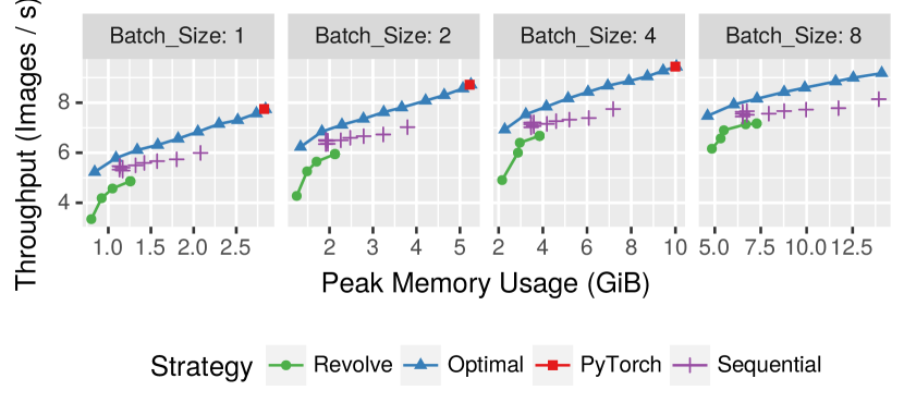
Figure 3: Experimental results for the ResNet network with depth 101 and image size 1000.

5.4 Experimental Results

All plots corresponding to above described experiments are available in the supplementary material. For the sake of conciseness, we only present here a representative selection of the results; the behavior on other experiments is very similar. All plots have the same structure: for a given set of parameters (network, depth, image size and batch size), we plot for each strategy the achieved throughput (in terms of images per second) against the peak memory usage. The square red dot represents the performance obtained by the standard PyTorch strategy, and its absence from the graph means that a memory overflow error was encountered when attempting to execute it. Purple crosses represent the results obtained with the sequential strategy for different number of segments. The blue line with triangles shows the result obtained with our optimal strategy. The green line with circles show the result obtained with the revolve algorithm. We draw lines to emphasize the fact that these strategies can be given any memory limit as input, whereas the result of sequential is inherently tied to a discrete number of segments. We provide a representative selection of results in Figures 3 to 5, and the complete results can be found in Figures 6 to 13 at the end of the paper.

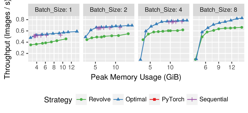
Figure 4: Experimental results for the ResNet network with depth 1001 and image size 224.

Figure 3 shows the results for the ResNet neural network with depth of $101$, with image size $1000\times 1000$ and batch size $1$, $2$, $4$, and $8$. For a batch size of $1$, PyTorch strategy has a memory peak consumption of $2.83$ GiB which is enough to fit on this GPU. However, when the batch size is $8$, PyTorch strategy fails to compute the back-propagation due to memory limitations. The sequential strategy offers a discrete alternative by dividing the chain into a given number of segments (in this case from $2$ to $11$). For every batch size, the best throughput is reached when the number of segments is equal to $2$. For instance, when the batch size is $8$, the throughput of the sequential strategy with $2$ segments is on average $8.13$ images/s with a memory peak consumption of $13.91$ GiB. The optimal strategy offers a continuous alternative by implementing the best checkpointing strategy for any given memory bound. We can see that for a given memory peak, the optimal strategy outperforms the sequential strategy by 15% on average. For instance, when the batch size is $8$, the maximum throughput achieved by the optimal strategy is $9.18$ images/s. The previous revolve algorithm provides a continuous approach as well. However, it requires to compute each forward operation at least twice (once in the forward phase, once before the backward operation), which incurs a much lower throughput than both other solutions. Furthermore, since this algorithm does not consider saving the larger $\bar{a}$ values, it is unable to make use of larger memory sizes.

Figure 4 displays the same results for the ResNet with depth of $1001$ and image size of $224\times 224$. This setup requires much more memory and the PyTorch strategy fails even when the batch size is $1$. The sequential strategy requires at least $6$ segments for batch size $1$, $10$ segments for batch size $2$, and $18$ segments for batch size $4$, and cannot perform the back-propagation when the batch size is $8$. Not only does the optimal strategy outperform the sequential strategy when it does not fail but it offers a stable solution to train the neural network even with a larger batch size, which allows to increase the achieved throughput thanks to a better GPU efficiency (0.82 for PyTorch whereas the highest throughput achieved by sequential is 0.76). It is interesting to note that based on the parameters estimated by our tool, running the setting with batch size 8 with the PyTorch strategy would require 225 GiB of memory, and achieve a throughput of 1.1 images/s. Additional results in Figure 13 also show that optimal allows to run this large network even with medium and large image sizes.

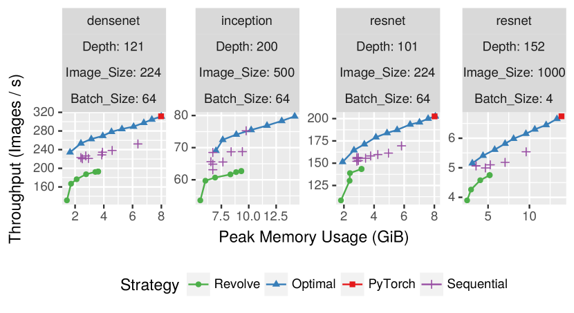
Figure 5: Experimental results for several situations.

All these conclusions hold for every tested neural network and parameters. Figure 5 displays some of them and shows that the behavior of the optimal strategy is stable on various network sizes and image sizes. To summarize, we also compute the ratio between the highest throughput obtained by sequential and the throughput achieved by optimal with the corresponding memory usage. On average over all tested sets of parameters, optimal achieves 17.2% higher throughput.

6 Conclusion

This document describes a new checkpointing strategy that leverages operations available in DNN frameworks with the capabilities of autograd functions. We carefully model back-propagation and we propose a dynamic programming algorithm which computes the optimal persistent schedule for any sequentialized network and its implementation for any sequential Pytorch module. Using in-depth experiments, we compare achieved results against (i) a periodic checkpointing strategy available in PyTorch and (ii) an optimal persistent strategy adapted from the Automatic Differentiation literature to a fully heterogeneous setting, but which does not use all the capabilities available in DNN frameworks. We show that our implementation consistently outperforms these two checkpointing strategies, for a large class of networks, image sizes and batch sizes. Our fully automatic tool increases throughput by an average of 17.2% compared to its best competitor, with better flexibility since it offers the ability to specify an arbitrary memory limit. Our tool therefore allows you to use larger models, larger batches or larger images while automatically adapting to the memory of the training device. In our future work, we want to study the advantages of our approach in combination with other strategies developed to address memory limitations such as model parallelism, activation offloading and domain decomposition.

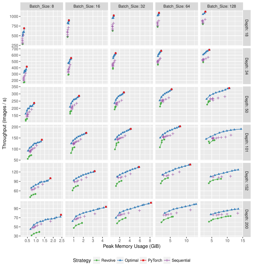
Figure 6: Results for Resnet with image size 224, for different depths and batch sizes.

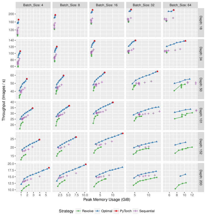
Figure 7: Results for Resnet with image size 500, for different depths and batch sizes.

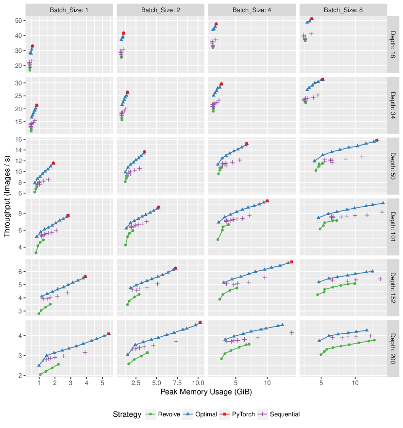
Figure 8: Results for Resnet with image size 1000, for different depths and batch sizes.

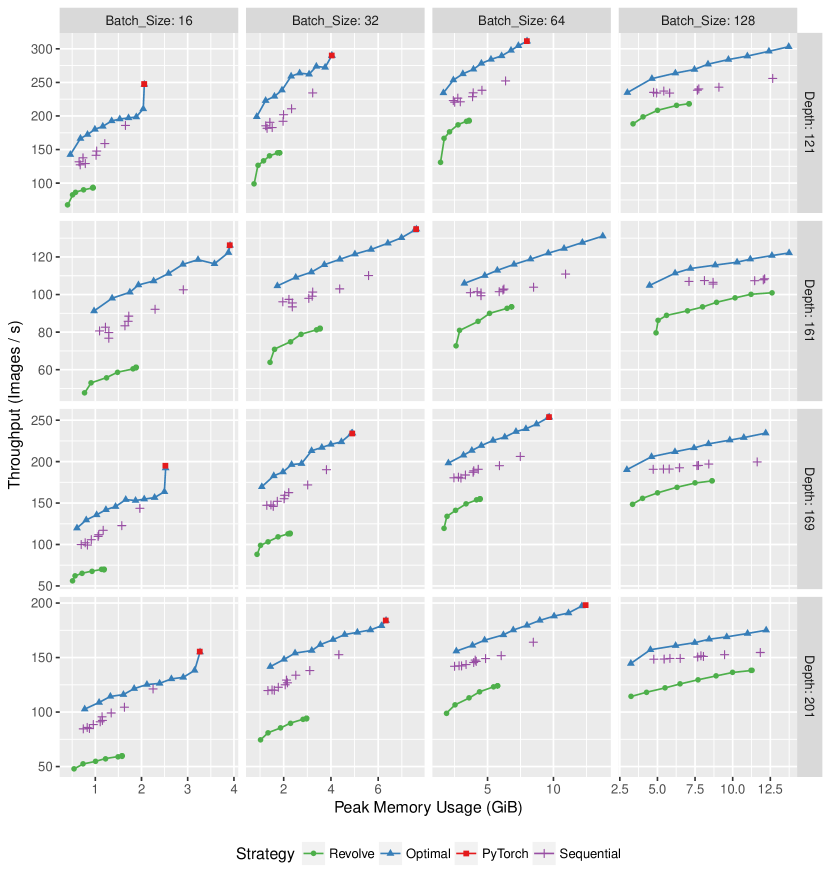
Figure 9: Results for Densenet with image size 224, for different depths and batch sizes.

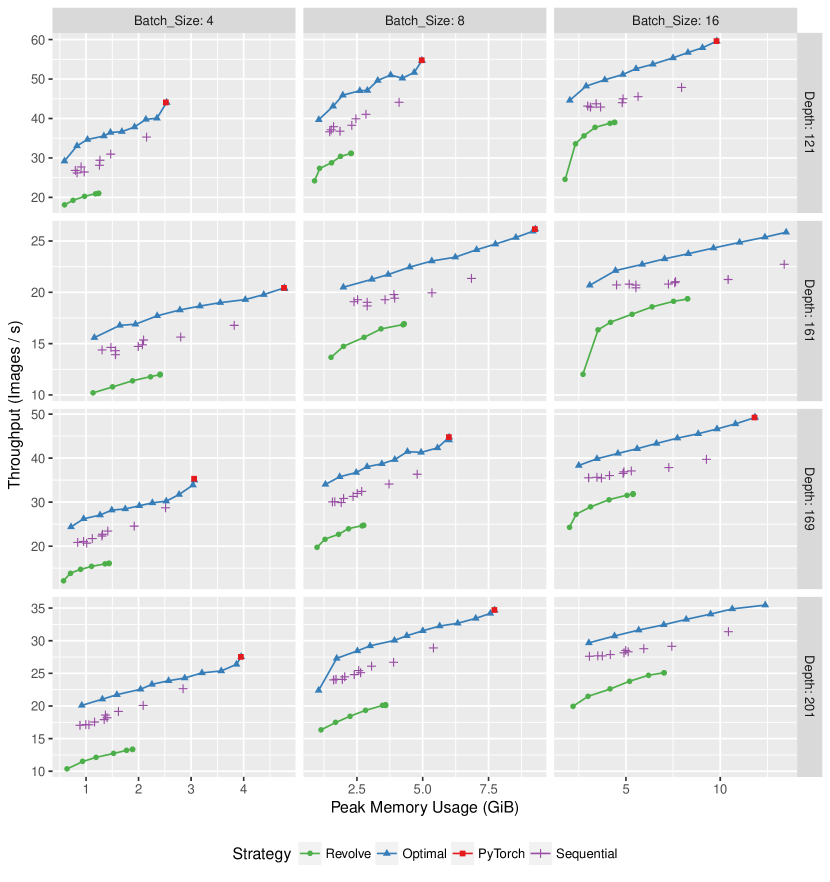
Figure 10: Results for Densenet with image size 500, for different depths and batch sizes.

Figure 11: Results for Densenet with image size 1000, for different depths and batch sizes.

Figure 12: Results for Inception v3 for different image sizes and batch sizes.

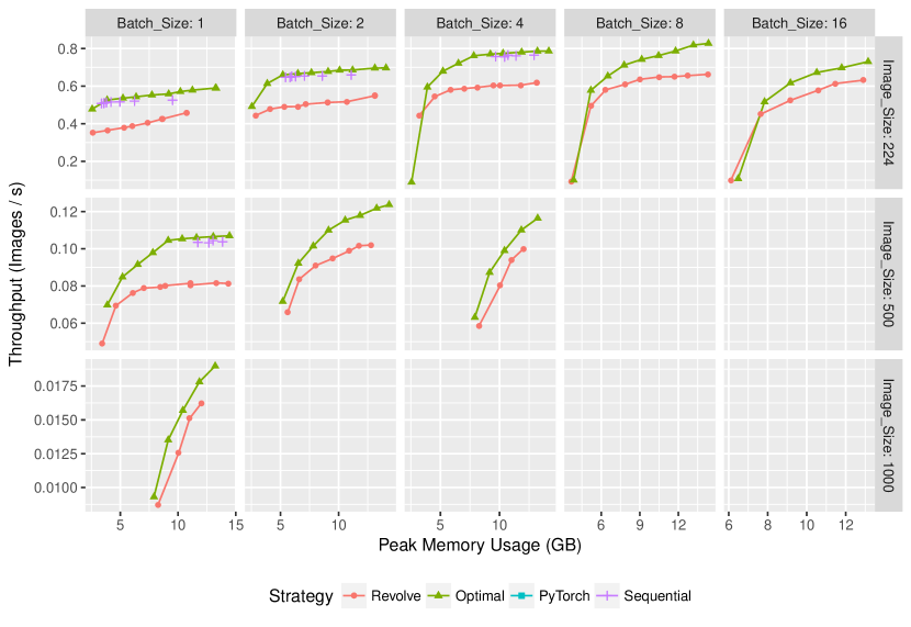
Figure 13: Results for Resnet 1001, for different image sizes and batch sizes.

References

- [1] Periodic checkpointing in pytorch, 2018. https://pytorch.org/docs/stable/checkpoint.html.
- [2] Pytorch memory optimizations via gradient checkpointing, 2018. https://github.com/prigoyal/pytorch_memonger.
- [3] Aupy, G., Herrmann, J., Hovland, P., and Robert, Y. Optimal multistage algorithm for adjoint computation. SIAM Journal on Scientific Computing 38, 3 (2016), 232–255.
- [4] Beaumont, O., Herrmann, J., Pallez, G., and Shilova, A. Optimal Memory-aware Backpropagation of Deep Join Networks. Research Report RR-9273, Inria, May 2019.
- [5] Chang, B., Meng, L., Haber, E., Ruthotto, L., Begert, D., and Holtham, E. Reversible architectures for arbitrarily deep residual neural networks. In Thirty-Second AAAI Conference on Artificial Intelligence (2018).
- [6] Chen, T., Xu, B., Zhang, C., and Guestrin, C. Training deep nets with sublinear memory cost. arXiv preprint arXiv:1604.06174 (2016).
- [7] Das, D., Avancha, S., Mudigere, D., Vaidynathan, K., Sridharan, S., Kalamkar, D., Kaul, B., and Dubey, P. Distributed deep learning using synchronous stochastic gradient descent. arXiv preprint arXiv:1602.06709 (2016).
- [8] Dean, J., Corrado, G., Monga, R., Chen, K., Devin, M., Mao, M., Senior, A., Tucker, P., Yang, K., Le, Q. V., et al. Large scale distributed deep networks. In Advances in neural information processing systems (2012), pp. 1223–1231.
- [9] Dryden, N., Maruyama, N., Benson, T., Moon, T., Snir, M., and Van Essen, B. Improving strong-scaling of cnn training by exploiting finer-grained parallelism. In IEEE International Parallel and Distributed Processing Symposium (2019), IEEE Press.
- [10] Gomez, A. N., Ren, M., Urtasun, R., and Grosse, R. B. The reversible residual network: Backpropagation without storing activations. In Advances in neural information processing systems (2017), pp. 2214–2224.
- [11] Griewank, A. On automatic differentiation. Mathematical Programming: Recent Developments and Applications 6, 6 (1989), 83–107.
- [12] Griewank, A., and Walther, A. Algorithm 799: Revolve: an implementation of checkpointing for the reverse or adjoint mode of computational differentiation. ACM Transactions on Mathematical Software (TOMS) 26, 1 (2000), 19–45.
- [13] Griewank, A., and Walther, A. Evaluating derivatives: principles and techniques of algorithmic differentiation, vol. 105. Siam, 2008.
- [14] Gruslys, A., Munos, R., Danihelka, I., Lanctot, M., and Graves, A. Memory-efficient backpropagation through time. In Advances in Neural Information Processing Systems (2016), pp. 4125–4133.
- [15] He, K., Zhang, X., Ren, S., and Sun, J. Identity mappings in deep residual networks. In Computer Vision – ECCV 2016 (2016), Springer International Publishing, pp. 630–645.
- [16] Howard, A. G., Zhu, M., Chen, B., Kalenichenko, D., Wang, W., Weyand, T., Andreetto, M., and Adam, H. Mobilenets: Efficient convolutional neural networks for mobile vision applications. arXiv preprint arXiv:1704.04861 (2017).
- [17] Hubara, I., Courbariaux, M., Soudry, D., El-Yaniv, R., and Bengio, Y. Quantized neural networks: Training neural networks with low precision weights and activations. The Journal of Machine Learning Research 18, 1 (2017), 6869–6898.
- [18] Pleiss, G., Chen, D., Huang, G., Li, T., van der Maaten, L., and Weinberger, K. Q. Memory-efficient implementation of densenets. arXiv preprint arXiv:1707.06990 (2017).
- [19] Rastegari, M., Ordonez, V., Redmon, J., and Farhadi, A. Xnor-net: Imagenet classification using binary convolutional neural networks. In European Conference on Computer Vision (2016), Springer, pp. 525–542.
- [20] Rhu, M., Gimelshein, N., Clemons, J., Zulfiqar, A., and Keckler, S. W. vdnn: Virtualized deep neural networks for scalable, memory-efficient neural network design. In The 49th Annual IEEE/ACM International Symposium on Microarchitecture (2016), IEEE Press, p. 18.
- [21] Rota Bulò, S., Porzi, L., and Kontschieder, P. In-place activated batchnorm for memory-optimized training of dnns. In Proceedings of the IEEE Conference on Computer Vision and Pattern Recognition (2018), pp. 5639–5647.
- [22] S B, S., Garg, A., and Kulkarni, P. Dynamic memory management for gpu-based training of deep neural networks. In 2019 IEEE International Parallel and Distributed Processing Symposium (IPDPS) (2016), IEEE Press.
- [23] Siskind, J. M., and Pearlmutter, B. A. Divide-and-conquer checkpointing for arbitrary programs with no user annotation. Optimization Methods and Software 33, 4-6 (2018), 1288–1330.
- [24] Verhelst, M., and Moons, B. Embedded deep neural network processing: Algorithmic and processor techniques bring deep learning to iot and edge devices. IEEE Solid-State Circuits Magazine 9, 4 (2017), 55–65.
- [25] Walther, A., and Griewank, A. Advantages of binomial checkpointing for memory-reduced adjoint calculations. In Numerical mathematics and advanced applications. Springer, 2004, pp. 834–843.
- [26] Zhang, X., Zhou, X., Lin, M., and Sun, J. Shufflenet: An extremely efficient convolutional neural network for mobile devices. In Proceedings of the IEEE Conference on Computer Vision and Pattern Recognition (2018), pp. 6848–6856.