Solving Inverse Wave Scattering with Deep Learning

Abstract

This paper proposes a neural network approach for solving two classical problems in the two-dimensional inverse wave scattering: far field pattern problem and seismic imaging. The mathematical problem of inverse wave scattering is to recover the scatterer field of a medium based on the boundary measurement of the scattered wave from the medium, which is high-dimensional and nonlinear. For the far field pattern problem under the circular experimental setup, a perturbative analysis shows that the forward map can be approximated by a vectorized convolution operator in the angular direction. Motivated by this and filtered back-projection, we propose an effective neural network architecture for the inverse map using the recently introduced BCR-Net along with the standard convolution layers. Analogously for the seismic imaging problem, we propose a similar neural network architecture under the rectangular domain setup with a depth-dependent background velocity. Numerical results demonstrate the efficiency of the proposed neural networks.

Keywords: Inverse scattering; Helmholtz equation; Far field pattern; Seismic imaging; Neural networks; Convolutional neural network.

1 Introduction

Inverse wave scattering is the problem of determining the intrinsic property of an object based on the data collected from the object scatters incoming waves under the illumination of an incident wave, which can be acoustic, electromagnetic, or elastic. In most cases, inverse wave scattering is non-intrusive to the object under study and therefore it has a wide range of applications including radar imaging [8], sonar imaging [32], seismic exploration [65], geophysics exploration [64], and medicine imaging [35] and so on.

Background.

We focus on the time harmonic acoustic inverse scattering in two dimensions. Let $\Omega$ be a compact domain of interest. The inhomogeneous media scattering problem at a fixed frequency $\omega$ is modeled by the Helmholtz equation

$$Lu:=\bigg{(}-\Delta-\frac{\omega^{2}}{c^{2}(x)}\bigg{)}u,$$ (1.1)

where $c(x)$ is the unknown velocity field. Assume that there exists a known background velocity $c_{0}(x)$ such that $c(x)$ is identical to $c_{0}(x)$ outside the domain $\Omega$. By introducing the scatterer $\eta(x)$:

$$\eta(x)=\frac{\omega^{2}}{c(x)^{2}}-\frac{\omega^{2}}{c_{0}(x)^{2}}$$ (1.2)

compactly supported in $\Omega$, one can equivalently work with $\eta(x)$ instead of $c(x)$. Note that in this definition $\eta(x)$ scales quadratically with the frequency $\omega$. However, as $\omega$ is assumed to be fixed throughout this paper, this scaling does not affect our discussion.

In order to recover the unknown $\eta(\cdot)$, a typical setup of an experiment is as follows. For each source $s$ from a source set $S$, one specifies an incoming wave (typically either a plane wave or a point source) and propagates the wave to the scatterer $\eta(\cdot)$. The scattered wave field $u^{s}(x)$ is then recorded at each receiver $r$ from a receiver set $R$ (typically placed at the domain boundary or infinity). The whole dataset, indexed by both the source $s$ and the receiver $r$, is denoted by $\{d(s,r)\}_{s\in S,r\in R}$. The forward problem is to compute $d(s,r)$ given $\eta(x)$. The inverse scattering problem is to recover $\eta(x)$ given $d(s,r)$,

Both the forward and inverse problems are computationally quite challenging, and in the past several decades a lot of research has been devoted to their numerical solution [21, 22]. For the forward problem, the time-harmonic Helmholtz equation, especially in the high-frequency regime $\omega\gg 1$, is hard to solve mainly due to two reasons: (1) the Helmholtz operator has a large number of both positive and negative eigenvalues, with some close to zero; (2) a large number of degrees of freedom are required for discretization due to the Nyquist sampling rate. In recent years, quite a few methods have been developed for rapid solutions of Helmholtz operator [29, 18, 20, 19, 51]. The inverse problem is more difficult for numerical solution, due to the nonlinearity of the problem. For the methods based on optimization, as the loss landscape is highly non-convex (for example, the cycle skipping problem in seismic imaging [55]), the optimization can get stuck at a local minimum with rather large loss value. Other popular methods include the factorization method and the linear sampling method [44, 11, 9].

A deep learning approach.

Deep learning (DL) has recently become the state-of-the-art approach in many areas of machine learning and artificial intelligence, including computer vision, image processing, and speech recognition [36, 46, 31, 54, 49, 62, 48, 61]. From a technical point of view, this success can be attributed to several key developments: neural networks (NNs) as a flexible framework for representing high-dimensional functions and maps, efficient general software packages such as Tensorflow and Pytorch, computing power provided by GPUs and TPUs, and effective algorithms such as back-propagation (BP) and stochastic gradient descent (SGD) for tuning the model parameters,

More recently, deep neural networks (DNNs) have been increasingly applied to scientific computing and computational engineering, particularly for PDE-related problems [41, 6, 33, 25, 3, 58, 47, 28]. One direction focuses on the low-dimensional parameterized PDE problems by representing the nonlinear map from the high-dimensional parameters of the PDE solution using DNNs [52, 34, 41, 25, 24, 23, 50, 4]. A second direction takes DNN as an ansatz for high-dimensional PDEs [60, 10, 33, 42, 17] since DNNs offer a powerful tool for approximating high-dimensional functions and densities [15].

As an important example of the first direction, DNNs have been widely applied to inverse problems [43, 37, 40, 2, 53, 63, 26, 27, 59]. For the forward problem, as applying neural networks to input data can be carried out rapidly due to novel software and hardware architectures, the forward solution can be significantly accelerated once the forward map is represented with a DNN. For the inverse problem, two critical computational issues are the choices of the solution algorithm and the regularization term. DNNs can help on both aspects: first, concerning the solution algorithm, due to its flexibility in representing high-dimensional functions, DNN can potentially be used to approximate the full inverse map, thus avoiding the iterative solution process; second, concerning the regularization term, DNNs often can automatically extract features from the data and offer a data-driven regularization prior.

This paper applies the deep learning approach to inverse wave scattering by representing the whole inverse map using neural networks. Two cases are considered here: (1) far field pattern and (2) seismic imaging. In our relatively simple setups, the main difference between the two is the source and receiver configurations: in the far field pattern, the sources are plane waves and the receivers are regarded as placed at infinity; in the seismic imaging, both the sources and receivers are placed at the top surface of the survey domain.

In each case, we start with a perturbative analysis of the forward map, which shows that the forward map contains a vectorized one-dimensional convolution, after appropriate reparameterization of the unknown coefficient $\eta(x)$ and the data $d(s,r)$. This observation suggests to represent the forward map from $\eta$ to $d$ by a one-dimensional convolution neural network (with multiple channels). The filtered back-projection method [56] approximates the inverse map with the adjoint of the forward map followed by a pseudo-differential filtering. This suggests an inverse map architecture of reversing the forward map network followed by a simple two-dimensional convolution neural network. For both cases, the resulting neural networks enjoy a relatively small number of parameters, thanks to the convolutional structure. This small number of parameters also allows for accurate and rapid training, even with a somewhat limited dataset.

Organization.

This rest of the paper is organized as follows. Section 2 discusses the far field pattern problem. Section 3 considers the seismic imaging problem. Section 4 concludes with some discussions for future work.

2 Far field pattern

2.1 Mathematics analysis

In the far field pattern case, the background velocity field $c_{0}(x)$ is constant, and without loss of generality, equal to one. We introduce the base operator $L_{0}=-\Delta-\omega^{2}/c_{0}^{2}=-\Delta-\omega^{2}$ and write $L$ in a perturbative way as

$$L=L_{0}-\eta.$$ (2.1)

The sources are parameterized by $s\in S=[0,2\pi)$. For each source $s$, the incoming wave is a plane wave $e^{i\omega\widehat{s}\cdot x}$ with the unit direction given by $\widehat{s}=(\cos(s),\sin(s))\in\mathbb{S}^{1}$. The scattered wave $u^{s}(x)$ satisfies the following equation

$$(L_{0}-\eta)(e^{i\omega\widehat{s}\cdot x}+u^{s}(x))=0,$$ (2.2)

along with the Sommerfeld radiation boundary condition at infinity [14]. The receivers are also indexed by $r\in R=[0,2\pi)$. The far field pattern at the unit direction $\widehat{r}=(\cos(r),\sin(r))\in\mathbb{S}^{1}$ is defined as

$$\widehat{u}^{s}(r)\equiv\lim_{\rho\rightarrow\infty}\sqrt{\rho}e^{-i\omega\rho}u^{s}(\rho\cdot\widehat{r}).$$

The recorded data is the set of far field pattern from all incoming directions: $d(s,r)\equiv\widehat{u}^{s}(r)$ for $r\in R$ and $s\in S$.

In order to understand better the relationship between $\eta(x)$ and $d(s,r)$, we perform a perturbative analysis for small $\eta$. Expanding (2.2) leads to

$$(L_{0}u^{s})(x)=\eta(x)e^{i\omega\widehat{s}\cdot x}+\ldots,$$

where $\ldots$ stands for higher order terms in $\eta$. Letting $G_{0}=L_{0}^{-1}$ be the Green’s functions of the free-space Helmholtz operator $L_{0}$, we get

$$u^{s}(y)=\int G_{0}(y-x)\eta(x)e^{i\omega\widehat{s}\cdot x}\,\mathrm{d}x+\ldots$$

Using the expansion at infinity

$$G_{0}(z)=\frac{e^{i\omega|z|}+o(1)}{\sqrt{|z|}},$$

we arrive at

$$\widehat{u}^{s}(r)=\lim_{\rho\rightarrow\infty}\sqrt{\rho}e^{-i\omega\rho}u^{s}(\rho\cdot\widehat{r})\approx\lim_{\rho\rightarrow\infty}\int\frac{e^{i\omega(\rho-\widehat{r}\cdot x)}}{\sqrt{\rho}}\sqrt{\rho}e^{-i\omega\rho}\eta(x)e^{i\omega\widehat{s}\cdot x}\,\mathrm{d}x\\ =\int e^{-i\omega(\widehat{r}-\widehat{s})\cdot x}\eta(x)\,\mathrm{d}x\equiv d_{1}(s,r),$$ (2.3)

where the notation $d_{1}(s,r)$ stands for the first order approximation to $d(s,r)$ in $\eta$.

2.1.1 Problem setup

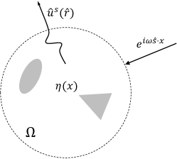
Figure 1: Illustration of the incoming and outgoing waves for a far field pattern problem. The scatterer $\eta(x)$ is compactly supported in the domain $\Omega$. The incoming plane wave points at direction $\widehat{s}=(\cos(s),\sin(s))$. The far field pattern is sampled at each receiver direction $\widehat{r}=(\cos(r),\sin(r))$.

For the far field pattern problem, we are free to treat the domain $\Omega$ as the unit disk centered at origin (by appropriate rescaling and translation), as illustrated in Fig. 1. In a commonly used setting, the sources and receivers are uniformly sampled in $\mathbb{S}^{1}$: $s=\frac{2\pi j}{N_{s}}$, $j=0,\dots,N_{s}-1$ and $r=\frac{2\pi k}{N_{r}}$, $k=0,\dots,N_{r}-1$, where $N_{s}=N_{r}$ for simplicity.

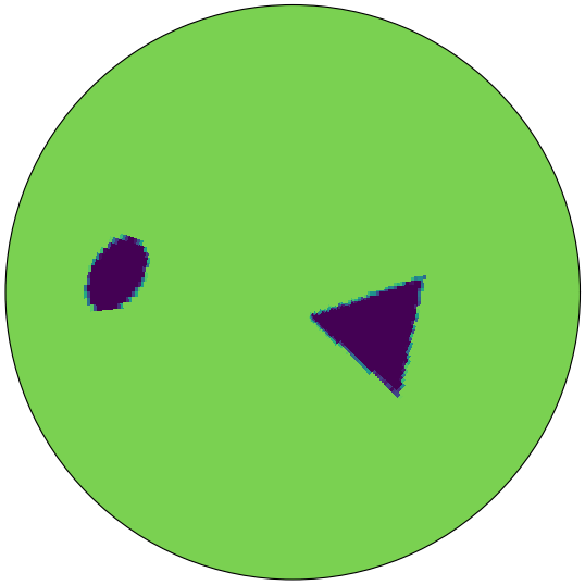
(a) $\eta(x)$

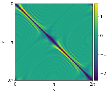
(b) $\Re(d(s,r))$

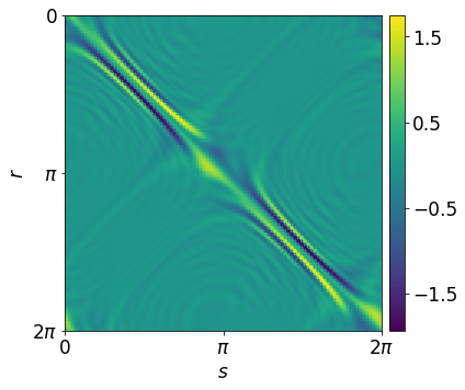
(c) $\Im(d(s,r))$

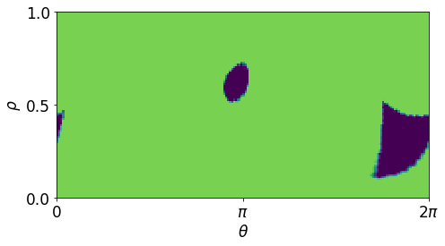
(d) $\eta(\theta,\rho)$

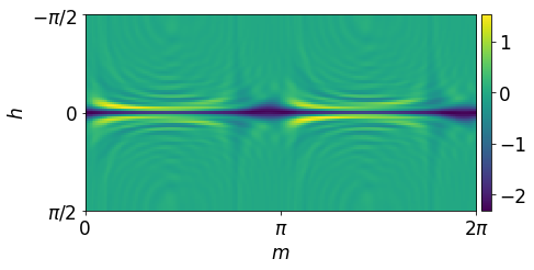
(e) $\Re(d(m,h))$

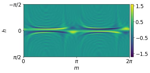
(f) $\Im(d(m,h))$

Figure 2: Visualization of the scatterer field $\eta$ and the measurement data $d$. The upper figures are the scatterer and the real and imaginary parts of the measurement data $d$, respectively. The lower-left figure is the scatterer in the polar coordinates. The next two lower figures are the real and imaginary parts of the measurement data after the change of variable, respectively.

2.1.2 Forward map

Since the domain $\Omega$ is the unit disk, it is convenient to work with the problem in the polar coordinates. Let $x=(\rho\cos(\theta),\rho\sin(\theta))$, where $\rho\in[0,1]$ is the radial coordinate and $\theta\in[0,2\pi)$ is the angular one. Due to the circular tomography geometry that $r,s\in[0,2\pi)$, it is convenient to reparameterize the measurement data by a change of variables

$$m=\frac{r+s}{2},h=\frac{r-s}{2},\quad\text{or equivalently}\quad r=m+h,s=m-h,$$ (2.4)

where all the variables $m,h,r,s$ are understood modulus $2\pi$. Figure 2 presents an example of the scatterer field $\eta(x)$ and the measurement data $d(s,r)$ in the original and transformed coordinates.

With a bit abuse of notation, we can redefine the measurement data

$$d(m,h)\equiv d(s,r)|_{s=m-h,r=m+h},$$ (2.5)

and so does $d_{1}(m,h)$. At the same time, we redefine

$$\eta(\theta,\rho)=\eta(\rho\cos(\theta),\rho\sin(\theta)$$

in the polar coordinates. Since the first order approximation $d_{1}(m,h)$ is linearly dependent on $\eta(\theta,\rho)$, there exists a kernel distribution $K(m,h,\theta,\rho)$ such that

$$d_{1}(m,h)=\int_{0}^{1}\int_{0}^{2\pi}K(m,h,\theta,\rho)\eta(\theta,\rho)\,\mathrm{d}\rho\,\mathrm{d}\theta.$$ (2.6)

Since the domain is the unit disk centered at origin and the background velocity field $c_{0}=1$ is constant, the whole problem is equivariant to rotation. In this case, the system can be dramatically simplified due to the following proposition.

Proposition 1.

There exists a function $\kappa(h,\rho,\cdot)$ periodic in the last parameter such that $K(m,h,\theta,\rho)=\kappa(h,\rho,m-\theta)$ or equivalently,

$$d_{1}(m,h)=\int_{0}^{1}\int_{0}^{2\pi}\kappa(h,\rho,m-\theta)\eta(\rho,\theta)\,\mathrm{d}\theta\,\mathrm{d}\rho.$$ (2.7)

Proof.

A simple calculation shows that the phase $(\widehat{r}-\widehat{s})\cdot x$ now becomes

$$(\widehat{r}-\widehat{s})\cdot x=(\widehat{(m+h)}-\widehat{(m-h)})\cdot(\rho\cos(\theta),\rho\sin(\theta))=2\rho\sin(h)\sin(\theta-m).$$

Therefore, 2.3 turns to

$$d_{1}(m,h)=\int_{0}^{1}\int_{0}^{2\pi}\left(\rho e^{2i\rho\omega\sin h\sin(m-\theta)}\right)\eta(\theta,\rho)\,\mathrm{d}\theta\,\mathrm{d}\rho.$$

Setting $\kappa(h,\rho,y)=\rho e^{2i\rho\omega\sin h\sin(y)}$ completes the proof. ∎

Proposition 1 shows that $K$ acts on $\eta$ in the angular direction by a convolution, which allows us to evaluate the map $\eta(\theta,\rho)\to d_{1}(m,h)$ by a family of 1D convolutions, parameterized $\rho$ and $h$.

Discretization.

Until now, the discussion is in the continuous space. The discretization and solution method of the Helmholtz equation will be discussion along with the numerical results. With a slight abuse of notation, the same symbols will be used to denote the discrete version of the continuous data and kernels and the discrete version of Equations 2.3 and 2.7 takes the form

$$d(m,h)\approx\sum_{\rho,\theta}K(m,h,\theta,\rho)\eta(\theta,\rho)=\sum_{\rho}\left(\kappa(h,\rho,\cdot)*\eta(\cdot,\rho)\right)(m).$$ (2.8)

2.2 Neural network

Forward map.

The perturbative analysis shows that, when $\eta$ is sufficiently small, the forward map $\eta(\theta,\rho)\to d(m,h)$ can be approximated with 2.8. In terms of the NN architecture, for small $\eta$, by taking $h$ and $\rho$ directions as the channel dimension, the forward map 2.8 can be approximated by a one-dimensional (non-local) convolution layer. For larger $\eta$, this linear approximation is no longer accurate, which can be addressed by increasing the number of convolution layers and including nonlinear activations for the neural network of 2.8.

1:$c$, $N_{\mathrm{cnn}}\in\mathbb{N}^{+}$, $\eta\in\mathbb{R}^{N_{\theta}\times N_{\rho}}$

2:$d\in\mathbb{R}^{N_{s}\times N_{h}}$

3:$\xi={{\sf{Conv1d}}}[c,1,{{\sf{id}}}](\eta)$ with $\rho$ as the channel direction $\triangleright$ Resampling $\eta$ to fit for BCR-Net

4:$\zeta={\text{{\sf{BCR-Net}}}}[c,N_{\mathrm{cnn}}](\xi)$ $\triangleright$ Use BCR-Net to implement the convolutional neural network.

5:$d={{\sf{Conv1d}}}[N_{h},1,{{\sf{id}}}](\zeta)$ $\triangleright$ Reconstruct the result $d$ from the output of BCR-Net.

6:return $d$

Algorithm 1 Neural network architecture for the forward map $\eta\to d$.

The number of channels, denoted by $c$, is quite problem-dependent and will be discussed in the numerical section. Notice that the convolution between $\eta$ and $d$ is global in the angular direction. In order to represent global interactions, the window size $w$ of the convolution layer and the number of layers $N_{\mathrm{cnn}}$ must satisfy the constraint

$$wN_{\mathrm{cnn}}\geq N_{\theta},$$ (2.9)

where $N_{\theta}$ is number of discretization points on the angular direction. A simple calculation shows that the number of parameters of the neural network is $O(wN_{\mathrm{cnn}}c^{2})\sim O(N_{\theta}c^{2})$. The recently introduced BCR-Net [23] has been demonstrated to require fewer number of parameters and provide good efficiency for such interactions. Therefore, we replace the convolution layers with the BCR-Net in our architecture. The resulting neural network architecture for the forward map is summarized in Algorithm 1 with an estimate of $O(c^{2}\log(N_{\theta})N_{\mathrm{cnn}})$ parameters. The components of Algorithm 1 are detailed below.

• $\xi={{\sf{Conv1d}}}[c,w,\phi](\eta)$, which maps $\eta\in\mathbb{R}^{N_{\theta}\times N_{\rho}}$ to $\xi\in\mathbb{R}^{N_{\theta}\times c}$ is the one-dimensional convolution layer with window size $w$, channel number $c$, activation function $\phi$ and period padding on the first direction.

• BCR-Net is a multiscale neural network motivated by the data-sparse nonstandard wavelet representation of the linear operators [7]. It processes the information at different scale separately and each scale can be understood as a local convolutional neural network. The one-dimensional $\zeta={\text{{\sf{BCR-Net}}}}[c,N_{\mathrm{cnn}}](\xi)$ maps $\xi\in\mathbb{R}^{N_{\theta}\times c}$ to $\zeta\in\mathbb{R}^{N_{\theta}\times c}$ where $c$ is the number of wavelets in each scale and $N_{\mathrm{cnn}}$ denotes the number of layers in the local convolutional neural network in each scale. The readers are referred to [23] for more details on the BCR-Net.

Inverse map.

As we have seen, if $\eta$ is sufficiently small, the forward map can be approximated by $d\approx K\eta$, the operator notation of the discretization 2.8. Here $\eta$ is a vector indexed by $(\theta,\rho)$, $d$ is a vector indexed by $(m,h)$, and $K$ is a matrix with row indexed by $(m,h)$ and column indexed by $(\theta,\rho)$.

The filtered back-projection method [56] suggests the following formula to recover $\eta$:

$$\eta\approx(K^{\mathsf{T}}K+\epsilon I)^{-1}K^{\mathsf{T}}d,$$ (2.10)

where $\epsilon$ is a regularization parameter. The first piece $K^{\mathsf{T}}d$ can also be written as a family of convolutions as well

$$(K^{\mathsf{T}}d)(\theta,\rho)=\sum_{h}(\kappa(h,\rho,\cdot)*d(\cdot,h))(\theta).$$ (2.11)

The application of $K^{\mathsf{T}}$ to $d$ can be approximated with a neural network similar to the one for $K$ in Algorithm 1, by reversing the order. The second piece $(K^{\mathsf{T}}K+\epsilon I)^{-1}$ is a pseudo-differential operator in the $(\theta,\rho)$ space and it is implemented with several two-dimensional convolutional layers for simplicity. Putting two pieces together, the resulting architecture for the inverse map is summarized in Algorithm 2 and illustrated in Fig. 3. Here, ${{\sf{Conv2d}}}[c_{2},w,\phi]$ used in Algorithm 2 is a two-dimensional convolution layer with window size $w$, channel number $c_{2}$, activation function $\phi$ and periodic padding on the first direction and zero padding on the second direction. The selection of the hyper-parameters in Algorithm 2 will be discussed in the numerical section.

1:$c,c_{2}$, $w$, $N_{\mathrm{cnn}}$, $N_{\mathrm{cnn}2}\in\mathbb{N}^{+}$, $d\in\mathbb{R}^{N_{s}\times N_{h}}$

2:$\eta\in\mathbb{R}^{N_{\theta}\times N_{\rho}}$

3:# Application of $K^{\mathsf{T}}$ to $d$

4:$\zeta={{\sf{Conv1d}}}[c,1,{{\sf{id}}}](d)$ with $h$ as the channel direction

5:$\xi={\text{{\sf{BCR-Net}}}}[c,N_{\mathrm{cnn}}](\zeta)$

6:$\xi^{(0)}={{\sf{Conv1d}}}[N_{\rho},1,{{\sf{id}}}](\xi)$

7:# Application of $(K^{\mathsf{T}}K+\epsilon I)^{-1}$

8:for $k$ from $1$ to $N_{\mathrm{cnn}2}-1$ do

9:    $\xi^{(k)}={{\sf{Conv2d}}}[c_{2},w,{{\sf{ReLU}}}](\xi^{(k-1)})$

10:end for

11:$\eta={{\sf{Conv2d}}}[1,w,{{\sf{id}}}](\xi^{(N_{\mathrm{cnn}2}-1)})$

12:return $d$

Algorithm 2 Neural network architecture for the inverse problem $d\to\eta$.

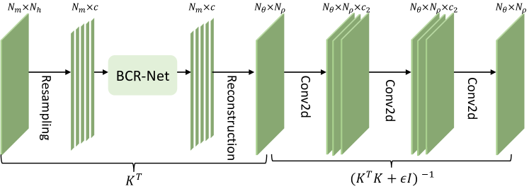
Figure 3: Neural network architecture for the inverse map of far field pattern problem.

2.3 Numerical examples

This section reports the numerical setup and results of the proposed neural network architecture in Algorithm 2 for the inverse map $d\to\eta$.

2.3.1 Experimental setup

Since the scatterer $\eta$ is compactly supported in the unit disk $\Omega$, we embed $\Omega$ into the square domain $[-1,1]^{2}$ and solve the Helmholtz equation (1.1) in the square. In the numerical solution of the Helmholtz equation, we discretize $[-1,1]^{2}$ with a uniform Cartesian mesh with $192$ points in each direction by a finite difference scheme (frequency $\omega=16$ and $12$ points used per wavelength). The perfectly matched layer [5] is used to deal with the Sommerfeld boundary condition and the solution of the discrete system can be accelerated with appropriate preconditioners (for example, [20]).

In the polar coordinates of $\Omega$, $(\theta,\rho)\in[0,2\pi)\times[0,1]$ is partitioned by uniformly Cartesian mesh with $192\times 96$ points, i.e., $N_{\theta}=192$ and $N_{\rho}=96$. Given the values of $\eta$ in the Cartesian grid, the values $\eta(\theta,\rho)$ used in Algorithm 2 in the polar coordinates are computed via linear interpolation.

The number of sources and receivers are $N_{s}=N_{r}=192$. The measurement data $d(s,r)$ is generated by solving the Helmholtz equation $N_{s}$ times with different incident plane wave. For the change of variable of $(s,r)\to(m,h)$, linear interpolation is used to generate the data $d(m,h)$ from $d(s,r)$. In the $(m,h)$ space, $N_{m}=192$ for $m\in[0,2\pi)$ and $N_{h}=96$ for $h\in(-\pi/2,\pi/2)$. Since the measurement data is complex, the real and imaginary parts can be treated separately as two channels. The actual simulation suggests that using only the real part (or the imaginary part) as input for Algorithm 2 is enough to generate good results.

The NN in Algorithm 2 is implemented in Keras [12] on top of TensorFlow [1]. The loss function is taken to be the mean squared error and the optimizer used is Nadam [16]. The parameters of the network are initialized by Xavier initialization [30]. Initially, the batch size and the learning rate is firstly set as $32$ and $10^{-3}$, respectively, and the NN is trained with $100$ epochs. We then increase the batch size by a factor of $2$ till $512$ with the learning rate unchanged, and next decrease the learning rate by a factor $10^{1/2}$ down to $10^{-5}$ with the batch size fixed at $512$. For each batch size and learning rate configuration, the NN is trained with $50$ epochs. The hyper-parameters used for Algorithm 2 are $N_{\mathrm{cnn}}=6$, $N_{\mathrm{cnn}2}=5$, and $w=3\times 3$. The selection of the channel number $c$ will be studied next.

2.3.2 Results

For a fixed $\eta$, $d(m,h)$ stands for the exact measurement data solved by numerical discretization of 1.1. The prediction of the NN from $d(m,h)$ is denoted by $\eta^{\mathrm{NN}}$. The metric for the prediction is the peak signal-to-noise ratio (PSNR), which is defined as

$$\mathrm{PSNR}=10\log_{10}\left(\frac{\mathrm{Max}^{2}}{\mathrm{MSE}}\right),~{}~{}\mathrm{Max}=\max_{ij}(\eta_{ij})-\min_{ij}(\eta_{ij}),~{}~{}\mathrm{MSE}=\frac{1}{N_{\theta}N_{\rho}}\sum_{i,j}|\eta_{i,j}-\eta_{i,j}^{\mathrm{NN}}|^{2}.$$ (2.12)

For each experiment, the test PSNR is then obtained by averaging 2.12 over a given set of test samples. The numerical results presented below are obtained by repeating the training process five times, using different random seeds for the NN initialization.

The numerical experiments focus on the shape reconstruction setting [44, 45, 13], where $\eta$ are often piecewise constant inclusions. Here, the scatterer field $\eta$ is assumed to be the sum of ${N_{\mathrm{shape}}}$ piecewise constant shapes. For each shape, it can be either triangle, square or ellipse, its direction is uniformly random over the unit circle, its position is uniformly sampled in the disk, and its inradius is sampled from the uniform distribution $\mathcal{U}(0.1,0.2)$. When a shape is an ellipse, the width and height are sampled from the uniform distribution $\mathcal{U}(0.1,0.2)$ and $\mathcal{U}(0.05,0.1)$. It is also required that each shape lies in the disk and there is no intersection between every two shapes. We generate two dataset for ${N_{\mathrm{shape}}}=2$ and ${N_{\mathrm{shape}}}=4$, and each has $20,480$ samples $\{(\eta_{i},d_{i})\}$ with $16,384$ used for training and the remaining $4,096$ for testing.

Figure 4: The test PSNR for different channel numbers $c$ for the dataset ${N_{\mathrm{shape}}}=4$.

	reference	$\eta^{\mathrm{NN}}$ with $\delta=0$	$\eta^{\mathrm{NN}}$ with $\delta=10\%$	$\eta^{\mathrm{NN}}$ with $\delta=100\%$
ab ${N_{\mathrm{shape}}}$ ${N_{\mathrm{shape}}}=4$ a
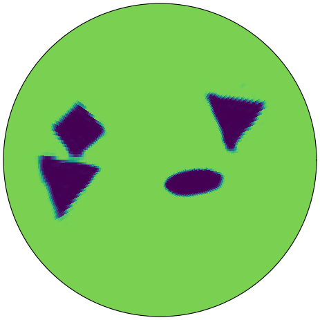
ab ${N_{\mathrm{shape}}}$ ${N_{\mathrm{shape}}}=2$ a

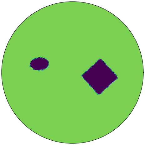
Figure 5: The far field pattern problem. NN prediction of a sample with test data ${N_{\mathrm{shape}}}=4$ (first row) and a sample with ${N_{\mathrm{shape}}}=2$ (second row), at different noise level $\delta=0$, $10\%$ and $100\%$.

	reference	$\eta^{\mathrm{NN}}$ with $\delta=0$	$\eta^{\mathrm{NN}}$ with $\delta=10\%$	$\eta^{\mathrm{NN}}$ with $\delta=100\%$
ab Train: ${N_{\mathrm{shape}}}=2$ Test: n${N_{\mathrm{shape}}}=4$ a
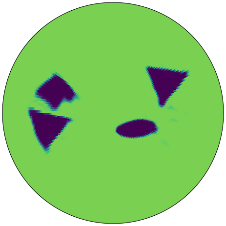
ab Train: ${N_{\mathrm{shape}}}=4$ Test: n${N_{\mathrm{shape}}}=2$ a

Figure 6: The far field pattern problem: NN generalization test. In the first row, the NN is trained by the data with the number of shapes ${N_{\mathrm{shape}}}=2$ with noise level $\delta=0$, $10\%$ or $100\%$ and tested by the data with ${N_{\mathrm{shape}}}=4$ at the same noise level. In the second row, the NN is trained by the data with ${N_{\mathrm{shape}}}=4$ and tested by the data with ${N_{\mathrm{shape}}}=2$.

We first study the choice of channel number $c$ in Algorithm 2. Figure 4 presents the test PSNR and the number of parameters for different channel number $c$ for the dataset ${N_{\mathrm{shape}}}=4$. As the channel number $c$ increases, the test PSNR first increases consistently and then saturates. Note that the number of parameters of the neural network is $O(c^{2}\log(N_{\theta})N_{\mathrm{cnn}})$. The choice of $c=24$ offers a reasonable balance between accuracy and efficiency, and the total number of parameters is $439$K.

To model the uncertainty in the measurement data, we introduce noises to the measurement data by defining $d_{i}^{\delta}\equiv(1+Z_{i}\delta)d_{i}$, where $Z_{i}$ is a Gaussian random variable with zero mean and unit variance and $\delta$ controls the signal-to-noise ratio. For each noisy level $\delta=0$, $10\%$, $100\%$, an independent NN is trained and tested with the noisy dataset $\{(d_{i}^{\delta},\eta_{i})\}$.

Figure 5 collects, for different noise level $\delta=0$, $10\%$, $100\%$, samples for different ${N_{\mathrm{shape}}}=2$, $4$. The NN is trained with the datasets generated in the same way as the test data. When there is no noise in the measurement data, the NN consistently gives accurate predictions of the scatterer field $\eta$, in the position, shape, and direction of the shapes. In particular, for the case ${N_{\mathrm{shape}}}=4$, the square in the left part of the domain is close to a triangle. The NN is able to distinguish the shapes and gives a clear boundary of each. For the small noise levels, for example, $\delta=10\%$, the boundary of the shapes slightly blurs while the position, direction and shape are still correct. As the noise level $\delta$ increases, the boundary of the shapes blurs more, but the position and direction of shape are always correct.

The next test is about the generalization of the proposed NN. We first train the NN with one data set (${N_{\mathrm{shape}}}=2$ or $4$) with noise level $\delta=0$, $10\%$ or $100\%$ and test with the other (${N_{\mathrm{shape}}}=4$ or $2$) with the same noise level. The results, presented in Fig. 6, indicate that the NN trained by the data with two inclusions is capable of recovering the measurement data of the case with four inclusions, and vice versa. Moreover, the prediction results are comparable with those in Fig. 5. This shows that the trained NN is capable of predicting beyond the training scenario.

3 Seismic imaging

3.1 Mathematics analysis

In the seismic imaging case, $\Omega$ is a rectangular domain with Sommerfeld radiation boundary condition specified, as illustrated in Fig. 7. Following [38, 57], we apply periodic boundary conditions in the horizontal direction to our problem for simplicity. This setup is also appropriate for studying periodic material, such as phononic crystals [57, 39], etc. After appropriate rescaling, we consider the domain $\Omega=[0,1]\times[0,Z]$, where $Z$ is a fixed constant. Both the sources $S=\{x_{s}\}$ and the receivers $R=\{x_{r}\}$ are a set of uniformly sampled points along a horizontal line near the top surface of the domain, and $x_{r}=(r,Z)$ and $x_{s}=(s,Z)$, for $r,s\in[0,1]$.

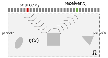
Figure 7: Illustration of a simple seismic imaging setting. The sources and receivers are located near the surface level (top) of the domain $\Omega$. The scatterer field $\eta(x)$ is assumed to be well-separated from the sources and the receivers.

Using the background velocity field $c_{0}(x)$, we first introduce the background Helmholtz operator $L_{0}=-\Delta-\omega^{2}/c_{0}(x)^{2}$. For each source $s$, we place a delta source at point $x_{s}$ and solve the the Helmholtz equation (in the differential imaging setting)

$$(L_{0}-\eta)(G_{0}(x,x_{s})+u^{s}(x))=0,$$ (3.1)

where $G_{0}=L_{0}^{-1}$ be the Green’s functions of the background Helmholtz operator $L_{0}$. The solution is recorded at points $x_{r}$ for $r\in R$ and the whole dataset is $d(s,r)\equiv u^{s}(x_{r})$. In order to understand better the relationship between $\eta(x)$ and $d(s,r)$, let us perform a perturbative analysis for small $\eta$. Expanding (3.1) gives rise to

$$(L_{0}u^{s})(x)=\eta(x)G_{0}(x,x_{s})+\ldots.$$

Solving this leads to

$$d(s,r)=u^{s}(r)=\int G_{0}(x_{r},x)G_{0}(x,x_{s})\eta(x)\,\mathrm{d}x+\ldots.$$

Again, we introduce $d_{1}(s,r)=\int G_{0}(x_{r},x)G_{0}(x,x_{s})\eta(x)\,\mathrm{d}x$ as the leading order linear term in terms of $\eta$.

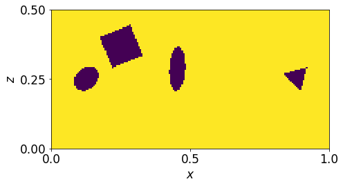
(a) $\eta(x)$

(b) $\Re(d(s,r))$

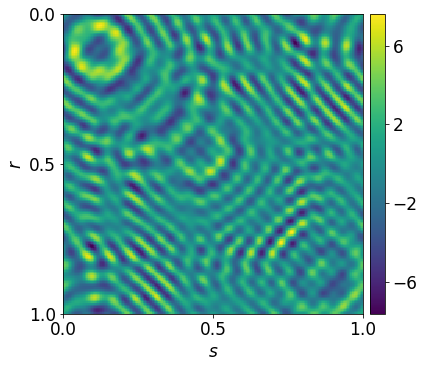
(c) $\Im(d(s,r))$

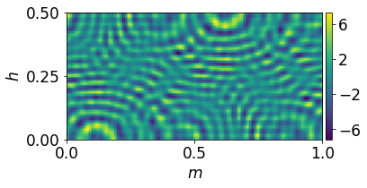
(d) $\Re(d(m,h))$

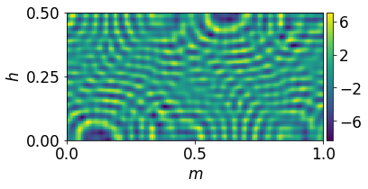
(e) $\Im(d(m,h))$

Figure 8: Visualization of the scatterer field $\eta$ and the measurement data $d$ for the seismic imaging. The upper figures are the scatterer and the real and imaginary part of the measurement data $d$, respectively. The lower two figures are the real and imaginary part of the measurement data after change of variable.

Figure 8 gives an example of the scatterer field and the measurement data. Notice that the strongest signal concentrates at the diagonal of the measurement data $d(s,r)$. Because of the periodicity in the horizontal direction, it is convenient to rotate the measurement data by a change of variables as

$$m=\frac{r+s}{2},h=\frac{r-s}{2},\quad\text{or equivalently}\quad r=m+h,s=m-h,$$ (3.2)

where all the variables $m,h,r,s$ are understood modulus $1$. With a bit abuse of notation, we recast the measurement data

$$d(m,h)\equiv d(s,r)|_{s=m-h,r=m+h},$$ (3.3)

and so does for $d_{1}(m,h)$. At the same time, by letting $x=(p,z)$ where $p$ is horizontal component of $x$ and $z$ is the depth component, we write $\eta(p,z)=\eta(x)$. Since $d_{1}(m,h)$ is linearly dependent on $\eta(p,z)$, there exists a kernel distribution $K(m,h,p,z)$ such that

$$d_{1}(m,h)=\int_{0}^{Z}\int_{0}^{1}K(m,h,p,z)\eta(p,z)\,\mathrm{d}z\,\mathrm{d}p.$$ (3.4)

One of the most common scenario in seismic imaging is that $c_{0}(x)$ only depends on the depth, i.e., $c_{0}(p,z)\equiv c_{0}(z)$. Note that in this scenario the whole problem is equivariant to translation in the horizontal direction. The system can be dramatically simplified due to the following proposition.

Proposition 2.

There exists a function $\kappa(h,z,\cdot)$ periodic in the last parameter such that $K(m,h,p,z)=\kappa(h,z,m-p)$ or equivalently,

$$d_{1}(m,h)=\int_{0}^{Z}\int_{0}^{1}\kappa(h,z,m-p)\eta(p,z)\,\mathrm{d}p\,\mathrm{d}z.$$ (3.5)

Proof.

Because of $c_{0}(p,z)=c_{0}(z)$ and the periodic boundary conditions in the horizontal direction, the Green’s function of the background Helmholtz operator $G_{0}$ is translation invariant on the horizontal direction, i.e., there exists a $g_{0}(\cdot,\cdot,\cdot)$ such that $G((x_{1},x_{2}),(y_{1},y_{2}))=g(x_{1}-y_{1},x_{2},y_{2})$. Therefore,

$$d_{1}(m,h) =\int_{0}^{Z}\int_{0}^{1}G_{0}((m+h,Z),(p,z))G_{0}((p,z),(m-h,Z))\eta(p,z)\,\mathrm{d}z\,\mathrm{d}p$$

$$=\int_{0}^{Z}\int_{0}^{1}g_{0}(m-p+h,Z,z)g_{0}(p-m+h,z,Z)\eta(p,z)\,\mathrm{d}z\,\mathrm{d}p.$$

Setting $\kappa(h,z,y)=g_{0}(y+h,Z,z)g_{0}(-y+h,z,Z)$ completes the proof. ∎

To discrete the problem, the scatterer $\eta(p,z)$ will be represented on a uniform mesh of $[0,1]\times[0,Z]$. With a slight abuse of notation, we shall use the same symbols to denote the discretization version of the continuous kernels and variables. The discrete version of 3.5 then becomes

$$d(m,h)\approx\sum_{z}\left(\kappa(h,z,\cdot)*\eta(\cdot,z)\right)(m).$$ (3.6)

3.2 Neural network and numerical examples

3.2.1 Neural network

Note that the key of the neural network architecture in Algorithm 2 for the far field pattern case is the convolution form in the angular direction in Proposition 1. For the seismic imaging case, Proposition 2 is the counterpart of Proposition 1. Since the argument in Section 2.2 remains valid for seismic imaging, the neural network architecture for seismic imaging is the same as that in Algorithm 2. However, the hyper-parameters are problem-dependent.

3.2.2 Experimental setup

In the experiment $Z=1/2$ and the domain $\Omega=[0,1]\times[0,Z]$ is discretized with a uniform Cartesian mesh with $192\times 96$ points with frequency $\omega=16$. The remaining setup of the numerical solution of the Helmholtz equation is same as that for the far field pattern problem. For the measurement, we also set the number of sources and receivers as $N_{s}=N_{r}=192$. The measurement data $d(s,r)$ is generated by solving the Helmholtz equation $N_{s}$ times by placing a delta function on each source point. For the change of variable of $(s,r)\to(m,h)$, linear interpolation is used for generating the data $d(m,h)$ from $d(s,r)$, with $N_{m}=192$ for $m\in[0,1)$ and $N_{h}=96$ for $h\in(0,1/2)$. In the actual simulation, we use both the real and imaginary part and concentrate them on the $h$ direction as the input.

3.2.3 Results

The numerical experiments here focus on the shape reconstruction setting, where $\eta$ are piecewise constant inclusions. Here, the scatterer field $\eta$ is assumed to be the sum of ${N_{\mathrm{shape}}}$ piecewise constant shapes. For each shape, it can be either triangle, square or ellipse, the orientation is uniformly random over the unit circle, the position is uniformly sampled in the $[0,1]\times[0.2,0.4]$, and the circumradius is sampled from the uniform distribution $\mathcal{U}(0.1,0.2)$. If the shape is ellipse, its width and height are sampled from the uniform distribution $\mathcal{U}(0.08,0.16)$ and $\mathcal{U}(0.04,0.8)$. It is also required that there is no intersection between any two shapes. We generate two datasets with ${N_{\mathrm{shape}}}=2$ and ${N_{\mathrm{shape}}}=4$ and each has $20,480$ samples $\{(\eta_{i},d_{i})\}$ with $16,384$ used for training and the remaining $4,096$ reserved for testing.

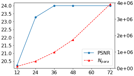
Figure 9: The test PSNR for seismic imaging for different channel numbers $c$ with ${N_{\mathrm{shape}}}=4$.

abcde${N_{\mathrm{shape}}}=4$
abcde${N_{\mathrm{shape}}}=2$

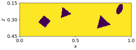
(a) reference

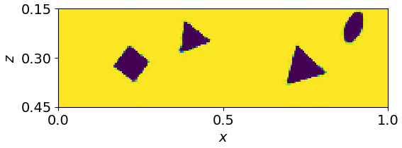
(b) $\eta^{\mathrm{NN}}$ with $\delta=0$

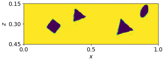
(c) $\eta^{\mathrm{NN}}$ with $\delta=10\%$

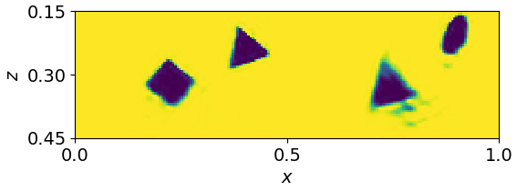
(d) $\eta^{\mathrm{NN}}$ with $\delta=100\%$

(e) reference

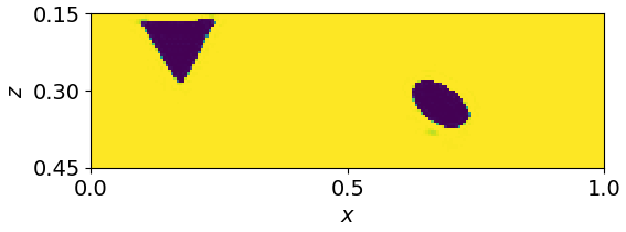
(f) $\eta^{\mathrm{NN}}$ with $\delta=0$

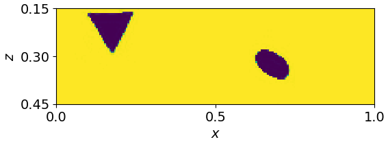
(g) $\eta^{\mathrm{NN}}$ with $\delta=10\%$

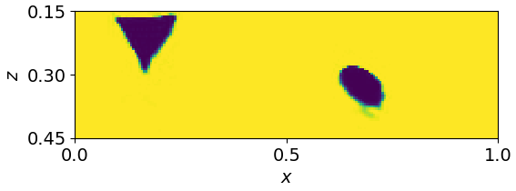
(h) $\eta^{\mathrm{NN}}$ with $\delta=100\%$

Figure 10: The seismic imaging problem. NN prediction of a sample with test data ${N_{\mathrm{shape}}}=4$ (the first two rows) or ${N_{\mathrm{shape}}}=2$ (the last two rows), at different noise level $\delta=0$, $10\%$ and $100\%$.

Test:n ${N_{\mathrm{shape}}}=4$
Train: ${N_{\mathrm{shape}}}=2$;
Test:n ${N_{\mathrm{shape}}}=2$
Train: ${N_{\mathrm{shape}}}=4$;

(a) reference

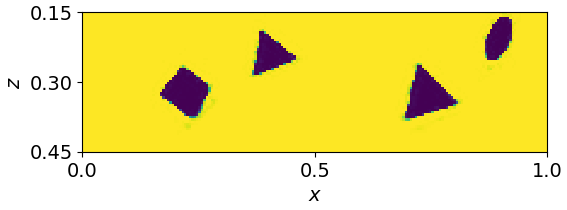
(b) $\eta^{\mathrm{NN}}$ with $\delta=0$

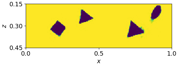
(c) $\eta^{\mathrm{NN}}$ with $\delta=10\%$

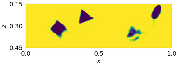
(d) $\eta^{\mathrm{NN}}$ with $\delta=100\%$

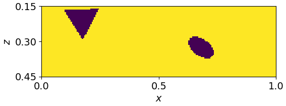
(e) reference

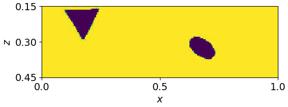
(f) $\eta^{\mathrm{NN}}$ with $\delta=0$

(g) $\eta^{\mathrm{NN}}$ with $\delta=10\%$

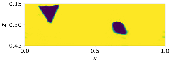
(h) $\eta^{\mathrm{NN}}$ with $\delta=100\%$

Figure 11: The seismic imaging problem: NN generalization test. In the top figures, the NN is trained by the data with ${N_{\mathrm{shape}}}=2$ at noise level $\delta=0$, $10\%$ or $100\%$ and tested by the data with ${N_{\mathrm{shape}}}=4$. In the bottom figures, the NN is trained by the data with ${N_{\mathrm{shape}}}=4$ and tested by the data with ${N_{\mathrm{shape}}}=2$.

The first study is about the choice of channel number $c$ in Algorithm 2. Figure 4 presents the test PSNR and the number of parameters, for different channel number $c$ on the dataset ${N_{\mathrm{shape}}}=4$. Similar to the far field pattern problem, as the channel number $c$ increases, the test PSNR first consistently increases and then saturates. Notice that the number of parameters of the neural network is $O(c^{2}\log(N_{\theta})N_{\mathrm{cnn}})$. The choice of $c=36$ is a reasonable balance between accuracy and efficiency and the total number of parameters is $981$K.

To model the uncertainty in the measurement data, the same method as the far field pattern problem is used to add noises to the measurement data. Figure 10 collects, for different noise level $\delta=0$, $10\%$, $100\%$, samples for ${N_{\mathrm{shape}}}=2$ and $4$, and Fig. 11 presents the generalization test of the proposed NN by training and testing on different datasets..

4 Discussions

This paper presents a neural network approach for the two typical problems of the inverse scattering: far field pattern and seismic imaging. The approach uses the NN to approximate the whole inverse map from the measurement data to the scatterer field, inspired by the perturbative analysis that indicates that the linearized forward map can be represented by a one-dimensional convolution with multiple channels. The analysis in this paper can also be extended to three-dimensional scattering problems. The analysis of seismic imaging can be easily extended to non-periodic boundary conditions by replacing the periodic padding in Algorithm 2 with zero padding.

References

- [1] M. Abadi et al. Tensorflow: A system for large-scale machine learning. In OSDI, volume 16, pages 265–283, 2016.
- [2] J. Adler and O. Öktem. Solving ill-posed inverse problems using iterative deep neural networks. Inverse Problems, 33(12):124007, 2017.
- [3] M. Araya-Polo, J. Jennings, A. Adler, and T. Dahlke. Deep-learning tomography. The Leading Edge, 37(1):58–66, 2018.
- [4] L. Bar and N. Sochen. Unsupervised deep learning algorithm for PDE-based forward and inverse problems. arXiv preprint arXiv:1904.05417, 2019.
- [5] J.-P. Berenger. Perfectly matched layer for the FDTD solution of wave-structure interaction problems. IEEE Transactions on antennas and propagation, 44(1):110–117, 1996.
- [6] J. Berg and K. Nyström. A unified deep artificial neural network approach to partial differential equations in complex geometries. Neurocomputing, 317:28–41, 2018.
- [7] G. Beylkin, R. Coifman, and V. Rokhlin. Fast wavelet transforms and numerical algorithms I. Communications on pure and applied mathematics, 44(2):141–183, 1991.
- [8] B. Borden. Mathematical problems in radar inverse scattering. Inverse Problems, 18(1):R1, 2001.
- [9] F. Cakoni, D. Colton, and P. Monk. The linear sampling method in inverse electromagnetic scattering, volume 80. SIAM, 2011.
- [10] G. Carleo and M. Troyer. Solving the quantum many-body problem with artificial neural networks. Science, 355(6325):602–606, 2017.
- [11] M. Cheney. The linear sampling method and the music algorithm. Inverse problems, 17(4):591, 2001.
- [12] F. Chollet et al. Keras. https://keras.io, 2015.
- [13] D. Colton and R. Kress. Looking back on inverse scattering theory. SIAM Review, 60(4):779–807, 2018.
- [14] D. L. Colton, R. Kress, and R. Kress. Inverse acoustic and electromagnetic scattering theory, volume 93. Springer, 1998.
- [15] G. Cybenko. Approximation by superpositions of a sigmoidal function. Mathematics of control, signals and systems, 2(4):303–314, 1989.
- [16] T. Dozat. Incorporating Nesterov momentum into adam. International Conference on Learning Representations, 2016.
- [17] W. E and B. Yu. The deep Ritz method: A deep learning-based numerical algorithm for solving variational problems. Communications in Mathematics and Statistics, 6(1):1–12, 2018.
- [18] B. Engquist and L. Ying. Fast directional algorithms for the Helmholtz kernel. Journal of Computational and Applied Mathematics, 234(6):1851–1859, 2010.
- [19] B. Engquist and L. Ying. Sweeping preconditioner for the Helmholtz equation: hierarchical matrix representation. Communications on pure and applied mathematics, 64(5):697–735, 2011.
- [20] B. Engquist and L. Ying. Sweeping preconditioner for the Helmholtz equation: moving perfectly matched layers. Multiscale Modeling & Simulation, 9(2):686–710, 2011.
- [21] Y. A. Erlangga. Advances in iterative methods and preconditioners for the Helmholtz equation. Archives of Computational Methods in Engineering, 15(1):37–66, 2008.
- [22] O. G. Ernst and M. J. Gander. Why it is difficult to solve Helmholtz problems with classical iterative methods. In Numerical analysis of multiscale problems, pages 325–363. Springer, 2012.
- [23] Y. Fan, C. O. Bohorquez, and L. Ying. BCR-Net: a neural network based on the nonstandard wavelet form. Journal of Computational Physics, 384:1–15, 2019.
- [24] Y. Fan, J. Feliu-Fabà, L. Lin, L. Ying, and L. Zepeda-Núñez. A multiscale neural network based on hierarchical nested bases. Research in the Mathematical Sciences, 6(2):21, 2019.
- [25] Y. Fan, L. Lin, L. Ying, and L. Zepeda-Núñez. A multiscale neural network based on hierarchical matrices. arXiv preprint arXiv:1807.01883, 2018.
- [26] Y. Fan and L. Ying. Solving electrical impedance tomography with deep learning. arXiv preprint arXiv:1906.03944, 2019.
- [27] Y. Fan and L. Ying. Solving optical tomography with deep learning. arXiv preprint arXiv:1910.04756, 2019.
- [28] J. Feliu-Faba, Y. Fan, and L. Ying. Meta-learning pseudo-differential operators with deep neural networks. arXiv preprint arXiv:1906.06782, 2019.
- [29] M. J. Gander and F. Nataf. AILU for Helmholtz problems: a new preconditioner based on the analytic parabolic factorization. Journal of Computational Acoustics, 9(04):1499–1506, 2001.
- [30] X. Glorot and Y. Bengio. Understanding the difficulty of training deep feedforward neural networks. In Proceedings of the thirteenth international conference on artificial intelligence and statistics, pages 249–256, 2010.
- [31] I. Goodfellow, Y. Bengio, A. Courville, and Y. Bengio. Deep learning, volume 1. MIT press Cambridge, 2016.
- [32] C. Greene, P. Wiebe, J. Burczynski, and M. Youngbluth. Acoustical detection of high-density krill demersal layers in the submarine canyons off georges bank. Science, 241(4863):359–361, 1988.
- [33] J. Han, A. Jentzen, and W. E. Solving high-dimensional partial differential equations using deep learning. Proceedings of the National Academy of Sciences, 115(34):8505–8510, 2018.
- [34] J. Han, L. Zhang, R. Car, and W. E. Deep potential: A general representation of a many-body potential energy surface. Communications in Computational Physics, 23(3):629–639, 2018.
- [35] T. Henriksson, N. Joachimowicz, C. Conessa, and J.-C. Bolomey. Quantitative microwave imaging for breast cancer detection using a planar 2.45 ghz system. IEEE Transactions on Instrumentation and Measurement, 59(10):2691–2699, 2010.
- [36] G. Hinton, L. Deng, D. Yu, G. E. Dahl, A. r. Mohamed, N. Jaitly, A. Senior, V. Vanhoucke, P. Nguyen, T. N. Sainath, and B. Kingsbury. Deep neural networks for acoustic modeling in speech recognition: The shared views of four research groups. IEEE Signal Processing Magazine, 29(6):82–97, 2012.
- [37] S. R. H. Hoole. Artificial neural networks in the solution of inverse electromagnetic field problems. IEEE transactions on Magnetics, 29(2):1931–1934, 1993.
- [38] T. Hulme, A. Haines, and J. Yu. General elastic wave scattering problems using an impedance operator approach-ii. two-dimensional isotropic validation and examples. Geophysical Journal International, 159(2):658–666, 2004.
- [39] M. I. Hussein, M. J. Leamy, and M. Ruzzene. Dynamics of phononic materials and structures: Historical origins, recent progress, and future outlook. Applied Mechanics Reviews, 66(4):040802, 2014.
- [40] H. Kabir, Y. Wang, M. Yu, and Q.-J. Zhang. Neural network inverse modeling and applications to microwave filter design. IEEE Transactions on Microwave Theory and Techniques, 56(4):867–879, 2008.
- [41] Y. Khoo, J. Lu, and L. Ying. Solving parametric PDE problems with artificial neural networks. arXiv preprint arXiv:1707.03351, 2017.
- [42] Y. Khoo, J. Lu, and L. Ying. Solving for high-dimensional committor functions using artificial neural networks. Research in the Mathematical Sciences, 6(1):1, 2019.
- [43] Y. Khoo and L. Ying. SwitchNet: a neural network model for forward and inverse scattering problems. arXiv preprint arXiv:1810.09675, 2018.
- [44] A. Kirsch. Factorization of the far-field operator for the inhomogeneous medium case and an application in inverse scattering theory. Inverse problems, 15(2):413, 1999.
- [45] A. Kirsch and N. Grinberg. The factorization method for inverse problems, volume 36. Oxford University Press, 2008.
- [46] A. Krizhevsky, I. Sutskever, and G. E. Hinton. ImageNet classification with deep convolutional neural networks. In Proceedings of the 25th International Conference on Neural Information Processing Systems - Volume 1, NIPS’12, pages 1097–1105, USA, 2012. Curran Associates Inc.
- [47] G. Kutyniok, P. Petersen, M. Raslan, and R. Schneider. A theoretical analysis of deep neural networks and parametric PDEs. arXiv preprint arXiv:1904.00377, 2019.
- [48] Y. LeCun, Y. Bengio, and G. Hinton. Deep learning. Nature, 521(436), 2015.
- [49] M. K. K. Leung, H. Y. Xiong, L. J. Lee, and B. J. Frey. Deep learning of the tissue-regulated splicing code. Bioinformatics, 30(12):i121–i129, 2014.
- [50] Y. Li, J. Lu, and A. Mao. Variational training of neural network approximations of solution maps for physical models. arXiv preprint arXiv:1905.02789, 2019.
- [51] F. Liu and L. Ying. Recursive sweeping preconditioner for the three-dimensional Helmholtz equation. SIAM Journal on Scientific Computing, 38(2):A814–A832, 2016.
- [52] Z. Long, Y. Lu, X. Ma, and B. Dong. PDE-net: Learning PDEs from data. In J. Dy and A. Krause, editors, Proceedings of the 35th International Conference on Machine Learning, volume 80 of Proceedings of Machine Learning Research, pages 3208–3216, Stockholmsmässan, Stockholm Sweden, 10–15 Jul 2018. PMLR.
- [53] A. Lucas, M. Iliadis, R. Molina, and A. K. Katsaggelos. Using deep neural networks for inverse problems in imaging: beyond analytical methods. IEEE Signal Processing Magazine, 35(1):20–36, 2018.
- [54] J. Ma, R. P. Sheridan, A. Liaw, G. E. Dahl, and V. Svetnik. Deep neural nets as a method for quantitative structure-activity relationships. Journal of Chemical Information and Modeling, 55(2):263–274, 2015.
- [55] P. Mora. Nonlinear two-dimensional elastic inversion of multioffset seismic data. Geophysics, 52(9):1211–1228, 1987.
- [56] S. J. Norton and M. Linzer. Ultrasonic reflectivity tomography: reconstruction with circular transducer arrays. Ultrasonic imaging, 1(2):154–184, 1979.
- [57] A. Palermo, S. Krödel, A. Marzani, and C. Daraio. Engineered metabarrier as shield from seismic surface waves. Scientific reports, 6:39356, 2016.
- [58] M. Raissi and G. E. Karniadakis. Hidden physics models: Machine learning of nonlinear partial differential equations. Journal of Computational Physics, 357:125 – 141, 2018.
- [59] M. Raissi, P. Perdikaris, and G. E. Karniadakis. Physics-informed neural networks: A deep learning framework for solving forward and inverse problems involving nonlinear partial differential equations. Journal of Computational Physics, 378:686–707, 2019.
- [60] K. Rudd and S. Ferrari. A constrained integration (CINT) approach to solving partial differential equations using artificial neural networks. Neurocomputing, 155:277–285, 2015.
- [61] J. Schmidhuber. Deep learning in neural networks: An overview. Neural Networks, 61:85–117, 2015.
- [62] I. Sutskever, O. Vinyals, and Q. V. Le. Sequence to sequence learning with neural networks. In Z. Ghahramani, M. Welling, C. Cortes, N. D. Lawrence, and K. Q. Weinberger, editors, Advances in Neural Information Processing Systems 27, pages 3104–3112. Curran Associates, Inc., 2014.
- [63] C. Tan, S. Lv, F. Dong, and M. Takei. Image reconstruction based on convolutional neural network for electrical resistance tomography. IEEE Sensors Journal, 19(1):196–204, 2018.
- [64] D. Verschuur and A. Berkhout. Estimation of multiple scattering by iterative inversion, part ii: Practical aspects and examples. Geophysics, 62(5):1596–1611, 1997.
- [65] A. B. Weglein, F. V. Araújo, P. M. Carvalho, R. H. Stolt, K. H. Matson, R. T. Coates, D. Corrigan, D. J. Foster, S. A. Shaw, and H. Zhang. Inverse scattering series and seismic exploration. Inverse problems, 19(6):R27, 2003.