Kinetics of Many-Body Reservoir Engineering

Abstract

Recent advances illustrate the power of reservoir engineering in applications to many-body systems, such as quantum simulators based on superconducting circuits. We present a framework based on kinetic equations and noise spectra that can be used to understand both the transient and long-time behavior of many particles coupled to an engineered reservoir in a number-conserving way. For the example of a bosonic array, we show that the non-equilibrium steady state can be expressed, in a wide parameter regime, in terms of a modified Bose-Einstein distribution with an energy-dependent temperature.

Introduction — Reservoir engineering Poyatos et al. (1996); Plenio and Huelga (2002); Kapit (2017) is used to deliberately generate some desired dissipative dynamics, as demonstrated in a variety of platforms: atoms Krauter et al. (2011), superconducting circuits Murch et al. (2012); Shankar et al. (2013); Leghtas et al. (2015), ion traps Barreiro et al. (2011); Lin et al. (2013); Kienzler et al. (2015), and optomechanics Wollman et al. (2015); Pirkkalainen et al. (2015). In the future, it could become particularly useful for controlling quantum many-body systems, as theoretically proposed in several works (see, e.g., Refs.  Diehl et al. (2008); Verstraete et al. (2009); Cho et al. (2011); Quijandría et al. (2013); Kapit et al. (2014); Reiter et al. (2016)).

First experimental realizations of many-body reservoir engineering are starting to appear: it has been used to stabilize a circuit QED based Mott insulator in a 1D chain of eight transmon qubits against photon losses Ma et al. (2019) as well as to dissipatively prepare quantum states in a three-transmon array Hacohen-Gourgy et al. (2015). In that way, reservoir engineering contributes to the implementation of quantum simulators, especially in cases where the naturally available dissipation would not drive the system to the right many-body ground state.

In this context, one very important scenario concerns the case where the coupling to the reservoir conserves the total number of particles Hacohen-Gourgy et al. (2015). Only then is it possible to cool without ending up in the vacuum state. Here, we are interested in providing a general framework to quantitatively describe the kinetics of many particles being scattered among states thanks to the (weak) interaction with an arbitrary non-equilibrium reservoir. The non-equilibrium nature is significant: even the steady-state distribution will depend on details of the interaction and of the reservoir noise spectrum, in contrast to the case of a thermal heat bath encountered, e.g., in certain approaches on particle-conserving photon equilibration Klaers et al. (2010); Schmitt et al. (2014); Hafezi et al. (2015).

We will introduce a perturbative approach to derive the steady-state distribution in momentum space. For the bosonic case treated here, this turns out to be a “deformed” Bose-Einstein distribution with an energy-dependent effective temperature. Illustrating the general theory in the specific case of a linear array of (harmonic) bosonic modes, we furthermore observe features such as negative-temperature states and prominent accumulation of particles at certain momenta during the time-evolution.

The physics we encounter is partially reminiscent of cavity optomechanics Aspelmeyer et al. (2014), except that we are now dealing with a many-particle system instead of a mechanical resonator. Furthermore, the coupling to that system has been engineered to preserve the number of excitations, somewhat analogous to the unconventional quadratic coupling encountered in some optomechanical systems.

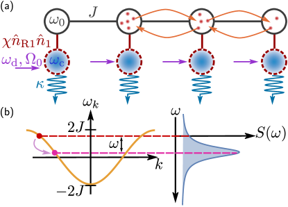
Figure 1: (Color Online) (a) Schematic representation of an array of bosonic modes, where each site experiences density-density coupling to a non-equilibrium reservoir (a driven, lossy cavity). (b) A particle at energy $\omega_{1}$ is scattered to a state of energy $\omega_{2}<\omega_{1}$ by emitting a photon into the reservoir. The rate at which particles scatter is proportional to the noise spectrum $S(\omega)$ of the reservoir.

Model— For concreteness we focus on bosons in a 1D array of modes with nearest-neighbor hopping. This physical situation can be realized, e.g., using linear elements of the superconducting circuits toolbox (capacitively coupled cavities). Each mode is further coupled to a lossy driven cavity via a density-density interaction [see Fig. 1 (a)]. The driven, lossy cavities will act as an engineered non-equilibrium reservoir that mediates transitions between the eigenstates of the array while simultaneously conserving the number of excitations; this ensures a well-defined chemical potential. We note that this type of coupling between system and reservoir can be achieved, e.g., via the anharmonic transmon terms when considering a single cavity coupled dispersively to an array of transmons. That was realized in Ref. Hacohen-Gourgy et al. (2015), using the reservoir to cool a Bose-Hubbard chain in the atomic limit, i.e., a three-site chain with at most two excitations. An alternative implementation would be an optomechanical array consisting of a chain of mechanical modes, each of which is coupled quadratically Sankey et al. (2010) to a driven cavity.

The Hamiltonian describing the system is given by

$$\hat{H}(t)=\hat{H}_{\mathrm{array}}+\hat{H}_{\mathrm{int}}+\hat{H}_{\mathrm{cav}}+\hat{H}_{\mathrm{drive}}(t),$$ (1)

where $\hat{H}_{\mathrm{array}}=\omega_{0}\sum_{j=1}^{L}\hat{b}_{j}^{\dagger}\hat{b}_{j}+J\sum_{j=1}^{L-1}(\hat{b}_{j+1}^{\dagger}\hat{b}_{j}+\mathrm{H.c.})$ with $\omega_{0}$ the frequency of the modes, $J$ the hopping strength, and $\hat{b}_{j}$ the annihilation operator of mode $j$. For the lossy cavities, the Hamiltonian is $\hat{H}_{\mathrm{cav}}=\omega_{\mathrm{c}}\sum_{j}\hat{a}^{\dagger}_{j}\hat{a}_{j}$, with $\omega_{\mathrm{c}}$ the frequency, and $\hat{a}_{j}$ the annihilation operator of a photon. Most importantly, we assume a density-density coupling between the array and the reservoir, of the form $\hat{H}_{\mathrm{int}}=\chi\sum_{j}\hat{a}^{\dagger}_{j}\hat{a}_{j}\hat{b}_{j}^{\dagger}\hat{b}_{j}$, with $\chi$ the coupling constant. As we show later, such a coupling allows one to cool the array while conserving the initial number of excitations present in the system. Alternatively, one can consider a situation where only the first site of the array is coupled to a driven reservoir. This setting leads qualitatively to the same cooling dynamics. However, the situation studied here presents the advantage of being homogeneous, having a well-defined thermodynamic limit, and the cooling power scaling with the length of the array. Finally, the classical drive on the reservoir cavity is given by $\hat{H}_{\mathrm{drive}}=\Omega_{0}\sum_{j}\exp(-i\omega_{\mathrm{d}}t)\hat{a}^{\dagger}_{j}+\mathrm{H.c.}$, with $\omega_{\mathrm{d}}$ the driving frequency and $\Omega_{0}$ the amplitude of the driving field.

The cooling dynamics of the array is best understood by diagonalizing $\hat{H}_{\mathrm{array}}$ and switching to a frame rotating at the drive frequency $\omega_{\mathrm{d}}$. To diagonalize the Hamiltonian of the array, we introduce the mode operators $\hat{\beta}_{k}$ defined via the relation $\hat{b}_{j}=\sum_{k}\varphi_{k}(j)\hat{\beta}_{k}$ where $\varphi_{k}(j)$ is the mode function determined via the boundary conditions of the problem (periodic or open). Then the interaction Hamiltonian is given by

$$\hat{H}_{\mathrm{int,\mathrm{R}}}=\chi\sum_{j,k,k^{\prime}}\varphi_{j}^{\ast}(k)\varphi_{j}(k^{\prime})\hat{a}_{j}^{\dagger}\hat{a}_{j}\hat{\beta}_{k}^{\dagger}\hat{\beta}_{k^{\prime}},$$ (2)

from which one sees that a transition from mode $k$ to $k^{\prime}$ is possible without exchanging particles with the reservoir. We note that for a finite-size system the wave vector $k$ has a discrete set of values, which are different for open and periodic boundary conditions.

To understand how such an interaction can give rise to cooling dynamics, it is useful to displace the reservoir field, i.e. $\hat{a}_{j}\to a_{0}+\hat{d}_{j}$, where $a_{0}$ is the classical amplitude of the field and the operator $\hat{d}_{j}$ describes the quantum noise affecting reservoir $j$ Marquardt et al. (2007); Clerk et al. (2010). Here, we neglect the fast transient dynamics and consider the reservoir to be in the steady state. This leads to $a_{0}=i\Omega_{0}/(i\Delta-\kappa/2)$ with $\kappa$ the energy decay rate. In the displaced frame the Hamiltonian of the system is

$$\hat{H}_{\mathrm{eff}} =\sum_{k}\omega_{k}\hat{\beta}_{k}^{\dagger}\hat{\beta}_{k}-\Delta\sum_{j=1}^{L}\hat{d}^{\dagger}_{j}\hat{d}_{j}+\chi\sum_{j,k,k^{\prime}}\varphi_{j}^{\ast}(k)\varphi_{j}(k^{\prime})$$ (3)

$$\phantom{={}}\times\left(\left|a_{0}\right|^{2}+a_{0}^{\ast}\hat{d}_{j}+a_{0}\hat{d}_{j}^{\dagger}+\hat{d}_{j}^{\dagger}\hat{d}_{j}\right)\hat{\beta}_{k}^{\dagger}\hat{\beta}_{k^{\prime}},$$

where $\omega_{k}=\omega_{0}+2J\cos(k)$ and $\Delta=\omega_{\mathrm{d}}-\omega_{\mathrm{c}}$ is the detuning between the reservoir cavity and the drive. Using Eq. (3) one can derive Golden rule rates describing transitions from mode $k$ to $k^{\prime}$, which generalizes optomechanical cooling ideas Marquardt et al. (2007); Clerk et al. (2010) to the many-body case,

$$\Gamma_{k\to k^{\prime}}=\gamma\chi^{2}S(\omega_{kk^{\prime}})n_{k}(n_{k^{\prime}}+1).$$ (4)

We introduce the power spectrum of the non-equilibrium reservoir noise, $S(\omega)$ $=$ $\left|a_{0}\right|^{2}\int_{-\infty}^{\infty}\mathop{}\!\mathrm{d}t\exp(i\omega t)\langle\hat{d}(t)\hat{d}^{\dagger}(0)\rangle$ $=$ $\left|a_{0}\right|^{2}\kappa/[(\omega+\Delta)^{2}+(\kappa/2)^{2}]$ [moreover, $\omega_{kk^{\prime}}=\omega_{k}-\omega_{k^{\prime}}$ and $\gamma=\sum_{i,j}\varphi_{i}^{\ast}(k)\varphi_{i}^{\ast}(k^{\prime})\varphi_{j}(k)\varphi_{j}(k^{\prime})$].

Now we are in a position to describe the cooling dynamics of the array, by formulating a set of coupled kinetic equations that describe the evolution of the average occupation of the eigenmodes of the array:

$$\dot{n}(\omega_{k},t)=\sum_{k^{\prime}\neq k}\left[\Gamma_{k^{\prime}\to k}(t)-\Gamma_{k\to k^{\prime}}(t)\right]$$ (5)

with $n(\omega_{k},t)=\langle\hat{\beta}_{k}^{\dagger}(t)\hat{\beta}_{k}(t)\rangle$. In the presence of weak interactions between particles, one would have to supplement Eq. (5) by addition of two-particle scattering terms Jaksch et al. (1997).

As it can be seen from Eq. (4), the sign of the detuning $\Delta$ determines whether the noise $S(\omega)$ [see Eq. (4)] peaks at either negative ($\Delta>0$) or positive ($\Delta<0$) frequency. As a consequence, by choosing the detuning $\Delta$ to be negative and assuming $\omega_{k}>\omega_{k^{\prime}}$, we have $\Gamma_{k\to k^{\prime}}>\Gamma_{k^{\prime}\to k}$ in Eq. (5). This corresponds to particles in high-energy modes being preferentially scattered into low-energy modes by having the reservoir absorb the excess of energy, leading to cooling. The reverse situation, with positive detuning $\Delta$, means the noise pumps energy incoherently into the array, scattering particles to higher energies. Another property of Eq. (4) that influences the dynamics described by Eq. (5) is the Bose enhancement factor; the rate at which a boson is scattered to a state with occupation $n$ is enhanced by a factor $n+1$.

Results — In the long-time limit, the system approaches a steady-state distribution. In general, this does not correspond to any thermal equilibrium distribution, as it can be seen in our numerical results [see Fig. 2 (a)] obtained on the basis of Eq. (5). An important aim in any non-equilibrium scenario is to characterize the resulting steady-state distributions.

First insights can be obtained by recalling that even for a noise source that is not in thermal equilibrium one can always define an effective temperature associated to a single transition frequency by using the Stokes relation $S(\omega)/S(-\omega)=\exp[\beta_{\mathrm{eff}}\omega]$ (or, alternatively, $\tanh[\beta_{\mathrm{eff}}\omega/2]=[S(\omega)-S(-\omega)]/[S(\omega)+S(-\omega)]$ Clerk et al. (2010)). In the limit where $\Delta^{2}+(\kappa/2)^{2}\gg\omega^{2}$ we can expand $S(\pm\omega)$ in powers of $1/[\Delta^{2}+(\kappa/2)^{2}]$. We also expand $\tanh[\beta_{\mathrm{eff}}\omega/2]$ around $\beta_{\mathrm{eff}}\omega\to 0$. Then, we find that the effective inverse temperature for a single transition frequency is given by

$$\beta_{\mathrm{eff}}(\omega)=\beta_{0}\left[1+\frac{\beta_{0}}{12\Delta}\left(3+\beta_{0}\Delta\right)\omega^{2}\right]+\mathcal{O}(\omega^{4})$$ (6)

where we defined the equilibrium temperature $\beta_{0}=-4\Delta/[\Delta^{2}+(\kappa/2)^{2}]$. In the limit $\Delta\to\infty$ or $\kappa\to\infty$, Eq. (6) shows that all transitions have the same temperature $\beta_{0}$. In this limit, the reservoir effectively acts as a thermal reservoir and we expect the steady state to be described by Bose-Einstein statistics with an inverse temperature $\beta_{0}$ and a chemical potential $\mu$: $n_{\mathrm{BE}}(\omega_{k})=[\exp\left[\beta_{0}(\omega_{k}-\mu)\right]-1]^{-1}$.

We will now demonstrate that, in the vicinity of this limiting case, the steady-state distribution can be understood as a certain deformed version of the Bose-Einstein distribution; in other words we look for a description in terms of small corrections around the equilibrium statistics. To do so, we turn to a perturbative solution of Eq. (5).

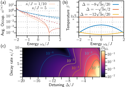
Figure 2: (Color Online) (a) Numerically observed steady-state distribution from Eq. (5) (solid thin lines), compared to perturbative solutions (solid thick lines) [see Eq. (8)], and Bose-Einstein statistics (dashed lines) ($\Delta=-3J$). (b) Effective energy-dependent inverse temperature $\beta(\omega_{k})$ of the modified Bose-Einstein distribution. (c) Kullback–Leibler divergence $D_{\mathrm{LK}}$ [see Eq. (10)] comparing the steady-state solution with the perturbative solution. In the limit $\beta_{0}J\ll 1$, the perturbative solution describes accurately the steady state of the system. For these simulations, we considered the experimentally relevant situation of open-boundary conditions and the parameters $L=100$, $N=50$, $\chi=J/1000$, and $\Omega_{0}=J/10$, unless specified otherwise.

The perturbation theory is best set up by considering the continuum limit of Eq. (5) for the steady state. We have

$$0 =\int_{-2J}^{2J}\mathop{}\!\mathrm{d}\omega_{k^{\prime}}D(\omega_{k^{\prime}})\left\{S(\omega)n(\omega_{k^{\prime}})[n(\omega_{k})+1]\right.$$ (7)

$$\phantom{==\int_{-2J}^{2J}\mathop{}\!\mathrm{d}\omega_{k^{\prime}}}\left.-S(-\omega)n(\omega_{k})[n(\omega_{k^{\prime}})+1]\right\},$$

with $\omega_{k^{\prime}}=\omega_{k}+\omega$ [see Fig. 1 (b)]. Here we introduced the density of states (for the 1D array, $D(\omega)=[{2\pi J\sqrt{1-\left(\frac{\omega}{2J}\right)^{2}}}]^{-1}$ when $|\omega|\leq 2J$).

The idea of the perturbative treatment is to look for a series representation of the distribution $n(\omega_{k})$: $n(\omega_{k})=\sum_{i}n_{i}(\omega_{k})$, with $n_{i}\propto(\beta_{0}\omega_{k})^{i}$ (see supplemental information for more details). We find

$$n(\omega_{k}) =n_{\mathrm{BE}}(\omega_{k})\left\{1-\exp[\beta_{0}(\omega_{k}-\mu)]n_{\mathrm{BE}}(\omega_{k})\times\vphantom{\frac{\beta_{0}^{2}}{36\Delta}}\right.$$ (8)

$$\phantom{={}}\left.\left[\frac{\beta_{0}^{2}}{36\Delta}(3+\beta_{0}\Delta)(\omega_{k}^{2}+18J^{2})\omega_{k}-\exp(-\beta_{0}\mu)c\right]\right\},$$

where $n_{\mathrm{BE}}(\omega_{k})$ is the Bose-Einstein statistics and $c$ is a constant of integration. We can fix both $\mu$ and $c$ in Eq. (8) by enforcing particle number conservation, $\sum_{k}n(\omega_{k})=N$; we first obtain $\mu$ by imposing normalization for $n_{\mathrm{BE}}$ and then extract $c$ from the same condition applied to the next order.

When we compare Eq. (8) to a generalized Bose-Einstein statistics with an energy-dependent inverse temperature (setting $\beta_{0}\to\beta(\omega_{k})$), we conclude, to leading order:

$$\beta(\omega_{k})=\beta_{0}\left[1+\frac{\beta_{0}}{36\Delta}(3+\beta_{0}\Delta)(\omega_{k}^{2}+18J^{2})\right].$$ (9)

In Fig. 2 (a), we display the inverse temperature as a function of energy. One can see that the curvature depends on the ratio between the detuning $\Delta$ and the decay rate $\kappa$. We note that Eq. (9) in addition to reduce to $\beta_{0}$ for a small expansion parameter [see Eq. (6)] also reduces to $\beta_{0}$ at the special point $\Delta=-\sqrt{3}\kappa/2$.

To assess the accuracy of our perturbative solution, we quantify its distance from the true steady-state solution of Eq. (8). We employ the Kullback–Leibler divergence Kullback and Leibler (1951) (relative entropy)

$$D_{\mathrm{KL}}\left(p^{(\infty)}\parallel p\right)=\sum_{k}\frac{n^{(\infty)}(\omega_{k})}{N}\log\left[\frac{n^{(\infty)}(\omega_{k})}{n(\omega_{k})}\right],$$ (10)

which describes the amount of information lost when approximating one distribution by another. Here, we expressed our perturbative solution in terms of the normalized density $p(\omega_{k})=n(\omega_{k})/N$ [with $N$ the total number of particles and $n(\omega_{k})$ given by Eq. (8)] and compare it to the steady-state distribution $p^{(\infty)}(\omega_{k})=n^{(\infty)}(\omega_{k})/N$.

Figure 2 (c) shows the Kullback–Leibler divergence as a function of detuning and decay rate. The numerical results were obtained by time-evolving the kinetic equations until the system settles into the steady state.

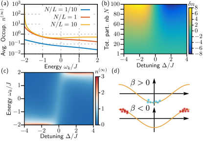
Figure 3: (Color Online) Bosonic distribution in momentum space (long-time limit). (a) Impact of the Bose enhancement factor ($\Delta=-J,\kappa=3J$). As the particle density increases, the low-energy levels become more occupied during the cooling dynamics. (b) Efficiency of ground state cooling. We plot the difference between the average occupation of the ground state and the highest excited state, $\delta n=n_{\mathrm{GS}}-n_{\mathrm{high}}$ ($\kappa=3J$). (c) Transition towards negative temperature. For blue detuning ($\Delta>0$), the system exhibits stable negative-temperatures steady states. (d) Schematic representation of states with positive and negative temperatures.

We observe the pertubative solution in Eq. (8) approximating the non-equilibrium steady state well in a wide range of parameters. The approximation becomes better, as expected, in the limit $\beta_{0}J\ll 1$ (for $\beta_{0}J\to 0$, the effective temperature becomes energy-independent, and Eq. (8) reduces back to the Bose-Einstein distribution). We stress that Eq. (8) is much closer to the real solution than the Bose-Einstein distribution itself; indeed, in a large parameter regime we have $D_{\mathrm{KL}}(p^{(\infty)}\parallel p_{\mathrm{BE}})/D_{\mathrm{KL}}(p^{(\infty)}\parallel p)\approx 10^{2}$ with $p_{\mathrm{BE}}=n_{\mathrm{BE}}/N$ (see supplemental material).

While we focussed on the specific case of a one-dimensional chain coupled to a non-equilibrium reservoir with a particular noise spectrum, our perturbative treatment is applicable to any spectrum and for non-interacting bosons in any dimension, in arbitrary potentials, with suitably modified mode functions and density of states. In all of these cases, it can serve to extract the steady-state non-equilibrium distribution brought about by reservoir-induced particle scattering.

Equation (8) represents our main analytical result. We now discuss some distinct properties of the non-equilibrium distribution.

In thermal equilibrium, detailed balance ensures that the Bose-Einstein distribution is independent of the density of states. This is no longer true here, out of equilibrium. As we show in Fig. 2 (b), signatures of the density of states (with its characteristic divergence at the band edge in 1D) can be observed when the noise spectrum itself [see Eq. (4)] is sufficiently narrow i.e, for $\kappa/J\ll 1$. In that case, prominent features (almost non-analytic) appear in the distribution at energies separated from the band edge by the detuning. These features are even more pronounced during the temporal dynamics (see below).

When deriving the kinetic equation [Eq. (4)], we pointed out the presence of the bosonic enhancement factors. The effects of such an enhancement can be observed when the particle density increases, particularly in the most strongly occupied regions of the band [see Fig. 3 (a)]. For red detuning, we obtain many-particle ground state cooling. To assess its efficiency, we plot in Fig. 3 (b) the difference between the occupation of the single-particle ground state and the highest excited state in the band, $\delta n=n_{\mathrm{high}}-n_{\mathrm{GS}}$. The bosonic enhancement serves to increase the efficiency of ground state cooling.

In stark contrast to optomechanics, where the spectrum of the mechanical resonator is unbounded, we are dealing with a physical system that possesses a bound (many-particle) spectrum. This has an important consequence: even for blue detuning ($\Delta>0$), and without any recourse to non-linear cavity dynamics, the system is still stable, as can be seen in Fig. 3 (c). In this “heating” regime, particles accumulate at the upper band edge. Such states can be described by a negative temperature [see Fig. 3 (d)]. Similar negative-temperature states were previously obtained using localized spin systems Purcell and Pound (1951); Oja and Lounasmaa (1997); Medley et al. (2011) and ultracold atoms trapped in optical lattices Braun et al. (2013). Creating stable negative states with optical lattices is challenging as it requires relatively complex state preparation. By contrast, here, one only needs to choose a positive detuning.

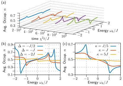
Figure 4: (Color Online) Time evolution. (a) Snapshots of the distribution showing the emergence of accumulation and depletion of particles at $\pm\Delta$ off the band edges ($\Delta=-3J,\kappa=J/10$). The steady-state distribution can be seen in Fig. 2 (a). (b) Detuning-dependence ($\chi^{2}t/J=10$, $\kappa=J/10$). (c) Impact of the decay rate $\kappa$.

Finally, we investigate the time-evolution. We are interested in describing the mechanism that leads to the accumulation and depletion of particles in the distribution, as shown in Fig. 4. As we noted earlier, these features are present in the steady-state distribution [see Fig. 2 (b)], so we expect them to be generic also during the evolution. To consider the simplest possible situation, we assume the initial distribution to be uniform. Such a uniform distribution in $k$-space can be realized, e.g., by incoherently loading the whole array with bosons at constant density (or quenching from a Mott insulator). At early times, the incipient deviations from the uniform distribution can be obtained perturbatively:

$$\dot{n}(\omega_{k},t)=\gamma\chi^{2}n_{0}(n_{0}+1)\mkern-18.0mu\int\displaylimits_{-2J-\omega_{k}}^{2J-\omega_{k}}\mkern-18.0mu\mathop{}\!\mathrm{d}\omega D(\omega+\omega_{k})\left[S(\omega)-S(-\omega)\right],$$ (11)

where we have replaced $n(\omega_{k},t)$ by its initial uniform value $n_{0}$. The integral in Eq. (11) is maximal (or minimal) when the divergence of the density of states aligns with the maximum of the spectrum $S(\omega)$ [or $S(-\omega)$]. Physically, this translates into having a large incoming rate of particles for states with $\omega_{k}=2J+\Delta$ and a large outgoing rate for states with $\omega_{k}=-2J-\Delta$ (assuming $\Delta<0$). As a consequence, particles accumulate (deplete) at $\pm\Delta$ from the band edges [see Figs. 4 (b), and 4 (c)]. The accumulation of particles at $\omega_{k}=2J+\Delta$ can subsequently lead to another accumulation of particles at $\omega_{k}=2J+2\Delta$ [see Fig. 4 (b), $\Delta=-J/2$]. As emphasized already above for the steady state, observing these extra peaks in the distribution is contingent on having a narrow cavity spectrum, with $\kappa\ll|\Delta|,J$ [see Fig. 4 (c)]

In experimental implementations, two factors may come into play to distort the long-term dynamics from the idealized scenario - we mention them briefly, though a detailed study would be beyond the scope of the present work. First, there is the loss of array bosons at a constant rate (e.g. intrinsic cavity decay or mechanical dissipation). This will simply lead to an overall depletion of the total particle number $N(t)\sim e^{-\Gamma t}$ (i.e. the steady state will slowly evolve, due to the modification of bosonic enhancement factors). Second, if there are interactions between the bosons (e.g. attractive interactions for a chain of transmon qubits instead of linear cavities), these will lead to additional scattering that is compatible with ground-state cooling but will drive the distribution closer to thermal.

Conclusion — We have investigated the scattering kinetics of bosonic particles subject to what is probably the most widely used engineered reservoir, namely a driven lossy cavity. We have shown that the resulting non-equilibrium steady-state distribution can be perturbatively analyzed in a wide parameter regime and interpreted as a deformed Bose-Einstein distribution with an energy-dependent temperature. In this work, we have focussed on the illustrative case of a one-dimensional array, with each site coupled to a driven cavity. However, our treatment remains valid and we expect similar observations in general for non-equilibrium reservoirs coupled in a particle-conserving manner to arbitrary non-interacting many-body systems, i.e. in higher-dimensions, for arbitrary lattices and band structures, and also for fermionic systems, with straightforward modifications.

I Perturbation theory

In this section, we show in more details how we obtained Eq. (8) of the main text. We start from the equation giving the steady state in the continuum limit [see also Eq. (7) of the main text],

$$0=\int\displaylimits_{-2J}^{2J}\mathop{}\!\mathrm{d}\omega_{k^{\prime}}D(\omega_{k^{\prime}})\left\{S(\omega)n(\omega_{k^{\prime}})[n(\omega_{k})+1]-S(-\omega)n(\omega_{k})[n(\omega_{k^{\prime}})+1]\right\}.$$ (S1)

The first step consists in expanding both $S(\omega)$ and $S(-\omega)$ in powers of $\beta_{0}\omega$. We have

$$S(\omega) =\left|a_{0}\right|^{2}\frac{\kappa}{(\omega+\Delta)^{2}+\left(\frac{\kappa}{2}\right)^{2}}$$ (S2)

$$=\left|a_{0}\right|^{2}\frac{\kappa}{\Delta^{2}+\left(\frac{\kappa}{2}\right)^{2}}\frac{1}{1+\frac{4\Delta}{\Delta^{2}+\left(\frac{\kappa}{2}\right)^{2}}\frac{\omega}{2}\left(1+\frac{\omega}{2\Delta}\right)}$$

$$=\left|a_{0}\right|^{2}\frac{\kappa}{\Delta^{2}+\left(\frac{\kappa}{2}\right)^{2}}\frac{1}{1-\beta_{0}\frac{\omega}{2}\left(1+\frac{\omega}{2\Delta}\right)}$$

$$=\left|a_{0}\right|^{2}\frac{\kappa}{\Delta^{2}+\left(\frac{\kappa}{2}\right)^{2}}\sum_{l=0}^{\infty}\left[\frac{\beta_{0}}{2\omega}\left(1+\frac{\omega}{2\Delta}\right)\right]^{l}$$

and similarly we have

$$S(-\omega)=\left|a_{0}\right|^{2}\frac{\kappa}{\Delta^{2}+\left(\frac{\kappa}{2}\right)^{2}}\sum_{l=0}^{\infty}\left[-\frac{\beta_{0}}{2\omega}\left(1+\frac{\omega}{2\Delta}\right)\right]^{l}.$$ (S3)

We also expand $n(\omega_{k^{\prime}})=n(\omega_{k}+\omega)$ in a Taylor series around $\omega=0$, we have

$$n(\omega_{k}+\omega)=\sum_{l=0}^{\infty}\frac{n^{(l)}(\omega_{k})}{l!}\omega^{l},$$ (S4)

where $n^{(l)}$ denotes the $l$th derivate of $n(\omega_{j})$.

By replacing Eqs. (S2), (S3), and (S4) into Eq. (S1), we can carry out the integral over the density of states. We look for solutions of the resulting equation in the form of a series expansion

$$n(\omega_{k})=\sum_{l=0}^{\infty}n_{l}(\omega_{k}),$$ (S5)

where we assume that $n_{l}\propto(\beta_{0}\omega_{k})^{l}$.

By expanding Eqs. (S2), (S3), and (S4) to third order, i.e, up to $l=3$, we can find first order differential equations for $n_{l}$ with $l\in\{0,1,2\}$ by grouping together terms proportional to $(\beta_{0}\omega_{k})^{l}$. We note that we treat terms like $(\beta_{0}\omega_{k})\omega_{k}/\Delta$ as being higher order, i.e., for this particular example this term would be grouped together with terms scaling like $(\beta_{0}\omega_{k})^{2}$.

Collecting terms proportional to $\beta_{0}\omega_{k}$, we find that $n_{0}(\omega_{k})$ must obey the differential equation

$$n^{\prime}_{0}(\omega_{k})+\beta_{0}n_{0}(\omega_{k})[n_{0}(\omega_{k})+1]=0.$$ (S6)

The solution of Eq. (S7) is the Bose-Einstein statistics with temperature $\beta_{0}$,

$$n_{0}(\omega_{k})=\frac{1}{\exp\left[\beta_{0}(\omega_{k}-\mu)\right]-1},$$ (S7)

and the constant of integration $\mu$ is the chemical potential, which is fixed by requiring that $\sum_{k}n_{0}(\omega_{k})=N$

Collecting terms proportional to $(\beta_{0}\omega_{k})^{2}$, we find that $n_{1}(\omega_{k})$ must obey the differential equation

$$n^{\prime}_{1}(\omega_{k})+\beta_{0}n_{1}(\omega_{k})[n_{0}(\omega_{k})+1]=0,$$ (S8)

whose solution is

$$n_{1}(\omega_{k})=c_{1}\frac{\exp\left[\beta_{0}(\omega_{k}-2\mu)\right]}{\left\{\exp\left[\beta_{0}(\omega_{k}-\mu)\right]-1\right\}^{2}},$$ (S9)

with $c_{1}$ a constant of integration. To determine the constant $c_{1}$ we require that $\sum_{k}[n_{0}(\omega_{k})+n_{1}(\omega_{k})]=N$. Note that we have previously fixed $\mu$ by requiring that $\sum_{k}n_{0}(\omega_{k})=N$, which leads to $c_{1}=0$. We note that this procedure to find the constants of integration ensures that our solution always describes a distribution with $N$ particles at every order.

Finally, collecting terms proportional to $(\beta_{0}\omega_{k})^{3}$, we find that $n_{2}(\omega_{k})$ must obey the differential equation

$$n^{\prime}_{2}(\omega_{k})+\beta_{0}n_{2}(\omega_{k})[2n_{0}(\omega_{k})+1]+\frac{\beta_{0}^{2}(3+\beta_{0}\Delta)(6J^{2}+\omega_{k}^{2})}{12\Delta}n_{0}(\omega_{k})[n_{0}(\omega_{k})+1]=0.$$ (S10)

The solution of Eq. (S10) is

$$n_{2}(\omega_{k})=-\frac{\exp\left[\beta_{0}(\omega_{k}-\mu\right]}{\left\{\exp\left[\beta_{0}(\omega_{k}-\mu)\right]-1\right\}^{2}}\left[\frac{\beta_{0}^{2}}{36\Delta}(3+\beta_{0}\Delta)(18J^{2}+\omega_{k}^{2})\omega_{k}-\exp(\beta_{0}\mu)c_{2}\right],$$ (S11)

with $c_{2}$ the constant of integration which is once more determined by the condition $\sum_{k}[n_{0}(\omega_{k})+n_{2}(\omega_{k})]=N$.

Combining Eqs. (S7), (S9), and (S11) together with the result $c_{1}=0$ leads to Eq. (8) of the main text. We note that the latter equation can predict negative occupation numbers, but this only occurs outside of the perturbative regime where the theory is not valid anymore.

II Approximating the steady-state solution with the Bose-Einstein statistics

In this section we show that the third order perturbative solution is a better approximation of the steady-state solution than the leading order Bose-Einstein statistics. In Fig. S1 (a) we plot the Kullback–Leibler divergence between $p^{(\infty)}$ and $p_{\mathrm{BE}}$. We indicate by a white dashed line when $\beta(\omega_{k})=\beta_{0}$ [see Eq. (9)], i.e., $\Delta=-\sqrt{3}\kappa/2$. When this last condition is met, we have $n_{2}(\omega_{k})=0$ if $c_{2}=0$.

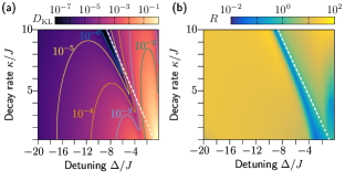
Figure S1: (Color Online) (a) Kullback–Leibler divergence comparing the steady-state solution with the Bose-Einstein statistics given by Eq. (S7). (b) Ratio between $D_{\mathrm{KL}}(p^{(\infty)}\parallel p_{\mathrm{BE}})$ and $D_{\mathrm{KL}}(p^{(\infty)}\parallel p)$. The white dashed line corresponds to $\Delta=-\sqrt{3}\kappa/2$ where the temperature $\beta(\omega_{k})$ is equal to $\beta_{0}$.

In Fig. S1 (b), we plot the ratio

$$R=\frac{D_{\mathrm{KL}}(p^{(\infty)}\parallel p_{\mathrm{BE}})}{D_{\mathrm{KL}}(p^{(\infty)}\parallel p)},$$ (S12)

which shows that the higher order perturbation approximates the steady-state solution more accurately than the leading order given by the Bose-Einstein statistics. We note, however, that in the close vicinity of $\Delta=-\sqrt{3}\kappa/2$, the leading order is more suitable to approximate the steady state.

References

- Poyatos et al. (1996) J. F. Poyatos, J. I. Cirac, and P. Zoller, Quantum reservoir engineering with laser cooled trapped ions, Phys. Rev. Lett. 77, 4728 (1996).
- Plenio and Huelga (2002) M. B. Plenio and S. F. Huelga, Entangled light from white noise, Phys. Rev. Lett. 88, 197901 (2002).
- Kapit (2017) E. Kapit, The upside of noise: engineered dissipation as a resource in superconducting circuits, Quantum Science and Technology 2, 033002 (2017).
- Krauter et al. (2011) H. Krauter, C. A. Muschik, K. Jensen, W. Wasilewski, J. M. Petersen, J. I. Cirac, and E. S. Polzik, Entanglement generated by dissipation and steady state entanglement of two macroscopic objects, Phys. Rev. Lett. 107, 080503 (2011).
- Murch et al. (2012) K. W. Murch, U. Vool, D. Zhou, S. J. Weber, S. M. Girvin, and I. Siddiqi, Cavity-assisted quantum bath engineering, Phys. Rev. Lett. 109, 183602 (2012).
- Shankar et al. (2013) S. Shankar, M. Hatridge, Z. Leghtas, K. M. Sliwa, A. Narla, U. Vool, S. M. Girvin, L. Frunzio, M. Mirrahimi, and M. H. Devoret, Autonomously stabilized entanglement between two superconducting quantum bits, Nature 504, 419 (2013).
- Leghtas et al. (2015) Z. Leghtas, S. Touzard, I. M. Pop, A. Kou, B. Vlastakis, A. Petrenko, K. M. Sliwa, A. Narla, S. Shankar, M. J. Hatridge, M. Reagor, L. Frunzio, R. J. Schoelkopf, M. Mirrahimi, and M. H. Devoret, Confining the state of light to a quantum manifold by engineered two-photon loss, Science 347, 853 (2015).
- Barreiro et al. (2011) J. T. Barreiro, M. Müller, P. Schindler, D. Nigg, T. Monz, M. Chwalla, M. Hennrich, C. F. Roos, P. Zoller, and R. Blatt, An open-system quantum simulator with trapped ions, Nature 470, 486 (2011).
- Lin et al. (2013) Y. Lin, J. P. Gaebler, F. Reiter, T. R. Tan, R. Bowler, A. S. Sørensen, D. Leibfried, and D. J. Wineland, Dissipative production of a maximally entangled steady state of two quantum bits, Nature 504, 415 (2013).
- Kienzler et al. (2015) D. Kienzler, H.-Y. Lo, B. Keitch, L. de Clercq, F. Leupold, F. Lindenfelser, M. Marinelli, V. Negnevitsky, and J. P. Home, Quantum harmonic oscillator state synthesis by reservoir engineering, Science 347, 53 (2015).
- Wollman et al. (2015) E. E. Wollman, C. U. Lei, A. J. Weinstein, J. Suh, A. Kronwald, F. Marquardt, A. A. Clerk, and K. C. Schwab, Quantum squeezing of motion in a mechanical resonator, Science 349, 952 (2015).
- Pirkkalainen et al. (2015) J.-M. Pirkkalainen, E. Damskägg, M. Brandt, F. Massel, and M. A. Sillanpää, Squeezing of quantum noise of motion in a micromechanical resonator, Phys. Rev. Lett. 115, 243601 (2015).
- Diehl et al. (2008) S. Diehl, A. Micheli, A. Kantian, B. Kraus, H. P. Büchler, and P. Zoller, Quantum states and phases in driven open quantum systems with cold atoms, Nature Physics 4, 878 (2008).
- Verstraete et al. (2009) F. Verstraete, M. M. Wolf, and J. Ignacio Cirac, Quantum computation and quantum-state engineering driven by dissipation, Nature Physics 5, 633 (2009).
- Cho et al. (2011) J. Cho, S. Bose, and M. S. Kim, Optical pumping into many-body entanglement, Phys. Rev. Lett. 106, 020504 (2011).
- Quijandría et al. (2013) F. Quijandría, D. Porras, J. J. García-Ripoll, and D. Zueco, Circuit qed bright source for chiral entangled light based on dissipation, Phys. Rev. Lett. 111, 073602 (2013).
- Kapit et al. (2014) E. Kapit, M. Hafezi, and S. H. Simon, Induced self-stabilization in fractional quantum hall states of light, Phys. Rev. X 4, 031039 (2014).
- Reiter et al. (2016) F. Reiter, D. Reeb, and A. S. Sørensen, Scalable dissipative preparation of many-body entanglement, Phys. Rev. Lett. 117, 040501 (2016).
- Ma et al. (2019) R. Ma, B. Saxberg, C. Owens, N. Leung, Y. Lu, J. Simon, and D. I. Schuster, A dissipatively stabilized mott insulator of photons, Nature 566, 51 (2019).
- Hacohen-Gourgy et al. (2015) S. Hacohen-Gourgy, V. V. Ramasesh, C. De Grandi, I. Siddiqi, and S. M. Girvin, Cooling and autonomous feedback in a bose-hubbard chain with attractive interactions, Phys. Rev. Lett. 115, 240501 (2015).
- Klaers et al. (2010) J. Klaers, J. Schmitt, F. Vewinger, and M. Weitz, Bose-einstein condensation of photons in an optical microcavity, Nature 468, 545 (2010).
- Schmitt et al. (2014) J. Schmitt, T. Damm, D. Dung, F. Vewinger, J. Klaers, and M. Weitz, Observation of grand-canonical number statistics in a photon bose-einstein condensate, Phys. Rev. Lett. 112, 030401 (2014).
- Hafezi et al. (2015) M. Hafezi, P. Adhikari, and J. M. Taylor, Chemical potential for light by parametric coupling, Phys. Rev. B 92, 174305 (2015).
- Aspelmeyer et al. (2014) M. Aspelmeyer, T. J. Kippenberg, and F. Marquardt, Cavity optomechanics, Rev. Mod. Phys. 86, 1391 (2014).
- Sankey et al. (2010) J. C. Sankey, C. Yang, B. M. Zwickl, A. M. Jayich, and J. G. E. Harris, Strong and tunable nonlinear optomechanical coupling in a low-loss system, Nature Physics 6, 707 (2010).
- Marquardt et al. (2007) F. Marquardt, J. P. Chen, A. A. Clerk, and S. M. Girvin, Quantum theory of cavity-assisted sideband cooling of mechanical motion, Phys. Rev. Lett. 99, 093902 (2007).
- Clerk et al. (2010) A. A. Clerk, M. H. Devoret, S. M. Girvin, F. Marquardt, and R. J. Schoelkopf, Introduction to quantum noise, measurement, and amplification, Rev. Mod. Phys. 82, 1155 (2010).
- Jaksch et al. (1997) D. Jaksch, C. W. Gardiner, and P. Zoller, Quantum kinetic theory. ii. simulation of the quantum boltzmann master equation, Phys. Rev. A 56, 575 (1997).
- Kullback and Leibler (1951) S. Kullback and R. A. Leibler, On information and sufficiency, Ann. Math. Statist. 22, 79 (1951).
- Purcell and Pound (1951) E. M. Purcell and R. V. Pound, A nuclear spin system at negative temperature, Phys. Rev. 81, 279 (1951).
- Oja and Lounasmaa (1997) A. S. Oja and O. V. Lounasmaa, Nuclear magnetic ordering in simple metals at positive and negative nanokelvin temperatures, Rev. Mod. Phys. 69, 1 (1997).
- Medley et al. (2011) P. Medley, D. M. Weld, H. Miyake, D. E. Pritchard, and W. Ketterle, Spin gradient demagnetization cooling of ultracold atoms, Phys. Rev. Lett. 106, 195301 (2011).
- Braun et al. (2013) S. Braun, J. P. Ronzheimer, M. Schreiber, S. S. Hodgman, T. Rom, I. Bloch, and U. Schneider, Negative absolute temperature for motional degrees of freedom, Science 339, 52 (2013).
Supplemental Material for