Excitons in Cu₂O - from Quantum Dots to Bulk Crystals and
Additional Boundary Conditions for Rydberg Exciton - Polaritons

Abstract

We propose schemes for calculation of optical functions of a semiconductor with Rydberg excitons for a wide interval of dimensions. We have started with a zero-dimensional structure (Quantum Dot), then going to one-dimensional (Quantum Wire), two-dimensional (Quantum Wells and Wide Quantum Wells) ending on 3-dimensional bulk crystals; our analytical fidings are illustrated numerically showing an agreement with avaliable experimental data. The calculations including excitons-polaritons are performed; the case of large number of polariton branches is discussed and obtained theoretical absorption spectra show good agreement with experimental data.

I Introduction

Since 2014 the Rydberg excitons (RE) in cuprous oxide, first observed by Kazimierczuk et al Kazimierczuk , have been subject of extensive research. Unusual properties of RE Hecktoeter_2017 ; Assmann_symmetry manifested in their interaction with external fields below Thewes ; Schoene ; FS95 ; Magnetoexcitons_2019 and above the gap energy FK in linear and nonlinear Walther ; Nonlinear regime have been studied, both experimentally Kazimierczuk ; FS96 ; Heckotter_plasma and theoretically Zielinska.PRB ; Zielinska.PRB.2016.b ; Zielinska.PRB.2016.c , the list being far from completeness.

In recent years, there has been a dedicated effort to describe the spectroscopic and optical properties of RE and several methods have been applied. Calculations based on the group theory have been used to obtain the dependence of the spectra on the geometry of external fields FS95 ; FS96 for RE up to $n=5$, while application of the mesoscopic Real Density Matrix Approach (RDMA) has turned out to be fruitful for description of optical function of semiconductor crystals including RE for the case of indirect interband transitions, as it was shown in the series of papers by S. Zielińska-Raczyńska et al. Zielinska.PRB ; Zielinska.PRB.2016.b ; Zielinska.PRB.2016.c This approach has turned out to be very flexible and general; it allows one to obtain detailed description of RE resonances in various external field configurations and for all excitonic states. This, in turn, provides data necessary for potential implementations of RE such as high power excitonic masers maser2 and tunable electro-modulator. Modulator

The majority of papers on RE in Cu₂O considered RE in bulk crystals or in plane-parallel slabs with dimensions much greater than the incident wave length, and the effective Bohr radius. However, cuprous oxide nanostructures have recently received attention. Naka It seems that quantum-confined structures with RE may be of interest both to research scientists who would be able to explore uncharted areas of fundamental physics of RE in semiconductors in confined geometry and to engineers who might use their unique properties for device applications in the future, paving the way for a whole new class of apparatus such as detectors and optoelectronic switches. The growing interest on optical properties of low dimensional systems (LDS), such as quantum wells, wires and dots, with Rydberg excitons is noticeable Takahata ; Konzelmann . Takahata et al. Takahata have begun the studies on RE in low dimension structures performing the observations of nonlocal response of weakly confined RE in plane-parallel Cu₂O films, the thickness of which ranging from 16 nm to 2000 nm, which are much smaller than those from first experiments i.e., in Ref.Kazimierczuk ; FS96 , where the bulk dimension was around 30-50 $\mu$m. Konzelmann et al. Konzelmann has studied theoretically the optical properties of LDS with Rydberg excitons, focusing their attention on the impact of confinement potentials on the energy shifts of RE in Cu₂O LDS. Inspired by these novel LDS in Cu₂O, we aim to analyse their optical properties, taking into account multiple Rydberg states.

Quantum size effects become important when the thickness of the layer $L$ becomes comparable with the de Broglie wavelength of the electrons or holes. The structures with quantum-confinement effects include zero- dimensional Quantum Dots (QD), one- dimensional Quantum Wires (QWW), and two-dimensional Quantum Wells (QW), Wide Quantum Wells (WQW) ending with three- dimensional bulk samples. In each case the theoretical description should be different, since the various relations between the optical confinement (characterized by the ratio between wave length and dimension $\frac{\lambda}{L}$), the quantum-mechanical confinement (the ratio of a size in the growth direction to the effective exciton Bohr radius) and the coherence length, have to be taken into account. In the present paper we will discuss the examples of QDs, QWWs, QWs, WQWs, and bulk crystals, assuming in all the cases the cylindrical symmetry. We extend the RDMA to examine systems with various dimensionality, and in all cases the analytical expressions for susceptibility will be derived, which enable one to calculate the absorption spectra. Moreover, in the bulk system, the role of polaritons, being the superposition of electromagnetic field and quantum coherence modes, will be considered and the influence of their relative contribution on matching the experimental and calculated resonances positions will be presented.

The paper is organized as follows. In Sec. II we recall the basic equations of the RDMA. In Sec. III we explicitly derived the formula for susceptibility for quantum dots while section IV is devoted to detailed analysis of the case of quantum wires. The formulas derived in Sections II are applied in Sec. V and VI, which are devoted to presentation of optical properties for Cu₂O quantum wells and wide quantum wells. In Sec. VII we consider the case of bulk crystals, where the optical properties for exciting energies near the fundamental gap are dominated by exciton-polaritons and show the dispersion relation in such situation. Sec. VIII contains illustrative numerical results while a summary and conclusions of our paper are presented in Sec. IX.

II Basic equations

We study the optical properties of RE in Cu₂O based low-dimensional systems (LDS). The lowest considered exciton state is the $2p$ state with the extension of about 4 nm. We will use the Real Density Matrix Approach, applied to systems with reduced dimensionality, showing the phenomenon of Rydberg states. In this approach the optical properties are described by equations for the coherent amplitudes $Y_{12}$ of the electron-hole pair of coordinates ${\bf r}_{1}={\bf r}_{h}$ and ${\bf r}_{2}={\bf r}_{e}$ which for a pair of conduction and valence bands

$$-i(\hbar\partial_{t}+\Gamma)Y_{12}+H_{eh}Y_{12}={\bf M}{\bf E},$$ (1)

where $\Gamma$ is a phenomenological damping coefficient. In the above equation ${\bf M}(\textbf{r})$ is a smeared-out transition dipole density, depending on the coherence radius $r_{0}=\left(E_{g}/2\mu\hbar^{2}\right)^{-1/2}$; the $E_{g}$ is the fundamental gap and $\mu$ is reduced effective mass of the electron-hole pair. The r is the relative electron-hole distance Zielinska.PRB.2016a . Specific forms of M(r) will be defined in subsequent sections.

RDMA, adopted for semiconductors by Stahl, Balslev, and others Stahl , is a mesoscopic approachMagnetoexcitons_2019 which, in the lowest order, neglects all effects from the multiband semiconductor structure, so the exciton Hamiltonian becomes identical to that of the two-band effective mass Hamiltonian $H_{eh}$, which includes the electron and hole kinetic energy, the electron-hole interaction potential and the confinement potentialsHecktotter_2018 . In consequence, the two-band Hamiltonian $H_{eh}$ with gap $E_{g}$ is

$$H_{eh}=E_{g}+\frac{{\bf p}_{h}^{2}}{2m_{h}}$$

$$+\frac{{\bf p}_{e}^{2}}{2m_{e}}+V_{eh}(1,2)+V_{h}(1)+V_{e}(2),$$ (2)

where the second and the third terms on the r.h.s. are the electron and the hole kinetic energy operators with appropriate effective masses, the fourth term is the electron-hole attraction, and the two last terms are the surface confinement potentials for the electron and hole. The total polarization of the medium is related to the coherent amplitude by

$${\bf P}({\bf R})=2\hbox{Re}\int d^{3}{r}\,{\bf M}({\bf r})Y({\bf R},{\bf r})$$ (3)

where R is the center-of-mass coordinate. This, in turn, is used in Maxwell’s field equation

$$c^{2}\nabla^{2}{\bf E(R)}-\epsilon_{b}\ddot{\bf E}=\frac{1}{\epsilon_{0}}\ddot{\bf P(R)}.$$ (4)

The excitonic susceptibility $\chi$ is then given by

$${\bf P(\omega,\textbf{k})}=\epsilon_{0}\chi(\omega,\textbf{k}){\bf E}(\omega,\textbf{k})$$ (5)

where $\omega$ is the frequency of the incident field and the absorption coefficient can be calculated from

$${\bf\alpha}=2\frac{\hbar\omega}{\hbar c}\hbox{Im}\,\sqrt{\epsilon_{b}+\chi},$$ (6)

where $\epsilon_{b}$ is the background dielectric constant. Analysing LDS, we will consider cylindrical symmetry of the system with the $z$ axis parallel to the incident field. Then the constitutive equation (1) for an LDS takes the form

$$\Biggl{\{}E_{g}-{\hbar}{\omega}-i{\mit\Gamma}+\frac{p_{ez}^{2}}{2m_{e}}+\frac{p_{hz}^{2}}{2m_{h}}+\frac{{\bf p}_{e\parallel}^{2}}{2m_{e}}+\frac{{\bf p}_{h\parallel}^{2}}{2m_{h}}$$

$$+V_{eh}\left[(\hbox{\boldmath$\rho$}_{e}-\hbox{\boldmath$\rho$}_{h}),z_{e}-z_{h}\right]+V_{e}(z_{e})+V_{h}(z_{h})$$ (7)

$$+V_{e}(\hbox{\boldmath$\rho$}_{e})+V_{h}(\hbox{\boldmath$\rho$}_{h})\Biggr{\}}Y(\hbox{\boldmath$\rho$}_{e},\hbox{\boldmath$\rho$}_{h},z_{e},z_{h})$$

$$={\bf M}(\hbox{\boldmath$\rho$}_{e},\hbox{\boldmath$\rho$}_{h},z_{e},z_{h}){\bf E}({\bf R}),$$

where $V_{e,h}(z_{e,h})$ and $V_{e,h}(\hbox{\boldmath$\rho$}_{e,h})$ are the confining potentials in the z-direction, and in $x-y$ plane, respectively, while $V_{eh}$ is the electron-hole interaction potential. The $\rho=\sqrt{x^{2}+y^{2}}$ is the radial coordinate. The excitonic amplitude $Y$, obtained from the Eq. (II), is than inserted into Eq. (3), giving the polarization and, finally, the susceptibility, from which all the optical function of the system considered can be calculated.

III Quantum Dots

Quantum dots (QDs) systems are confined semiconductor structures which exhibit a fully discrete spectrum due to the size confinement in all directions. QDs, mostly based on semiconductors like Si, InAs, GaAs and other II-VI and III-V compounds, have been largely conducted and interpreted (for review see Henini ).

Among various shapes of QDs (spherical, Gaussian profile, pyramids etc.) we have chosen the ones characterized by a cylindrical symmetry, in particular a disk with the symmetry axis $z$, height $L$ and with infinite hard wall potentials for electrons and holes in the $x-y$ plane at the radius $R$. The incident electromagnetic wave is linearly polarized in the $x$ direction. We assume a parabolic confinement in the $z$ direction and take the lowest electron- and hole states in this direction. To derive the linear optical properties of quantum dots we need the simultaneous solutions of the constitutive interband equation (II) and of Maxwell’s equations outside and inside the QD, where the excitonic polarization is given by (3), including the boundary conditions. In that case, constitutive equation (II) refers to a 6-dimensional configuration space $({\bf r}_{e},{\bf r}_{h})$, with appropriate boundary conditions (BC) for the motion of electrons and holes, whereas the definition of ${\bf P(R)}$ (${\bf R}$ in Maxwell equations refers to the excitonic center-of-mass coordinate within the QD). The complexity of the problem can be reduced with some simplifying assumptions. When the carriers (electron or hole) differ in their effective mass, one of the possible simplification is to ” immobilize ”  the quasiparticle with a larger mass in the center of the dot, and consider the motion of the other quasiparticle.Chuu Contrary to the case of GaAs QDs where the heavier particle was the hole, in Cu₂O it is the electron, so the term ${\bf p}_{e\parallel}^{2}/{2m_{e}}$ vanishes in the effective mass Hamiltonian (II). The average position of the electron is in the center of the disk but is free to move in the $z$- direction. Both assumptions, i.e. of the electron bounded at $z$ axis, and of the infinite potential for the hole, allows us to obtain analytical expressions for the disk susceptibility. To sum up, in the constitutive equation (II) we omit the term ${\bf p}_{e\parallel}^{2}/{2m_{e}}$ while the confinement potentials have the following form

$$V_{e,h}(z_{e,h})=\frac{1}{2}m_{e,h}z_{e,h}^{2},$$

$$V_{h}(\rho_{h})=\left\{\begin{array}[]{ll}0\quad\mbox{for}\quad\rho_{h}\leq R,\\ \infty\quad\mbox{for}\quad\rho_{h}>R.\end{array}\right.$$ (10)

We also use the long wave approximation, neglecting the spatial distribution of the electromagnetic wave within the quantum disk. The l.h.s. operator in Eq. (II) includes two one dimensional harmonic oscillator Hamiltonians and the 2-dimensional Coulomb Hamiltonian. Therefore the solution for the amplitude $Y$ is expressed in terms of eigenfunctions

$$Y_{n_{e}}=$$ (11)

$$=\sum\limits_{N_{e},N_{h},j,m}c_{n_{e}N_{e}N_{h},j,\ell}\psi^{(1D)}_{\alpha_{ez,N_{e}}}(z_{e})\psi^{(1D)}_{\alpha_{hz,N_{h}}}(z_{h})\psi_{jm}(\rho_{h},\phi),$$

where and $\psi^{(1D)}_{\alpha_{z},N}(z)$ ($N_{e}$,$N_{h}$=0,1,…) are the quantum oscillator eigenfunctions for electron and hole, respectively

$$\psi^{(1D)}_{\alpha_{z},N_{e,h}}(z)=\pi^{-1/4}\sqrt{\frac{\alpha_{z}}{2^{N}_{e,h}N_{e,h}!}}H_{N}(\alpha_{z}z)e^{-\frac{\alpha_{z}^{2}}{2}z^{2}},$$

$$\alpha_{z}=\sqrt{\frac{m\omega_{z}}{\hbar}},$$ (12)

$H_{N}(x)$ are Hermite polynomials $(N_{e,h}=0,1,\ldots)$ and $m$ is the effective mass. In particular, we consider the lowest confinement state $N_{e}=N_{h}=0$. The normalized eigenfunctions of the 2-dimensional Coulomb Hamiltonian have a different form depending on the sign of the eigenvalue (energy). For the negative energy we obtain

$$\psi_{jm}(\xi,\phi)=C\,\xi^{|m|}\,e^{-\xi/2}M\left(m+\frac{1}{2}-\lambda,2m+1,\xi\right)\frac{e^{im\phi}}{\sqrt{2\pi}},$$ (13)

where $j$ and $m$ are the principal and magnetic quantum numbers of the excitonic state,

$$\lambda=\frac{2}{\alpha},\quad\xi=\alpha\rho,\quad\alpha^{2}=-\frac{2m_{h}}{\hbar^{2}}a_{h}^{*2}E,$$

$M(a,b,z)$ are the Kummer function (confluent hypergeometric function),Abramowitz and $C$ is a normalization factor. The eigenfunction, due to the no escape BCs, satisfies the equation

$$\psi_{jm}(\alpha R,\phi)=0,$$ (14)

giving the eigenenergies $E_{jn},\;j=0,1,\ldots,n=1,2,\ldots$. In the region of positive eigenenergies, one obtains

$$\psi(\xi)=Ce^{-{i}\xi}\xi^{|m|}M\left(|m|+\frac{1}{2}+{i}\frac{1}{\alpha},2|m|+1,2{\rm i}\xi\right).$$ (15)

We use the transition dipole density in the form Magnetoexcitons_2019

$$M(\rho,z_{e},z_{h},\phi)=\frac{M_{0}}{2\rho_{0}^{3}}\rho\,e^{-\rho/\rho_{0}}\frac{e^{i\phi}}{\sqrt{2\pi}}\delta(z_{e}-z_{h}),$$ (16)

with the integrated strength $M_{0}$ and the coherence radius $\rho_{0}=r_{0}/a^{*}$. The coeficient $M_{0}$ and the coherence radius $r_{0}$ are connected through the longitudinal-transversal energy $\Delta_{LT}$ asZielinska.PRB.2016a

$$(M_{0}\rho_{0})^{2}=\frac{4}{3}\frac{\hbar^{2}}{2\mu}\epsilon_{0}\epsilon_{b}a^{*}\frac{\Delta_{LT}}{R^{*}}\,e^{-4\rho_{0}}.$$ (17)

Using the above equations and considering the lowest confinement energies $N_{e}=N_{h}=0$ in the $z$ - direction, we obtain the expansion coefficients (11) in the form

$$c_{n_{e}00,j,m}=$$ (18)

$$=\frac{\langle M(\rho,z_{e},z_{h},\phi)|\psi^{(1D)}_{\alpha_{ez,0}}(z_{e})\psi^{(1D)}_{\alpha_{hz,0}}(z_{h})\psi_{jm}(\rho,\phi)\rangle}{E_{g}+W_{e0z}+W_{h0z}+E_{hjn}-{\hbar}{\omega}-i{\mit\Gamma}}.$$

Inserting $Y_{n_{e}}$ (11) with the above expansion coefficients into the Eq. (3) we compute the mean quantum disk susceptibility. Performing integration in (18) we obtain the following expression for the quantum disk susceptibility

$$\bar{\chi}_{QD}=72\sum\limits_{j=0,1}\epsilon_{b}\left(\frac{a^{*}_{h}}{L}\right)\frac{\alpha_{ez}\alpha_{hz}}{p}\;\hbox{erf}\left(\frac{L\sqrt{p}}{2}\right)$$

$$\left(1-\frac{8\nu_{j}\rho_{0}}{3(\lambda_{j}+\rho_{0})}\right)^{2}\left(\frac{m_{h}}{\mu}\right)\left(\frac{2}{\lambda_{j}}\right)^{4}\left[\left(1-\frac{8\nu_{j}}{3}+\frac{20\nu_{j}^{2}}{9}\right)\right]^{-1}$$

$$\times\frac{\Delta_{LT}\exp(-4\rho_{0})}{E_{g}+W_{e0z}+W_{h0z}+E_{hjn}-\hbar\omega-i{\mit\Gamma}},$$ (19)

where

$$\alpha_{ez}=\frac{1}{a^{*}}\sqrt{\frac{m_{e}}{\mu}}\sqrt{\frac{W_{e0}}{R^{*}}},$$

$$\alpha_{hz}=\frac{1}{a^{*}}\sqrt{\frac{m_{h}}{\mu}}\sqrt{\frac{W_{h0}}{R^{*}}},$$

$$p=\frac{1}{2}\left(\alpha_{ez}^{2}+\alpha_{hz}^{2}\right),$$

$$W_{e0z}=\left(\frac{\pi a_{e}^{*}}{L}\right)^{2}R^{*}_{e},$$ (20)

$$W_{h0z}=\left(\frac{\pi a_{h}^{*}}{L}\right)^{2}R^{*}_{h},$$

$$\nu_{j}=\frac{3(2j+3)}{4(2{\mathcal{R}}-3)},\qquad{\mathcal{R}}=\frac{R}{a^{*}_{h}},$$

$$\lambda_{j}=j+\frac{3}{2}+\frac{3(2j+3)}{4(2{\mathcal{R}}-3)},$$

$$E_{hj}=-\frac{1}{\lambda_{j}^{2}}R^{*}_{h},$$

where $\hbox{erf}\,(z)$ is the error function.Abramowitz Using the above expressions, the QD absorption can be calculated from the imaginary part of the susceptibility (III). It can be easily seen that the above expressions are valid in the negative eigenenergies region. The exciton energies $E_{hj}$ include both the Coulomb energy and the in-plane confinement energy.

IV Quantum Wires

The next type of considered nanostructures are the quantum wires (QWW). In principal they are mostly obtained from intersection of quantum wells, so their main properties are quite similar to these of quantum wells. We choose a quantum wire of cylindrical shape with the radius $R$ and the symmetry axis $z$. In the wire geometry, at least in the $x-y$ section, one cannot separate the relative- and the center-of-mass motion, so that the system has a 5-dimensional configuration space. In such a case it is hard to solve the RDMA constitutive equations, therefore we use some approximations. As in the case of QDs, we take advantage of the fact that the effective electron mass in Cu₂O is much greater than the hole mass but the electron is allowed to move in the $z$-axis direction. With this assumption the basic equation in the RDMA approach (II) takes the form

$$\biggl{[}E_{g\ell_{e}n_{e}}+\frac{p_{z}^{2}}{2\mu}+\frac{p_{Z}^{2}}{2(m_{e}+m_{h})}+\frac{{\bf p}_{h}^{2}}{2m_{h}}-\frac{e^{2}}{4\pi\epsilon_{0}\epsilon_{b}\sqrt{r_{h}^{2}+z^{2}}}$$

$$+V_{h}(\textbf{r}_{h})-\hbar\omega-{i}{\mit\Gamma}\biggr{]}Y(\textbf{r}_{h},z,Z)={\bf M}(\textbf{r}_{h},z){\bf E}(Z),$$ (21)

with reduced mass in the z direction $\mu^{-1}=m_{ez}^{-1}+m_{hz}^{-1}$. We assume that the field has a component $\mathcal{E}$ in the $z$ direction and the transition dipole has a component $M$ in the same direction. In what follows we use scaled variables $\textbf{r}_{h}=\hbox{\boldmath$\rho$}a^{*}_{h},\quad z=\zeta a^{*}_{h},\;{\mathcal{R}}=R/a^{*}_{h}$, the confinement potential $V$ in the form (III) and the boundary condition is

$$Y(\rho={\mathcal{R}})=0.$$ (22)

We will solve the QWW constitutive equation (IV) in two limiting cases: for the strong and the weak confinements.

In the case of strong confinement limit, we assume that the confinement effects are larger than the Coulomb attraction and we use a method analogous to that used in ref.Magnetoexcitons_2019 , transforming (IV) into a Lippmann-Schwinger-type equation

$$\biggl{\{}\kappa^{2}-\frac{m_{h}}{\mu}\partial_{\zeta}^{2}$$

$$-\left(\frac{\partial^{2}}{\partial\rho^{2}}+\frac{1}{\rho}\frac{\partial}{\partial\rho}+\frac{1}{\rho^{2}}\frac{\partial^{2}}{\partial\phi^{2}}\right)+V(\rho)\biggr{\}}Y$$

$$=\frac{2m_{h}}{\hbar^{2}}a^{*2}_{h}{M}(\rho,\phi,\zeta){\mathcal{E}}+\frac{2}{\sqrt{\rho^{2}+\zeta^{2}}}Y,$$ (23)

where

$$\kappa^{2}=\frac{E_{g}-\hbar\omega-i{\mit\Gamma}}{R^{*}_{h}}.$$

The equation (IV) can be solved with the help of the approriate Green’s function $G_{n_{e}}\left(\rho,\rho^{\prime};\zeta,\zeta^{\prime};\phi,\phi^{\prime}\right)$

$$Y=\frac{2m_{h}}{\hbar^{2}}a^{*2}_{h}G{M}(\rho,\phi,\zeta){\mathcal{E}}+G\frac{2}{\sqrt{\rho^{2}+\zeta^{2}}}Y,$$ (24)

where

$$G_{n_{e}}\left(\rho,\rho^{\prime};\zeta,\zeta^{\prime};\phi,\phi^{\prime}\right)$$

$$=\frac{1}{2\pi^{2}{\mathcal{R}}^{2}}\sum\limits_{\ell=0}^{\infty}\,e^{i\ell(\phi-\phi^{\prime})}\sum\limits_{n=1}^{\infty}\frac{J_{1}\left(\frac{x_{1,n}\rho}{\mathcal{R}}\right)J_{1}\left(\frac{x_{1,n}\rho^{\prime}}{\mathcal{R}}\right)}{\left[J_{2}(x_{1,n})\right]^{2}}$$

$$\times\int\limits_{-\infty}^{\infty}\,{d}k\frac{e^{{i}k(\zeta-\zeta^{\prime})}}{(m_{h}/\mu)k^{2}+\kappa_{n_{e}n}^{2}},$$ (25)

$$\kappa_{n}^{2}=\kappa^{2}+\left(\frac{x_{1,n}^{2}}{\mathcal{R}}\right)^{2},$$

$J_{1},J_{2}$ are Bessel functions of 1st and 2nd order, and $x_{1,n}$ are the zeros of $J_{1}(x)$. In order to calculate the susceptibility, we choose the following shape for the amplitude $Y$

$$Y(\rho,z)=Y_{0}\frac{\sqrt{2}}{\mathcal{R}}\left|J_{2}(x_{1,1})\right|^{-1}$$

$$\times J_{1}\left(x_{1,1}\frac{\rho}{\mathcal{R}}\right)\exp\left(-\kappa_{1}\sqrt{\rho^{2}+\zeta^{2}}\right)\frac{e^{i\phi}}{\sqrt{2\pi}}.$$ (26)

The coefficient $Y_{0}$ is obtained from Eq. (IV). In this case, we use the transition dipole density in the form

$$M(\rho,\phi,\zeta)=\frac{M_{0}}{\rho_{0h}a^{*3}}\delta(\rho-\rho_{0h})\,\frac{e^{{i}\phi}}{\sqrt{2\pi}}\delta(\zeta).$$ (27)

Using the Green’s function (IV), one arrives at the following expression for susceptibility

$$\chi_{QWW}=\frac{2}{\epsilon_{0}}\frac{2m_{h}}{\hbar^{2}\,a^{*}_{h}}\;\frac{MGM}{1-\frac{MGVY}{MY}},$$ (28)

where $V=2/\sqrt{\rho^{2}+\zeta^{2}}$, and

$$MY=Y_{0}M_{0}\left|J_{2}(x_{1,1})\right|^{-1}$$

$$\times J_{1}\left(x_{1,1}\frac{\rho_{0h}}{\mathcal{R}}\right)\exp\left(-\kappa_{1}\rho_{0h}\right),$$ (29)

$$MGM=\left(\frac{m_{h}}{\mu}\right)^{3/2}\epsilon_{b}\frac{\Delta_{LT}}{R^{*}}\frac{1}{{\mathcal{R}}^{2}}\sum_{n=1}^{\infty}\left[\frac{J_{1}\left(\frac{x_{1,n}\rho_{0h}}{\mathcal{R}}\right)}{J_{2}(x_{1,n})}\right]^{2}\frac{1}{\sqrt{\kappa_{n}^{2}}},$$

$$MGVY=\frac{4M_{0}Y_{0}}{\mathcal{R}}\sum\limits_{n=1}^{N}\biggl{[}\frac{J_{1}\left(\frac{x_{1,n}\rho_{0h}}{\mathcal{R}}\right)}{\left[J_{2}(x_{1,n})\right]^{2}|J_{2}\left(x_{1,1}\right)|}\frac{1}{\kappa_{n}^{2}}$$

$$\times\int\limits_{0}^{1}\,du\,J_{1}\left(x_{1,1}u\right)J_{1}\left(x_{1,n}u\right)e^{-{\mathcal{R}}\kappa_{nn}u}\biggr{]}.$$

In the weak confinement limit we assume that the exciton-center-of-mass is confined in the $x-y$ plane while the electron and the hole move upon the action of the screened 3D Coulomb potential. With the help of these assumptions, the amplitude $Y$ in the eq. (IV) takes the form

$$Y(r,R)=\sum\limits_{j}\sum\limits_{N}\,c_{jN}\psi_{j}(r)\Psi_{N}(R),$$ (30)

where we adopt the eigenfunctions $\psi_{j}(r)$ of the 3D Schrödinger equation appropriate for the p excitons, and for a hard wall confinement potential. The eigenfunction $\Psi_{N}(R)$ has the form

$$\Psi_{\ell N}({\bf R})=\frac{\sqrt{2}}{R}\frac{1}{|J_{\ell+1}(x_{\ell,N})|}$$

$$\times J_{\ell}\left(x_{\ell,N}\frac{R_{\perp}}{R}\right)\frac{\exp(i\ell\Phi)}{\sqrt{2\pi}}.$$

Then the susceptibility is given by

$$\chi_{QWW}=$$

$$=\epsilon_{b}\sum\limits_{j=2}^{J}\sum\limits_{N}\frac{f^{(3D)}_{j}\Delta_{LT}/R^{*}}{\left(E_{Tj10}-E-{i}{\mit\Gamma}_{j}+W_{N}\right)/R^{*}}\langle\Psi_{0N}({\bf R})\rangle^{2},$$

where $E_{Tj10}$ are the excitonic resonance energies and Zielinska.PRB.2016a

$$f_{j}^{(3D)}=\frac{32}{3}\left(\frac{j^{2}-1}{j^{5}}\right)\exp\left[\rho_{0}^{2}\left(\frac{4}{j^{2}}-1\right)\right],$$

$$W_{N}=\frac{\mu}{M}\frac{x_{0,N}^{2}}{{\mathcal{R}}^{2}},$$

$$\langle\Psi_{\ell N}({\bf R})\rangle=\frac{1}{\pi R^{2}}\int_{0}^{2\pi}d\Phi\int_{0}^{R}R_{\perp}\,dR_{\perp}\Psi_{\ell N}({\bf R}).$$

V Quantum Well regime

In the cases of Quantum Wells (QW) and Wide Quantum Wells (WQW) the higher order states can be obtained when we consider a ”2-dimensional” form of the electron-hole potential,

$$V_{eh}(\rho)=-\frac{e^{2}}{4\pi\epsilon_{0}\epsilon_{b}\rho}.$$ (32)

We use the coherent amplitudes $Y$ of the form

$$Y(\rho,z_{e},z_{h},\phi)=\sum\limits_{j,m}\sum\limits_{N_{e},N_{h}}c_{jmN_{e}N_{h}}u_{N_{e}}(z_{e})u_{N_{h}}(z_{h})$$

$$\times\frac{e^{im\phi}}{\sqrt{2\pi}}\psi^{(2D)}_{j}(\rho)$$ (33)

with confinement functions $u_{N_{e}},u_{N_{h}}$. The $\psi^{(2D)}_{jm}(\rho)$ are the eigenfunctions of the Schrödinger equation with the potential (32) and have the form

$$\psi_{jm}=\frac{1}{a^{*}}\frac{e^{im\phi}}{\sqrt{2\pi}}$$

$$\times e^{-2\lambda\rho/a^{*}}(4\lambda\rho)^{m}\,4\lambda^{3/2}\frac{1}{(2m)!}\frac{[(j+2m)!]^{1/2}}{[j!]^{1/2}}$$ (34)

$$\times M\left(-j,2|m|+1,4\lambda\rho\right),$$

$$\lambda=\frac{1}{1+2(j+|m|)},$$

corresponding to the eigenvalues

$$\frac{E_{jm}}{R^{*}}=\varepsilon_{jm}=-\frac{4}{[1+2(j+|m|)]^{2}},$$ (35)

where $a^{*}$, $R^{*}$ are the excitonic Bohr radius and Rydberg energy, respectively. Note that the energy $E_{jm}$ is usually modified with a quantum defect $\delta$, which replaces $j$ with $j-\delta$, Gallagher shifting mostly low-$j$ states and better reflecting the experimental data Kazimierczuk . This empirical correction represents a short-range modification of the Coulomb interaction between electron and hole due to the complex band structure of Cu₂O. This, in turn, induces deviations of the exciton binding energies. Schone2016 Following the computation scheme presented above, we use the dipole density (16) in the same form as in QDs. In the considered QW regime the typical wavelength of the input electromagnetic wave is much larger than the QW dimension, so one usually uses the long wave approximation. Inserting the formulas (32-V) into the constitutive equation (II) and the polarization (3), we obtain the effective susceptibility in the form

$$\chi^{(2D)}(\omega)$$

$$=\sum\limits_{j=0}^{\infty}\sum_{N_{e},N_{h}}\frac{\epsilon_{b}\Delta_{LT}a^{*}f_{j}^{(2D)}a_{N_{e},N_{h}}}{L(E_{g}-\hbar\omega+E_{j}+W_{N_{e}}+W_{N_{h}}-i{\mit\Gamma}_{jN_{e}N_{h}})},$$

$$f_{j1}^{(2D)}$$ (36)

$$={48}\frac{(j+1)(j+2)}{\left(j+\frac{3}{2}\right)^{5}}\frac{1}{(1+2\lambda\rho_{0})^{8}}\left[F\left(-j,4;3;\frac{4\lambda\rho_{0}}{1+2\lambda\rho_{0}}\right)\right]^{2},$$

$$E_{j}=-\frac{4}{(2j+3)^{2}}R^{*},$$

$$a_{N_{e},N_{h}}=\int\limits_{-\infty}^{\infty}u_{N_{e}}(z)u_{N_{h}}(z)dz,$$

where $W_{N_{e}},W_{N_{h}}$ are the eigenvalues of the confinement eigenfunctions, $F(a;b;c;z)$ is the Gauss hypergeometric seriesAbramowitz , and the damping coefficients ${\mit\Gamma}_{jN_{e}N_{h}}$ should be specified for any set of quantum numbers. For these damping constants, we use the model used in maser2 which includes temperature dependence and the effects of phonon scattering Stolz ; Kitamura . All results are calculated for cryogenic temperature ($T=10$ K). Again, assuming the infinite step-like confinement potentials $V_{e,h}$ for the electrons and the holes, eigenfunctions of the corresponding Schrödinger equation

$$\left(-\frac{\hbar^{2}}{2m_{e,h}}\frac{d^{2}}{dz^{2}}+V_{e,h}\right)u=W_{N_{e,h}}u$$ (37)

have the form

$$u_{N_{e,h}}(z)=\sqrt{\frac{2}{L}}\sin\left(\frac{N_{e,h}\pi z}{L}\right)$$ (38)

and the eigenvalues are

$$W_{N_{e}}=\frac{\mu}{m_{e}}\left(\frac{\pi a^{*}}{L}\right)^{2}N_{e}^{2}R^{*},$$

$$W_{N_{h}}=\frac{\mu}{m_{h}}\left(\frac{\pi a^{*}}{L}\right)^{2}N_{h}^{2}R^{*},$$ (39)

$N_{e,h}=1,2,\ldots$. Using the above expressions we obtain the final form of the QW effective susceptibility

$$\chi^{(2D)}=\left(\frac{a^{*}}{L}\right)\sum\limits_{j,N}\frac{\epsilon_{b}\Delta_{LT}f_{j}^{(2D)}}{E_{g}-\hbar\omega+E_{j}+W_{N}-i{\mit\Gamma}_{jN}},$$

$$j=0,1,\ldots,\;N=1,2,\ldots,$$ (40)

$$W_{N}=\left(\frac{\pi a^{*}}{L}\right)^{2}N^{2}R^{*}.$$

The imaginary part of (V) is used to calculate the QW absorption coefficient.

VI Wide quantum well regime

When the thickness $L$ of the considered QW increases and is larger than the wavelength of the propagating wave (300 nm), it corresponds to the Wide Quantum Well regime. The long wave approximation cannot be maintained, but we use the slowly varying envelope approximationRivistaGC ; Mott ; Scully The Maxwell’s equation for the relevant electric vector component inside the WQW satisfies the equation

$$\frac{d^{2}E}{dz^{2}}+f(z)E=0,$$ (41)

with

$$f(z)=\frac{\omega^{2}}{c^{2}}\left[\epsilon_{b}+\chi(z)\right],$$ (42)

and the susceptibility $\chi(z)$ can be obtained from the constitutive equation (II). The Maxwell’s equation then reads

$$E(z)=A_{1}(z)e^{i\beta(z)}+A_{2}(z)e^{-i\beta(z)},$$ (43)

where

$$\beta(z)=\int\left[f(z)\right]^{1/2}\,dz,\quad A_{i}=a_{i}\left[f(z)\right]^{-1/4}.$$ (44)

The coefficients $a_{i}$ are obtained with the help of the Maxwell boundary conditions for the electric field. Thus, the field $E$ within the QW allows one to calculate the optical functions in the analytical form manifesting their dependence on the confinement shape.

For the infinite confinement potential, using the eigenfunctions (V), the space-dependent susceptibility has the form

$$\chi(\omega,z)=$$ (45)

$$=\frac{2a^{*}}{L}\sum\limits_{j,N}\frac{\epsilon_{b}\Delta_{LT}f_{j}^{(2D)}}{E_{g}-\hbar\omega+E_{j}+W_{N}-i{\mit\Gamma}_{jN}}\sin^{2}\frac{N\pi z}{L}.$$

By inserting the above susceptibility to the Eq. (42), one obtains,

$$\beta(\omega,z)\approx\frac{1+\frac{1}{2}\chi(z)(\sin^{2}\frac{N\pi z}{L})^{-1}}{\left[1+\chi(z)\right]^{1/2}}\;k_{b}z,$$ (46)

where $k_{b}=\sqrt{\epsilon_{b}}\frac{\omega}{c}$. With the help of $\beta(\omega,z)$ one is able to calculate the electric field. By introducing the notation

$$r_{\infty}=\frac{1-\sqrt{\epsilon_{b}}[1+\chi^{(2d)}/\epsilon_{b}]}{1+\sqrt{\epsilon_{b}}[1+\chi^{(2d)}/\epsilon_{b}]},$$

$$\Theta=2L\sqrt{\epsilon_{b}}[1+\chi^{(2d)}/\epsilon_{b}]$$

one obtains the effective refraction index $n_{WQW}$

$$n_{WQW}=\frac{1-r_{\infty}^{2}e^{i\Theta}-r_{\infty}(1-e^{i\Theta})}{1-r_{\infty}^{2}e^{i\Theta}+r_{\infty}(1-e^{i\Theta})},$$ (47)

which allows for the calculation of absorption coefficient

$$\alpha_{WQW}=2\frac{\hbar\omega}{\hbar c}\hbox{Im}\,n_{WQW}.$$ (48)

VII The exciton-polariton regime. Generalized ABC conditions

When the thickness of the slab exceeds largely the exciton Bohr radius, the system is 3-dimensional and some new aspects, as compared with the above discussed QWs and WQWs, should be accounted for. For QWs and WQWs the assumptions of microscopic boundary conditions for the movement of electrons and holes, combined with a 2-Dimensional Coulomb potential, were sufficient. In 3 dimensions case, near the crystal surfaces the quasi-particles move in the repulsing potential of the surfaces, which can be modelled as a hard wall potential. At a certain distance of the surfaces the e-h Coulomb interaction prevails and bound states (excitons) are created. The interaction of excitons with a propagating wave leads to the formation of polariton waves. The combined treatment of the repulsing potential near the surface and the polariton waves in the bulk is difficult due the different symmetries of the surface potentials and the Coulomb potential therefore the effort over decades was devoted to the description of exciton-polariton waves in the context of their interaction with crystal surfaces Schneider2001 . The problem called the Additional Boundary Conditions (ABC) has appeared with the discovery of polaritons - joint electromagnetic field-matter quasiparticles, which move in a medium as a superposition of the field and quantum coherence. The simplest version of ABC rely on two polariton waves propagating in the half space geometry. When two polariton waves propagate in the crystal and one of them is reflected, one has to determine three amplitudes. The classical electrodynamics yield in this case only two boundary conditions for the electric and magnetic field. Therefore, an additional boundary condition is needed to obtain a sufficient number of equations. The first proposal came from Pekar (Pekar’s ABC),Pekar which assumed the polarization to be zero at the crystal surface. His ABC was then improved by Hopfield and ThomasHopfield who assumed that the polarization vanishes at a certain surface inside the crystal.

The ABC problem becomes more complicated when more than 2 polaritons can propagate (i.e., in GaAs and GaAs based superlattices) or higher excitonic states are involved. Various ABC models, going beyond the above mentioned, have been proposed for this case.Andrea ,Birman82 ^-Agran2009 ,Kalt . The Rydberg excitons and polaritons are an exceptional example, in which a huge number of polariton waves can appear. It is well-known that Pekar’s ABC are applied for an arbitrary surface $(0,L=z)$, but it is assumed that excitons-polaritons appear at the distance of several Bohr radii from the surface. In the case of $j=25$, the critical distance is less then 1$\mu$m, while for states characterized by smaller $j$ these distances are considerably smaller. Therefore the excitons-polaritons might be observed in structures with the quantum confinement effectsSchiumarini2010 , providing fine enough spectral resolution.Schneider2001

Here we propose a certain modification of the Pekar-Hopfield-Thomas model (PHT) which is applied for the case of Rydberg exciton-polaritons. Since we will assume that the polarization vanishes at the surface, this will correspond to the ,,no escape” conditions for electrons and holes, defined by equations (38). We start with the polariton dispersion relation (taking into account only $P$ excitons)Nonlinear

$$\frac{k^{2}}{k_{0}^{2}}-\epsilon_{b}=\chi_{eff}^{(3D)}=$$

$$\epsilon_{b}\sum\limits_{j=2}^{N}\frac{f^{(3D)}_{j}\Delta_{LT}/R^{*}}{\left(E_{Tj10}-E-{i}{\mit\Gamma}_{j}\right)/R^{*}+(\mu/M_{tot})(ka^{*})^{2}}$$ (49)

where $M_{tot}$ is the total excitonic mass, and the energies of exciton resonances $E_{Tj10}$ are known. Note the polaritonic contribution $(\mu/M_{tot})(ka^{*})^{2}$, which shifts the excitonic energies. In order to apply the PHT model we assume, that for exciting energy near a certain exciton resonance $E_{Tj10}$ the biggest contribution to the optical functions comes from two polariton waves with wave vectors $k^{(j)}_{1},k^{(j)}_{2}$, which are the two solutions of Eq. (VII) nearest to the axis $E=k_{b}\hbar c/\sqrt{\epsilon_{b}}$. With them, we define the partial contributions $\chi_{1,2}^{(j)}=\chi_{eff}^{(3D)}(E_{Tj10},E,k^{(j)}_{1,2})$ to the susceptibility and, in accordance with the Pekar’s model, we assume that the contribution to the exciton polarization coming from these two waves with amplitudes $E_{1}^{(j)},E_{2}^{(j)}$ vanishes at the crystal surface

$$\chi_{1}^{(j)}E_{1}^{(j)}+\chi_{2}^{(j)}E_{2}^{(j)}=0.$$ (50)

The above equation, supplemented with the Maxwell’s BCs for the electric field, allows for calculating (in the half-space geometry) the amplitudes of the polariton waves. This model can be easily extended to include the polariton waves reflected at the second crystal surface. The partial susceptibilities define the indices of refraction of polariton waves, by the relation

$$\left[n_{1,2}^{(j)}\right]^{2}=\chi_{2}^{(j)}+\epsilon_{b}.$$ (51)

It follows from the above equation that the polariton waves have different indices of refraction, a property, which can be used in separating polariton waves propagating through the crystal.

Finally, to calculate the absorption coefficient it is necessary to introduce an additional summation in Eq. (VII) over these partial wave vectors $k^{(j)}_{1},k^{(j)}_{2}$, obtaining susceptibility which is then used in Eq. (6).

VIII Results of specific calculations

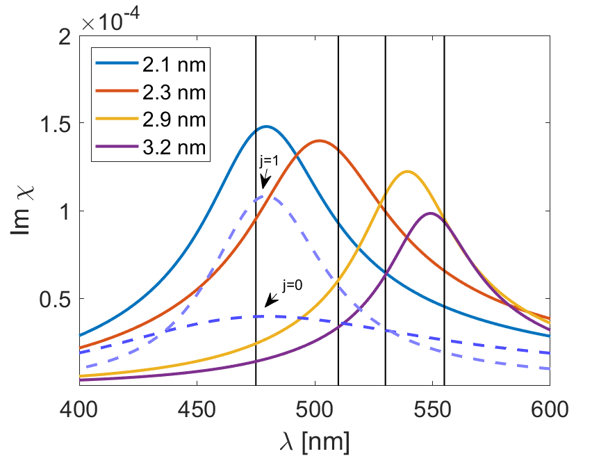
Figure 1: Absorption spectra of cylindrical quantum dots calculated for 4 values of the disk radius. Black lines mark the experimental data measured by Lee et al.Lee

We have calculated the absorption from the imaginary part of $\bar{\chi}_{QD}$ defined in Eq. (III), for a Cu₂O QD system and compare our theoretical predictions with the experimental results by Lee et al.Lee In the calculations the two lowest exciton states $j=0,1$ and the lowest confinement states in the $z$-direction were accounted for. The parameters used in calculation are summarized in Table 1. The results are shown on the Fig.1. Since the experiments in Ref.Lee were performed for spherical dots, we have slightly changed the dimensions, using an effective radius $R=4/5R_{spherical}$ and the disk height $L=1.6R$. One can see that the contributions from $j=0$ and $j=1$ states (dashed lines) overlap, forming single, wide absorption maximum. Our calculated theoretical curves agree very well with the experimental absorption curves from Ref.Lee We observe the increasing blue shift with decreasing QD radius, and the increasing oscillator strength with lowering the dimensions. As it was observedBorgohain ^-Zhou for the case of Cu₂O based QD, the excitonic transition energies depend strongly on the lateral extension.

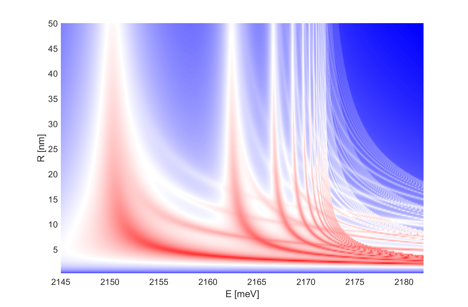
Figure 2: The absorption coefficient $\alpha$ of Cu₂O nanowire, calculated from (IV), as a function of the wire radius R.

The Fig. 2 shows the absorption coefficient (6) calculated for the case of a quantum wire, using the susceptibility given by Eq. (28). One can observe multiple excitonic states which diverge towards the higher energy as the wire radius approaches 0 and for small wire radius one may obtain a strong enhancement of the binding energies. The confinement states become more visible at low $R$. For sufficiently small radius, these lines mix and overlap, producing a complicated pattern. One can also observe that most of these confinement states are located above the gap energy; lower excitonic states are stronger bounded than the higher ones. These tendencies are in agreement with available experimental and theoretical results for Rydberg states of excitons in GaAs quantum wires okano ; banai .

As a next step, we consider a quantum well in the form of a plane-parallel slabs of Cu₂O. In our calculations, the dimensions in the $z$-direction varied from 20 nm to micrometer range, which corresponds to structures used in experiments by Takahata et al Takahata (lower limit) and by Kazimierczuk et al Kazimierczuk (upper limit). Such dimensions cover the regimes of QWs, WQWs, and exciton-polariton regime. For any regime the calculations were performed by methods appropriate to the given regime. The limits between these regimes are not sharply defined. For example, the thickness $L$=200 nm is large compared to the extension of the lowest exciton state (about 4 nm), but small compared to the extension of states with $j>10$. Therefore we used the criterion of the relation between the slab thickness and the wavelength of the wave propagating in the crystal, which equals to about 200 nm. We consider the slabs with $L<200$ nm as QWs and use the long-wave approximation, which, together with the assumption of infinite confinement potentials, leads to the expression (V) for the effective dielectric susceptibility and, in consequence, to the expression for the absorption coefficient. The absorption line shape resulting from Eq. (6) is shown in the lowest part of Fig. 3. We observe the overlapping of exciton and confinement states. For small $j$ and $N$ the exciton effect prevails, whereas for large values of $N$ the series of exciton resonances appears below every confinement state. These peaks exhibit a strong, roughly parabolic shift towards higher energy with decreasing $L$, which is similar to the case of quantum wire and typical for these structures in other semiconductors Christol . Eventually, the lines cross and mix together, creating a complicated spectrum, especially for $E>E_{g}$. Interestingly, due to the large number of confinement states present only in a thin crystal, the absorption coefficient is decreasing with $L$. However, the total absorption is still proportional to thickness, as shown in Fig. 4. One can also observe that the absorption discontinuity at the band gap is smeared out and disappears completely at for $L<200$ nm. The relative amplitude and shape of absorption peaks and the strong mixing of higher states are consistent with experimental observations by Khramtsov et al for the GaAs/GaAlAs quantum wells. Khramtsov For $L>200$ nm the long-wave approximation is not valid, and the methods of Sec. VI are used. The effect of confinement decreases, and the maxima related to the exciton states with $j=2,3...$ are visible. This effect is also observed in the central part of Fig. 3. When the considered crystal thickness is considerably larger that the wavelength inside the crystal, the reflection and transmission spectra will be strongly influenced by Fabry-Perot interference. One can observe that the absorption maxima on the Fig. 3 exhibit strong mixing for $L<200$ nm, which creates a very complicated transmission pattern.

Fig. 5 shows the exciton dispersion relation (VII), including polaritonic contribution which is represented by the term $(\mu/M_{tot})(ka^{*})^{2}$ in the denominator. Overall, the inclusion the polaritons gives a nonlinear shift to the position of the resonances; the higher states, which are closer to $E_{g}$ are more affected. It should be mentioned that such an effect could explain some discrepances observed in fitting a simple $j^{-2}$ model to the available experimental data; the Fig. 6 shows the comparison between absorption maxima positions measured by Kazimierczuk et al and our absorption spectrum calculated from (VII). For our fit, we have used the Rydberg energy $R=91.5$ meV and quantum defect $\delta=0.083$. With these values, we have obtained almost perfect fit to all excitonic peaks for $j=2\ldots 25$. Note that the quantum defect affects mostly low-energy states but cannot explain the apparent deviation from $j^{-2}$ relation for high states. This is easily visible in Fig. 7; even with proper fitting values, the standard relation, represented by straight line, cannot fit all the states. On the other hand, the nonlinear curve provided by polaritonic relation appears to be a much better fit.

The above indicated agreement can be understood as an indirect proof for existence of polariton waves. Another argument may come from experiment. Just at early stage of the research on Wannier-Mott excitons a number of experiments has been performed to manifest the existence of many transverse waves (polaritons) with fixed frequency and polarization, distinguished by the index of refraction (see Broser et al. Broser ). In particular, for a CdS crystal, Lebedev et al. Lebedev observed the simultaneous transmission of two polariton waves through a wedge shaped crystal and spatially separated them. As we have shown above, see Eq. (51), a similar situation occurs in a Cu₂O crystal: near any exciton resonance energy there are two polariton waves with wave vectors $k^{(j)}_{1,2}$, and different indices of refraction, propagating through the crystal. So we hope, that a similar experiment, as for the CdS crystal, can be performed for a Cu2O crystal, to give an unambiguous proof for the existence of polariton waves.

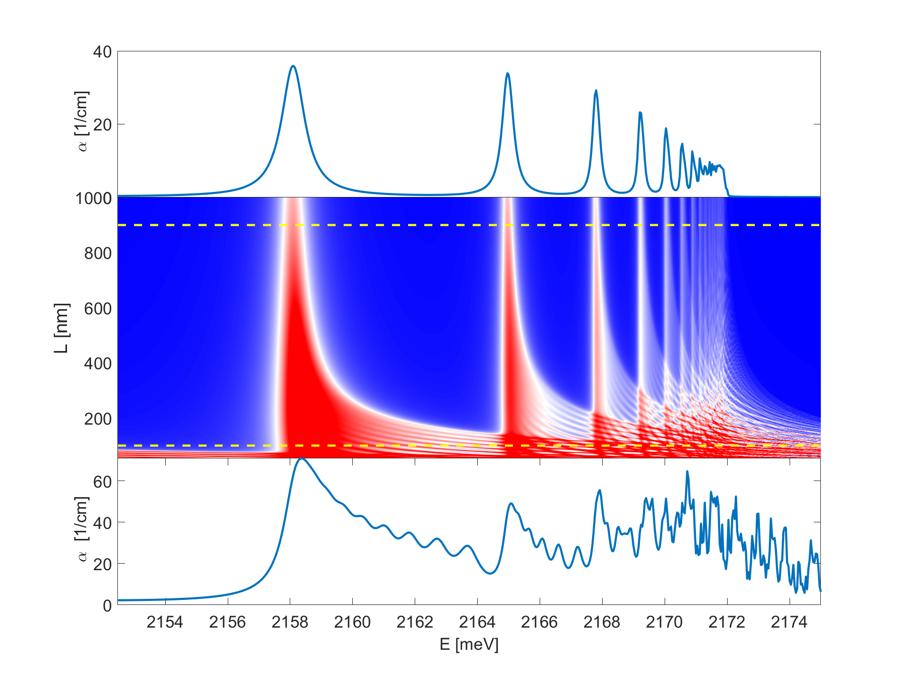
Figure 3: The absorption coefficient $\alpha$ of Cu₂O crystal, calculated from (V), as a function of crystal thickness. The top and bottom panels show cross-sections for thickness $L=900$ nm and $L=100$ nm, respectively.

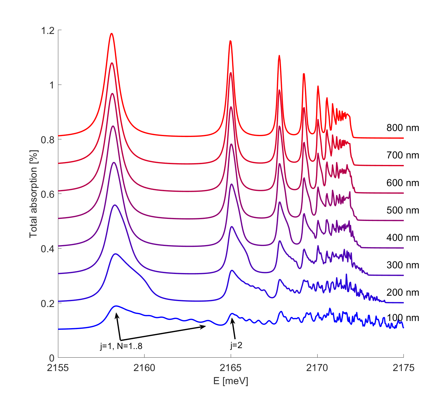
Figure 4: The absorption coefficient from Fig. (3), for selected values of thickness.

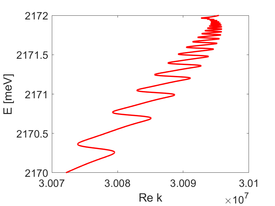
Figure 5: Polariton dispersion relation calculated from (VII).

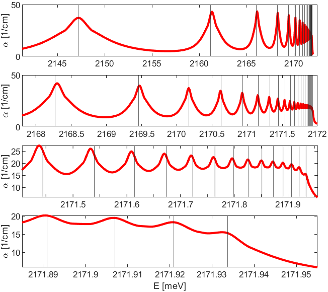
Figure 6: Excitonic absorption in Cu₂O crystal with polaritons calculated from (6) and (VII). Black lines are peaks from experimental data by Kazimierczuk et al.Kazimierczuk

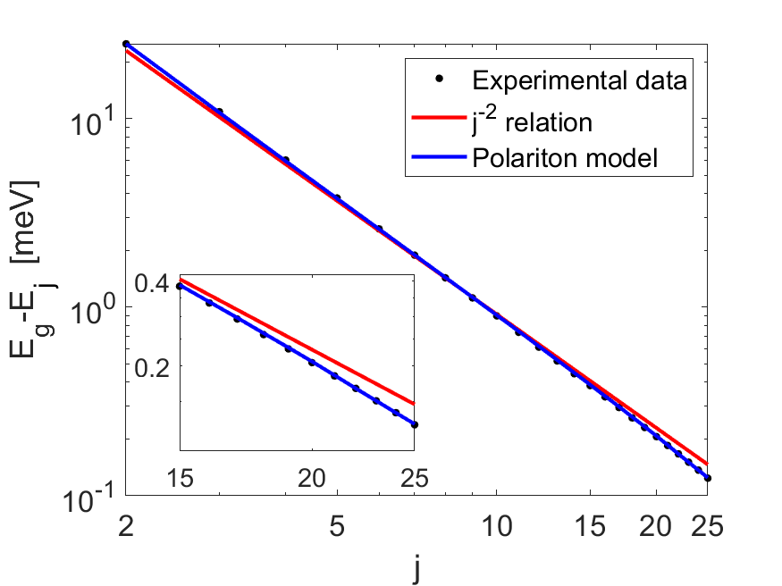
Figure 7: Absorption peaks position comparison between theory with (VII) or without polaritons to experimental data by Kazimierczuk et al.Kazimierczuk Line $j^{-2}$ added for reference.

Table 1: Band parameter values for Cu₂O, masses in free electron mass $m_{0}$, $R^{*}$ calculated from $(\mu/\epsilon_{b}^{2})\cdot 13600\,\hbox{meV}$,  $R^{*}_{e,h}=(m_{e,h}/\mu)R^{*},a^{*}_{e,h}=(\mu/m_{e,h})a^{*}$

Parameter	Value	Unit	Reference
$E_{g}$	2172.08	meV	Kazimierczuk
$R^{*}$	87.78	meV
$\Delta_{LT}$	$1.25\times 10^{-3}$	meV	Stolz
$m_{e}$	0.99	$m_{0}$	Naka
$m_{h}$	0.58	$m_{0}$	Naka
$\mu$	0.363	$m_{0}$
$M_{tot}$	1.56	$m_{0}$
$a^{*}$	1.1	nm	Kazimierczuk
$r_{0}$	0.22	nm	Zielinska.PRB
$\epsilon_{b}$	7.5		Kazimierczuk
${R_{e}^{*}}$	239.4	meV
${R^{*}_{h}}$	140.25	meV
${a^{*}_{e}}$	0.4	nm
${a^{*}_{h}}$	0.69	nm
$\Gamma_{j}$	3.88/$j^{3}$	meV	Kazimierczuk ; maser2

IX Conclusions

A theoretical solutions to model absorption spectra of low dimensional systems with Rydberg excitons in a wide range of system dimensions are presented. The optical absorption spectra of Cu₂O quantum dots of different sizes, quantum wires and quantum wells as well as for a bulk crystal are discussed. For each systems dimension the calculations were performed by methods appropriate to the considered regime leading to the analytical expression for the susceptibility. Results are compared with available experimental data, showing a good agreement and confirming that quantum confinement effects are evident from a blueshift in the optical absorption. In particular, the calculated spectra of all low-dimensional systems exhibit a smooth transition to the bulk absorption in the limit of large size of the nanostructure. For bulk crystals presented calculations performed in terms of microscopic boundary conditions for the exciton motion inside the crystal of finite size are in a good agreement with experimental spectra. Thus, we have shown that the existence of polaritons can explain the positions of exciton resonances with a higher accuracy than existing models.

References

- (1) T. Kazimierczuk, D. Fröhlich, S. Scheel, H. Stolz, and M. Bayer, Nature 514, 344 (2014).
- (2) J. Heckötter, M. Freitag, D. Fröhlich, M. Aßmann, M. Bayer, M. A. Semina, and M. M. Glazov, Phys. Rev. B 96, 125142 (2017).
- (3) M. Aßmann, J. Thewes, and M. Bayer, Nature Materials 15, 741 (2016).
- (4) J. Thewes, J. Heckötter, T. Kazimierczuk, M. Aßmann, D. Fröhlich, M. Bayer, M. A. Semina, and M. M. Glazov, Phys. Rev. Lett. 115, 027402 (2015).
- (5) F. Schöne, S.-O. Krüger, P.Grünwald, H. Stolz, M. Aßmann, J. Heckötter, J. Thewes, D. Fröhlich, and M. Bayer, Phys. Rev. B 93, 075203 (2016).
- (6) F. Schweiner, J. Main, and G. Wunner, Phys. Rev. B 95, 035202 (2017).
- (7) S. Zielinska-Raczyńska, D. A. Fishman, C. Faugeras, M. M. P. Potemski, P. H. M. van Loosdrecht, K. Karpiński, G. Czajkowski, and D. Ziemkiewicz, New J. Phys. 21, 103012 (2019).
- (8) S. Zielinska-Raczyńska, D. Ziemkiewicz, and G. Czajkowski, Phys. Rev. B 97, 165205 (2018).
- (9) V. Walther, R. Johne, and T. Pohl, Nature Communications 9, 1309 (2018).
- (10) S. Zielińska-Raczyńnska, G. Czajkowski, K. Karpiński, and D. Ziemkiewicz, Phys. Rev. B 99, 245206 (2019).
- (11) F. Schweiner, J. Ertl, J. Main, G. Wunner, and Ch. Uihlein, Phys. Rev. B 96, 245202 (2017).
- (12) J. Heckötter, M. Freitag, D. Fröhlich, M. Aßmann, M. Bayer, P. Grünwald, F. Schöne, D. Semkat, H. Stolz, and S. Scheel, Phys. Rev. Lett. 121, 097401 (2018).
- (13) S. Zielińska-Raczyńska, G. Czajkowski, and D. Ziemkiewicz, Phys. Rev. B 93, 075206 (2016).
- (14) S. Zielińska-Raczyńska, D. Ziemkiewicz, and G. Czajkowski, Phys. Rev. B 94, 045205 (2016).
- (15) S. Zielińska-Raczyńska, D. Ziemkiewicz, and G. Czajkowski, Phys. Rev. B 95, 075204 (2017).
- (16) D. Ziemkiewicz, S. Zielińska - Raczyńska, Optics Express 27, 12, 16983-16994 (2019).
- (17) S. Zielinska-Raczyńska, D. Ziemkiewicz, , G. Czajkowski, and K. Karpiński, Phys. Status Solidi B 256, 1800502 (2019).
- (18) N. Naka, I. Akimoto, M. Shirai, and Ken-ichi Kan’no, Phys. Rev. B 85, 035209 (2012).
- (19) M. Takahata, K. Tanaka, and N. Naka, Phys. Rev. B 97, 205305 (2018).
- (20) A. Konzelmann, B. Frank, and H. Giessen, Phys. B: At. Mol. Opt. Phys. 53, 024001 (2020).
- (21) S. Zielińska-Raczyńska, D. Ziemkiewicz, and G. Czajkowski, Phys. Rev. B 93, 075206 (2016).
- (22) A. Stahl, I. Balslev, Electrodynamics of the semiconductor band edge, Springer, 1987.
- (23) J. Heckötter, D. Frölich, M. Aßmann, and M. Bayer, Physics of the Solid State 60, 1595 (2018).
- (24) Handbook of Self-Assembled Semiconductor Nanostructures for Novel Devices in Photonics and Electronics, Ed. by M. Henini (Elsevier, Amsterdam, 2008).
- (25) D. S. Chuu, C. M. Hsiao, and W. N. Mei, Phys Rev. B, 46, 3898 (1992).
- (26) M. Abramowitz and I. Stegun, Handbook of Mathematical Functions (Dover Publications, New York, 1965).
- (27) T. F. Gallagher, Rep. Prog. Phys. 51, 143 (1988).
- (28) F. Schöne,S. Krüger, P. Grünwald, M. Assmann, J. Heckötter, J. Thewes, H. Stolz, D. Fröhlich, M. Bayer, and S. Scheel, J. Phys. B: At. Mol. Opt. Phys. 49 134003 (2016).
- (29) H. Stolz, F. Schöne, and D. Semkat, N. Journ. Phys. 20, 023019 (2018).
- (30) T. Kitamura, M. Takahata, and N. Naka, J. Luminescence 192, 808 (2017).
- (31) G. Czajkowski, F. Bassani, and L. Silvestri, Rivista del Nuovo Cimento 26, 1-150 (2003).
- (32) N. F. Mott and H. S. W. Masey, The theory of atomic collisions (Clarendon Press, Oxford, 1965).
- (33) Scully, M.; Zubairy, M. Quantum Optics. Cambridge University Press: Cambridge, UK, 1997.
- (34) H. C. Schneider, F. Jahnke, S. W. Koch, J. Tignon, T. Hasche, and D. S. Chemla, Phys. Rev. B 63, 045202 (2001).
- (35) S. I. Pekar, Crystal Optics and Additional Light Waves (Benjamin-Cummings, Menlo Park, 1983).
- (36) J. J. Hopfield and D. G. Thomas, Phys. Rev. 132, 563 (1963).
- (37) A. D’Andrea and R. Del Sole, Phys. Rev. B 41, 1413 (1990).
- (38) J. L. Birman, Electrodynamics and Nonlocal Optical Effects mediated by Excitonic Polaritons, in Excitons, Modern Problems in Condensed Matter Sciences, edited by E. I. Rashba and M. G. Sturge, Vol.2 (North-Holland, Amsterdam, 1982), p. 27.
- (39) V. M. Agranovich and V. L. Ginzburg, Crystal optics with spatial dispersion and excitons (Springer Verlag, Berlin, 1984).
- (40) A. D’Andrea and R. Del Sole, Phys. Rev. B 32, 2337 (1985).
- (41) K. Cho, J. Phys. Soc. Japan 55, 4113 (1986).
- (42) G. Czajkowski, F. Bassani, and A. Tredicucci, Phys. Rev. B 54, 2035 (1996).
- (43) V. M. Agranovich, Excitations in Organic Solids (Oxford University Press, Oxford, 2009).
- (44) H. Kalt and C. F. Klingshirn, Semiconductor optics 1. Linear optical properties of semiconductors, Vth ed. (Springer, Berlin, 2019).
- (45) D. Schiumarini, N. Tomassini, L. Pilozzi, and A. D’Andrea, Phys. Rev. B 82, 075303 (2010).
- (46) M. Y. Lee, S-H. Kim, and I-K. Park, Physica B, 500, 4, (2016).
- (47) K. Borgohain, N. Murase, and S. Mahamuni, J. Applied Phys. 92, 1292 (2002).
- (48) Y. Zhou, Y. Wang, and Y. Guo, Materials Letters, 254, 336 (2019).
- (49) M. Okano, Y. Kanemitsu, S. Chen, T. Mochizuki, M. Yoshita, H. Akiyama, L. N. Pfeiffer, and K. W. West, Phys. Rev. B 86, 085312 (2012).
- (50) L. Bányai, I. Galbraith, C. Ell, and H. Haug, Phys. Rev. B 36, 6099 (1987).
- (51) P. Christol, P. Lefebvre, and H. Mathieu, J. Appl. Phys. 74(9), 5626 (1993).
- (52) E. S. Khramtsov, P. S. Grigoryev, D. K. Loginov, I. V. Ignatiev, Yu. P. Efimov, S. A. Eliseev, P. Yu. Shapochkin, E. L. Ivchenko, and M. Bayer, Phys Rev. B 99, 035431 (2019).
- (53) I. Broser, R. Broser, E. Beckmann, and E. Birkicht, Solid State Commun. 39, 1209 (1981), https://doi.org/10.1016/0038-1098(81)91115-7.
- (54) M. V. Lebedev, M. I. Strashnikova, V. B. Timofeev, and V. V. Chernyi, JETP Lett. 39, 440 (1984).