A robust method based on LOVO functions for solving least squares problems

Abstract

The robust adjustment of nonlinear models to data is considered in this paper. When data comes from real experiments, it is possible that measurement errors cause the appearance of discrepant values, which should be ignored when adjusting models to them. This work presents a Lower Order-value Optimization (LOVO) version of the Levenberg-Marquardt algorithm, which is well suited to deal with outliers in fitting problems. A general algorithm is presented and convergence to stationary points is demonstrated. Numerical results show that the algorithm is successfully able to detect and ignore outliers without too many specific parameters. Parallel and distributed executions of the algorithm are also possible, allowing for the use of larger datasets. Comparison against publicly available robust algorithms shows that the present approach is able to find better adjustments in well known statistical models.

Keywords: Lower Order-Value Optimization, Levenberg-Marquardt, Outlier Detection, Robust Least Squares

1 Introduction

In this work we are interested in studying the following problem: given a dataset $\mathcal{R}=\{(t_{i},y_{i}),i=1,...,r\}$ of points in $\mathbb{R}^{m}\times\mathbb{R}$, resulting from some experiment, we want to find a model $\varphi:\mathbb{R}^{m}\rightarrow\mathbb{R}$ for fitting this dataset free from influence of possible outliers. In a more precise way, given a model $\varphi(t)$ depending on $n$ parameters ($x\in\mathbb{R}^{n}$), that is, $\varphi(t)=\phi(x,t)$, we want to find a set $\mathcal{P}\subset\mathcal{R}$ with $p$ elements and parameters $\overline{x}\in\mathbb{R}^{n}$, such that $\phi(\overline{x},t_{i})\approx y_{i}$, $\forall(t_{i},y_{i})\in\mathcal{P}$ (in the least squares sense). The $r-p$ remaining elements in $\mathcal{R}-\mathcal{P}$ are the possible outliers.

There are several definitions of what an outlier is. The definition that best suits the present work concerns to errors in $y_{i}$, that is, grotesque errors in evaluation of some measure for a given and reasonably precise $t_{i}$. This is somewhat different from the geometric interpretation of outliers, in the sense that the point $(t_{i},y_{i})$ is (geometrically) very far from the graph of a function that one wants to find. Typically in our tests, outliers are present when there are errors resulting from the measurement of some experiment. As a consequence, their presence may contaminate the obtained model and, therefore, deteriorate or limit its use. There are several strategies to handle the presence of outliers in datasets [7, 10, 20, 21]. In a more recent approach, as highlighted by [11] and references therein, techniques based on machine learning are exploited in the context of deal with a large amount of data, lack of models and categorical variables.

In order to get a fitting model free from influence of outliers, we use an approach based on Low Order-Value Optimization (LOVO) [3] which is defined as follows. Consider $R_{i}:\mathbb{R}^{n}\rightarrow\mathbb{R}$, $i=1,...,r$. Given $x\in\mathbb{R}^{n}$, we can sort $\{R_{i}(x),i=1,...,r\}$ in ascending order:

$$R_{i_{1}(x)}(x)\leq R_{i_{2}(x)}(x)\leq...\leq R_{i_{k}(x)}(x)\leq\dots\leq R_{i_{r}(x)}(x),$$ (1)

where $i_{k}(x)$ is the $i_{k}$-th smallest element in that set, for the given value of $x$. Given $0<p\leq r$, the LOVO function is defined by

$$S_{p}(x)=\sum_{k=1}^{p}R_{i_{k}(x)}(x)$$ (2)

and the LOVO problem is

$$\min S_{p}(x).$$ (3)

Essentially, this problem can be seen as a generalization of nonlinear least squares, as elucidated in [3]. To reiterate this affirmation, we can consider $\varphi(t)=\phi(x,t)$ as the model selected for fitting,and define $R_{i}(x)=\dfrac{1}{2}(F_{i}(x))^{2}$, where $F_{i}(x)=y_{i}-\phi(x,t_{i}),i=1,...,r$. Thus, we have the particular LOVO problem

$$\min S_{p}(x)=\min\sum_{k=1}^{p}R_{i_{k}(x)}(x)=\min\sum_{k=1}^{p}\frac{1}{2}(F_{i_{k}(x)}(x))^{2}.$$ (4)

Each $R_{i}$ is a residual function. Consequently, if we assume $p=r$ the LOVO problem is the classical least squares problem. When $p<r$ the parameter $\bar{x}\in\mathbb{R}^{n}$ that solves (4) defines a model $\phi(\bar{x},t)$ free from the influence of the worst $r-p$ deviations. Throughout this work, $p$ is also know as the number of trusted points.

Several applications can be modeled in the LOVO context, as is illustrated in [16, 3, 2, 5, 14]. An excellent survey about LOVO problems and variations is given in [15]. Although it is well known that LOVO deals with detection of outliers, there is a limitation: the mandatory definition of the value $p$, which is associated to the number of possible outliers. This is the main gap that this paper intends to fill. We present a new method that combines a voting schema and an adaptation of the Levenberg-Marquardt algorithm in context of LOVO problems.

Levenberg-Marquardt algorithms can be viewed as a particular case of trust-region algorithms, using specific models to solve nonlinear equations. In [2], a LOVO trust-region algorithm is presented with global and local convergence properties and an application to protein alignment problems. Second-order derivatives were needed in the algorithm for the local convergence analysis. In least-squares problems, as the objective function has a well known structure, Levenberg-Marquardt algorithms use a linear model for the adjustment function, instead of a quadratic model for the general nonlinear function. This approach eliminates the necessity of using second-order information for the model. More details of Levenberg-Marquardt methods can be found in [19].

In [22], outlier detection techniques are classified in 7 groups for problems of data streaming: Statistic-based, depth-based, deviation-based, distance-based, clustering-based, sliding-window-based and autoregression-based. In [24], classification is divided only between geometric and algebraic algorithms for robust curve and surface fitting. The approach used in this work is clearly algebraic, strongly based in the fact that the user knows what kind of model is to be used. Although models are used, we make no assumption on the distribution of the points, so we do not fit clearly in any of the types described in [22]. We also make the assumption that the values $t_{i}$ are given exactly, what is called as fixed-regressor model in [19].

This work deals with the robust adjustment of models to data. A new version of the Levenberg-Marquardt algorithm for LOVO problems is developed, so the necessity of second-order information is avoided. In addition, the number of possible outliers is estimated by a voting schema. The main difference of the proposed voting schema is that it is based in the values of $p$ which has, by definition, a discrete domain. In other techniques, such as the Hough Transform [12, 8, 13, 23], continuous intervals of the model’s parameters are discretized. Also, the increase in the number of parameters to adjust does not impact the proposed voting system. The main improvements of this work can be stated as follows

• a Levenberg-Marquardt algorithm with global convergence for LOVO problems is developed, which avoids the use of second-order information such as in [2];

• a voting schema based on the values of $p$ is developed, whose size does not increase with the size or discretization of the parameters of the model;

• extensive numerical results are presented, which show the behavior of the proposed method and are also freely available for download.

This work is organized as follows. In Section 2 we describe the Levenberg-Marquardt algorithm in the LOVO context and demonstrate its convergence properties. In Section 3 the voting schema is discussed, which will make the LOVO algorithm independent of the choice of $p$ and will be the basis of the robust fitting. Section 4 is devoted to the discussion of the implementation details and comparison against other algorithms for robust fitting. Finally, in Section 5 we draw some conclusions of the presented strategy.

2 The Levenberg-Marquardt method for LOVO problems

Following [3], let us start this section by pointing out an alternative definition of LOVO problems for theoretical purposes. Denoting $\mathcal{C}=\{\mathcal{C}_{1},...,\mathcal{C}_{q}\}$ the set of all combinations of the elements $\{1,2,...,r\}$ taken $p$ at a time, we can define for each $i\in\{1,...,q\}$ the following functions

$$f_{i}(x)=\sum_{k\in\mathcal{C}_{i}}R_{k}(x)$$ (5)

and

$$f_{min}(x)=\min\{f_{i}(x),i=1,...,q\}.$$ (6)

It is simple to note that $S_{p}(x)=f_{min}(x)$ which is a useful notation in our context. Moreover, it is possible to note that $S_{p}$ is a continuous function if $f_{i}$ is a continuous function for all $i=1,...,q$, but, even assuming differentiability over $f_{i}$, we cannot guarantee the same for $S_{p}$. In addition, since $R_{k}(x)=\dfrac{1}{2}(F_{k}(x))^{2},k\in\mathcal{C}_{i},i=1,...,q$ we can write

$$f_{i}(x)=\frac{1}{2}\sum_{k\in\mathcal{C}_{i}}F_{k}(x)^{2}=\dfrac{1}{2}\|F_{\mathcal{C}_{i}}(x)\|^{2}_{2}.$$ (7)

Throughout this work, following (7), given a set $\mathcal{C}_{i}\in\mathcal{C}$, $F_{\mathcal{C}_{i}}(x):\mathbb{R}^{n}\to\mathbb{R}^{p}$ will always refer to the map that takes $x$ to the $p$-sized vector composed by the functions $F_{k}(x)$ defined by (4), for $k\in\mathcal{C}_{i}$ in any fixed order. Similarly, $J_{\mathcal{C}_{i}}(x)$ is defined as the Jacobian of this map. Additionally, we assume the continuous differentiability for $F_{i}$, $i=1,...,r$.

The goal of this section is to define a version of Levenberg-Marquardt method (LM) to solve the specific problem (4), for a given $p$, as well as a result on global convergence. The new version will be called by simplicity LM-LOVO. It is well known that the Levenberg-Marquardt method proposed in [17] is closely related to trust-region methods and our approach is based on it. Consequently, some definitions and remarks are necessary.

Definition 2.1.

Given $x\in\mathbb{R}^{n}$ we define the minimal function set of $f_{min}$ in $x$ by

$$I_{min}(x)=\{i\in\{1,\dots,q\}\ |\ f_{min}(x)=f_{i}(x)\}.$$

In order to define a search direction for LM-LOVO at the current point $x_{k}$, we choose an index $i\in I_{min}(x_{k})$ and compute the direction defined by the classical Levenberg-Marquardt method using $f_{i}(x)$, that is, the search direction $d_{k}\in\mathbb{R}^{n}$ is defined as the solution of

$$\min_{d\in\mathbb{R}^{n}}m_{k,i}(d)=\dfrac{1}{2}\|F_{\mathcal{C}_{i}}+J_{\mathcal{C}_{i}}(x_{k})d\|_{2}^{2}+\dfrac{\gamma_{k}}{2}\|d\|_{2}^{2},$$

where $\gamma_{k}\in\mathbb{R}^{+}$ is the damping parameter. Equivalently, the direction $d$ can be obtained by

$$(J_{\mathcal{C}_{i}}(x_{k})^{T}J_{\mathcal{C}_{i}}(x_{k})+\gamma_{k}I)d=-\nabla f_{i}(x_{k}),$$ (8)

where $\nabla f_{i}(x_{k})=J_{\mathcal{C}_{i}}(x_{k})^{T}F_{\mathcal{C}_{i}}(x_{k})$ and $I\in\mathbb{R}^{n\times n}$ is the identity matrix.

To ensure sufficient decrease in the defined search direction, we can consider a similar strategy of trust-region methods, which involves monitoring the actual decrease (given by $f_{min}$) and the predicted decrease (given by $m_{k,i}$) at direction $d_{k}$:

$$\rho_{k,i}=\dfrac{f_{min}(x_{k})-f_{min}(x_{k}+d_{k})}{m_{k,i}(0)-m_{k,i}(d_{k})}.$$ (9)

We observe that, since $i\in I_{min}(x_{k})$, $m_{k,i}$ is also a local model for $f_{min}$ at $x_{k}$. In practice, $f_{min}$ can safely be replaced by $f_{i}$ in (9). We formalize the conceptual algorithm LM-LOVO in the Algorithm 1.

Input: $x_{0}\in\mathbb{R}^{n}$, $\lambda_{min},\epsilon,\lambda_{0}\in\mathbb{R}_{+}$, $\overline{\lambda}>1,\mu\in(0,1)$ and $p\in\mathbb{N}$

Output: $x_{k}$

Set $k\leftarrow 0$;

1Select $i_{k}\in I_{min}(x_{k})$;

$\lambda\leftarrow\lambda_{k}$;

2if $\|\nabla f_{i_{k}}(x_{k})\|_{2}<\epsilon$ then

       Stop the algorithm, $x_{k}$ is an approximate solution for the LOVO problem;

      

3$\gamma_{k}\leftarrow\lambda\|\nabla f_{i_{k}}(x_{k})\|^{2}_{2}$;

Compute $d_{k}$ the solution of the linear system (8);

Calculate $\rho_{k,i_{k}}$ as described in (9);

4if $\rho_{k,i_{k}}<\mu$ then

       $\lambda\leftarrow\overline{\lambda}\lambda$;

       Go back to the Step 1;

      

else

       Go to the Step 1;

      

5$\lambda_{k+1}\in[\max\{\lambda_{min},\lambda/\overline{\lambda}\},\lambda]$;

$x_{k+1}\leftarrow x_{k}+d_{k}$;

$k\leftarrow k+1$ and go back to the Step 1 ;

Algorithm 1 LM-LOVO – Levenberg-Marquardt for the LOVO problem.

In what follows, we show that Algorithm 1 is well defined and converges to stationary points of the LOVO problem. We begin with some basic assumptions on the boundedness of the points generated by the algorithm and on the smoothness of the involved functions.

Assumption 2.2.

The level set

$$C(x_{0})=\{x\in\mathbb{R}^{n}\ |\ f_{min}(x)\leq f_{min}(x_{0})\}$$

is a bounded set of $\mathbb{R}^{n}$ and the functions $f_{i}$, $i=1,\dots,r$, have Lipschitz continuous gradients with Lipschitz constants $L_{i}>0$ in an open set containing $C(x_{0})$.

The next proposition is classical in the literature of trust-region methods and ensures decrease of $m_{k,{i_{k}}}(.)$ on the Cauchy direction. It was adapted to the LOVO context.

Proposition 2.3.

Given $x_{k}\in\mathbb{R}^{n}$, $\gamma\in\mathbb{R}_{+}$ and ${i_{k}}\in\{1,\dots,r\}$, the descent direction obtained from

$$\widehat{t}=argmin_{t\in\mathbb{R}}\ \ \{m_{k,i_{k}}(-t\nabla f_{i_{k}}(x_{k})\}$$

and expressed by $d^{C}(x_{k})=-\widehat{t}\nabla f_{i_{k}}(x_{k})\in\mathbb{R}^{n}$, satisfies

$$m_{k,i_{k}}(0)-m_{k,i_{k}}(d^{C}(x_{k}))\geq\dfrac{\theta\|\nabla f_{i_{k}}(x_{k})\|^{2}_{2}}{2(\|J_{\mathcal{C}_{i}}(x_{k})\|^{2}_{2}+\gamma)}.$$ (10)

Proof.

The proof follows from [4, Section 3]. ∎

Since the Cauchy’s step is obtained by the constant that minimizes the model $m_{k,i_{k}}(.)$ on the direction of the gradient vector, we can conclude that

$$m_{k,i_{k}}(0)-m_{k,i_{k}}(d_{k})\geq\dfrac{\theta\|\nabla f_{i_{k}}(x)\|^{2}_{2}}{2(\|J_{\mathcal{C}_{i}}({x_{k}})\|^{2}_{2}+\gamma)},$$ (11)

since $d_{k}\in\mathbb{R}^{n}$ from (8) is the global minimizer of $m_{k,i_{k}}$.

Inspired by [4], we present Lemma 2.4 that shows that Step 1 is always executed by Algorithm 1 if $\lambda$ is chosen big enough.

Lemma 2.4.

Let $x_{k}\in\mathbb{R}^{n}$ and $i_{k}\in I_{min}(x_{k})$ be a vector and an index fixed in the Step 1 of the Algorithm 1. Then, the Step 1 of the Algorithm 1 will be executed a finite number of times.

Proof.

To achieve this goal, we will show that

$$\lim_{\lambda\rightarrow\infty}\rho_{k,i_{k}}=2.$$

For each $\lambda$ fixed in the Step 1 of the Algorithm 1, we have that

$$\left|1-\dfrac{\rho_{k,i_{k}}}{2}\right| = \left|1-\dfrac{f_{min}(x_{k})-f_{min}(x_{k}+d_{k})}{2(m_{k,i_{k}}(0)-m_{k,i_{k}}(d_{k})}\right|$$

$$= \left|\dfrac{2m_{k,i_{k}}(0)-2m_{k,i_{k}}(d_{k})-f_{min}(x_{k})+f_{min}(x_{k}+d_{k})}{2(m_{k,i_{k}}(0)-m_{k,i_{k}}(d_{k}))}\right|$$

$$= \left|\dfrac{f_{min}(x_{k}+d_{k})+f_{min}(x_{k})-2m_{k,i_{k}}(d_{k})}{2(m_{k,i_{k}}(0)-m_{k,i_{k}}(d_{k}))}\right|$$

From Taylor series expansion and the Lipschitz continuity of $\nabla f_{i_{k}}(x_{k})$

$$f_{i_{k}}(x_{k}+d_{k})\leq f_{i_{k}}(x_{k})+\nabla f_{i_{k}}(x_{k})^{T}d_{k}+\dfrac{L_{i_{k}}}{2}\|d_{k}\|^{2}_{2}.$$ (13)

By equation (13) and the definition of $f_{min}$, we obtain

$$f_{min}(x_{k}+d_{k})\leq f_{i_{k}}(x_{k}+d_{k})\stackrel{{\scriptstyle\tiny{\eqref{eq:2prof-lem2}}}}{{\leq}}f_{i_{k}}(x_{k})+\nabla f_{i_{k}}(x_{k})^{T}d_{k}+\dfrac{L_{i_{k}}}{2}\|d_{k}\|^{2}_{2}.$$ (14)

Using (14) and the definition of $m_{k,i_{k}}$ in  (2), we get

$$\begin{split}\left|1-\right.&\left.\dfrac{\rho_{k,i_{k}}}{2}\right|=\left|\dfrac{f_{min}(x_{k}+d_{k})+f_{min}(x_{k})-2m_{k,i_{k}}(d_{k})}{2(m_{k,i_{k}}(0)-m_{k,i_{k}}(d_{k}))}\right|\\ &=\left|\dfrac{f_{min}(x_{k}+d_{k})+f_{i_{k}}(x_{k})}{2(m_{k,i_{k}}(0)-m_{k,i_{k}}(d_{k}))}\right.-\left.\dfrac{\|F_{\mathcal{C}_{i}}(x_{k})+J_{\mathcal{C}_{i}}(x_{k})d_{k}\|^{2}_{2}+\gamma_{k}\|d_{k}\|^{2}_{2}}{2(m_{k,i_{k}}(0)-m_{k,i_{k}}(d_{k}))}\right|\\ &=\left|\dfrac{f_{min}(x_{k}+d_{k})-f_{i_{k}}(x_{k})-2\nabla f_{i_{k}}(x_{k})^{T}d_{k}}{2(m_{k,i_{k}}(0)-m_{k,i_{k}}(d_{k}))}\right.\\ &\qquad\left.-\dfrac{d_{k}^{T}\left(J_{\mathcal{C}_{i}}(x_{k})^{T}J_{\mathcal{C}_{i}}(x_{k})+\gamma_{k}I\right)d_{k}}{2(m_{k,i_{k}}(0)-m_{k,i_{k}}(d_{k}))}\right|\\ &\stackrel{{\scriptstyle\tiny{\eqref{eq:alt_direc}}}}{{=}}\left|\dfrac{f_{min}(x_{k}+d_{k})-f_{i_{k}}(x_{k})-\nabla f_{i_{k}}(x_{k})^{T}d_{k}}{2(m_{k,i_{k}}(0)-m_{k,i_{k}}(d_{k}))}\right|\\ &\stackrel{{\scriptstyle\tiny{\eqref{eq:3prof-lem2}}}}{{\leq}}\left|\dfrac{L_{i_{k}}\|d_{k}\|^{2}_{2}}{4(m_{k,i_{k}}(0)-m_{k,i_{k}}(d_{k}))}\right|\end{split}$$ (15)

From (8) and the definition of $\gamma_{k}$, we note that

$$\|d_{k}\|_{2}\leq\dfrac{\|\nabla f_{i_{k}}(x_{k})\|_{2}}{\sigma_{k}+\gamma_{k}}\leq\dfrac{\|\nabla f_{i_{k}}(x_{k})\|_{2}}{\gamma_{k}}=\dfrac{1}{\|\nabla f_{i_{k}}(x_{k})\|_{2}\lambda},$$ (16)

where $\sigma_{k}=\sigma_{min}(J_{\mathcal{C}_{i}}(x_{k})^{T}J_{\mathcal{C}_{i}}(x_{k}))$ and $\sigma_{min}(B)$ represents the smallest eigenvalue of $B$.

Replacing (16) in (15), we obtain

$$\begin{split}\left|1-\dfrac{\rho_{k,i_{k}}}{2}\right|&\leq\left|\dfrac{\dfrac{L_{i_{k}}}{\|\nabla f_{i_{k}}(x_{k})\|^{2}_{2}\lambda^{2}}}{4(m_{k,i_{k}}(0)-m_{k,i_{k}}(d_{k}))}\right|\stackrel{{\scriptstyle\eqref{eq:dec-cauchy}}}{{\leq}}\left|\dfrac{\dfrac{L_{i_{k}}}{\|\nabla f_{i_{k}}(x_{k})\|^{2}_{2}\lambda^{2}}}{\dfrac{4\theta\|\nabla f_{i_{k}}(x_{k})\|^{2}_{2}}{2(\|J_{\mathcal{C}_{i}}(x_{k})\|^{2}_{2}+\gamma_{k})}}\right|\\ &=\dfrac{(\|J_{\mathcal{C}_{i}}(x_{k})\|^{2}_{2}+\gamma_{k})L_{i_{k}}}{2\theta\|\nabla f_{i_{k}}(x_{k})\|^{4}_{2}\lambda^{2}}\leq\left(\dfrac{\|J_{\mathcal{C}_{i}}(x_{k})\|^{2}_{2}}{\epsilon^{4}}+\dfrac{1}{\epsilon^{2}}\right)\dfrac{L_{i_{k}}}{2\theta\lambda},\end{split}$$ (17)

where the last inequality comes from the definition of $\gamma_{k}$ in Algorithm 1 and assuming that $\lambda\geq 1$, which can always be enforced.

Using (17), since the Jacobian $J_{\mathcal{C}_{i}}$ is bounded in $C(x_{0})$, we conclude that

$$\lim_{\lambda\rightarrow\infty}\left|1-\dfrac{\rho_{k,i_{k}}}{2}\right|=0,$$

which proves the result. ∎

Our studies move toward showing convergence results for Algorithm 1 to stationary points. At this point we should be aware of the fact that LOVO problems admit two types of stationary condition: weak and strong [2].

Definition 2.5.

A point $x^{*}$ is a weakly critical point of (3) when $x^{*}$ is a stationary point of $f_{i}$ for some $i\in I_{min}(x^{*})$. A point $x^{*}$ is a strongly critical point of (3) if $x^{*}$ is a stationary point of $f_{i}$ for all $i\in I_{min}(x^{*})$.

Although the strongly critical condition is theoretically interesting, in this work we are limited to the proof of weakly critical, since this second type is less expensive to verify in practice and therefore more common to deal with. The global convergence to weakly critical points is given by Theorem 2.6.

Theorem 2.6.

Let $\{x_{k}\}_{k\in\mathbb{N}}$ be a sequence generated by Algorithm 1. Consider $\mathcal{K}^{\prime}=\{k\ |\ i_{k}=i\}\subset\mathbb{N}$ an infinite subset of indexes for $i\in\{1,\dots,r\}$ and assume that Assumption 2.2 holds. Then, for all $x_{0}\in\mathbb{R}^{n}$, we have

$$\lim_{k\in\mathcal{K}^{\prime}}\|\nabla f_{i}(x_{k})\|_{2}=0.$$

Proof.

Clearly, there is an index $i$ chosen an infinite number of times by Algorithm 1 since $\{1,\dots,r\}$ is a finite set.

Let us suppose by contradiction that, for this index $i$, there exist $\epsilon>0$ and $K\in\mathbb{N}$ such that $\|\nabla f_{i}(x_{k})\|_{2}\geq\epsilon$, for all $k\geq K$.

Therefore, for each $k\geq K$, we obtain by the Step 1 of Algorithm 1 that $\lambda_{k}\leq\lambda_{K}$. Additionally, we get

$$\dfrac{f_{min}(x_{k})-f_{min}(x_{k}+d_{k})}{m_{k,i}(0)-m_{k,i}(d_{k})}\geq\mu$$

$$\Leftrightarrow f_{min}(x_{k})-f_{min}(x_{k+1})\geq\mu(m_{k,i}(0)-m_{k,i}(d_{k}))$$

$$\Leftrightarrow f_{min}(x_{k})-f_{min}(x_{k}+d_{k})\stackrel{{\scriptstyle\eqref{eq:dec-cauchy}}}{{\geq}}\mu\left(\theta\dfrac{\|\nabla f_{i}(x_{k})\|_{2}^{2}}{\|J_{\mathcal{C}_{i}}(x_{k})\|^{2}_{2}+\gamma_{k}}\right)$$

$$\Leftrightarrow f_{min}(x_{k})-f_{min}(x_{k}+d_{k})\geq\left(\dfrac{\mu\theta\epsilon^{2}}{\|J_{\mathcal{C}_{i}}(x_{k})\|^{2}_{2}+\epsilon^{2}\lambda_{k}}\right)$$

$$\Leftrightarrow f_{min}(x_{k})-f_{min}(x_{k}+d_{k})\geq\left(\dfrac{\mu\theta\epsilon^{2}}{\max_{k\geq K}\{\|J_{\mathcal{C}_{i}}(x_{k})\|^{2}_{2}\}+\epsilon^{2}\lambda_{K}}\right)$$

$$\Leftrightarrow f_{min}(x_{k}+d_{k})-f_{min}(x_{k})\leq-\left(\dfrac{\mu\theta\epsilon^{2}}{c}\right),$$ (18)

where $c=\max_{k\geq K}\{\|J_{\mathcal{C}_{i}}(x_{k})\|^{2}_{2}\}+\epsilon^{2}\lambda_{K}$.

Since $f_{min}$ is bounded from below and decreases by the constant value $\mu\theta\epsilon^{2}/c$ at every iteration $k\geq K$, we have, using the continuity of $f_{min}$, that the sequence $f_{min}(x_{k}+d_{k})$ converges to the minimizer of

$$\min_{x\in\mathbb{R}^{n}}\quad f_{min}(x)$$

and, therefore,

$$\lim_{k\in\mathcal{K}^{\prime}}f_{min}(x_{k}+d_{k})-f_{min}(x_{k})=0.$$ (19)

Using (18) and (19) we have that

$$\lim_{k\in\mathcal{K}^{\prime}}\dfrac{\mu\theta\epsilon^{2}}{\max_{k\geq K}\{\|J_{\mathcal{C}_{i}}(x_{k})\|_{2}\}+\epsilon^{2}\lambda_{k}}=0.$$

Consequently $\lim_{k\in\mathcal{K}^{\prime}}\lambda_{k}=\infty$, which contradicts inequality $\lambda_{k}\leq\lambda_{K}<\infty$. We conclude that there is no such $\epsilon$ and, therefore,

$$\lim_{k\in\mathcal{K}^{\prime}}\|\nabla f_{i}(x_{k})\|_{2}=0.$$

∎

3 The voting system

The main drawback of Algorithm 1 is the need to know the number $p$ of trusted points, which is used by $S_{p}$ (2) (or, equivalently, by $f_{min}$). It is not usual to know the exact number of trusted points in any experiment.

To overcome this difficulty, an algorithm for testing different values of $p$ was created, detailed by Algorithm 2. The main idea of the method is to call Algorithm 1 for several different values of $p$ and store the obtained solution. The solutions are then preprocessed, where stationary points that are not global minimizers of their respective problem are eliminated. This elimination is based on the fact that, if $\bar{x}_{p}$ and $\bar{x}_{q}$, $p<q$, are solutions for their respective problems, then $S_{p}(\bar{x}_{p})$ cannot be greater than $S_{q}(\bar{x}_{q})$ if they are both global minimizers. Therefore, if $S_{p}(\bar{x}_{p})>S_{q}(\bar{x}_{q})$, then $\bar{x}_{p}$ is not a global minimizer and can be safely eliminated. The last steps (Steps 2 and 2) compute the similarity between each pair of solutions and obtain the most similar ones. Element $C_{p}$ of vector $C$ stores the number of times that some other solution was considered similar to $\bar{x}_{p}$, in the sense of a tolerance $\epsilon$. The most similar solution with greatest $p$ is considered the robust adjustment model for the problem. Algorithm 2 is a proposal of a voting system, where the solution that was not eliminated by the preprocessing and occurred with highest frequency (in the similarity sense) is selected.

Input: $x_{0}\in\mathbb{R}^{n}$, $\epsilon\in\mathbb{R}_{+}$ and $0\leq p_{min}<p_{max}$

1Define $C\in\mathbb{R}^{s}=\mathbf{0}$, where $s=p_{max}-p_{min}+1$

2Compute $\bar{x}_{p}\in\mathbb{R}^{n}$ by calling Algorithm 1 for the given $p$, for all $p\in\{p_{min},p_{min}+1,...,p_{max}\}$

3Preprocess solutions

4Let $M_{pq}$ be the similarity between solutions $\bar{x}_{p}$ and $\bar{x}_{q}$

5for $p=p_{min},\dots,p_{max}$ do

      

      $k\leftarrow 0$

      for $q=p_{min},\dots,p_{max}$ do

            

            if $M_{pq}<\epsilon$ then

                   $k\leftarrow k+1$

            

      

      $C_{p}\leftarrow k$

6$x^{\star}\leftarrow\bar{x}_{p}$, where $p=\underset{q=p_{min},\dots,p_{max}}{\arg\max}\{C_{q}\}$

Algorithm 2 Voting algorithm for fitting problems

The execution of Algorithm 2 can be easily parallelizable. Each call of Algorithm 1 with a different value of $p$ can be performed independently at Step 2. All the convergence results from Section 2 remain valid, so Algorithm 2 is well defined. All the specific implementation details of the algorithm are discussed in Section 4.

4 Numerical implementation and experiments

In this Section we discuss the implementation details of Algorithms 1 and 2. From now on, Algorithm 1 will be called LM-LOVO and Algorithm 2 will be called RAFF. Both algorithms were implemented in the Julia language, version 1.0.4 and are available in the official Julia repository. See [6] for information about the RAFF.jl package installation and usage.

Algorithm LM-LOVO is a sequential nonlinear programming algorithm, which means that only the traditional parallelization techniques can be applied. Since fitting problems have small dimension and a large dataset, the main gains would be the parallelization of the objective function, not the full algorithm. Matrix and vector operations are also eligible for parallelization.

Following traditional LOVO implementations [1], the choice of index $i_{k}\in I_{min}(x_{k})$ is performed by simply evaluating functions $F_{i}(x_{k})$, $i=1,\dots,r$, sorting them in ascending order and them dropping the $r-p$ largest values. Any sorting algorithm can be used, but we used our implementation of the selection sort algorithm. This choice is interesting, since the computational cost is linear when the vector is already in ascending order, what is not unusual if LM-LOVO is converging and $i_{k+1}=i_{k}$, for example.

The convergence theory needs the sufficient decrease parameter $\rho_{k,i_{k}}$ to be calculated in order to define step acceptance and the update of the damping parameter. In practice, LM-LOVO uses the simple decrease test at Step 1

$$f_{min}(x_{k}+d_{k})<f_{min},$$

which was shown to work well in practice.

The computation of direction $d_{k}$ is performed by solving the linear system (8) by the Cholesky factorization of matrix $J_{\mathcal{C}_{i_{k}}}(x_{k})^{T}J_{\mathcal{C}_{i_{k}}}(x_{k})+\lambda_{k}I$. In the case where Steps 1 and 1 are repeated at the same iteration $k$, the QR factorization is more indicated, since it can be reused when the iterate $x_{k}$ remains the same and only the dumping factor is changed. See [17] for more details about the use of QR factorizations in the Levenberg-Marquardt algorithm. If there is no interest in using the QR factorization, then the Cholesky factorization is recommended.

LM-LOVO was carefully implemented, since it is used as a subroutine of RAFF for solving adjustment problems. A solution $\bar{x}=x_{k}$ is declared as successful if

$$\|\nabla f_{i_{k}}(\bar{x})\|_{2}\leq\varepsilon$$ (20)

for some $i_{k}\in I_{min}(\bar{x})$, where $f_{i_{k}}$ is given by (5). The algorithm stops if the gradient cannot be computed due to numerical errors or if the limit of 400 iterations has been reached. We also set $\overline{\lambda}=2$ as default.

In order to show the behavior of LM-LOVO we solved the problem of adjusting some data to the one-dimensional logistic model, widely used in statistics

$$\phi(x,t)=x_{1}+\frac{x_{2}}{1+\exp(-x_{3}t+x_{4})},$$

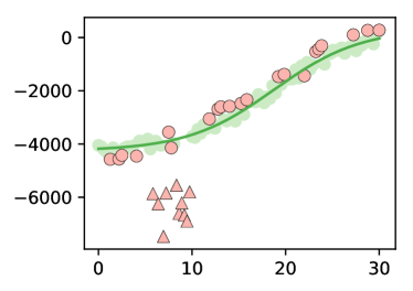
where $x\in\mathbb{R}^{4}$ represents the parameters of the model and $t\in\mathbb{R}$ represents the variable of the model. In order to generate random data for the test, the procedures detailed in Subsection 4.1 were used. The produced data is displayed in Figure 1, where $r=10$, $p=9$ and the exact solution was $x^{*}=(6000,-5000,-0.2,-3.7)$. This example has only $r-p=1$ outlier.

Figure 1: Test problem simulating an experiment following the logistic model. The continuous line represents the adjusted model, while the dashed line is the “exact” solution. LM-LOVO correctly identifies and ignores the outlier.

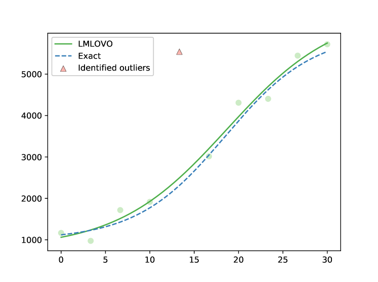
LM-LOVO was run with its default parameters, using $x=(0,0,0,0)$ as a starting point and $p=9$, indicating that there are 9 points which are trustable for adjusting the model. The solution found is also shown in Figure 1, given by $\bar{x}=(795.356,5749.86,0.161791,3.02475)$, as a continuous line, while the “exact” solution is depicted as a dashed line. We observe that it is not expected the exact solution $x^{*}$ to be found, since the points were perturbed. The outlier is correctly identified as the dark/red triangle.

The example in Figure 1 has an outlier that is visually easy to identify, so the correct number of $p=9$ trusted points was used. However, that might not be the case, specially if there is an automated process that needs to perform the adjustments, or if the model is multi-dimensional. Algorithm RAFF was implemented to solve this drawback.

RAFF was also implemented in the Julia language and is the main method of the RAFF.jl package [6]. As already mentioned in Section 2, RAFF is easily parallelizable, so serial and parallel/distributed versions are available, through the Distributed.jl package. The algorithm (or the user) defines an interval of values of $p$ to test and calls LM-LOVO to solve each subproblem for a given value of $p$. It is known that LOVO problems have many local minimizers, but we are strongly interested in global ones. Therefore, the traditional multi-start technique is applied to generate random starting points. The larger the number of different starting points, the greater is the chance to find global minimizers. Also, the computational cost is increased. The parallel/distributed version of RAFF solves this drawback, distributing problems with different values of $p$ among different cores, processors or even computers.

For the computation of the similarity between solutions $\bar{x}_{p}$ and $\bar{x}_{q}$ in Step 2, the Euclidean norm of the vector of differences was used

$$M_{pq}=\|\bar{x}_{p}-\bar{x}_{q}\|_{2}.$$

For each $p$ in the interval, the best solution $\bar{x}_{p}$ obtained among all the runs of LM-LOVO for that $p$ is stored. In order to avoid considering points in the cases where LM-LOVO has not converged for some value $p$, we set $M_{ip}=M_{pi}=\infty$ for all $i=p_{min},\dots,p_{max}$ in case of failure.

In the preprocessing phase (Step 2 of RAFF) solutions $\bar{x}_{q}$ that clearly are not minimizers are also eliminated by setting $M_{iq}=M_{qi}=\infty$ for all $i=p_{min},\dots,p_{max}$. To detect such points, we check if $S_{q}(\bar{x}_{q})>S_{p}(\bar{x}_{p})$ for some $q<p\leq p_{max}$. The idea is that the less points are considered in the adjustment, the smaller the residual should be at the global minimizer. The preprocessing phase also tries to eliminate solution $\bar{x}_{p_{max}}$. To do that, the valid solution $\bar{x}_{p}$ with smallest value of $S_{p}(\bar{x}_{p})$, which was not eliminated by the previous strategy, is chosen, where $p<p_{max}$. Solution $\bar{x}_{p_{max}}$ is eliminated if $S_{p}(\bar{x}_{p})<S_{p_{max}}(\bar{x}_{p_{max}})$ and the number of observed points $(t_{i},y_{i})$ such that $|y_{i}-\phi(\bar{x}_{p},t_{i})|<|y_{i}-\phi(\bar{x}_{p_{max}},t_{i})|$, for $i=1,\dots,r$, is greater or equal than $r/2$.

The last implementation detail of RAFF that needs to be addressed is the choice of $\epsilon$. Although this value can be provided by the user, we found very hard to select a number that resulted in a correct adjustment. Very small or very large values of $\epsilon$, result in the selection of $\bar{x}_{p_{max}}$ as the solution, since each solution will be similar to itself or similar to every solution, and we always select the largest $p$ in such cases. To solve this issue, the following calculation has been observed to work well in practice

$$\epsilon=\min(M)+\operatorname{avg}(M)/(1+p_{max}^{1/2}),$$ (21)

where $M$ is the similarity matrix and function $\operatorname{avg}$ computes the average similarity by considering only the lower triangular part of $M$ and ignoring $\infty$ values (which represent eliminated solutions). If there is no convergence for any value of $p\in[p_{min},p_{max}]$, then $\bar{x}_{p_{max}}$ is returned, regardless if it has successfully converged or not.

4.1 Experiments for outlier detection and robust fitting

In the first set of tests, we verified the ability and efficiency of RAFF to detect outliers for well known statistical and mathematical models:

• Linear model: $\phi(x,t)=x_{1}t+x_{2}$

• Cubic model: $\phi(x,t)=x_{1}t^{3}+x_{2}t^{2}+x_{3}t+x_{4}$

• Exponential model: $\phi(x,t)=x_{1}+x_{2}\exp(-x_{3}t)$

• Logistic model: $\phi(x,t)=x_{1}+\frac{x_{2}}{1+\exp(-x_{3}t+x_{4})}$

The large number of parameters to be adjusted increases the difficulty of the problem, since the number of local minima also increases. For these tests, we followed some ideas described in [18]. For each model, we created 1000 random generated problems having: 10 points and 1 outlier, 10 points and 2 outliers, 100 points and 1 outlier, and 100 points and 10 outliers. For each combination, we also tested the effect of the multistart strategy using: 1, 10, 100 and 1000 random starting points.

The procedure for generating each random instance is described as follows. It is also part of the RAFF.jl package [6]. Let $x^{*}$ be the exact solution for this fitting problem. First, $r$ uniformly spaced values for $t_{i}$ are selected in the interval $[1,30]$. Then, a set $O\subset\{1,\dots,r\}$ with $r-p$ elements values is randomly selected to be the set of outliers. For all $i=1,\dots,r$ a perturbed value is computed, simulating the results from an experiment. Therefore, we set $y_{i}=\phi(x^{*},t_{i})+\xi_{i}$, where $\xi_{i}\sim\operatorname{\mathcal{N}}(0,200)$, if $i\not\in O$ and, otherwise, $y_{i}=\phi(x^{*},t_{i})+7s\xi^{\prime}_{i}\xi_{i}$, where $\xi_{i}\sim\operatorname{\mathcal{N}}(0,200)$, $\xi^{\prime}_{i}$ a uniform random number between 1 and 2 and $s\in\{-1,1\}$ is randomly selected at the beginning of this process (so all outliers are in the “same side” of the curve). The exact solutions used to generate the instances are given in Table 1. The example illustrated in Figure 1 was also generated by this procedure.

Model	$x^{*}$
Linear	$(-200,1000)$
Cubic	$(0.5,-20,300,1000)$
Exponential	$(5000,4000,0.2)$
Logistic	$(6000,-5000,-0.2,-3.7)$

Table 1: Exact solutions used for each model in order to generate random instances.

The parallel version of RAFF was run with its default parameters on a Intel Xeon E3-1220 v3 3.10GHz with 4 cores and 16GB of RAM and Linux LUbuntu 18.04 operating system. The obtained results are displayed in Tables 2 and 3. In those tables, $r$ is the number of points representing the experiments, $p$ is the number of trusted points, FR is the ratio of problems in which all the outliers have been found (but other points may be declared as outliers), ER is the ratio of problems where exactly the $r-p$ outliers have been found, TP is the average number of correctly identified outliers, FP is the average number of incorrectly identified outliers, Avg. is the average number of points that have been declared as outliers by the algorithm and Time is the total CPU time in seconds to run all the 1000 tests, measured with the @elapsed Julia macro. By default, $p_{min}=0.5r$ and $p_{max}=r$ are set in the algorithm. The success criteria (20) of LM-LOVO was set to $\varepsilon=10^{-4}$, while $\overline{\lambda}$ was set to $2$. For each combination (Model, $r$, $p$) there are 4 rows in Tables 2 and 3, representing different numbers of multistart trials: 1, 10, 100 and 1000.

Type	$r$	$p$	FR	ER	TP	FP	Avg.	Time (s)
Linear	10	9	0.858	0.552	0.858	0.349	1.21	2.167
			0.859	0.554	0.859	0.347	1.21	3.511
			0.859	0.554	0.859	0.347	1.21	12.893
			0.859	0.554	0.859	0.347	1.21	89.285
		8	0.467	0.418	1.112	0.144	1.26	2.344
			0.467	0.417	1.112	0.145	1.26	3.596
			0.467	0.417	1.112	0.145	1.26	13.164
			0.467	0.417	1.112	0.145	1.26	88.684
	100	99	0.983	0.078	0.983	10.656	11.64	10.297
			0.982	0.074	0.982	10.655	11.64	42.091
			0.982	0.074	0.982	10.677	11.66	316.604
			0.982	0.075	0.982	10.682	11.66	3082.385
		90	0.916	0.069	9.858	6.768	16.63	9.799
			0.916	0.070	9.858	6.798	16.66	40.581
			0.915	0.070	9.854	6.782	16.64	317.722
			0.917	0.070	9.860	6.799	16.66	3099.536
Cubic	10	9	0.767	0.572	0.767	0.290	1.06	3.062
			0.810	0.563	0.810	0.371	1.18	4.111
			0.886	0.549	0.886	0.461	1.35	16.370
			0.886	0.545	0.886	0.465	1.35	126.554
		8	0.150	0.122	0.581	0.243	0.82	2.353
			0.333	0.282	0.894	0.202	1.10	4.221
			0.525	0.462	1.220	0.143	1.36	16.482
			0.533	0.469	1.232	0.142	1.37	126.088
	100	99	0.990	0.046	0.990	10.997	11.99	11.485
			0.991	0.041	0.991	11.351	12.34	51.548
			0.992	0.037	0.992	11.788	12.78	420.033
			0.993	0.036	0.993	11.706	12.70	4123.040
		90	0.945	0.064	9.838	6.941	16.78	11.325
			0.930	0.063	9.816	7.299	17.11	50.685
			0.941	0.063	9.835	7.584	17.42	414.084
			0.940	0.060	9.833	7.714	17.55	4042.454

Table 2: Results of RAFF for the detection of outliers for linear and cubic models. For each kind of problem, a multistart strategy was tested with 1, 10, 100 and 1000 random starting points.

Type	$r$	$p$	FR	ER	TP	FP	Avg.	Time (s)
Exponential	10	9	0.549	0.141	0.549	0.751	1.30	5.627
			0.698	0.463	0.698	0.354	1.05	17.289
			0.777	0.535	0.777	0.338	1.11	136.491
			0.822	0.581	0.822	0.306	1.13	1215.738
		8	0.213	0.080	0.771	0.459	1.23	4.417
			0.292	0.264	0.921	0.152	1.07	18.053
			0.406	0.367	1.138	0.148	1.29	138.862
			0.516	0.480	1.246	0.092	1.34	1245.882
	100	99	0.982	0.089	0.982	5.444	6.43	47.235
			0.992	0.046	0.992	10.673	11.66	392.884
			0.992	0.047	0.992	10.794	11.79	3521.630
			0.993	0.044	0.993	11.298	12.29	35418.130
		90	0.532	0.133	8.234	1.921	10.15	47.915
			0.972	0.060	9.946	7.181	17.13	384.544
			0.980	0.054	9.959	7.611	17.57	3389.777
			0.980	0.063	9.939	7.772	17.71	34121.028
Logistic	10	9	0.009	0.001	0.009	0.116	0.13	2.705
			0.245	0.156	0.245	0.419	0.66	3.714
			0.420	0.309	0.420	0.292	0.71	18.144
			0.524	0.364	0.524	0.279	0.80	150.310
		8	0.003	0.001	0.091	0.400	0.49	1.914
			0.032	0.028	0.396	0.369	0.77	3.932
			0.065	0.059	0.389	0.285	0.67	21.091
			0.167	0.143	0.559	0.203	0.76	175.915
	100	99	0.535	0.006	0.535	7.105	7.64	9.426
			0.536	0.012	0.536	11.754	12.29	34.022
			0.894	0.063	0.894	2.529	3.42	309.246
			0.929	0.095	0.929	5.276	6.21	2678.522
		90	0.002	0.000	4.345	3.295	7.64	9.459
			0.008	0.001	4.599	5.502	10.10	38.605
			0.432	0.001	6.551	4.629	11.18	319.713
			0.430	0.099	8.084	2.001	10.09	2774.727

Table 3: Results for RAFF for the detection of outliers for exponential and logistic models. For each kind of problem, a multistart strategy was tested with 1, 10, 100 and 1000 random starting points.

Some conclusions can be drawn from Tables 2 and 3. We can see that RAFF attains its best performance for outlier detection when the number of correct points is not small, even though the percentage of outliers is high. For the exponential and logistic models, we also can see clearly the effect of the multistart strategy in increasing the ratio of identified outliers. In problems with 100 experiments, we observe that in almost all the cases the number of outliers have been overestimated in average: although the ratio of outlier identification is high (FR), the ratio of runs where only the exact outliers have been detected (TR) is very low, being below 20% of the runs. For small test sets, this ratio increases up to 50%, but difficult models, such as the exponential and logistic, have very low ratios. However, as we can observe in Figure 2, the shape and the parameters of the model are clearly free from the influence of outliers. This observation suggests that maybe the perturbation added to all the values is causing the algorithm to detect correct points as outliers. The effect of the number of multi-start runs linearly increases the runtime of the algorithm, but is able to improve the adjustment, specially for the logistic model. The exponential model has an awkward behavior, where the ER ratio decreases when the number of multi-start runs increases, although the ratio of problems where all the outliers have been detected increases (FR). This might indicate that the tolerance (21) could be improved. We can also observe that the runtime of the exponential model is ten times higher than the other models.

When the size of the problem is multiplied by 10 (from 10 points to 100), we observe that the CPU time is multiplied by 5. This occurs because the time used by communication in the parallel runs is less important for larger datasets. Again, the exponential model is an exception.

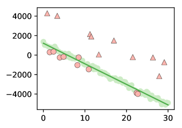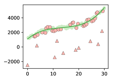Linear	Cubic
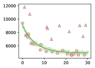Exponential	Logistic

Figure 2: Selected instances of test problems with $r=100$ and $p=90$ and the solutions obtained by RAFF. All the outliers have been correctly identified in those cases (dark/red triangles). Non-outliers are described by circles, where the dark/red ones represent points incorrectly classified as outliers by the algorithm.

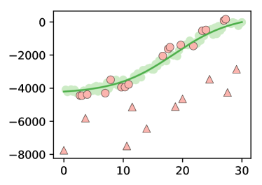
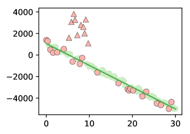
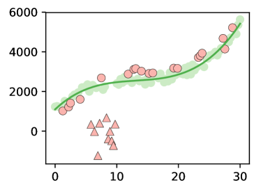
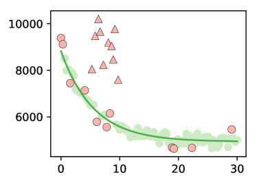
In a second round of experiments, the same procedure was used to generate random test problems simulating results from 100 experiments ($r=100$), where a cluster of 10% of the points are outliers ($p=90$). The default interval used for the values of $t$ is $[1,30]$, and the clustered outliers always belong to $[5,10]$. Selected instances for each type of model are shown in Figure 3 as well as the solution found by RAFF. Again, 1000 random problems were generated for each type of model and the multi-start procedure was fixed to 100 starting points for each problem. The obtained results are shown in Table 4. A clustered set of outliers can strongly affect the model but is also easier to detect, when the number of outliers is not very large. As we can observe in Table 4, the ratio of instances where all the outliers have been successfully detected has increased in all models. The logistic model is the most difficult to fit since, on average, RAFF detects 17 points as outliers and 9 of them are correctly classified (TP). All the other models are able to correctly identify 10 outliers, on average, and have a higher FR ratio.

This set of experiments also shows another benefit of the present approach. If the user roughly knows the number of points that belong to a given model, such information can be used in the elimination of random (not necessary Gaussian) noise. The clustered example will be also shown to be an advantage over traditional robust least-squares algorithms in Subsections 4.2 and 4.3.

Linear	Cubic
Exponential	Logistic

Figure 3: Selected instances of test problems containing a clustered set of outliers and the solutions obtained by RAFF. All the outliers have been correctly identified in those cases (dark/red triangles). Non-outliers are described by circles, where the dark/red ones represent points incorrectly classified as outliers by the algorithm.

Type	FR	ER	TP	FP	Avg.	Time (s)
Linear	0.949	0.104	9.936	6.363	16.30	323.623
Cubic	0.991	0.047	9.991	8.368	18.36	423.634
Exponential	0.987	0.097	9.983	6.775	16.76	3445.482
Logistic	0.745	0.007	8.778	8.382	17.16	326.675

Table 4: Numerical results for problems with $p=100$ data points and 10% of clustered outliers.

4.2 Comparison against robust algorithms

We compared the fitting obtained by RAFF against classical and robust fitting algorithms provided by the SciPy library version 1.3.1 in Python. The robust fitting algorithm in SciPy consists of using different loss functions in the least squares formulation. The following loss functions were used: linear (usual least squares formulation), soft_l1 (smooth approximation of the $\ell_{1}$ loss function), huber and cauchy. The PyCall.jl Julia library was used to load and call SciPy.

Two more algorithms based on the RANSAC (Random Sample Consensus) [9], implemented in C$++$ from the Theia Vision Library version 0.8, were considered. The first one, called here RANSAC, is the traditional version of RANSAC and the second one is LMED, based on the work [20], which does not need the error threshold, the opposite of case of RANSAC (where the threshold is problem dependent).

All the algorithms from SciPy were run with their default parameters. The best model among 100 runs was selected as the solution for each algorithm and the starting point used was randomly generated following the normal distribution with $\mu=0$ and $\sigma=1$. Algorithms RANSAC and LMED were run only 10 times, due to the higher CPU time used and the good quality of the solution achieved. RANSAC and LMED were run with a maximum of 1000 iterations, sampling 10% of the data and with the MLE score parameter activated. In order to adjust models to the sampled data, the Ceres least squares solver version 1.13.0 was used, since Theia has a natural interface to it. All the scripts used in the tests are available at https://github.com/fsobral/RAFF.jl. Once again, the parallel version of RAFF was used. The test problems were generated by the same procedures discussed in Subsection 4.1. However, only one problem (instead of 1000) for each configuration (Model, $r$, $p$) was used.

Unlike RAFF, traditional fitting algorithms do not return the possible outliers of a dataset. Robust algorithms such as least squares using $\ell_{1}$ or Huber loss functions are able to ignore the effect of outliers, but not to easily detect them. Therefore, for the tests we selected one instance of each test of type (model, $r$, $p$), where the models and values for $r$ and $p$ are the same used in Tables 2–4. The results are displayed in Table 5. For each problem $p$ and each algorithm $a$, we measured the adjustment error $A_{a,p}$ between the model obtained by the algorithm $\phi_{p}(x_{a,p}^{\star},t)$ and the points that are non-outliers, which is given by

$$A_{a,p}=\sqrt{\sum\limits_{\begin{subarray}{c}i\in\mathcal{P}\\ i\ \mbox{non-outlier}\end{subarray}}(\phi_{p}(x_{a,p}^{\star},t_{i})-y_{i})^{2}},$$

where $\phi_{p}$ was the model used to adjust problem $p$. Each row of Table 5 represents one problem and contains the relative adjustment error for each algorithm, which is defined by

$$\bar{A}_{a,p}=\frac{A_{a,p}}{\min_{i}\{A_{i,p}\}}$$ (22)

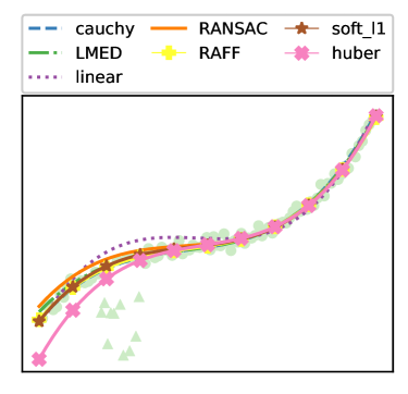
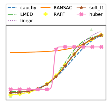
and the time taken to find the model (in parenthesis). The last row contains the number of times that each algorithm has found a solution with adjustment error smaller than 1% of best, smaller than 10% of the best and smaller than 20% of the best adjustment measure found for that algorithm, respectively, in all the test set. We can observe that RAFF, LMED and soft_l1 were the best algorithms. RAFF was the solver that found the best models in most of the problems (11/24), followed by LMED (9/24). Its parallel version was consistently the fastest solver among all. It is important to observe that RAFF was the only who was easily adapted to run in parallel. However, the parallelism is related only to the solution of subproblems for different $p$, not to the multistart runs, which are run sequentially. Therefore, RAFF solves considerably more problems per core than the other algorithms in a very competitive CPU time. When parallelism is turned of, the CPU time is very similar to the traditional least squares algorithm (linear). Also, RAFF was the only one that easily outputs the list of possible outliers without the need of any threshold parameter. Clustered instance (cubic, 100, 90) and instance (logistic, 10, 9) and the models obtained by each algorithm are shown in Figure 4.

(Model, $r$, $p$)	linear	soft_l1	huber	cauchy	RANSAC	LMED	RAFF
linear, 10, 9	1.35 ( 0.60)	1.06 ( 2.75)	1.06 ( 3.11)	1.37 ( 1.64)	4.28 ( 0.52)	1.00 ( 0.53)	1.35 ( 1.48)
linear, 10, 8	3.62 ( 0.60)	1.18 ( 2.55)	1.18 ( 2.89)	1.14 ( 2.07)	1.17 ( 0.54)	1.01 ( 0.55)	1.00 ( 0.12)
linear, 100, 99	1.03 ( 0.60)	1.00 ( 3.22)	1.00 ( 8.43)	1.00 ( 2.30)	1.22 ( 3.95)	1.00 ( 3.98)	1.00 ( 0.82)
linear, 100, 90	1.75 ( 0.60)	1.00 ( 3.41)	1.00 ( 8.41)	1.04 ( 1.65)	1.23 ( 4.71)	1.01 ( 47.23)	1.04 ( 0.67)
cubic, 10, 9	1.27 ( 0.81)	1.00 ( 9.44)	1.11 ( 11.42)	4.71 ( 4.67)	22.26 ( 0.98)	2.47 ( 0.99)	4.91 ( 1.04)
cubic, 10, 8	4.06 ( 0.73)	1.18 ( 14.80)	1.18 ( 16.28)	1.19 ( 4.75)	114.88 ( 1.00)	1.21 ( 1.00)	1.00 ( 0.18)
cubic, 100, 99	1.05 ( 0.72)	1.00 ( 21.08)	2.24 ( 22.20)	1.09 ( 6.00)	1.12 ( 8.00)	1.04 ( 8.04)	1.08 ( 0.81)
cubic, 100, 90	1.76 ( 0.73)	1.00 ( 21.59)	1.78 ( 22.86)	1.19 ( 5.79)	1.15 ( 7.94)	1.00 ( 79.15)	1.00 ( 0.75)
expon, 10, 9	1.16 ( 5.04)	12.88 ( 12.26)	12.88 ( 12.59)	4.68 ( 10.70)	14.22 ( 0.76)	1.00 ( 0.76)	1.16 ( 1.35)
expon, 10, 8	1.34 ( 3.28)	7.74 ( 12.14)	10.07 ( 12.45)	1.00 ( 10.89)	1.72 ( 0.72)	1.61 ( 0.73)	1.34 ( 0.25)
expon, 100, 99	1.00 ( 3.86)	8.57 ( 13.61)	8.58 ( 12.86)	1.22 ( 10.99)	2.04 ( 5.32)	1.05 ( 5.32)	1.03 ( 5.19)
expon, 100, 90	1.76 ( 3.65)	8.99 ( 13.53)	8.99 ( 13.18)	3.70 ( 11.04)	1.93 ( 5.35)	1.00 ( 53.63)	1.02 ( 5.32)
logistic, 10, 9	1.68 ( 3.24)	1.31 ( 18.98)	7.60 ( 20.55)	1.91 ( 17.28)	24.45 ( 0.89)	2.27 ( 0.90)	1.00 ( 0.99)
logistic, 10, 8	4.23 ( 10.27)	1.00 ( 18.14)	9.40 ( 19.18)	26.13 ( 3.98)	39.56 ( 0.85)	1.05 ( 0.87)	22.19 ( 0.14)
logistic, 100, 99	1.01 ( 4.44)	2.34 ( 17.68)	8.88 ( 18.84)	2.64 ( 8.24)	1.02 ( 7.75)	1.00 ( 7.76)	1.01 ( 0.51)
logistic, 100, 90	1.78 ( 2.57)	1.10 ( 18.16)	7.13 ( 19.10)	7.53 ( 8.06)	1.06 ( 7.59)	1.00 ( 76.37)	1.01 ( 0.53)
Clustered
linear, 10, 8	4.10 ( 0.52)	1.18 ( 2.33)	1.18 ( 2.54)	1.00 ( 2.02)	4.69 ( 0.54)	1.07 ( 0.55)	1.00 ( 0.10)
linear, 100, 90	1.92 ( 0.62)	1.00 ( 2.76)	1.00 ( 5.70)	1.12 ( 2.10)	1.11 ( 4.66)	1.02 ( 46.45)	1.03 ( 0.68)
cubic, 10, 8	4.29 ( 0.72)	1.00 ( 11.90)	1.00 ( 14.59)	11.59 ( 4.87)	31.72 ( 1.04)	10.79 ( 1.02)	12.61 ( 0.14)
cubic, 100, 90	2.18 ( 0.73)	1.02 ( 20.39)	2.47 ( 22.25)	1.07 ( 6.31)	1.52 ( 7.70)	1.09 ( 73.61)	1.00 ( 0.83)
expon, 10, 8	1.32 ( 12.79)	4.11 ( 10.54)	1.81 ( 10.34)	1.20 ( 9.18)	1.00 ( 0.75)	2.69 ( 0.78)	4.22 ( 0.29)
expon, 100, 90	1.99 ( 3.56)	8.58 ( 13.31)	8.57 ( 12.79)	4.99 ( 10.90)	1.74 ( 5.66)	1.14 ( 57.14)	1.00 ( 5.82)
logistic, 10, 8	3.79 ( 10.17)	1.00 ( 15.28)	7.74 ( 18.09)	22.46 ( 10.53)	16.32 ( 0.66)	1.40 ( 0.65)	12.31 ( 0.13)
logistic, 100, 90	2.00 ( 4.87)	4.62 ( 18.10)	6.77 ( 19.83)	7.35 ( 7.10)	1.40 ( 7.78)	1.03 ( 78.43)	1.00 ( 0.52)
	2, 5, 6	9, 11, 15	4, 5, 9	3, 6, 11	1, 3, 7	9, 16, 17	11, 16, 17

Table 5: Comparison against different robust fitting algorithms using one instance of each test problem and 100 random starting points as a multistart strategy. RANSAC and LMED run for 10 random initial points.

Figure 4: Two problems and the models found for each algorithm. On the left, a cubic model with 100 points and a set of 10 clustered outliers. On the right, a logistic model with 10 points and only one outlier.

4.3 Experiments for circle detection

The problem of detecting patterns in images is very discussed in the vision area in Computer Science. LOVO algorithms have also been applied to solving such problems, as a nonlinear programming alternative to traditional techniques [1]. The drawback, again, is the necessity of providing a reasonable number of trusted points. RAFF allows the user to provide an interval of possible trusted points, so the algorithm can efficiently save computational effort when trying to find patterns in images. Since LOVO problems need a model to be provided, circle detection is a perfect application to the algorithm.

We followed tests similar to [24], using a circular model

$$\phi(x,t)=(t_{1}-x_{1})^{2}+(t_{2}-x_{2})^{2}-x_{3}^{2}$$

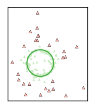
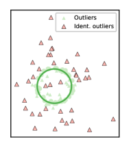
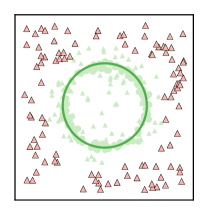
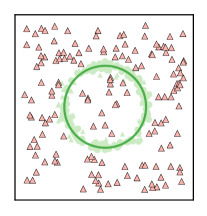
instead of the ellipse model considered in the work. Two test sets were generated. In the first set $r=100$ points were uniformly distributed in the border of the circle with center $(-10,30)$ and radius $2$. If the point is not an outlier, a random perturbation $\xi\sim\operatorname{\mathcal{N}}(0,0.1)$ is added to each one of its $t_{1}$ and $t_{2}$ coordinates. For outliers, the random noise is given by $\xi\sim\operatorname{\mathcal{N}}(0,2)$, as suggested in [24]. In the second set, $r=300$ was considered. The same circumference was used and $p$ points (non-outliers) were uniformly distributed in the circumference and slightly perturbed with a noise $\xi\sim\operatorname{\mathcal{N}}(0,0.1)$ as before. The remaining $300-p$ points (the outliers) were randomly distributed in a square whose side was 4 times the radius of the circle, using the uniform distribution. Nine problems were generated in each test set, with outlier ratio ranging from 10% up to 90% (i. e. ratio of non-outliers decreasing 90% to 10%).

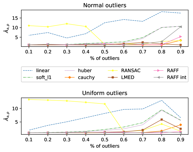
The same algorithms were compared, the only difference from Subsection 4.2 is that the error threshold of RANSAC was reduced to 10 and 100 random starting points near $(1,1,1)$ were used for all algorithms, except RANSAC and LMED. For those two algorithms, we kept the number of trials to 10. Also, we tested two versions of RAFF. In pure RAFF, we decreased the lower bound $p_{min}$ from its default value $0.5r$ to the value of $p$, when $p$ falls below the default. In RAFFint, we used the option of providing upper and lower bounds for the number of trusted points. If $p$ is the current number of non-outliers in the instance, the interval given to RAFFint is $[p-0.3r,p+0.3r]\cap[0,r]$. The measure (22) was used and the results are shown in Figure 5.

We can observe that RAFF, LMED and cauchy achieved the best results. RAFF found worse models than most of the robust algorithms in the problems of the first test set, although the results are still very close. Its relative performance increases as the outlier ratio increases. This can be explained as the strong attraction that RAFF has to finding a solution similar to traditional least squares algorithms. In Figure 6 we can see that RAFF has difficulty in finding outliers that belong to the interior of the circle. To solve this drawback, RAFF also accepts a lower bound in the number of outliers, rather than only an upper bound. This ability is useful for large datasets with a lot of noise, as is the case of the second test set, and allows the detection of inner outliers. This is represented by RAFFint. We can see in Figure 5 that the performance of both versions of RAFF is better than traditional robust algorithms in the case of a large number of outliers.

Figure 5: Relative adjustment error in the circle detection problem for increasing outlier ratio and two different types of perturbation: by normal and uniform distributions.

Outliers generated by normal distribution
At most 40% of outliers	Outlier ratio between 10% and 60%
Outliers generated by uniform distribution
At most 40% of outliers	Outlier ratio between 20% and 60%

Figure 6: Difference of outlier detection when upper bounds on the outlier ratio are provided. The inner outliers are harder to detect, since the error they cause in the model is smaller.

5 Conclusions

In this paper, we have described a LOVO version of the Levenberg-Marquardt algorithm for solving nonlinear equations, which is specialized to the adjustment of models where the data contains outliers. The theoretical properties of the algorithm were studied and convergence to weakly stationary points has been proved. To overcome the necessity of providing the number of outliers in the algorithm, a voting system has been proposed. A complete framework to robust adjustment of data was implemented in the Julia language and compared to public available and well tested robust fitting algorithms. The proposed algorithm was shown to be competitive, being able to find better adjusted models in the presence of outliers in most of the problems. In the circle detection problem, the proposed algorithm was also shown to be competitive and had a good performance even when the outlier ration exceeds 50%. The implemented algorithm and all the scripts used for testing and generation of the tests are freely available and constantly updated at https://github.com/fsobral/RAFF.jl.

References

- [1] R. Andreani, G. Cesar, R. Cesar-Jr., J. M. Martínez, and P. J. S. Silva. Efficient curve detection using a Gauss-Newton method with applications in agriculture. In Proc. 1st International Workshop on Computer Vision Applications for Developing Regions in Conjunction with ICCV 2007-CVDR-ICCV07, 2007.
- [2] R. Andreani, J. M. Martínez, L. Martínez, and F. S. Yano. Continuous optimization methods for structure alignments. Mathematical Programming, 112(1):93–124, 2008.
- [3] R. Andreani, J. M. Martínez, L. Martínez, and F. S. Yano. Low Order-Value Optimization and applications. Journal of Global Optimization, 43(1):1–22, 2009.
- [4] E. Bergou, Y. Diouane, and V. Kungurtsev. Convergence and iteration complexity analysis of a Levenberg-Marquardt algorithm for zero and non-zero residual inverse problems, 2018.
- [5] E. G. Birgin, L. F. Bueno, N. Krejić, and J. M. Martínez. Low Order-Value approach for solving VaR-constrained optimization problems. Journal of Global Optimization, 51(4):715–742, 2011.
- [6] E. V. Castelani, R. Lopes, W. Shirabayashi, and F. N. C. Sobral. RAFF.jl: Robust Algebraic Fitting Function in Julia. Journal of Open Source Software, 4(39):1385, 2019.
- [7] R. D. Cook. Detection of influential observations in linear regression. Technometrics, 19:15–18, 1977.
- [8] R. O. Duda and P. E. Hart. Use of the Hough transformation to detect lines and curves in pictures. Technical report, Sri International Menlo Park Ca Artificial Intelligence Center, 1971.
- [9] M. A. Fischler and R. C. Bolles. Random sample consensus: a paradigm for model fitting with applications to image analysis and automated cartography. Communications of the ACM, 24(6):381–395, 1981.
- [10] F. R. Hampel, E. Ronchetti, P. Rousseeuw, and W. Stahel. Robust Statistics: The Approach Based on Influence Functions. John Wiley & Sons, New York, NY, USA, 1986.
- [11] V. Hodge and J. Austin. A survey of outlier detection methodologies. Artificial Intelligence Review, 22(2):85–126, 2004.
- [12] P. V. Hough. Method and means for recognizing complex patterns, Dec. 18 1962. US Patent 3,069,654.
- [13] J. Illingworth and J. Kittler. A survey of the Hough transform. Computer vision, graphics, and image processing, 44(1):87–116, 1988.
- [14] Z. Jiang, Q. Hu, and X. Zheng. Optimality condition and complexity of Order-Value Optimization problems and Low Order-Value Optimization problems. Journal of Global Optimization, 69(2):511–523, 2017.
- [15] J. M. Martínez. Generalized order-value optimization. TOP, 20(1):75–98, 2012.
- [16] L. Martínez, R. Andreani, and J. M. Martínez. Convergent algorithms for protein structural alignment. BMC Bioinformatics, 8(1):306, 2007.
- [17] J. J. Moré. The Levenberg-Marquardt algorithm: implementation and theory. In Numerical analysis, pages 105–116. Springer Berlin Heidelberg, 1978.
- [18] H. J. Motulsky and E. R. Brown. Detecting outliers when fitting data with nonlinear regression – a new method based on robust nonlinear regression and the false discovery rate. BMC Bioinformatics, 7(123), 2006.
- [19] J. Nocedal and S. J. Wright. Numerical Optimization. Springer, New York, 2nd edition, 2006.
- [20] P. J. Rousseeuw. Least median of squares regression. Journal of the American Statistical Association, 79(388):871–880, 1984.
- [21] R. E. Shiffler. Maximum Z scores and outiliers. The American Statistics, 42(1):79–80, 1988.
- [22] S. S. Sreevidya. A survey on outlier detection methods. International Journal of Computer Science and Information Technologies, 5(6):8153–8156, 2014.
- [23] L. Xu, E. Oja, and P. Kultanen. A new curve detection method: randomized Hough transform (RHT). Pattern recognition letters, 11(5):331–338, 1990.
- [24] J. Yu, H. Zheng, S. R. Kulkarni, and H. Poor. Two-stage outlier elimination for robust curve and surface fitting. EURASIP Journal on Advances in Signal Processing, 2010(1), 2010.