Abstract

In this lectures, we give a review about the Minimal Supersymmetric Standard Model (MSSM) and the General Singlet Extensions of the MSSM (GSEMSSM). We, first introduce the minimal set of fields to built both models. Then we introduce their superfields and using them we build the lagrangian of those models in the superspace formalism. We show how to get the mass spectrum of those model in the $R$-parity scenarios and we also show how to get some Feynman Rules with the Gauge Bosons. The second part of this review was presented at Dark Mattter Workshop – Early Universe Cosmology, Baryogenesis and Dark Matter held in Instituto de Física Teória (IFT-Unesp) from 21 to 25 of October 2019.

PACS number(s): 12.60. Jv

Keywords: Supersymmetric Models

1 Introduction

Although the Standard Model (SM) describes the observed properties of charged leptons and quarks. The success of the SM has been astonishing. Nevertheless, the SM is not considered as the ultimate theory since neither the fundamental parameters, masses and couplings, nor the symmetry pattern are predicted.

It is commonly agreed that the Higgs sector of the SM is unsatisfactory. One of this reason is the hierarchy problem. When we define the Higgs potential, we need to define the squared mass parameter $\mu^{2}$, this is a free parameter and it is not fixed by the theory. The Higgs potential is defined as

$$V(H)=-\mu^{2}|H|^{2}+\lambda\left(|H|^{2}\right)^{2}.$$ (1)

In the SM there is only one physical neutral Higgs scalar in the spectrum, and its mass is given by [2]

$$M_{H}=\sqrt{2}\mu.$$ (2)

The SM is renormalizable, wchich means that finite results are obtained for all higher-order (loop) corrections even if we extend the virtual momenta in the loop integral all the way to infinity. The 4-boson self interaction in Eq.(1) generate, at one loop order, the self-energy, wchich is proportional to [2]

$$\lambda\int^{\Lambda}d^{4}k\frac{1}{k^{2}-M^{2}_{H}}.$$ (3)

The coefficient $\mu$ is then replaced by the one loop-corrected ‘ ‘physical” value $\mu_{\mbox{ phys}}$ where

$$\mu^{2}_{\mbox{ phys}}=\mu^{2}-\lambda\Lambda^{2},$$ (4)

The parameter $\Lambda$ is the energy scale wehere we expect to find the physics beyond the SM, in GUT scenarios we expect $\Lambda\sim M_{Pl}\approx 10^{19}$ GeV, the one loop correction is then vastly greater than $M_{W}\approx\left(100\mbox{GeV}\right)^{2}$ and it is known as hierachy problem. It means, the hierarchy problem [1] is to understand why $M_{H}$, given at Eq.(2), is much less then the Planck mass Scale $M_{Pl}$.

It is clearly prudent to explore the implication of more complicated Higgs Models, both in the context of SM and in extended theories. Although the minimal Higgs satisfy [2]

$$\rho=\frac{M_{W}}{M_{Z}\cos\theta_{W}}\approx 1,$$ (5)

so does any version of the SM with any number of the Higgs doublets, one example is the Two Higgs Doublet Model (THM) [2, 3, 4, 5, 6, 7, 8, 9], (and singlets [10, 11]), for more details about this interesting problem see [2, 12, 13]. But unfortunatelly the THM can not solve the hierachy problem, for more details about this fact see [2].

One intersting class of models to be the physics beyond the SM is Supersymmetry, it is more known as SUSY [14]. The hierachy can be solved in Supersymmetric Model, known as SUSY by short [15, 16, 17]. The supersymmetry automatically cancels all quadratic corrections in all orders of perturbation theory due to the contributions of superpartners of the ordinary particles.

The most intensively studied model is the Minimal Supersymmetric Standard Model (MSSM) [20, 21, 22], which is the most economical realization of SUSY. Control of the radiative corrections so that a small value of $\mu^{2}$ (and hence $M^{2}_{H}$ and $M^{2}_{W}$) becomes natural was a primary motivation of the MSSM where we show the exact cancelation to the Higgs masses coming from fermion contribution. A light Higgs sector ($M^{2}_{H}\ll M^{2}_{Pl}$) is natural in a softly broken SUSY scenarios where the quadratically divergent loop contribution cancel leaving a finite correction of the form

$$\delta M^{2}_{H}={\cal O}\left(\frac{\alpha}{\pi}\right)\left(M^{2}_{B}-M^{2}_{F}\right),$$ (6)

where $M_{B,F}$ are the masses of the bosonic and fermionic partner particles circulating in the loops. When we consider scenarios with soft SUSY breakings terms we have the following constraints

$$M^{2}_{B}-M^{2}_{F}\simeq{\cal O}(M_{W})=M_{SUSY}^{2},$$ (7)

which should not be very large ($\leq$ 1 TeV) to make the fine-tuning natural. Therefore, it provides a solution to the hierarchy problem by protecting the eletroweak scale from large radiative corrections [23, 24]. However, the origin of the hierarchy is the other part of the problem.

SUSY arose in theoretical papers more than 30 years ago independently and the originals works were made by the following set of authors:

• Golfand and Likhtman [26];

• Volkov and Akulov [27];

• Wess and Zumino [28, 29].

Some very nices reviews about the begining of SUSY can be found in the following references [30, 31, 32].

SUSY, is basically a symmetry between bosons (particles with integer spin) and fermions (particles with half-integer spin) [15, 16, 17]. Since that time there appeared thousands of papers and the reason for this remarkable is due the fact that there are a number of theoretical and phenomenological issues that the SM fails to address adequately [33, 34, 35, 36, 37, 38, 39]:

• Unification with gravity; The point is that SUSY algebra being a generalization of Poincaré algebra [16, 34, 35, 36]

  $$\{Q_{\alpha},\bar{Q}_{\dot{\alpha}}\}=2\sigma_{\alpha,\dot{\alpha}}^{m}P_{m}.$$ (8)

  Therefore, when we make SUSY local, one obtains supergravity [41].

• Unification of Gauge Couplings; According to hypothesis of Grand Unification Theory (GUT) all gauge couplings change with energy. In the MSSM the slopes of Renormalization Group Equation (RGE) curves about the running of behaviour of gauge couplings can achieve perfect unification [42].

• Hierarchy problem (discussed above);

• Electroweak symmetry breaking (EWSB); The “running” of the Higgs masses, using the RGE of MSSM, leads to the phenomenon known as radiative electroweak symmetry breaking. Indeed, the mass parameters from the Higgs potential $m_{1}^{2}$ and $m_{2}^{2}$ (or one of them) decrease while running from the GUT scale to the scale $M_{Z}$ may even change the sign. Thus the breaking of the electroweak symmetry is not introduced by brute force as in the SM, but appears naturally from the radiative corrections [43].

The main sucess of SUSY is to solve all the problems listed above. However, SUSY has also made several correct predictions [33]:

• SUSY predicted in the early 1980s that the top quark would be heavy [44, 45], its experimental value is given by $m_{t}=172.25\pm 0.08\mathrm{(stat.)}\pm 0.62\mathrm{(syst.)}~{}\mathrm{GeV}$ [46];

• SUSY GUT theories with a high fundamental scale accurately predicted the present experimental value of $\sin^{2}\theta_{W}$ before it was mesured [47, 48, 49, 50];

• SUSY requires a light Higgs boson to exist [23, 24, 51, 52, 53, 54, 55], its experimental value is $M_{H}=125.09\pm 0.21\,\mathrm{(stat.)}\pm 0.11\,\mathrm{(syst.)}~{}\mathrm{GeV}$ [56].

Together these success provide powerful indirect evidence that low energy SUSY is indeed part of correct description of nature. The MSSM [20, 21, 22, 34, 35, 36, 37, 38, 39] have, also viable candidates to be the Dark Matter on this case it can be the lightest neutralino, lighest sneutrino and the gravitino, more details about SUSY Dark Matter Candidates is presented in nice way in [59].

However, the MSSM suffers from the $\mu$-problem. The $\mu$-parameter is the only dimensional parameter in the SUSY conserving sector and one would expect the $\mu$ to be either zero or at the Planck scale. A simple solution is to promote $\mu$ to a dynamical field in extensions of the MSSM that contain an additional singlet superfield $\hat{S}$ which does not interact with the MSSM fields other than the two Higgs doublets, it is a singlet. An effective $\mu$ can be reasonably got at Electro-Weak scale when $\hat{S}$ denotes the vacuum expectation value (VEV) of the singlet scalar field. Among these extension models the Next-to-Minimal Supersymmetric Model (NMSSM) [20, 60, 61, 62, 63, 64, 65, 66, 67, 68, 69].

If introduce a singlet superfield to the MSSM, the Higgs sector will have one more CP even component and one more CP odd component, and the neutralino sector will have one more singlino component. These singlet multiplets compose a “singlet sector” of the MSSM, the nearly Minimal Supersymmetric Model (nMSM) [121, 122] and the General Singlet Extensions of the MSSM (GSEMSSM). It can make the phenomenologies of SUSY dark matter and Higgs different from the MSSM, and it can get some interesting cosmological consequences as discussed recently [10, 11].

As in our opinion, the MSSM and GSEMSSM are good candidates to be the extension of the SM we will on this review present those models in some details inclunding some numerical analyses.

2 Superfields

The superfield formalism was formulated in independent way by

• A. Salam and J. Strathdee [70];

• S. Ferrara, J. Wess and B. Zumino [71].

The most general superfield is given by [16, 17, 34, 35, 36, 77]:

$${\cal F}(x,\theta,\bar{\theta}) = f(x)+\left(\theta\phi(x)\right)+\left(\bar{\theta}\bar{\chi}(x)\right)+\left(\theta\theta\right)m(x)+\left(\bar{\theta}\bar{\theta}\right)n(x)+\left(\theta\sigma^{m}\bar{\theta}\right)v_{m}(x)$$ (9)

$$+ \left(\theta\theta\right)\left(\bar{\theta}\bar{\lambda}(x)\right)+\left(\bar{\theta}\bar{\theta}\right)\left(\theta\psi(x)\right)+\left(\theta\theta\right)\left(\bar{\theta}\bar{\theta}\right)d(x),$$

where

$$f(x),\,\ m(x),\,\ n(x),\,\ d(x),\,\ {\mbox{s}calars},$$

$$\phi(x),\,\ \psi(x),\,\ \bar{\chi}(x),\,\ \bar{\lambda}(x),\,\ {\mbox{s}pinors},$$

$$v_{m}(x),\,\ {\mbox{v}ector}.$$ (10)

The infinitesimal variation of the general superfield under supersymmetric transformation, are given by:

$$\delta_{\xi}{\cal F}(x,\theta,\bar{\theta}) = \delta_{\xi}f(x)+\left(\theta\delta_{\xi}\phi(x)\right)+\left(\bar{\theta}\delta_{\xi}\bar{\chi}(x)\right)+\left(\theta\theta\right)\delta_{\xi}m(x)+\left(\bar{\theta}\bar{\theta}\right)\delta_{\xi}n(x)+\left(\theta\sigma^{m}\bar{\theta}\right)\delta_{\xi}v_{m}(x)$$

$$+ \left(\theta\theta\right)\left(\bar{\theta}\delta_{\xi}\bar{\lambda}(x)\right)+\left(\bar{\theta}\bar{\theta}\right)\left(\theta\delta_{\xi}\psi(x)\right)+\left(\theta\theta\right)\left(\bar{\theta}\bar{\theta}\right)\delta_{\xi}d(x)$$

$$\equiv (\xi Q+\bar{\xi}\bar{Q}){\cal F}(x,\theta,\bar{\theta})\quad.$$

Using the Fierz identities, we then have that the component fields of ${\cal F}$ transform as follows:

$$\delta_{\xi}f = \xi\phi+\bar{\xi}\bar{\chi}\quad,$$

$$\delta_{\xi}\phi_{\alpha} = 2\xi_{\alpha}m+\sigma^{m}_{\alpha\dot{\beta}}\bar{\xi}^{\dot{\beta}}\left[\imath\left(\partial_{m}f\right)+v_{m}\right]\quad,$$

$$\delta_{\xi}\bar{\chi}^{\dot{\alpha}} = 2\bar{\xi}^{\dot{\alpha}}n+\xi^{\beta}\sigma^{m}_{\beta\dot{\gamma}}\epsilon^{\dot{\gamma}\dot{\alpha}}\left[\imath\left(\partial_{m}f\right)-v_{m}\right]\quad,$$

$$\delta_{\xi}m = \bar{\xi}\bar{\lambda}-\frac{\imath}{2}\left[\left(\partial_{m}\phi\right)\sigma^{m}\bar{\xi}\right]\quad,$$

$$\delta_{\xi}n = \xi\psi+\frac{\imath}{2}\left[\xi\sigma^{m}\left(\partial_{m}\bar{\chi}\right)\right]\quad,$$ (11)

$$\delta_{\xi}v_{m} = \left(\xi\sigma_{m}\bar{\lambda}\right)+\left(\psi\sigma_{m}\bar{\xi}\right)+\frac{\imath}{2}\left[\xi\left(\partial_{m}\phi\right)\right]-\frac{\imath}{2}\left[\left(\partial_{m}\bar{\chi}\right)\bar{\xi}\right]\quad,$$

$$\delta_{\xi}\bar{\lambda}^{\dot{\alpha}} = 2\bar{\xi}^{\dot{\alpha}}d+\frac{\imath}{2}\bar{\xi}^{\dot{\alpha}}\left(\partial^{m}v_{m}\right)+\imath(\xi\sigma^{m}\epsilon)^{\dot{\alpha}}\left(\partial_{m}m\right)\quad,$$

$$\delta_{\xi}\psi_{\alpha} = 2\xi_{\alpha}d-\frac{\imath}{2}\xi_{\alpha}\left(\partial^{m}v_{m}\right)+\imath(\sigma^{m}\bar{\xi})_{\alpha}\left(\partial_{m}n\right)\quad,$$

$$\delta_{\xi}d = \frac{\imath}{2}\partial_{m}\left[\left(\psi\sigma^{m}\bar{\xi}\right)+\left(\xi\sigma^{m}\bar{\lambda}\right)\right]\quad.$$

Note the important fact that the complex scalar component field $d(x)$ transforms by a total derivative.

The covariant derivative and it is given by[16, 17]

$$D_{\alpha} = \frac{\partial}{\partial\theta^{\alpha}}+i\sigma^{m}_{\alpha\dot{\alpha}}\bar{\theta}^{\dot{\alpha}}\frac{\partial}{\partial x^{m}}\,\$$

$$\bar{D}_{\dot{\alpha}} = -\frac{\partial}{\partial\bar{\theta}^{\dot{\alpha}}}-i\theta^{\alpha}\sigma^{m}_{\alpha\dot{\alpha}}\frac{\partial}{\partial x^{m}}\,\ .$$ (12)

and $\alpha=1,2$ is a spinorial index.

We know that the chiral superfield, denoted as ($\Phi$), and the anti-chiral, given by ($\bar{\Phi}$), has the following expansion[16, 17]

$$\Phi(y,\theta) = A(y)+\sqrt{2}\left(\theta\psi(y)\right)+\left(\theta\theta\right)F(y),\,\ \left(\theta\psi\right)\equiv\theta^{\alpha}\psi_{\alpha},\,\ \alpha=1,2,$$

$$\bar{\Phi}(\bar{y},\bar{\theta}) = A^{\dagger}(\bar{y})+\sqrt{2}\left(\bar{\theta}\bar{\psi}(\bar{y})\right)+\left(\bar{\theta}\bar{\theta}\right)F^{\dagger}(\bar{y}),\,\ \left(\bar{\theta}\bar{\psi}\right)\equiv\bar{\theta}_{\dot{\alpha}}\bar{\psi}^{\dot{\alpha}},\,\ \dot{\alpha}=1,2,$$ (13)

respectivelly and $A$ is a scalar field, $\psi$ is a Weyl-van der Waerden fermions field [16, 17, 73, 19] and $F$ is an scalar necessary to close the SUSY algebra [16, 17]. The new coordinate $y$ is defined as

$$y^{m} = x^{m}+\imath\left(\theta\sigma^{m}\bar{\theta}\right),$$ (14)

and $\bar{y}$ is the conjugate complex of $y$ defined above.

The superpotential $W$ is defined in general in the following way

$$W\equiv\lambda_{i}\Phi_{i}+\mu_{ij}\Phi_{i}\Phi_{j}+f_{ijk}\Phi_{i}\Phi_{j}\Phi_{k},$$ (15)

in terms of the fields components, see Eq.(13), can be written as [16, 17]

$$\Phi_{i}(y,\theta)\Phi_{j}(y,\theta) = A_{i}(y)A_{j}(y)+\sqrt{2}\theta\left[\psi_{i}(y)A_{j}(y)+A_{i}(y)\psi_{j}(y)\right]$$

$$+ \theta\theta\left[A_{i}(y)F_{j}(y)+F_{i}(y)A_{j}(y)-\psi_{i}(y)\psi_{j}(y)\right]$$

$$\Phi_{i}(y,\theta)\Phi_{j}(y,\theta)\Phi_{k}(y,\theta) = A_{i}(y)A_{j}(y)A_{k}(y)$$

$$+ \sqrt{2}\theta\left[\psi_{i}(y)A_{j}(y)A_{k}(y)+A_{i}(y)\psi_{j}(y)A_{k}(y)+A_{i}(y)A_{j}(y)\psi_{k}(y)\right]$$

$$+ \theta\theta\left[F_{i}(y)A_{j}(y)A_{k}(y)+A_{i}(y)F_{j}(y)A_{k}(y)+A_{i}(y)A_{j}(y)F_{k}(y)\right.$$

$$- \left.\psi_{i}(y)\psi_{j}(y)A_{k}(y)-A_{i}(y)\psi_{j}(y)\psi_{k}(y)-\psi_{i}(y)A_{j}(y)\psi_{k}(y)\right]\,\ .$$

The degrees of freedom are grouped in gauge superfields for gauge bosons and their supersymmetric partner, the gauginos, are put in a vector superfield in the Wess-Zumino gauge is written as [16, 17]

$$V_{WZ}(x,\theta,\bar{\theta})=-\left(\theta\sigma^{m}\bar{\theta}\right)v_{m}(x)+\imath\left(\theta\theta\right)\left(\bar{\theta}\bar{\lambda}(x)\right)-\imath\left(\bar{\theta}\bar{\theta}\right)\left(\theta\lambda(x)\right)+\frac{1}{2}\left(\theta\theta\right)\left(\bar{\theta}\bar{\theta}\right)D(x).$$ (17)

$v_{m}$ is a gauge boson, $\lambda$ is their superpartner known as gauginos, and $D$ again is a scalar necessary to close SUSY algebra [16, 17].

The Kähler potential is defined as

$$K(\bar{\Phi},\Phi)\equiv\bar{\Phi}\Phi.$$ (18)

It is defined in terms of the fields components as [16, 17, 34, 35, 36]

$$\int d^{4}\theta K\left(\hat{\bar{\Phi}}e^{gT^{a}\hat{V}^{a}},\hat{\Phi}\right) \equiv \int d^{4}\theta\left(\hat{\bar{\Phi}}e^{gT^{a}\hat{V}^{a}}\hat{\Phi}\right)=-\left({\cal D}_{m}A\right)^{\dagger}\left({\cal D}^{m}A\right)-\imath\left(\bar{\psi}\bar{\sigma}^{m}{\cal D}_{m}\psi\right)$$

$$+ F^{\dagger}F+\imath\sqrt{2}g\left[\left(A^{\dagger}T^{a}\lambda^{a}\right)\psi-\overline{\psi}\left(\bar{\lambda}^{a}\bar{T}^{a}A\right)\right]+g\left(A^{\dagger}T^{a}A\right)D^{a},$$

$${\cal D}_{m}\psi = \partial_{m}\psi+\imath g\left(T^{a}v^{a}_{m}\right)\psi,$$

$$\frac{1}{4}\left(\int d^{2}\theta\,\ W^{\alpha a}W^{a}_{\alpha}+\int d^{2}\bar{\theta}\bar{W}^{a}_{\dot{\alpha}}\bar{W}^{\dot{\alpha}a}\right) = -\frac{1}{4}F^{a}_{mn}F^{mna}-\imath\left(\lambda^{a}\sigma^{m}D_{m}\bar{\lambda}^{a}\right)+\frac{1}{2}\left(D^{a}\right)^{2},$$

$$F^{a}_{mn} = \partial_{m}v^{a}_{n}-\partial_{n}v^{a}_{m}-gf^{abc}v^{b}_{m}v^{c}_{n},$$

$$D_{m}\bar{\lambda}^{\dot{\alpha}a} = \partial_{m}\bar{\lambda}^{\dot{\alpha}a}-gf^{abc}v^{b}_{m}\bar{\lambda}^{\dot{\alpha}c},$$ (19)

where $f^{abc}$ are the totally antisymmetric struture constant of some gauge group.

3 $R$ Symmetry

The R-symmetry was introduced in 1975 by A. Salam and J. Strathdee [25] and in an independent way by P. Fayet [20] to avoid the interactions that violate either lepton number or baryon number.

$R$-symmetry is better understood with the superspace formalism. It is a continuous $U(1)$ symmetry acting on the supersymmetry generator, parametrized by $\alpha$. The corresponding operator will be denoted as ${\bf R}$. $R$-symmetry acts on the superspace coordinate $\theta$, $\bar{\theta}$ as follows [16]

$${\bf R}\theta = e^{-i\alpha}\theta,$$

$${\bf R}\bar{\theta} = e^{i\alpha}\bar{\theta}.$$ (20)

$\theta$ has $R$-charge $\mathrm{R}(\theta)=-1$, while $\bar{\theta}$ has $\mathrm{R}(\bar{\theta})=1$.

The operator ${\bf R}$ acts on left-handed chiral superfields $\Phi(x,\theta,\bar{\theta})$ and (right-handed) anti-chiral ones $\bar{\Phi}(x,\theta,\bar{\theta})$ in the following way [16]

$${\bf R}\Phi(x,\theta,\bar{\theta}) = e^{in_{\Phi}\alpha}\Phi(x,e^{-i\alpha}\theta,e^{i\alpha}\bar{\theta}),$$ (21)

$${\bf R}\bar{\Phi}(x,\theta,\bar{\theta}) = e^{-in_{\Phi}\alpha}\bar{\Phi}(x,e^{-i\alpha}\theta,e^{i\alpha}\bar{\theta}),$$ (22)

where $n_{\Phi}$ is the $R$-charge of the chiral superfield. We get the transformations for the field components:

$$\left.\begin{array}[]{lcr}A(x)&\stackrel{{\scriptstyle{\bf R}}}{{\longmapsto}}&e^{in_{\Phi}\alpha}A(x)\\ \psi(x)&\stackrel{{\scriptstyle{\bf R}}}{{\longmapsto}}&e^{i\left(n_{\Phi}-1\right)\alpha}\psi(x)\\ F(x)&\stackrel{{\scriptstyle{\bf R}}}{{\longmapsto}}&e^{i\left(n_{\Phi}-1\right)\alpha}F(x)\end{array}\right\}.$$ (26)

The products of chiral superfields,

$${\bf R}\prod_{a}\;\Phi_{a}(x,\theta,\bar{\theta}) = e^{i\sum_{a}n_{a}\alpha}\,\prod_{a}\Phi_{a}(x,e^{-i\alpha}\theta,e^{i\alpha}\bar{\theta}).$$ (27)

is invariant under $R$ symmetry only if

$$\sum_{a}n_{a}=0.$$ (28)

The $R$ symmetry acts on vectorial (gauge) superfields, and by definition this superfield is invariant by this transformation, it means

$${\bf R}V(x,\theta,\bar{\theta}) = V(x,e^{-i\alpha}\theta,e^{i\alpha}\bar{\theta}),$$ (29)

the field components in the vector superfield transform as

$$\left.\begin{array}[]{lcr}A_{m}(x)&\stackrel{{\scriptstyle{\bf R}}}{{\longmapsto}}&A_{m}(x)\\ \lambda(x)&\stackrel{{\scriptstyle{\bf R}}}{{\longmapsto}}&e^{i\alpha}\lambda(x)\\ \bar{\lambda}(x)&\stackrel{{\scriptstyle{\bf R}}}{{\longmapsto}}&e^{-i\alpha}\bar{\lambda}(x)\\ D(x)&\stackrel{{\scriptstyle{\bf R}}}{{\longmapsto}}&D(x)\end{array}\right\}.$$ (34)

The $R$ symmetry as defined above can avoid the proton decay in the Minimal Supersymmetric Standard Model. The we can ask, Why we need to introduce $R$ parity? The main reason to do it is the following: an unbroken continuous $R$ symmetry acting chirally on gauginos, and gluinos in particular, would maintain the gauginos massless, because the gaugino’s mass term is given by [94]

$$m_{\lambda}\left(\lambda\lambda+\bar{\lambda}\bar{\lambda}\right),$$ (35)

which, under the $R$-symmetry, see Eq.(34), transforms into

$$m_{\lambda}\left(e^{2i\alpha}\lambda\lambda+e^{-2i\alpha}\bar{\lambda}\bar{\lambda}\right),$$ (36)

so that the mass term, given at Eq.(35), is not invariant under $R$ symmetry.

This forces us to abandon the continuous $R$-symmetry, in favour of its discrete version called $R$ parity, we will discuss it at Sec.(4.1). This one allows for gluinos and other gauginos to acquire masses. Moving from $R$ symmetry to $R$ parity is in any case necessary within supergravity, so that the spin-$\frac{3}{2}\,$ (Majorana) gravitino can acquire a mass $\,m_{3/2}$, which does also violate the continuous $R$ symmetry [22].

4 Review of the MSSM.

The Minimal Supersymmetric Standard Model (MSSM) is the supersymmetric extension of the SM that contains a minimal number of states and interactions [34, 35, 36, 37, 38, 39, 40]. The model has the gauge symmetry $SU(3)_{C}\otimes SU(2)_{L}\otimes U(1)_{Y}$ extended by the supersymmetry to include the supersymmetric partners of the SM fields which have spins that differ by $+1/2$ as required by the supersymmetric algebra. Since the SM fermions are left-handed and right-handed and they transform differently under $SU(3)_{C}$, $SU(2)_{L}$ and $U(1)_{Y}$ groups. The leptons and the Higgs must belong to chiral or anti-chiral supermultiplets.

The chiral supermultiplet [34, 35, 36] contains three families of left-handed quarks $Q_{iL}$, three families of leptons $L_{iL}$ plus the Higgs fields $H_{1}$ [34, 35, 36] and the particle content of each chiral superfield, given above, is presented in the Tab.(1). The anti-chiral supermultiplet [34, 35, 36] contains three families of right-handed quarks, given by $(u_{iR}$, $d_{iR}$), three families of right-handed leptons ($l_{iR}$) and another Higgs fields $H_{2}$ [34, 35, 36] and the particle content of each anti-chiral superfield is presented in the Tab.(2).

Chiral Superfield	Fermion	Scalar
$\hat{L}_{iL}=(\hat{\nu}_{i},\hat{l}_{i})^{T}_{L}\sim({\bf 1},{\bf 2},-1)$	$L_{iL}=(\nu_{i},l_{i})^{T}_{L}\sim({\bf 1},{\bf 2},-1)$	$\tilde{L}_{iL}=(\tilde{\nu}_{i},\tilde{l}_{i})^{T}_{L}\sim({\bf 1},{\bf 2},-1)$
$\hat{Q}_{iL}=(\hat{u}_{i},\hat{d}_{i})^{T}_{L}\sim({\bf 3},{\bf 2},1/3)$	$Q_{iL}=(u_{i},d_{i})^{T}_{L}\sim({\bf 3},{\bf 2},1/3)$	$\tilde{Q}_{iL}=(\tilde{u}_{i},\tilde{d}_{i})^{T}_{L}\sim({\bf 3},{\bf 2},1/3)$
$\hat{H}_{1}=(\hat{h}^{0}_{1},\hat{h}^{-}_{1})^{T}\sim({\bf 1},{\bf 2},-1)$	$\tilde{H}_{1}=(\tilde{h}^{0}_{1},\tilde{h}^{-}_{1})^{T}\sim({\bf 1},{\bf 2},-1)$	$H_{1}=(h^{0}_{1},h^{-}_{1})^{T}\sim({\bf 1},{\bf 2},-1)$

Table 1: Particle content in the left-chiral superfields in MSSM, the numbers in parenthesis refers to the $(SU(3)_{C},SU(2)_{L},U(1)_{Y}$) quantum numbers, respectively and $i=1,2,3$ refers to the generation index (or flavor indices) and we neglected the color indices.

There are at least three reasons for introduce $\hat{H}_{2}$, they the following [34]

• Cancel chiral anomaly;

• Give masses to all quarks in the model.

Anti-Chiral Superfield	Fermion	Scalar
$\hat{l}^{c}_{iL}\sim({\bf 1},{\bf 1},2)$	$l^{c}_{iL}\equiv\bar{l}_{iR}\sim({\bf 1},{\bf 1},2)$	$\tilde{l}^{c}_{iL}\sim({\bf 1},{\bf 1},2)$
$\hat{u}^{c}_{iL}\sim({\bf\bar{3}},{\bf 1},-4/3)$	$u^{c}_{iL}\equiv\bar{u}_{iR}\sim({\bf\bar{3}},{\bf 1},-4/3)$	$\tilde{u}^{c}_{iL}\sim({\bf\bar{3}},{\bf 1},-4/3)$
$\hat{d}^{c}_{iL}\sim({\bf\bar{3}},{\bf 1},2/3))$	$d^{c}_{iL}\equiv\bar{d}_{iR}\sim({\bf\bar{3}},{\bf 1},2/3))$	$\tilde{d}^{c}_{iL}\sim({\bf\bar{3}},{\bf 1},2/3))$
$\hat{H}_{2}=(\hat{h}^{+}_{2},\hat{h}^{0}_{2})^{T}\sim({\bf 1},{\bf\bar{2}},1)$	$\tilde{H}_{2}=(\tilde{h}^{+}_{2},\tilde{h}^{0}_{2})^{T}\sim({\bf 1},{\bf\bar{2}},1)$	$H_{2}=(h^{+}_{2},h^{0}_{2})^{T}\sim({\bf 1},{\bf\bar{2}},1)$

Table 2: Particle content in the right-anti-chiral superfields in MSSM, the quantum number is the same meaning as presented at Tab.(1).

In the MSSM we need to introduce the following three vector superfields $\hat{V}^{a}_{C}\sim({\bf 8},{\bf 1},0)$ , where $a=1,2,\ldots,8$, $\hat{V}^{i}\sim({\bf 1},{\bf 3},0)$, with $i=1,2,3$, and $\hat{V}^{\prime}\sim({\bf 1},{\bf 1},0)$. The particle content in each vector superfield is presented in the Tab.(3).

${\rm{Vector\,\ Superfield}}$	${\rm{Gauge\,\ Bosons}}$	${\rm{Gaugino}}$	${\rm Gauge\,\ constant}$
$\hat{V}^{a}_{C}\sim({\bf 8},{\bf 1},0)$	$g^{a}_{m}\sim({\bf 8},{\bf 1},0)$	$\lambda_{C}^{a}\sim({\bf 8},{\bf 1},0)$	$g_{s}$
$\hat{V}^{i}\sim({\bf 1},{\bf 3},0)$	$V^{i}_{m}\sim({\bf 1},{\bf 3},0)$	$\lambda^{i}\sim({\bf 1},{\bf 3},0)$	$g$
$\hat{V}^{\prime}\sim({\bf 1},{\bf 1},0)$	$V^{\prime}_{m}\sim({\bf 1},{\bf 1},0)$	$\lambda\sim({\bf 1},{\bf 1},0)$	$g^{\prime}$

Table 3: Particle content in the vector superfields in MSSM.

The supersymetric Lagrangian of the MSSM is given by

$${\cal L}_{SUSY}={\cal L}^{chiral}_{SUSY}+{\cal L}^{Gauge}_{SUSY}.$$ (37)

The Lagrangian defined in the equation (200) contains contributions from all sectors of the model

$${\cal L}^{chiral}_{SUSY}={\cal L}_{leptons}+{\cal L}_{quarks}+{\cal L}_{Higgs}+{\cal L}_{sup},$$ (38)

and thoae terms have the following explicit form

$${\cal L}_{lepton} = \int d^{4}\theta\;\sum_{i=1}^{3}\left[\,K\left(\hat{\bar{L}}_{i}e^{2g\hat{V}+g^{\prime}\left(-\frac{1}{2}\right)\hat{V}^{\prime}},\hat{L}_{i}\right)+K\left(\hat{\bar{l^{c}}}_{i}e^{g^{\prime}\hat{V}^{\prime}},\hat{l}^{c}_{i}\right)\,\right],$$

$${\cal L}_{quarks} = \int d^{4}\theta\sum_{i=1}^{3}\left[K\left(\hat{\bar{Q}}_{i}e^{2g_{s}\hat{V}_{c}+2g\hat{V}+g^{\prime}\left(\frac{1}{6}\right)\hat{V}^{\prime}},\hat{Q}_{i}\right)+K\left(\hat{\bar{u^{c}}}_{i}e^{2g_{s}\hat{V}_{c}+g^{\prime}\left(-\frac{2}{2}\right)\hat{V}^{\prime}},\hat{u}^{c}_{i}\right)\right.$$

$$+ \left.K\left(\hat{\bar{d^{c}}}_{i}e^{2g_{s}\hat{V}_{c}+g^{\prime}\left(\frac{1}{3}\right)\hat{V}^{\prime}},\hat{d}^{c}_{i}\right)\right],$$

$${\cal L}_{Higgs} = \int d^{4}\theta\;\left[\,K\left(\hat{\bar{H}}_{1}e^{2g\hat{V}+g^{\prime}\left(-\frac{1}{2}\right)\hat{V}^{\prime}},\hat{H}_{1}\right)+K\left(\hat{\bar{H}}_{2}e^{2g\hat{V}+g^{\prime}\left(\frac{1}{2}\right)\hat{V}^{\prime}},\hat{H}_{2}\right)\right],$$

$${\cal L}_{sup} = \int d^{2}\theta\;W+\int d^{2}\bar{\theta}\;\bar{W}.$$

(39)

here, $\hat{V}_{c}\equiv T^{a}\hat{V}^{a}_{c}$ and $T^{a}=\lambda^{a}/2$ (with $a=1,\cdots,8$) are the generators of $SU(3)_{C}$ and $\hat{V}=T^{i}\hat{V}^{i}$ where $T^{i}\equiv\sigma^{i}/2$ (with $i=1,2,3$) are the generators of $SU(2)_{L}$. As usual, $g_{s}$, $g$ and $g^{\prime}$ are the gauge couplings for the $SU(3)$, $SU(2)$ and $U(1)$ groups, respectively, as shown in the Table 3.

The superpotential that conserve $R$-parity is given by [34, 35, 36, 80, 81]

$$W_{MSSM} = W^{MSSM}_{2RC}+W^{MSSM}_{3RC},$$ (40)

$$W^{MSSM}_{2RC} = \mu\;\left(\hat{H}_{1}\hat{H}_{2}\right),$$ (41)

$$W^{MSSM}_{3RC} = \sum_{i,j=1}^{3}\left[\,f^{l}_{ij}\left(\hat{H}_{1}\hat{L}_{i}\right)\hat{l}^{c}_{j}+f^{d}_{ij}\left(\hat{H}_{1}\hat{Q}_{i}\right)\hat{d}^{c}_{j}+f^{u}_{ij}\left(\hat{H}_{2}\hat{Q}_{i}\right)\hat{u}^{c}_{j}\,\right],$$ (42)

where $\left(\hat{H}_{1}\hat{H}_{2}\right)\equiv\epsilon_{\alpha\beta}\hat{H}_{1}^{\alpha}\hat{H}_{2}^{\beta}$.

The free parameter $\mu$ is a complex number. In general the parameters $f$ are complex numbers; they are symmetric in $ij$ exchange; they are dimensionless [34, 35, 36]. It is one of the necessary conditions in order to implement CP violatiog in this model. Moreover, $f^{d}$ and $f^{u}$ account for the mixing between the quark current eigenstates as described by the Cabibbo-Kobayashi-Maskawa (CKM) matrix and we also can explain the mass hierarchy in the charged fermion masses as showed in [82, 83]. The color indices on the triplet (antitriplet) superfield $\hat{Q}$ $(\hat{u}^{c},\hat{d}^{c})$ contract trivially, and have been suppressed.

The terms that break $R$-parity are given by [34, 35, 36, 80, 81]

$$W_{2RV} = \sum_{i=1}^{3}\mu_{0i}\left(\hat{L}_{i}\hat{H}_{2}\right),$$

$$W_{3RV} = \sum_{i,j,k=1}^{3}\left[\lambda_{ijk}\left(\hat{L}_{i}\hat{L}_{j}\right)\hat{l}^{c}_{k}+\lambda^{\prime}_{ijk}\left(\hat{L}_{i}\hat{Q}_{j}\right)\hat{d}^{c}_{k}+\lambda^{\prime\prime}_{ijk}\hat{u}^{c}_{i}\hat{d}^{c}_{j}\hat{d}^{c}_{k}\right].$$ (43)

The mass matrix of neutrinos arise when we allow a mixing between the usual leptons with the higgsinos and its mixings is generated by

$$\left(\hat{L}_{i}\hat{H}_{2}\right)\subset\left(L_{i}\tilde{H}_{2}\right)=l_{i}\tilde{h}^{+}_{2}-\nu_{i}\tilde{h}^{0}_{2},$$ (44)

it is the mechanism to generate masses to two neutrinos at tree level and one neutrino get mass at one loop level as discuss at [86, 87, 88, 89, 90, 91, 92, 93].

4.1 $R$ Parity

The discrete $R$-Parity, denoted by ${\bf R}_{d}$, which is able to solve the above problem can be obtained by putting $\alpha=\pi$ at Eq.(20). It means that

$${\bf R}_{d}\theta \stackrel{{\scriptstyle{\bf R}_{d}}}{{\longmapsto}} -\theta,$$

$${\bf R}_{d}\bar{\theta} \stackrel{{\scriptstyle{\bf R}_{d}}}{{\longmapsto}} -\bar{\theta}.$$ (45)

Taking this value into account on Eqs.(20, 21), 22) and Eq. (29) we get the following transformations

$${\bf R}_{d}\Phi(x,\theta,\bar{\theta}) \stackrel{{\scriptstyle{\bf R}_{d}}}{{\longmapsto}} e^{2in_{\Phi}\pi}\Phi(x,-\theta,-\bar{\theta}),$$

$${\bf R}_{d}\bar{\Phi}(x,\theta,\bar{\theta}) \stackrel{{\scriptstyle{\bf R}_{d}}}{{\longmapsto}} e^{-2in_{\Phi}\pi}\bar{\Phi}(x,-\theta,-\bar{\theta}),$$

$${\bf R}_{d}V(x,\theta,\bar{\theta}) \stackrel{{\scriptstyle{\bf R}_{d}}}{{\longmapsto}} V(x,-\theta,-\bar{\theta}).$$ (46)

It is worth emphasizing that, under this (discrete) transformation law, the terms $\theta\theta$ and $\theta\theta\bar{\theta}\bar{\theta}$ are invariants which is very helpful in further analysis.

Now, under the discrete symmetry, the components of the superfields transform as:

$$\left.\begin{array}[]{lcr}A(x)&\stackrel{{\scriptstyle{\bf R}_{d}}}{{\longmapsto}}&e^{2in_{\Phi}\pi}A(x)\\ \psi(x)&\stackrel{{\scriptstyle{\bf R}_{d}}}{{\longmapsto}}&e^{2i\left(n_{\Phi}-\frac{1}{2}\right)\pi}\psi(x)\\ F(x)&\stackrel{{\scriptstyle{\bf R}_{d}}}{{\longmapsto}}&e^{2i\left(n_{\Phi}-1\right)\pi}F(x)\end{array}\right\},$$ (50)

$$\left.\begin{array}[]{lcr}A_{m}(x)&\stackrel{{\scriptstyle{\bf R}_{d}}}{{\longmapsto}}&A_{m}(x)\\ \lambda(x)&\stackrel{{\scriptstyle{\bf R}_{d}}}{{\longmapsto}}&-\lambda(x)\\ \bar{\lambda}(x)&\stackrel{{\scriptstyle{\bf R}_{d}}}{{\longmapsto}}&-\bar{\lambda}(x)\\ D(x)&\stackrel{{\scriptstyle{\bf R}_{d}}}{{\longmapsto}}&D(x)\end{array}\right\}.$$ (55)

From (55), we see that (35) is invariant under this discrete symmetry if

$$\sum_{a}n_{a}=0,2.$$ (56)

We defined at Tab.(4) the $R$-charges of the superfields in the MSSM.

Superfield	$R$-charge	$(B-L)$-charge
$\hat{L}_{i}=(\hat{\nu}_{i},\hat{l}_{i})^{T}$	$n_{L}=+\left(\frac{1}{2}\right)$	$-\left(1\right)$
$\hat{Q}_{i}=(\hat{u}_{i},\hat{d}_{i})^{T}$	$n_{Q}=+\left(\frac{1}{2}\right)$	$\left(\frac{1}{3}\right)$
$\hat{H}_{1}=(\hat{h}^{0}_{1},\hat{h}^{-}_{1})^{T}$	$n_{H_{1}}=0$	$0$
$\hat{H}_{2}=(\hat{h}^{+}_{2},\hat{h}^{0}_{2})^{T}$	$n_{H_{2}}=0$	$0$
$\hat{l}^{c}_{i}$	$n_{l^{c}}=-\left(\frac{1}{2}\right)$	$+\left(1\right)$
$\hat{u}^{c}_{i}$	$n_{u^{c}}=-\left(\frac{1}{2}\right)$	$-\left(\frac{1}{3}\right)$
$\hat{d}^{c}_{i}$	$n_{d^{c}}=-\left(\frac{1}{2}\right)$	$-\left(\frac{1}{3}\right)$

Table 4: $R$-charge and $(B-L)$-charge assignment to all superfields in the MSSM.

Taking this values we can show

$$\begin{array}[]{rcl}H_{1,2}(x)&\stackrel{{\scriptstyle{\bf R}_{d}}}{{\longmapsto}}&H_{1,2}(x),\\ \tilde{H}_{1,2}(x)&\stackrel{{\scriptstyle{\bf R}_{d}}}{{\longmapsto}}&-\tilde{H}_{1,2}(x),\\ \tilde{f}(x)&\stackrel{{\scriptstyle{\bf R}_{d}}}{{\longmapsto}}&-\tilde{f}(x),\\ \Psi(x)&\stackrel{{\scriptstyle{\bf R}_{d}}}{{\longmapsto}}&\Psi(x).\end{array}$$ (57)

Here $\tilde{f}$ is a sfermion while $\Psi$ is a fermion.

The second terms of the Lagrangian defined by the Eq.(200) is given by the following equation

$${\cal L}^{Gauge}_{SUSY} = \frac{1}{4}\left\{\int d^{2}\theta\;\left[\sum_{a=1}^{8}W^{a\alpha}_{s}W_{s\alpha}^{a}+\sum_{i=1}^{3}W^{i\alpha}W_{\alpha}^{i}+W^{\prime\alpha}W_{\alpha}^{\prime}\,\right]\right\}+hc\,\ .$$

The gauge superfields have the following explicit form[16, 17]

$$W^{a}_{s\alpha} = -\frac{1}{8g_{s}}\,\left(\bar{D}\bar{D}\right)e^{-2g_{s}\hat{V}^{a}_{c}}D_{\alpha}e^{2g_{s}\hat{V}^{a}_{c}}\,\ ,$$

$$W^{i}_{\alpha} = -\frac{1}{8g}\,\left(\bar{D}\bar{D}\right)e^{-2g\hat{V}^{i}}D_{\alpha}e^{2g\hat{V}^{i}}\,\ ,$$

$$W_{\alpha}^{\prime} = -\frac{1}{4}\,\left(\bar{D}\bar{D}\right)D_{\alpha}\hat{V}^{\prime}\,\ ,$$ (58)

where $D_{\alpha}$ is defined at Eq.(12).

5 Soft SUSY breaking Terms

The experimental evidence suggests that the supersymmetry is not an exact symmetry. Therefore, supersymmetry breaking terms should be added to the Lagrangian defined by the Eq.(38). The most general soft supersymmetry breaking terms, which do not induce quadratic divergence, where described by Girardello and Grisaru [94]. They found that the allowed terms can be categorized as follows: a scalar field $A$ with mass terms

$${\cal L}_{SMT}=-A^{\dagger}_{i}m^{2}_{ij}A_{j},$$ (59)

a fermion field gaugino $\lambda$ with mass terms

$${\cal L}_{GMT}=-\frac{1}{2}(M_{\lambda}\lambda^{a}\lambda^{a}+hc)$$ (60)

and finally trilinear scalar interaction terms

$${\cal L}_{INT}=B_{ij}\mu_{ij}A_{i}A_{j}+A_{ijk}f_{ijk}A_{i}A_{j}A_{k}+hc\,\ .$$ (61)

The terms in this case are similar with the terms allowed in the superpotential of the model we are going to consider next.

Taken all this information into account, we can add the following soft supersymmetry breaking terms to the MSSM

$${\cal L}^{MSSM}_{Soft} = {\cal L}^{MSSM}_{SMT}+{\cal L}^{MSSM}_{GMT}+{\cal L}^{MSSM}_{INT}\,\ ,$$ (62)

where the scalar mass term ${\cal L}_{SMT}$ is given by the following relation

$${\cal L}^{MSSM}_{SMT} = -\sum_{i,j=1}^{3}\left[\,\left(M_{L}^{2}\right)_{ij}\;\tilde{L}^{\dagger}_{i}\tilde{L}_{j}+\left(M^{2}_{l}\right)_{ij}\tilde{l^{c}}^{\dagger}_{i}\tilde{l^{c}}_{j}+\left(M_{Q}^{2}\right)_{ij}\;\tilde{Q}^{\dagger}_{i}\tilde{Q}_{j}\right.$$

$$+ \left.\left(M^{2}_{u}\right)_{ij}\tilde{u^{c}}^{\dagger}_{i}\tilde{u^{c}}_{j}+\left(M^{2}_{d}\right)_{ij}\tilde{d^{c}}^{\dagger}_{i}\tilde{d^{c}}_{j}+M_{1}^{2}H^{\dagger}_{1}H_{1}+M_{2}^{2}H^{\dagger}_{2}H_{2}\right]\,\ ,$$ (63)

The $3\times 3$ matrices $M_{L}^{2},M^{2}_{l},M_{Q}^{2},M^{2}_{u}$ and $M^{2}_{d}$ are hermitian and $M_{1}^{2}$ and $M_{2}^{2}$ are real. The gaugino mass term is written as

$${\cal L}^{MSSM}_{GMT} = -\frac{1}{2}\left[\left(\,M_{3}\;\sum_{a=1}^{8}\lambda^{a}_{C}\lambda^{a}_{C}+M\;\sum_{i=1}^{3}\;\lambda^{i}\lambda^{i}+M^{\prime}\;\lambda\lambda\,\right)+hc\right]\,\ .$$ (64)

Here, $M_{3},M$ and $M^{\prime}$ are complex. Finally, there is an interaction term ${\cal L}_{INT}$, see the equation (43), of the form

$${\cal L}^{MSSM}_{INT} = -M_{12}^{2}\left(H_{1}H_{2}\right)+\sum_{i,j,k=1}^{3}\left[A^{E}_{ij}f^{l}_{ij}\left(H_{1}\tilde{L}_{i}\right)\tilde{l}^{c}_{j}+A^{D}_{ij}f^{d}_{ij}\left(H_{1}\tilde{Q}_{i}\right)\tilde{d}^{c}_{j}+A^{U}_{ij}f^{u}_{ij}\left(H_{2}\tilde{Q}_{i}\right)\tilde{u}^{c}_{j}\right]+hc\,\ .$$ (65)

The parameter $M_{12}$, sometimes is written as $B\mu$ [34], is in general complex. The $3\times 3$ matrices $A$ are complex.

The total Lagrangian of the MSSM is obtained by adding all Lagrangians above

$$\mathcal{L}^{MSSM}=\mathcal{L}_{SUSY}+\mathcal{L}^{MSSM}_{soft},$$ (66)

see the Eq.(38,62).

5.1 Simple Way to Broke Supersymmetry

One of the most intrigatin problem is Supersymmetric theory is the way we broke Supersymmetry. However, we can parameterize all these term, via the spurion field [34, 35, 95]. On this case we add to our model a constant chiral superfield of the form

$$\hat{{\cal Z}}=m^{2}_{S}\theta\theta,$$ (67)

where $m_{S}$ is the supersymmetry breaking scale and to a scalar field $\varphi$ we have [16]

$$m^{2}_{M}\left[\int d^{4}\theta\left(\hat{{\cal Z}}^{\dagger}\hat{{\cal Z}}\right)\right]C^{\varphi}\varphi^{\dagger}\varphi,$$ (68)

where the parameter $m_{M}$ is the messenger scale. We can generate the gaugino masses as

$$m^{-1}_{M}C^{\lambda}\left[\int d^{2}\theta\hat{{\cal Z}}\left(WW\right)\right]+hc$$ (69)

where

$$WW\equiv Tr\left(W^{a\alpha}W^{a}_{\alpha}\right),$$ (70)

is the supersymmetric stregth field defined at Eq.(58). The last term is generated in the following way

$$m^{-1}_{M}C^{\prime\varphi}\left[\int d^{2}\theta\hat{{\cal Z}}\left({\cal W}(\varphi)\right)\right]+hc$$ (71)

where $W(\varphi)$ is the superpotential of the model.

6 Parameter Space of the MSSM

It is well known that SM has 19 free parameters. The MSSM contains 124 free parameters and the symmetry breaking parameters are completely arbitrary [34, 35, 36]. The main goal in the SUSY phenomenology is to find some approximation about the way we can break SUSY in order to have a drastic reduction in the number of these parameters.

Many phenomenological analyses adopt the universality hypothesis at the scale $Q\simeq M_{GUT}\simeq 2\times 10^{16}$ GeV:

$$g_{s} = g=g^{\prime}\equiv g_{GUT},$$

$$M_{3} = M=M^{\prime}\equiv m_{1/2},$$

$$M_{L}^{2} = M^{2}_{l}=M_{Q}^{2}=M^{2}_{u}=M^{2}_{d}=M_{1}^{2}=M_{2}^{2}\equiv m^{2}_{0},$$

$$A^{E} = A^{D}=A^{U}\equiv A_{0}.$$ (72)

The assumptions that the MSSM is valid between the weak scale and GUT scale, and that the ”boundary conditions”, defined by the Eq.(72) hold, are often referred to as mSUGRA, or minimal supergravity model. The mSUGRA model is completely specified by the parameter set [34, 35, 36]

$$m_{0},\,\ m_{1/2},\,\ A_{0},\,\ \tan\beta,\,\ \mbox{sign}(\mu).$$ (73)

The new free parameter $\beta$ is defined in the following way

$$\tan\beta\equiv\frac{v_{2}}{v_{1}},$$ (74)

where $v_{2}$ is the vev of $H_{2}$ while $v_{1}$ is the vev of the $H_{1}$. Due the fact that $v_{1}$ and $v_{2}$ are both positive, it imples that

$$0\leq\beta\leq(\pi/2)\,\ \mbox{rad}.$$ (75)

Before we present the discussion about the mass spectrum on this model, we want to say once known some masses is possible to get the parameters in the Lagrangian, see for example [96]. Now we are ready to present the mass spectrum of this model.

7 Masses of all the particles of this model

We already introduced all the particles of this model. Until now, they are symmetries eigenstates. It means they are not the physical ones we can observe in collider experiments and we will consider the $R$-Parity conservation. Then we need to get the mass eigenstates, we will perform it on this section, they represent the real particle we can measure at laboratories.

7.1 gluinos

The gluinos $\tilde{g}$ are the fermionic partner of the gluons and its defined as

$$\tilde{g}^{a}=\left(\begin{array}[]{c}-\imath\lambda_{C}^{a}\\ \imath\overline{\lambda_{C}^{a}}\end{array}\right)\,\ ,\hskip 28.45274pta=1,\ldots,8,$$ (76)

is the Majorana four-spinor defining the physical gluinos states. Therefore they are the only color octet fermion and therefore they carry color charge as we discuss at [99].

Since the $SU(3)_{C}$ symmetry is not broken, the gluino cannot mix with any other fermion, and must be a mass eigenstate. Its mass term then arises just from the soft supersymmetry breaking, given at Eq.(64), so that its mass at tree level is simply

$$M_{\tilde{g}}=|M_{3}|e^{\imath\phi_{\tilde{g}}}.$$ (77)

The real parameter $M_{3}$ can be both positive or negative. Due this fact, we can define the gluino field, in the following way

$$\tilde{g}\rightarrow\left(-\imath\gamma_{5}\right)^{\theta}\tilde{g},$$ (78)

where $\theta$ is defined as

$$\theta=\left\{\begin{array}[]{c}0,\mbox{for}M_{3}>0,\\ 1,\mbox{for}M_{3}<0,\end{array}\right.$$ (79)

and the chiral Dirac matrix $\gamma_{5}$ is presented at Eq.(185), when we will derive some Feynman Rules of this model at Sec.(8). The Feynman rules to the gluinos are presented at [34, 35, 36] and you can found the coupling of gluinos was explicity derived besides the differential cross section and the total cross section to gluinos production is presented at [97].

The gluinos are expected to be one of the most massive sparticles which constitute the MSSM and therefore their production is only feasible at a very energetic machine such as the Large Hadron Collider (LHC). The gluino production in nuclear collisions was presented at [35, 74, 76, 98, 99, 100, 101].Therefore one of the sources of CP violation in the MSSM arises from the gluinos sector. Some phenomenological studies about this case see [102].

7.2 Fermion Masses

The fermion mass comes from the following terms, see the last line at Eq.(LABEL:compsuperpotential), of the superpotential defined at Eq.(43):

$$W=-\left(f_{ij}^{l}L_{i}H_{1}l_{j}^{c}+y_{ij}^{d}Q_{i}H_{1}d_{j}^{c}+y_{ij}^{u}Q_{i}H_{2}u_{j}^{c}+hc\right),$$ (80)

where $f_{ij}^{l}$, $f_{ij}^{d}$ and $f_{ij}^{u}$ are the yukawa couplings of Higgs with leptons families, “down” sector quarks and “up” sector quarks respectively.

The fact that $m_{u},m_{d},m_{s}$ and $m_{e}$ are many orders of magnitude smaller than the masses of others fermions may well be indicative of a radiative mechanism at work for these masses as considered at [86, 103]. We can explain the mass hierarchy in the charged fermion masses as showed in [82, 83]. We will review this topic below

The key feature of this kind of mechanism is to allow only the quarks $c,b,t,$ and the leptons $\mu$ and $\tau$ have Yukawa couplings to the Higgs bosons. It means to prevent $u,d,s$ and $e$ from picking up tree-level masses.

Following we calculated the masses of the $u,d$ quarks and the electron, and theis expression are given by:

$$m_{u} \propto \frac{\alpha_{s}\sin(2\theta_{\tilde{u}})}{\pi}m_{\tilde{g}}\left[\frac{M_{\tilde{u_{1}}}^{2}}{M_{\tilde{u_{1}}}^{2}-m_{\tilde{g}}^{2}}\ln\left(\frac{M_{\tilde{u_{1}}}^{2}}{m_{\tilde{g}}^{2}}\right)\right.$$

$$- \left.\frac{M_{\tilde{u_{2}}}^{2}}{M_{\tilde{u_{2}}}^{2}-m_{\tilde{g}}^{2}}\ln\left(\frac{M_{\tilde{u_{2}}}^{2}}{m_{\tilde{g}}^{2}}\right)\right]\,\ ,$$

$$m_{d} \propto \frac{\alpha_{s}\sin(2\theta_{\tilde{d}})}{\pi}m_{\tilde{g}}\left[\frac{M_{\tilde{d_{1}}}^{2}}{M_{\tilde{d_{1}}}^{2}-m_{\tilde{g}}^{2}}\ln\left(\frac{M_{\tilde{d_{1}}}^{2}}{m_{\tilde{g}}^{2}}\right)\right.$$

$$- \left.\frac{M_{\tilde{d_{2}}}^{2}}{M_{\tilde{d_{2}}}^{2}-m_{\tilde{g}}^{2}}\ln\left(\frac{M_{\tilde{d_{2}}}^{2}}{m_{\tilde{g}}^{2}}\right)\right]\,\ ,$$

$$m_{e} \propto \frac{\alpha_{U(1)}\sin(2\theta_{\tilde{e}})}{\pi}m^{\prime}\left[\frac{M_{\tilde{e_{1}}}^{2}}{M_{\tilde{e_{1}}}^{2}-m^{\prime 2}}\ln\left(\frac{M_{\tilde{e_{1}}}^{2}}{m^{\prime 2}}\right)\right.$$ (81)

$$- \left.\frac{M_{\tilde{e_{2}}}^{2}}{M_{\tilde{e_{2}}}^{2}-m^{\prime 2}}\ln\left(\frac{M_{\tilde{e_{2}}}^{2}}{m^{\prime 2}}\right)\right]\,\ .$$

Figure 1: The diagram which gives mass to quark $s$, $\lambda^{a}_{C}$ is the gluino while $\tilde{s}_{i}$ and $\tilde{b}_{i}$, $i=1,2$, are the squarks s-squark and sbottom, respectively.

The expression for the mass of $s$ quark has a more complicated integral to be solved, see Fig.(1), turns into the following [83]:

$$M_{s} = \frac{g_{s}^{2}m_{\tilde{g}}}{16\pi^{4}}\sum_{\alpha=1}^{2}\left\{R_{1\alpha}^{(d)}R_{2\alpha}^{(d)}\frac{m_{\tilde{g}}^{2}}{(m_{\tilde{g}}^{2}-m_{\tilde{d}_{\alpha}}^{2})}\ln\left(\frac{m_{\tilde{g}}^{2}}{m_{\tilde{d}_{\alpha}}^{2}}\right)+R_{1\alpha+2}^{(d)}R_{2\alpha+2}^{(d)}\frac{m_{\tilde{g}}^{2}}{(m_{\tilde{g}}^{2}-m_{\tilde{d}_{\alpha+2}}^{2})}\ln\left(\frac{m_{\tilde{g}}^{2}}{m_{\tilde{d}_{\alpha+2}}^{2}}\right)\right.$$ (82)

$$+ \left.\frac{R_{1\alpha}^{(d)}R_{2\alpha+2}^{(d)}}{(m_{\tilde{d}_{\alpha}}^{2}-m_{\tilde{d}_{\alpha+2}}^{2})(m_{\tilde{g}}^{2}-m_{\tilde{d}_{\alpha}}^{2})(m_{\tilde{d}_{\alpha+2}}^{2}-m_{\tilde{g}}^{2})}\left(\delta_{\alpha\alpha+2}^{d}\right)_{LR}M_{SUSY}^{2}\left[m_{\tilde{d}_{\alpha}}^{2}m_{\tilde{d}_{\alpha+2}}^{2}\ln\left(\frac{m_{\tilde{d}_{\alpha}}^{2}}{m_{\tilde{d}_{\alpha+2}}^{2}}\right)\right.\right.$$

$$+ \left.\left.m_{\tilde{d}_{\alpha}}^{2}m_{\tilde{g}}^{2}\ln\left(\frac{m_{\tilde{g}}^{2}}{m_{\tilde{d}_{\alpha}}^{2}}\right)+m_{\tilde{d}_{\alpha+2}}^{2}m_{\tilde{g}}^{2}\ln\left(\frac{m_{\tilde{d}_{\alpha+2}}^{2}}{m_{\tilde{g}}^{2}}\right)\right]\right\}.$$

7.3 Bosons Masses

On the other hand, ${\cal L}_{Higgs}$ give mass to the gauge bosons, throught the following expression:

$$\left({\cal D}_{m}H_{1}\right)^{\dagger}\left({\cal D}_{m}H_{1}\right)+\left({\cal D}_{m}H_{2}\right)^{\dagger}\left({\cal D}_{m}H_{2}\right),$$ (83)

where ${\cal D}_{m}$ is covariant derivates of the SM given by:

$${\cal D}_{m}H_{1}\equiv\partial_{m}H_{1}+\imath g\left(\frac{\sigma^{i}}{2}W^{i}_{m}\right)H_{1}+\imath g^{\prime}\left(\frac{Y_{H_{1}}}{2}b^{\prime}_{m}\right)H_{1},$$

$${\cal D}_{m}H_{2}\equiv\partial_{m}H_{2}+\imath g\left(\frac{\sigma^{i}}{2}W^{i}_{m}\right)H_{2}+\imath g^{\prime}\left(\frac{Y_{H_{2}}}{2}b^{\prime}_{m}\right)H_{2}.$$ (84)

From the Eq.(83) beyond the masses of the Gauge bosons we also get the interactions between the usual scalars with the Gauge boson to see the Feynman Rules on this case see [34, 35, 36].

After some simple calculatio, we get the following expression to the masses of the charged ones

$$W^{\pm}_{m}=\frac{1}{\sqrt{2}}\left(V^{1}_{m}\mp\imath V^{2}_{m}\right)$$ (85)

get the following mass

$$M^{2}_{W}=\frac{g^{2}}{4}(v_{1}^{2}+v_{2}^{2})=\frac{g^{2}v_{1}^{2}}{4}(1+\tan^{2}\beta)=\frac{g^{2}v^{2}_{1}}{4\cos^{2}\beta}=\frac{g^{2}v^{2}_{1}}{4}\sec^{2}\beta\,\ ,$$ (86)

where $\tan\beta$ is defined at Eq.(74). Due the fact that both $v_{1}$ and $v_{2}$ are real positive number with this in mind we can justify Eq.(75).

In the MSSM, the masses of the charged boson has two free parameters: $v_{1}$, as in the SM, plus the new parameter $\beta$. In this model we recover the results given at SM when we fix $\beta=0$ rad and the $W$ mass considerating several values of $\beta$ parameter is showing at Fig.(12), the black line represent the experimental values of $M_{W}=\left(80.399\pm 0.023\right)\,\ {\mbox{G}eV}$. On this figure we also show the behaviour of $W$ mass in terms of $\beta$ parameter and we see when $v_{1}>180$ GeV, we can consider any $\beta$ parameter to explain the $W$ mass.

The next plot is given at Fig.(13), where we show the W mass in function of $\beta$ parameter when we take several values to $v_{1}$ parameter. When we taken into account all the figures, we conclude that for the case of $v_{1}\geq 174{\mbox{G}eV}$ we can fix the W mass in concordance with the experimental data.

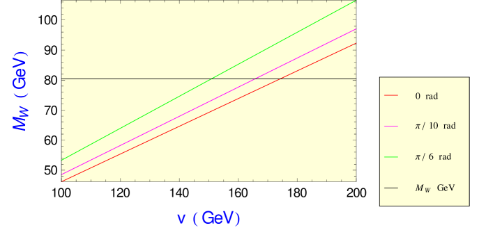
Figure 2: The masses of $W$ to several values of the $\beta$ parameter in therms of the vev of $H_{1}$, the black line means the experimental values of $M_{W}$.

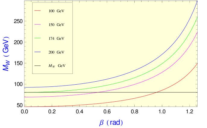
Figure 3: The masses of $W$ in terms of $\beta$ parameter considerating several values of $v_{1}$, again the black line is the experimental value of $M_{W}$.

The neutral massive gauge boson ($Z^{0}$) get the following mass

$$M^{2}_{Z} = \left(\frac{g^{2}+g^{\prime 2}}{4}\right)(v_{1}^{2}+v_{2}^{2})=\frac{g^{2}}{4\cos^{2}\theta_{W}}(v_{1}^{2}+v_{2}^{2})=\frac{M^{2}_{W}}{\cos^{2}\theta_{W}},$$ (87)

where $\theta_{W}$ is the Weinberg angle and it is defined as

$$e=g\sin\theta_{W}=g^{\prime}\cos\theta_{W},$$ (88)

and get a massless foton $A_{m}$. The experimental values are

$$M_{Z} = \left(91.1888\pm 0.0044\right)\,\mbox{\rm GeV},$$

$$\sin^{2}\theta_{W} = 1-\frac{M^{2}_{W}}{M^{2}_{Z}}=0.2320\pm 0.0004,$$ (89)

The rotation in this case is

$$\left(\begin{array}[]{c}A_{m}\\ Z_{m}\end{array}\right)=\left(\begin{array}[]{cc}\sin\theta_{W}&\cos\theta_{W}\\ \cos\theta_{W}&-\sin\theta_{W}\end{array}\right)\left(\begin{array}[]{c}V^{3}_{m}\\ V_{m}\end{array}\right)\,\ ,$$ (96)

it is the exact expression we get in the SM. Therefore the neutral boson gauge sector is exact the same as in the SM.

7.3.1 Photino is not a mass eigenstate

Before we present the neutralinos, we want to discuss first, that we learnt the photon and $Z^{0}$ gauge boson diagonalize the neutral boson sector of the SM, throught the rotation defined at Eq.(96). As we are dealing with supersymmetry, we can ask, are the photino ($\tilde{\gamma}$) and the zino ($\tilde{Z}^{0}$), the superpartnes of photons and $Z^{0}$ gauge boson respectivelly, are masses eigenstates? The answer to this question is no and we will show this results below, this material is a review of the results presented at [37].

In order to show it let us first define their four-component spinors to the photino ($\tilde{\gamma}$) and the zino ($\tilde{Z}$) are

$$\tilde{\gamma}=\left(\begin{array}[]{r}-\imath\lambda_{\gamma}(x)\\ \imath\bar{\lambda}_{\gamma}(x)\end{array}\right)\,\ ,\,\ \tilde{Z}=\left(\begin{array}[]{r}-\imath\lambda_{Z}\\ \imath\bar{\lambda}_{Z}\end{array}\right)\,\ .$$ (101)

By another we can define the winos ($\tilde{W}$) in the following way

$$\tilde{W}(x)\;=\;\left(\begin{array}[]{r}-\imath\lambda^{+}(x)\\ \imath\bar{\lambda}^{-}(x)\end{array}\right)\,\ ,$$ (104)

Where $\lambda^{\pm}$ is defined at Eq.(150), while $\lambda_{\gamma}$ and $\lambda_{Z}$ can be defined as function of $\lambda^{3}$ and $\lambda$ in the following way:

$$\lambda_{\gamma} = \cos\theta_{W}\lambda^{3}-\sin\theta_{W}\lambda,$$

$$\lambda_{Z} = \sin\theta_{W}\lambda^{3}+\cos\theta_{W}\lambda.$$ (105)

$\theta_{W}$ is the Weinberg angle defined at Eq.(88).

The best way to see this result is taking into account Eq.(64) we can write [37]

$$- \frac{1}{2}M\left(\lambda^{1}\lambda^{1}+\lambda^{2}\lambda^{2}+\lambda^{3}\lambda^{3}+\bar{\lambda}^{1}\bar{\lambda}^{1}+\bar{\lambda}^{2}\bar{\lambda}^{2}+\bar{\lambda}^{3}\bar{\lambda}^{3}\right)-\frac{1}{2}M^{\prime}\left(\lambda\lambda+\bar{\lambda}\bar{\lambda}\right)$$ (106)

$$= -M\left(\lambda^{-}\lambda^{+}+\bar{\lambda}^{-}\bar{\lambda}^{+}\right)-\frac{1}{2}\left(M\sin^{2}\theta_{\mbox{w}}+M^{\prime}\cos^{2}\theta_{W}\right)\left(\lambda_{\gamma}\lambda_{\gamma}+\bar{\lambda}_{\gamma}\bar{\lambda}_{\gamma}\right)$$

$$- \frac{1}{2}\left(M\cos^{2}\theta_{W}+M^{\prime}\sin^{2}\theta_{W}\right)\left(\lambda_{Z}\lambda_{Z}+\bar{\lambda}_{Z}\bar{\lambda}_{Z}\right)-\left(M-M^{\prime}\right)\sin({2\theta_{W}})\;\left(\lambda_{\gamma}\lambda_{Z}+\bar{\lambda}_{\gamma}\bar{\lambda}_{Z}\right)$$

$$= -\left\{M_{\tilde{W}}\,\bar{\tilde{W}}\tilde{W}+\frac{1}{2}\left[\,M_{\tilde{\gamma}}\;\bar{\tilde{\gamma}}\tilde{\gamma}+\,M_{\tilde{Z}}\,\bar{\tilde{Z}}\tilde{Z}+\left(M_{\tilde{Z}}-M_{\tilde{\gamma}}\right)\tan({2\theta_{W}})\bar{\tilde{\gamma}}\tilde{Z}\right]\right\}\,\ ,$$

where

$$M_{\tilde{W}} \equiv M,$$

$$M_{\tilde{\gamma}} = M\sin^{2}\theta_{W}+M^{\prime}\cos^{2}\theta_{W}\,\ ,$$

$$M_{\tilde{Z}} = M\cos^{2}\theta_{W}+M^{\prime}\sin^{2}\theta_{W}\,\ .$$ (107)

Therefore a priori the winos are mass eigenstate however the photinos and zino mixing to each other and their mass eigenstates are the neutralinos, see Sec.(7.8). The unification condition give us the following result [34, 35, 36, 37, 104, 105, 106]

$$\frac{M^{\prime}}{M}=\frac{5}{3}\tan^{2}\theta_{W}.$$ (108)

7.4 Higgs Masses

The scalar potential in the MSSM is given by:

$$V^{H}_{MSSM} = (\mu^{2}_{H}+M^{2}_{H_{1}})|H_{1}|^{2}+\frac{1}{8}\left(g^{2}+g^{2}_{Y^{\prime}}\right)(|H_{1}|^{2})^{2}+(\mu^{2}_{H}+M^{2}_{H_{2}})|H_{2}|^{2}+\frac{1}{8}\left(g^{2}+g^{2}_{Y^{\prime}}\right)(|H_{2}|^{2})^{2}$$

$$- \frac{1}{4}\left(g^{2}+g^{2}_{Y^{\prime}}\right)|H_{1}|^{2}|H_{2}|^{2}+\frac{g^{2}}{2}|\bar{H}_{1}H_{2}|^{2}-(M^{2}_{12}\epsilon_{ab}H_{1}^{a}H_{2}^{b}+H.c.).$$

The $8\times 8$ Higgs mass squared matrix breaks up diagonally into three set of $2\times 2$ matrix. After the diagonalization procedure we finish with five physical degrees of freedom form a neutral CP–odd, two neutral CP–even and two charged Higgs bosons denoted by $A^{0}$, $h^{0}$, $H^{0}$, and $H^{\pm}$, respectively [34, 35, 36, 23, 24].

We start our analyses in the CP–odd sector. The mass squared matrix in this sector is found to be

$${\cal M}_{\Im(H^{0})}=\frac{M^{2}_{12}}{v_{1}v_{2}}\left(\begin{array}[]{cc}v_{2}^{2}&v_{1}v_{2}\\ v_{1}v_{2}&v_{1}^{2}\end{array}\right).$$ (110)

We can in a simple way show

$$\det[{\cal M}_{\Im(H^{0})}] = 0,$$

$${\mbox{T}r}[{\cal M}_{\Im(H^{0})}] = \frac{M^{2}_{12}}{v_{1}v_{2}}\left(v_{1}^{2}+v_{2}^{2}\right).$$ (111)

The vanishing determinant and the no vanishing trace of this matrix imply massless (Goldstone boson $G^{0}$) as well as massive neutral model ($A^{0}$). The massive $A^{0}$ particle remains as a pseudoscalar Higgs boson and its mass is proportional to the soft SUSY breaking parameter $M^{2}_{12}$, therefore it should be a heavy than the Higgs boson defined at SM. As in general we suppose all soft parameters are in the TeV range, we can conclude $M_{A}\sim{\cal O}(\mbox{TeV})$.

The mass spectrum in this sector is given by

$$\left(\begin{array}[]{c}G^{0}\\ A^{0}\end{array}\right)=\sqrt{2}\left(\begin{array}[]{cc}\sin\beta&\cos\beta\\ -\cos\beta&\sin\beta\end{array}\right)\left(\begin{array}[]{c}\Im(H_{2}^{0})\\ \Im(H_{1}^{0})\end{array}\right),$$ (112)

and the mass of this sector is given by:

$$M^{2}_{G^{0}} = 0,$$

$$M^{2}_{A^{0}} = \frac{M^{2}_{12}}{v_{1}v_{2}}\left(v^{2}_{1}+v^{2}_{2}\right)=M^{2}_{12}\left(\frac{v_{1}}{v_{2}}+\frac{v_{2}}{v_{1}}\right)=M^{2}_{12}\left(\tan\beta+\cot\beta\right)=M^{2}_{12}\csc\beta\sec\beta,$$

$$M^{2}_{A^{0}} = \frac{2M^{2}_{12}}{\sin(2\beta)}\gg M^{2}_{Z}.$$

$G^{0}$ combines with the massless $Z$ to give their mass, as in the SM. As we want finite mass, the above equation put some constraints in the $\beta$ parameter. It has to satisfy the following constraints

$$\beta\neq 0\,\ \mbox{rad},\,\ \mbox{and}\,\ \beta\neq\frac{\pi}{2}\,\ \mbox{rad}.$$ (114)

$\Re(H)$ denotes the real and $\Im(H)$ the imaginary part of $H$.

On Fig.(15), where we can see this pseudoscalar can be very heavy (as we have discussed above) and as we mentioned above we can see that it diverge when $\beta\rightarrow 0$ rad or when $\beta\rightarrow(\pi/2)$ rad. Of course the minium value of $A$ depend of the value choosen to $M_{12}$ parameter (see the differents colors at Fig.(15)), but we can say its mass can go from $3$ TeV until infinity.

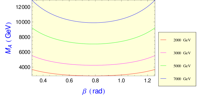
Figure 4: The masses of the pseudoscalar $A$ in terms of the parameter $\beta$, and several values of $M_{12}$.

The charged Higgs sector is very similar to the CP–odd sector. The physical states in terms of the symmetry eigen states are defined in the following way

$$\left(\begin{array}[]{c}H^{\pm}\\ G^{\pm}\end{array}\right)=\left(\begin{array}[]{cc}\sin\beta&-\cos\beta\\ \cos\beta&\sin\beta\end{array}\right)\cdot\left(\begin{array}[]{c}H_{2}^{\pm}\\ (H_{1}^{\mp})^{\dagger}\end{array}\right).$$ (115)

its mass is given by

$$M^{2}_{G^{\pm}} = 0,$$

$$M^{2}_{H^{\pm}} = M^{2}_{W}+M^{2}_{A^{0}}\gg M^{2}_{W}.$$ (116)

$G^{\pm}$ combines with the massless $W^{\pm}$ to give them mass, as in the SM. Remember $M_{W}$ is the gauge $W^{\pm}$ mass, see Eq.(86). On Fig.(5) we see that the mass of the charged Higgs is almost linear in terms of $M_{12}$, as we expected from Eq.(116).

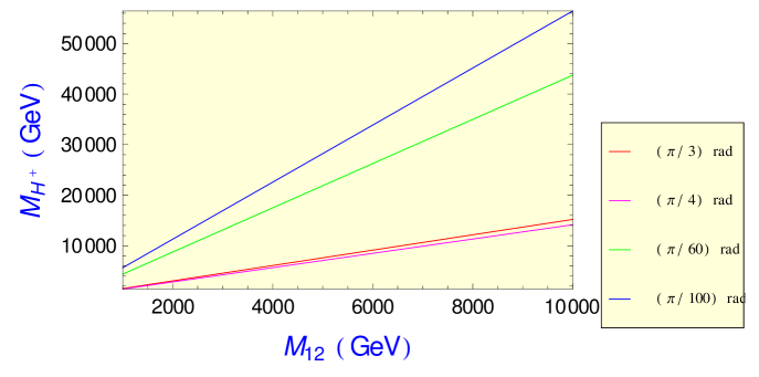
Figure 5: The masses of the charged scalar $H^{+}$ in terms of the $M_{12}$ and several values to the $\beta$ parameter.

The mass squared matrix in the CP–even sector is given by:

$${\cal M}_{\Re(H^{0})}=\left(\begin{array}[]{cc}M^{2}_{A^{0}}\sin^{2}\beta+M^{2}_{Z}\cos^{2}\beta&-(M^{2}_{A^{0}}+M^{2}_{Z})\sin\beta\cos\beta\\ -(M^{2}_{A^{0}}+M^{2}_{Z})\sin\beta\cos\beta&M^{2}_{A^{0}}\cos^{2}\beta+M^{2}_{Z}\sin^{2}\beta\end{array}\right).$$ (117)

Both the determinant as well the trace of this matrix is non vanishing, therefore in this sector we have two massive real scalars. We can in a simple way show

$$\det[{\cal M}_{\Re(H^{0})}] = M^{2}_{A^{0}}M^{2}_{Z}\cos^{2}\left(2\beta\right),$$

$${\mbox{T}r}[{\cal M}_{\Im(H^{0})}] = M^{2}_{A^{0}}+M^{2}_{Z}.$$ (118)

The eigenvalues of this mass matrix are

$$M^{2}_{h^{0},H^{0}}=\frac{1}{2}\left[M^{2}_{A^{0}}+M^{2}_{Z}\mp\sqrt{(M^{2}_{A^{0}}+M^{2}_{Z})^{2}-4M^{2}_{A^{0}}M^{2}_{Z}\cos^{2}(2\beta)}\right].$$ (119)

We note that

$$M^{2}_{h^{0}}+M^{2}_{H^{0}}=M^{2}_{A^{0}}+M^{2}_{Z}.$$ (120)

In equation above we have defined $H$ to be the heavier of the two, it means $M_{h^{0}}<M_{H^{0}}$. The corresponding mass eigenstates are

$$\left(\begin{array}[]{c}h^{0}\\ H^{0}\end{array}\right)=\sqrt{2}\left(\begin{array}[]{cc}\sin\alpha&\cos\alpha\\ -\cos\alpha&\sin\alpha\end{array}\right)\left(\begin{array}[]{c}\Re(H_{2}^{0})-\frac{v_{2}}{\sqrt{2}}\\ \Re(H_{1}^{0})-\frac{v_{1}}{\sqrt{2}}\end{array}\right).$$ (121)

The angle of rotation $\alpha$, defined in the equation above, is seen to obey the followings constraints [34]

$$\sin(2\alpha) = -\frac{M^{2}_{H^{0}}+M^{2}_{h^{0}}}{M^{2}_{H^{0}}-M^{2}_{h^{0}}}\sin(2\beta),$$

$$\cos(2\alpha) = -\frac{M^{2}_{A^{0}}-M^{2}_{Z}}{M^{2}_{H^{0}}-M^{2}_{h^{0}}}\cos(2\beta),$$

$$\tan(2\alpha) = \frac{M^{2}_{H^{0}}+M^{2}_{h^{0}}}{M^{2}_{A^{0}}-M^{2}_{Z}}\tan(2\beta),$$ (122)

considerating Eq.(74) in the first equation above it implies $\sin(2\alpha)<0$ while in the second equation we get $\cos(2\alpha)<0$ . Taking this information we can conclude the range of the new parameter $\alpha$ is given by

$$-\frac{\pi}{2}\leq\alpha\leq 0\,\ (\mbox{rad}).$$ (123)

On Fig(6) we show same if we consider $M_{12}=10$TeV we get $m_{h^{0}}<M_{Z}$. This results is in agreement with the following well known constraints [34, 35, 36]

$$M_{h^{0}}\leq M_{Z}|\cos(2\beta)|,$$ (124)

this implies that $m_{h^{0}}=0$ if $\tan\beta=1$, this results is shown at Fig.(6) where we shown the behaviour of the mass of the ligest scalar as function of $\beta$ parameter. Similar information to the heaviest Higgs is shown in Fig(7). If we consider $M=1000$ GeV we get for several values of $\beta$ parameter masses to all usual scalars of this model, as we can see at Tab.(5).

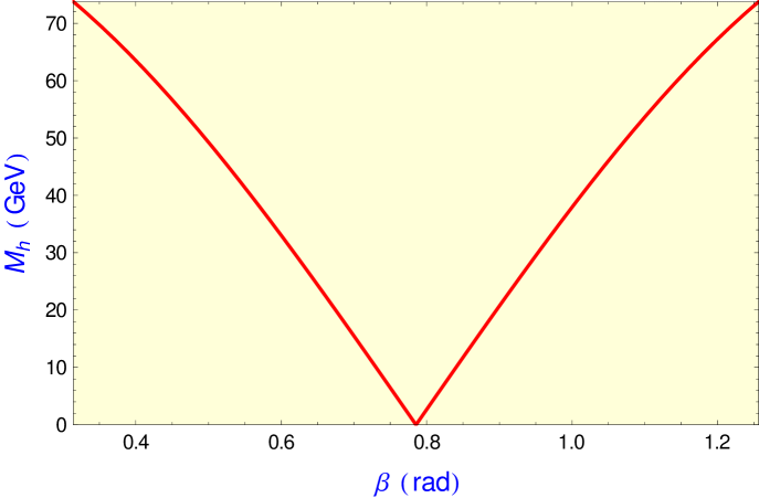
Figure 6: The masses of lighest higgs even scalar $h^{0}$ in terms of the $\beta$ parameter considerating $M_{12}=10000$GeV.

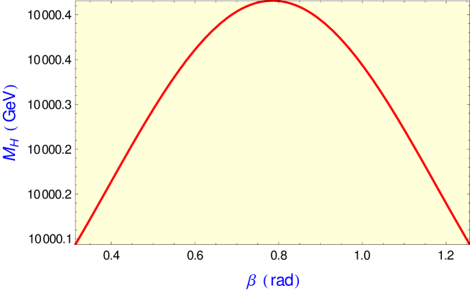
Figure 7: The masses of heaviest higgs Evenn scalar $H^{0}$ in terms of the $\beta$ parameter considerating $M_{12}=1000$GeV.

$\tan\beta$	$m_{A^{0}}(\mbox{GeV})$	$m_{H^{\pm}}(\mbox{GeV})$	$m_{h^{0}}(\mbox{GeV})$	$m_{H^{0}}(\mbox{GeV})$
0.10	3172.85	3173.87	89.35	1000.17
0.20	2266.24	2267.67	83.94	1000.63
0.55	1541.68	1543.78	49.12	1002.95
1.03	1414.52	1416.80	2.65	1004.15
1.56	1483.07	1485.25	37.82	1003.44
2.57	1720.74	1722.61	67.11	1001.90
3.60	1969.70	1971.34	78.05	1001.11
5.80	2443.43	2444.75	85.88	1000.47

Table 5: Masses of all usual scalars to several values of $\tan\beta$.

Therefore, the light scalar $h^{0}$ has a mass smaller than the $Z^{0}$ gauge boson at the tree level. This implies that one has to consider the one-loop corrections which lead to the following result [107]

$$M^{2}_{h^{0}}\simeq M^{2}_{Z}+\frac{3g^{2}M^{4}_{Z}}{16\pi^{2}M^{2}_{W}}\left\{\ln\left(\frac{M^{2}_{\tilde{t}}}{M^{2}_{t}}\right)\left[\frac{2M^{4}_{t}-M^{2}_{t}M^{2}_{Z}}{M^{4}_{Z}}\right]+\frac{M^{2}_{t}}{3M^{2}_{Z}}\right\}.$$ (125)

However, radiative corrections rise it to 130 GeV [53].

We can also write the following ralation [34]:

$$\cos^{2}(\beta-\alpha) = \frac{M^{2}_{h^{0}}(M^{2}_{Z}-M^{2}_{h^{0}})}{M^{2}_{A^{0}}(M^{2}_{H^{0}}-M^{2}_{h^{0}})}.$$ (126)

This equation together with Eq.(119), show that the Higgs sector is completely controlled by two new parameters wchich can be taken to be $M_{A^{0}}$ and $\tan\beta$.

Here we presented only the analyses when CP is conserved. To see the case when CP is not conserved see [108].

7.5 Charged Sleptons Masses

The Lagrangian contains off-diagonal mass terms for the sleptons in the basis $(\tilde{l}_{L},\tilde{l}^{c}_{L}\equiv\tilde{l}_{R})$. So, also here we have to perform a diagonalizing procedure to obtain the physical mass eigenstates, and hence we have

$${\cal L}_{slepton}^{mass} = -\mu f^{l}v_{2}\;\tilde{l}_{L}^{\dagger}\tilde{l}_{R}-\mu f^{l}v_{2}\;\tilde{l}_{R}^{\dagger}\tilde{l}_{L}-f^{l2}v_{1}^{2}\left(\tilde{l}_{L}^{\dagger}\tilde{l}_{L}+\tilde{l}_{R}^{\dagger}\tilde{l}_{R}\right)-M_{L}^{2}\;\tilde{l}_{L}^{\dagger}\tilde{l}_{L}-M_{l}^{2}\;\tilde{l}_{R}^{\dagger}\tilde{l}_{R}$$ (132)

$$= -\left(\begin{array}[]{cc}\tilde{l}_{L}^{\dagger}&\tilde{l}_{R}^{\dagger}\end{array}\right)\left(\begin{array}[]{cc}M_{L}^{2}+f^{l2}v_{1}^{2}&\mu f^{l}v_{2}\\ \mu f^{l}v_{2}&M_{l}^{2}+f^{l2}v_{1}^{2}\end{array}\right)\left(\begin{array}[]{c}\tilde{l}_{L}\\ \tilde{l}_{R}\end{array}\right).$$

By diagonalizing, one obtains the mass eigenstates (in the usual way)

$$\left(\begin{array}[]{c}\tilde{l}_{1}\\ \tilde{l}_{2}\end{array}\right)=\left(\begin{array}[]{cc}\cos{\theta_{\tilde{l}}}&\sin{\theta_{\tilde{l}}}\\ \sin{\theta_{\tilde{l}}}&-\cos{\theta_{\tilde{l}}}\end{array}\right)\left(\begin{array}[]{c}\tilde{l}_{L}\\ \tilde{l}_{R}\end{array}\right),$$ (139)

with

$$\tan{2\theta_{\tilde{l}}} = \frac{2\mu f^{l}v_{2}}{\left(M^{2}_{L}-M^{2}_{l}\right)}=\frac{2\mu m_{l}\tan\beta}{\left(M^{2}_{L}-M^{2}_{l}\right)},$$

and masses respectively given by

$$M_{\tilde{l}_{1},\tilde{l}_{2}}^{2} = m^{2}_{l}+\frac{1}{2}\left[\left(M^{2}_{L}-M^{2}_{l}\right)\pm\sqrt{\left(M^{2}_{L}-M^{2}_{l}\right)^{2}+4\mu^{2}m^{2}_{l}\tan^{2}\beta}\;\right].$$ (140)

For selectrons and smuons, the “left” and “right” states ($\tilde{e}_{L,R}$ and $\tilde{\mu}_{L,R}$) are also the mass eigenstates. For staus, however, the eigenstates are $\tilde{\tau}_{1}$ and $\tilde{\tau}_{2}$. The production of selectrons and sneutrinos were sutied at [34, 35, 74, 76, 109, 110].

Let us now turn to the sneutrinos. In the case of massless neutrinos, there is only one sneutrino, $\tilde{\nu}_{L}$, with a mass

$$m^{2}_{\tilde{\nu}_{L}}=M^{2}_{L}+\frac{M_{Z}^{2}\cos 2\beta}{2},$$ (141)

for each generation. Some Feynman rules to fermion, sfermion and gauge bosons will be presented at 8. The production of selectrons and sneutrinos were sutied at [34, 35, 74, 76, 111].

7.6 Squarks

The squarks $\tilde{q}_{L}$ and $\tilde{q}_{R}$ will mix, in a similar way as happened to the charged sleptons, to more details see [34, 35, 36]. We will donate the physical squark states as $\tilde{q}_{1},\tilde{q}_{2}$, and they are define as

$$\left(\begin{array}[]{c}\tilde{q}_{1}\\ \tilde{q}_{2}\end{array}\right)=\left(\begin{array}[]{cc}\cos{\theta_{\tilde{q}}}&\sin{\theta_{\tilde{q}}}\\ \sin{\theta_{\tilde{q}}}&-\cos{\theta_{\tilde{q}}}\end{array}\right)\left(\begin{array}[]{c}\tilde{q}_{L}\\ \tilde{q}_{R}\end{array}\right).$$ (148)

The Feynman rules to the squarks are presented at [34, 35, 36]. The squark production in nuclear collisions was presented at [34, 35, 74, 76, 112, 113].

The “Snowmass Points and Slopes” (SPS), following [36, 114, 115], are a set of benchmark points and parameter lines in the MSSM parameter space corresponding to different scenarios in the search for Supersymmetry at present and future experiments. There is a very nice review about this convention give at [115]. From this reference we take the Tab.(6). The mass values of squarks and gluinos on these cenarios are shown at Tab.(7).

SPS	Point
mSUGRA:	$m_{0}$	$m_{1/2}$	$A_{0}$	$\tan\beta$
1a	100	250	-100	10
1b	200	400	0	30
2	1450	300	0	10
3	90	400	0	10
4	400	300	0	50
5	150	300	-1000	5
mSUGRA-like:	$m_{0}$	$m_{1/2}$	$A_{0}$	$\tan\beta$	$M_{1}$	$M_{2}=M_{3}$
6	150	300	0	10	480	300
GMSB:	$\Lambda/(10^{3})$	$M_{\rm mes}/(10^{3})$	$N_{\rm mes}$	$\tan\beta$
7	40	80	3	15
8	100	200	1	15
AMSB:	$m_{0}$	$m_{\rm aux}/(10^{3})$		$\tan\beta$
9	450	60		10

Table 6: The parameters for the Snowmass Points and Slopes (SPS). On this table all the scenarios consider $\mbox{sign}\mu=+$ take from [115].

Scenario	$m_{\tilde{g}}\,(GeV)$	$M_{\tilde{q}}\,(GeV)$
SPS1a	595.2	539.9
SPS1b	916.1	836.2
SPS2	784.4	1533.6
SPS3	914.3	818.3
SPS4	721.0	732.2
SPS5	710.3	643.9
SPS6	708.5	641.3
SPS7	926.0	861.3
SPS8	820.5	1081.6
SPS9	1275.2	1219.2

Table 7: Masses of gluinos, squarks, photinos and selectrons in the SPS scenarios [114, 115].

7.7 Charginos Masses

The supersymmetric partners of the $W^{\pm}$ and the $H^{\pm}$ mix to mass eigenstates called charginos $\chi^{\pm}_{i}$ ($i=1,2$) which are four–component Dirac fermions. In order to deduce the properties of the latter we start with the basis [104]

$$\psi^{+}=\left(-\imath\lambda^{+}\!,\,\tilde{H}^{+}_{2}\right)^{T},\hskip 17.07164pt\psi^{-}=\left(-\imath\lambda^{-}\!,\,\tilde{H}^{-}_{1}\right)^{T},$$ (149)

where

$$\lambda^{\pm}=\frac{1}{\sqrt{2}}\,(\lambda^{1}\mp\imath\lambda^{2}),$$ (150)

see definition of $W$ boson given at Eq.(85). The mass terms of the lagrangian of the charged gaugino–higgsino system can then be written as

$${\cal L}_{m}=-\frac{1}{2}\,\left((\psi^{+})^{T}\!,\,(\psi^{-})^{T}\right)\,\,Y^{\pm}\,\left(\begin{array}[]{c}\psi^{+}\\ \psi^{-}\end{array}\right)+hc$$ (151)

where

$$Y^{\pm}=\left(\begin{array}[]{cc}0&X^{T}\\ X&0\end{array}\right),$$ (152)

with

$$X=\left(\begin{array}[]{cc}M&\sqrt{2}\,M_{W}\sin\beta\\ \sqrt{2}\,M_{W}\cos\beta&\mu\end{array}\right).$$ (153)

Its matrix has

$$\det[X] = \det[X^{T}]=\mu M-2M^{2}_{W}\sin\beta\cos\beta=\mu M-M^{2}_{W}\sin\left(2\beta\right),$$

$${\mbox{T}r}[X] = {\mbox{T}r}[X^{T}]=\mu+M.$$ (154)

The matrix $Y^{\pm}$ in Eq.(152) satisfy the following relation

$$\det(Y^{\pm}-\lambda I)=\det\left[\left(\begin{array}[]{cc}-\lambda&X^{T}\\ X&-\lambda\end{array}\right)\right]=\det(\lambda^{2}-X^{T}\cdot X),$$ (157)

so we only have to calculate $X^{t}\cdot X$ to obtain the eigenvalues.

From Eq.(153) we can write

$$X\cdot X^{T} = \left(\begin{array}[]{cc}M^{2}+2M^{2}_{W}\sin^{2}\beta&\sqrt{2}M_{W}\left(M\cos\beta+\mu\sin\beta\right)\\ \sqrt{2}M_{W}\left(M\cos\beta+\mu\sin\beta\right)&\mu^{2}+2M^{2}_{W}\cos^{2}\beta\end{array}\right),$$ (160)

$$X^{T}\cdot X = \left(\begin{array}[]{cc}M^{2}+2M^{2}_{W}\cos^{2}\beta&\sqrt{2}M_{W}\left(M\sin\beta+\mu\cos\beta\right)\\ \sqrt{2}M_{W}\left(M\sin\beta+\mu\cos\beta\right)&\mu^{2}+2M^{2}_{W}\sin^{2}\beta\end{array}\right).$$ (163)

Therefore $X\cdot X^{T}\neq X^{T}\cdot X$, however we can show the folowings results

$$\det[X\cdot X^{T}] = \det[X^{T}\cdot X]=\left[\mu M-M^{2}_{W}\sin\left(2\beta\right)\right]^{2},$$

$${\mbox{T}r}[X\cdot X^{T}] = {\mbox{T}r}[X^{T}\cdot X]=\mu^{2}+M^{2}+2M^{2}_{W}.$$ (164)

Since $X^{T}\cdot X$ is a symmetric matrix, $\lambda^{2}$ must be real, and positive because $Y^{\pm}$ is also symmetric.

The mass matrix $X$ is diagonalized by two $2\!\times\!2$ unitary matrices $U$ and $V$:

$${\cal M}^{\mbox{diag}}_{C}=U^{*}X\,V^{-1}.$$ (165)

We can see this result from the following

$$\left(\psi^{-}\right)^{T}X\psi^{+} = \left(U^{-1}U\psi^{-}\right)^{T}XV^{-1}V\psi^{+}=\left(\psi^{-}\right)^{T}U^{t}U^{*}XV^{-1}V\psi^{+}$$ (166)

$$= \left(\tilde{\chi}^{-}\right)^{t}{\cal M}^{\mbox{diag}}_{C}\tilde{\chi}^{+}.$$

In the last equality we have defined, $U$ and $V$ are the unitary matrices, the following rotations

$$\chi^{+}_{i} = V_{ij}\,\psi^{+}_{j},$$

$$\chi^{-}_{i} = U_{ij}\,\psi^{-}_{j},\hskip 17.07164pti,j=1,2,$$ (167)

with

$${\cal M}^{\mbox{diag}}_{C}=\mbox{diag}\left(m_{\chi_{1}},m_{\chi_{2}}\right).$$ (168)

with real nonnegative entries. From Eq.(165) we see that

$$\left({\cal M}^{\mbox{diag}}_{C}\right)^{2}=V\left(X^{T}\cdot X\right)V^{-1}=U^{*}\left(X\cdot X^{T}\right)\left(U^{*}\right)^{-1},$$ (169)

therefore $U$ and $V$ diagonalize the hermitian matrices $X\cdot X^{T}$ and $X^{T}\cdot X$.

Moreover, assuming CP conservation, the CP violate case is presented at [116], we choose a phase convention in which $U$ and $V$ are real. The eigenvalues of Eq.(153) is given by ($i=1,2$)

$$m^{2}_{\chi_{i}} = \frac{1}{2}\,\left[|M^{2}|+|\mu^{2}|+2M_{W}^{2}\right.$$ (170)

$$\pm \left.\sqrt{(|M^{2}|-|\mu^{2}|)^{2}+4M^{4}_{W}\cos^{2}(2\beta)+4M^{2}_{W}\left[|M^{2}|+|\mu^{2}|+2\Re(M\mu)\sin(2\beta)\right]}\right].$$

The mass eigenstates in Dirac notation are given by

$$\tilde{\chi}^{+}_{i}=\left(\begin{array}[]{c}\chi^{+}_{i}\\ \overline{\chi^{-}_{i}}\end{array}\right),\hskip 17.07164pti,j=1,2.$$ (171)

We take $\tilde{\chi}^{+}_{1}$ to be the lighter chargino per definition. The charginos, like all the charged fermions in the SM, are Dirac fermions [79].

If we consider $\mu=100$ GeV and $M=1000$ GeV we get for several values of $\beta$ parameter masses to the lighest charginos of ${\cal O}(M_{Z})$ while the heaviest charginos has masses around TeV region, as we can see at Tab.(8). On Fig.(8) we have fixed $M$ and we have considered several values to the $\mu$ parameter. On Fig.(9) we have fixed $\beta$ and we have considered several values to the $\mu$ parameter. On Fig.(10) we have fixed $\beta$ and we have considered several values to the $M$ parameter. We see from all this figure that in media the average mass to the lighest charginos is around 100 GeV. Tḧe couplings of charginos are presented at [34, 35, 36, 104]. The productions of charginos was studied at [34, 35, 36, 74, 76, 98, 104].

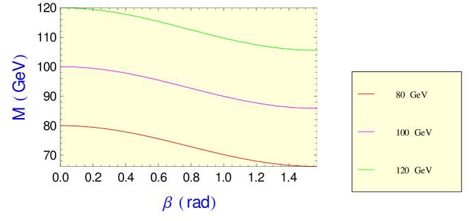
Figure 8: The masses of lighest chargino in terms of the $\beta$ parameter considerating $M=1000$ GeV and several values of $\mu$ parameter.

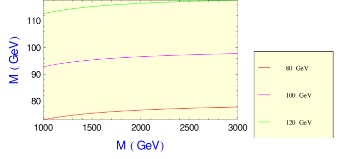
Figure 9: The masses of lighest chargino in terms of the $M$ parameter considerating $\beta=(\pi/4)$ rad and several values of $\mu$ parameter.

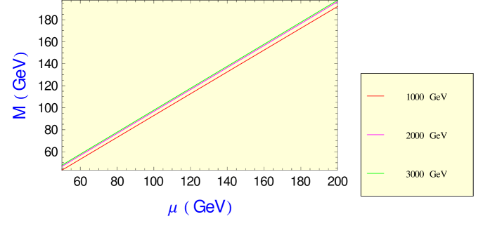
Figure 10: The masses of lighest chargino in terms of the $\mu$ parameter.

7.8 Neutralinos Masses

The neutral gauginos, see Sec.(7.3.1), and neutral higgsinos also mix and these new state is known as neutralinos [34, 35, 36, 37, 105, 106]. Their mass eigenstates are the neutralinos. In this review we choose the basis [37, 105, 106]

$$\psi^{0}_{MSSM}=\left(\begin{array}[]{cccc}\imath\lambda_{\gamma}&\imath\lambda_{Z}&\tilde{H}^{0}_{1}&\tilde{H}^{0}_{2}\end{array}\right)^{\!\rm T}.\hskip 17.07164pt$$ (172)

The mass terms of the neutral gaugino–higgsino system can then be written as

$${\cal L}_{m}=-\frac{1}{2}\,(\psi^{0})^{\rm T}_{MSSM}\,Y^{neutralino}_{MSSMRPC}\,\psi^{0}_{MSSM}+\,\ hc$$ (173)

with

$$Y^{neutralino}_{MSSMRPC}=\left(\begin{array}[]{cccc}M_{\tilde{\gamma}}&\frac{1}{4}\left(M_{\tilde{Z}}-M_{\tilde{\gamma}}\right)\tan({2\theta_{W}})&0&0\\ \frac{1}{4}\left(M_{\tilde{Z}}-M_{\tilde{\gamma}}\right)\tan({2\theta_{W}})&M_{\tilde{Z}}&M_{Z}\sin\beta&-M_{Z}\cos\beta\\ 0&M_{Z}\sin\beta&0&-\mu\\ 0&-M_{Z}\cos\beta&-\mu&0\end{array}\right)\,\ .$$ (174)

Its matrix has

$$\det[Y] = \mu^{2}\left\{\left[\left(\frac{M_{\tilde{Z}}-M_{\tilde{\gamma}}}{4}\right)\tan(2\theta_{W})\right]^{2}-M_{\tilde{\gamma}}M_{\tilde{Z}}\right\}+M^{2}_{Z}M_{\tilde{\gamma}}\mu\sin(2\beta)$$

$$= -MM^{\prime}\mu^{2}+M^{2}_{Z}\mu\left(M\sin^{2}\theta_{W}-M^{\prime}\cos^{2}\theta_{W}\right)\sin\left(2\beta\right)+\frac{M^{4}_{Z}}{4}\sin\left(2\theta_{W}\right)\sin\left(2\beta\right),$$

$${\mbox{T}r}[Y] = M_{\tilde{\gamma}}+M_{\tilde{Z}}=M+M^{\prime}.$$ (175)

We wrote the matrix in the basis os photino and zino. However, it is more used it, on the basis of $\lambda_{3}$ and $\lambda$, on this base the matrix is given at [34, 35].

The mass matrix $Y$ is diagonalized by a $4\!\times\!4$ unitary matrix $N$,

$$N^{*}\,Y\,N^{-1}={\cal M}_{N}$$ (176)

with ${\cal M}_{N}$ the diagonal mass matrix. The eigenvalues ${\cal M}_{N}$ and the matrix $N$ in general are obtained numerically. However if all parameter in the matrix $Y$ are real, an analytical calculation to eigenstates and eigenvectors are possible [106].

The mass eigenstates in two–component notation then are

$$\chi^{0}_{i}=N_{ij}\,\psi^{0}_{j},\hskip 17.07164pti,j=1\ldots 4,$$ (177)

and we can find them in the following way

$$\left(\begin{array}[]{c}\chi^{0}_{1}\\ \chi^{0}_{2}\\ \chi^{0}_{3}\\ \chi^{0}_{4}\end{array}\right)=\left(\begin{array}[]{cccc}\eta_{1}&0&0&0\\ 0&\eta_{2}&0&0\\ 0&0&\eta_{3}&0\\ 0&0&0&\eta_{4}\end{array}\right)\left(N\right)\left(\begin{array}[]{c}\imath\lambda_{\gamma}\\ \imath\lambda_{Z}\\ \tilde{H}_{1}^{0}\\ \tilde{H}_{2}^{0}\end{array}\right)$$ (178)

The four-by-four matrix $N$ diagonalizes the symmetric mass matrix ${\cal M}_{N}$ of the neutral Weyl spinors, see Eq.(253), where the eigenvalues are arranged such that $|m_{\chi^{0}_{1}}|<|m_{\chi^{0}_{2}}|<|m_{\chi^{0}_{3}}|<|m_{\chi^{0}_{4}}|$. The parameter $\eta_{i}$ is introduced in order to change the phase of the particle whose eigenvalue becomes negative, it means it is defined as follow

$$\eta_{i}=\left\{\begin{array}[]{c}1,m_{\chi^{0}_{i}}>0,\\ \imath,m_{\chi^{0}_{i}}<0,\end{array}\right.,\,\ i=1,\ldots 4,$$ (179)

and

$$m_{\chi^{0}_{i}}=\eta^{2}_{i}m_{\chi^{0}_{i}}.$$ (180)

The four–component notation to the neutralinos is given as

$$\tilde{\chi}^{0}_{i}=\left(\begin{array}[]{c}\chi^{0}_{i}\\ \overline{\chi^{0}_{i}}\end{array}\right),\hskip 17.07164pti=1\ldots 4.$$ (181)

On Fig.(11) we have fixed $M$ and we have considered several values to the $\mu$ parameter. We see that the mass of the lighest neutralino is around 100 GeV. If we consider $\mu=100$ GeV and $M=M^{\prime}=1000$ GeV we get for several values of $\beta$ parameter masses to the lighest charginos of ${\cal O}(M_{Z})$ while the heaviest charginos has masses around TeV region, as we can see at Tab.(8).

$\tan\beta$	$m_{\tilde{\chi}^{\pm}_{1}}(\mbox{GeV})$	$m_{\tilde{\chi}^{\pm}_{2}}(\mbox{GeV})$	$m_{\tilde{\chi}^{0}_{1}}(\mbox{GeV})$	$m_{\tilde{\chi}^{0}_{2}}(\mbox{GeV})$	$m_{\tilde{\chi}^{0}_{3}}(\mbox{GeV})$	$m_{\tilde{\chi}^{0}_{4}}(\mbox{GeV})$
0.00	100	1000	95.51	103.84	1000.00	1008.33
0.10	99.86	1000.14	96.03	104.27	1000.06	1008.18
0.20	99.43	1000.57	96.53	104.68	1000.22	1007.93
0.55	96.71	1003.29	97.68	105.63	1001.20	1006.74
1.03	92.67	1007.33	98.08	105.95	1001.92	1005.95
1.56	89.95	1010.05	97.85	105.77	1001.47	1006.45
2.57	87.70	1012.30	97.26	105.28	1000.71	1007.30
3.60	86.87	1013.13	96.86	104.95	1000.40	1007.69
5.80	86.27	1013.73	96.39	104.56	1000.16	1008.01

Table 8: Masses of charginos and neutralinos to several values of $\tan\beta$.

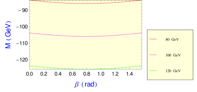
Figure 11: The masses of lighest neutralino in terms of the $\beta$ parameter considerating $M=M^{\prime}=1000$ GeV and several values to $\mu$ parameter.

Tḧe couplings of neutralinos are presented at [34, 35, 36, 37, 105] and the productions of neutralinos as well its decays channel was studied at [34, 35, 36, 74, 76, 98, 99, 105]. We have presented only the analyses when we respect CP invariance. The calaculation of mass spectrum in the case of CP violation can be found at [35]. We want to finish this section saying that the chargino and neutralino mixing pattern are complex. This subject is discussed at [34, 35].

8 Some Feynman Rules to fermions in the MSSM.

We can take these interactions terms from ${\cal L}_{Quarks}$ and ${\cal L}_{Leptons}$. The interaction between fermion-fermion with the gauge bosons, see Eqs.(19), came from

$${\cal L}_{ffV} = \frac{g}{2}(\bar{Q}\bar{\sigma}^{m}\sigma^{i}Q+\bar{L}\bar{\sigma}^{m}\sigma^{i}L)V^{i}_{m}+\frac{g^{\prime}}{2}\left(Y_{Q}\bar{Q}\bar{\sigma}^{m}Q+Y_{L}\bar{L}\bar{\sigma}^{m}L\right.$$ (182)

$$+ \left.Y_{u^{c}}\overline{u^{c}}\bar{\sigma}^{m}u^{c}+\frac{g^{\prime}}{2}Y_{d^{c}}\overline{d^{c}}\bar{\sigma}^{m}d^{c}+\frac{g^{\prime}}{2}Y_{l^{c}}\overline{l^{c}}\bar{\sigma}^{m}l^{c}\right)V^{\prime}_{m}$$

$$= {\cal L}^{charged}_{ffV}+{\cal L}^{neutral}_{ffV},$$

while the interaction sfermion-sfermion with the gauge boson is get from

$${\cal L}_{\tilde{l}\tilde{l}V} = \frac{\imath g}{2}\left(\bar{\tilde{Q}}\sigma^{i}\partial^{m}\tilde{Q}-\tilde{Q}\sigma^{i}\partial^{m}\bar{\tilde{Q}}+\bar{\tilde{L}}\sigma^{i}\partial^{m}\tilde{L}-\tilde{L}\sigma^{i}\partial^{m}\bar{\tilde{L}}\right)V^{i}_{m}$$ (183)

$$+ \frac{ig^{\prime}}{2}\left[Y_{Q}\left(\bar{\tilde{Q}}\partial^{m}\tilde{Q}-\tilde{Q}\partial^{m}\bar{\tilde{Q}}\right)+Y_{L}\left(\bar{\tilde{L}}\partial^{m}\tilde{L}-\tilde{L}\partial^{m}\bar{\tilde{L}}\right)+Y_{u^{c}}\left(\overline{\tilde{u}^{c}}\partial^{m}\tilde{u}^{c}-\tilde{u}^{c}\partial^{m}\overline{\tilde{u}^{c}}\right)\right.$$

$$+ \left.Y_{d^{c}}\left(\overline{\tilde{d}^{c}}\partial^{m}\tilde{d}^{c}-\tilde{d}^{c}\partial^{m}\overline{\tilde{d}^{c}}\right)+Y_{l^{c}}\left(\overline{\tilde{l}^{c}}\partial^{m}\tilde{l}^{c}-\tilde{l}^{c}\partial^{m}\overline{\tilde{l}^{c}}\right)\right]V^{\prime}_{m}$$

$$= {\cal L}^{charged}_{\tilde{f}\tilde{f}V}+{\cal L}^{neutral}_{\tilde{f}\tilde{f}V},$$

after doing some simple mathematical manipulation we arrive in the following Feynman rules see Eqs.(85,139,148), for charged currents [34, 35, 36]

$${\cal L}^{charged}_{ffV} = \frac{-g}{\sqrt{2}}\left[\left(\bar{u}\gamma^{m}d_{L}+\bar{\nu}\gamma^{m}e_{L}\right)W^{+}_{m}+\left(\bar{d}\gamma^{m}u_{L}+\bar{e}\gamma^{m}\nu_{L}\right)W^{-}_{m}\right],$$

$${\cal L}^{charged}_{\tilde{f}\tilde{f}V} = \frac{-\imath g}{\sqrt{2}}\left[\left(\tilde{u}^{\star}_{L}\stackrel{{\scriptstyle\leftrightarrow}}{{\partial}}^{m}\tilde{d}_{L}+\tilde{\nu}^{\star}_{L}\stackrel{{\scriptstyle\leftrightarrow}}{{\partial}}^{m}\tilde{e}_{L}\right)W^{+}_{m}+\left(\tilde{d}^{\star}_{L}\stackrel{{\scriptstyle\leftrightarrow}}{{\partial}}^{m}\tilde{u}_{L}+\tilde{e}^{\star}_{L}\stackrel{{\scriptstyle\leftrightarrow}}{{\partial}}^{m}\tilde{\nu}_{L}\right)W^{-}_{m}\right],$$

the chiral Dirac matrix $\gamma_{5}$ is defined as [16]

$$\gamma^{5}\equiv\left(\begin{array}[]{cc}1&0\\ 0&-1\end{array}\right)\,\ ,$$ (185)

so the right-handed projector ($R$) and left-handed projector ($L$) are given as

$$R = \frac{1}{2}\left(1+\gamma^{5}\right)=\left(\begin{array}[]{cc}1&0\\ 0&0\end{array}\right)\,\ .$$ (188)

$$L = \frac{1}{2}\left(1-\gamma^{5}\right)=\left(\begin{array}[]{cc}0&0\\ 0&1\end{array}\right)\,\ ,$$ (191)

and as usual, we have

$$f_{L}\equiv Lf,\,\ f_{R}\equiv Rf.$$ (192)

where we have defined

$$\bar{\phi}\stackrel{{\scriptstyle\leftrightarrow}}{{\partial}}\Phi\equiv\bar{\phi}\left(\partial\Phi\right)-\left(\partial\bar{\phi}\right)\Phi,$$ (193)

while the Feynman Rules for neutral currents see Eqs.(96,139,148) [34, 35, 36]

$${\cal L}^{neutral}_{ffV} = \frac{-g}{\cos\theta_{W}}\sum_{f}\bar{f}\left[\left(T_{3f}-\sin^{2}\theta_{W}Q_{f}\right)L-\sin^{2}\theta_{W}Q_{f}R\right]fZ_{m}-e\sum_{f}\bar{f}\gamma^{m}fA_{m},$$

$${\cal L}^{neutral}_{\tilde{f}\tilde{f}V} = \frac{-\imath g}{\cos\theta_{W}}\sum_{f}\left[\tilde{f}^{\star}_{L}\stackrel{{\scriptstyle\leftrightarrow}}{{\partial}}^{m}\left(T_{3f}-\sin^{2}\theta_{W}Q_{f}\right)\tilde{f}_{L}-\tilde{f}^{\star}_{R}\stackrel{{\scriptstyle\leftrightarrow}}{{\partial}}^{m}\left(\sin^{2}\theta_{W}Q_{f}\right)\tilde{f}_{R}\right]Z_{m}$$ (194)

$$- \imath e\sum_{f}Q_{f}\left(\tilde{f}^{\star}_{L}\stackrel{{\scriptstyle\leftrightarrow}}{{\partial}}^{m}\tilde{f}_{L}+\tilde{f}^{\star}_{R}\stackrel{{\scriptstyle\leftrightarrow}}{{\partial}}^{m}\tilde{f}_{R}\right)A_{m},$$

the summation $f$ is taken over the fermion species.

The Feynman Rules to the coupling Fermion-Fermion-Higgs, for the usual scalars see Eqs.(112,115,121) [34, 35, 36]

$${\cal L}_{ffH} = -f^{u}\epsilon_{ij}\left(H^{i}_{2}Q^{j}u^{c}+h.c.\right)-f^{d}\epsilon_{ij}\left(H^{i}_{1}Q^{j}d^{c}+h.c.\right)-f^{l}\epsilon_{ij}\left(H^{i}_{1}L^{j}l^{c}+h.c.\right),$$ (195)

using the physical fields we get

$${\cal L}_{ffH^{0}_{i}} = \frac{-gm_{u}}{2M_{W}\sin\beta}\left(\cos\alpha\bar{u}uh^{0}-\sin\alpha\bar{u}uH^{0}-\imath\cos\beta\bar{u}\gamma^{5}uA^{0}\right)$$ (196)

$$- \frac{gm_{d}}{2M_{W}\cos\beta}\left(\sin\alpha\bar{d}dh^{0}+\cos\alpha\bar{d}dH^{0}-\imath\sin\alpha\bar{d}\gamma^{5}dA^{0}\right)$$

$$- \frac{gm_{e}}{2M_{W}\cos\beta}\left(\sin\alpha\bar{e}eh^{0}+\cos\alpha\bar{e}eH^{0}-\imath\sin\beta\bar{e}\gamma^{5}eA^{0}\right)$$

$$+ \frac{g}{2\sqrt{2}M_{W}}\left[\left(m_{u}\cot\beta+m_{d}\tan\beta\right)\bar{u}d+\left(m_{d}\tan\beta-m_{u}\cot\beta\right)\bar{u}\gamma^{5}d\right.$$

$$+ \left.m_{e}\tan\beta\bar{\nu}_{e}\left(1+\gamma^{5}\right)e\right]H^{+},$$

where to the usual scalar see Tab.(5).

9 The Next to Minimal Supersymmetric Standard Model (NMSSM).

It is possible to extend the Higgs sector in such way that the $SU(3)_{C}\otimes SU(2)_{L}\otimes U(1)_{Y}$ gauge symmetry is spontaneously broken at tree level, even in the supersymmetric limit. The simplest extension is to include a complex scalar field wchich is an $SU(3)_{C}\otimes SU(2)_{L}\otimes U(1)_{Y}$ gauge singlet, this model is known as the Next to Minimal Supersymmetric Standard Model (NMSSM) [10, 11, 34, 64, 65] .

The NMSSM is characterized by the following new singlet superfieldfield

$$\hat{S}\sim({\bf 1},{\bf 1},0),$$ (197)

again the the numbers in parenthesis refers to the $(SU(3)_{C},SU(2)_{L},U(1)_{Y}$) quantum numbers. This new superfield is introduced in the following chiral superfield [16, 34, 64]

$$\hat{S}(y,\theta) = S(y)+\sqrt{2}\theta\tilde{S}(y)+\theta\theta F_{S}(y),$$ (198)

and $S$ is the scalar field and its vacuum expectation value (vev) is given by

$$\langle S\rangle\equiv\frac{x}{\sqrt{2}}.$$ (199)

The fermionic field $\tilde{S}$, defined at Eq.(198), is known as singlino. Due the fact we introduce this new superfield, we get as consequence that the mass bounds for the Higgs bosons and neutralinos are weakened as we want to show next. The goal of this review is to present both sector in this kind of model in details, the main motivation to study this kind of model can be found at [10, 11].

The supersymetric Lagrangian of the NMSSM is given by

$${\cal L}^{NMSSM}_{SUSY}={\cal L}^{chiral}_{SUSY}+{\cal L}^{Gauge}_{SUSY}.$$ (200)

The Lagrangian defined in the equation (200) contains the lagrangian ${\cal L}_{quarks}$ and ${\cal L}_{leptons}$, and these terms are the same as presented at MSSM see Eqs.(39).

In this model, We need to modify only ${\cal L}_{Higgs}$, and we get

$${\cal L}_{Higgs} = \int d^{4}\theta\;\left[\,K\left(\hat{\bar{H}}_{1}e^{2g\hat{V}+g^{\prime}\left(-\frac{1}{2}\right)\hat{V}^{\prime}},\hat{H}_{1}\right)+K\left(\hat{\bar{H}}_{2}e^{2g\hat{V}+g^{\prime}\left(\frac{1}{2}\right)\hat{V}^{\prime}},\hat{H}_{2}\right)+K\left(\hat{\bar{S}},\hat{S}\right)\right].$$ (201)

The terms $\left({\cal D}_{m}H_{1}\right)$ and $\left({\cal D}_{m}H_{2}\right)$ give the mass to the gauge bosons $W^{\pm}$ and $Z^{0}$ in the same way as happen in the MSSM, see Eq.(83).

The most general superpotential of NMSSM is defined as

$$W_{NMSSM} = W^{MSSM}_{3RC}+\lambda\left(\hat{H}_{1}\hat{H}_{2}\right)\hat{S}-\frac{\kappa}{3}\left(\hat{S}\right)^{3}.$$ (202)

where $W^{MSSM}_{3RC}$ is given by Eq.(42).

In this case, the parameter $\mu$ of the MSSM is generated as

$$\mu\equiv\lambda\frac{x}{\sqrt{2}}.$$ (203)

and $x$ is expected to be ${\cal O}(v_{1},v_{2})$ in most theories. Since $\lambda$ is also in the perturbative domain, we have a natural explanation for keeping $\mu\ll M_{Pl}$, given that $v_{1},v_{2}\ll M_{Pl}$.

We want to stress that this superpotential has no bilinear terms, remember they lead to naturalness problems and, furthermore, do not appear in a large class of superstring models [2, 64, 65]. The sign of $\kappa$ coupling has been chosen for later convenience.

We can add the following soft supersymmetry breaking terms to the NMSSM

$${\cal L}^{NMSSM}_{Soft} = {\cal L}^{MSSM}_{SMT}+{\cal L}^{MSSM}_{GMT}+{\cal L}^{NMSSM}_{INT}\,\ ,$$ (204)

where ${\cal L}^{MSSM}_{SMT}$ and ${\cal L}^{MSSM}_{GMT}$ are introduced at Eqs.(63,64), respectively. There is an interaction term ${\cal L}^{NMSSM}_{INT}$ of the form [2, 64, 65]

$${\cal L}^{NMSSM}_{INT} = {\cal L}^{MSSM}_{INT}+\left(\lambda A_{\lambda}H_{1}H_{2}S+\frac{\kappa A_{\kappa}}{3}S^{3}+h.c.\right)\,\ .$$ (205)

The term ${\cal L}^{MSSM}_{INT}$ is given at Eq.(65), in this model the first term at this equation is absent.

The soft Supersymmetry breaking terms are given by

$$V_{soft}^{NMSSM} = \tilde{m}_{1}^{2}|H_{1}|^{2}+\tilde{m}_{2}^{2}|H_{2}|^{2}+\tilde{m}_{s}^{2}|S|^{2}-\left[\lambda A_{\lambda}\left(\epsilon_{\alpha\beta}H_{1}^{\alpha}H_{2}^{\beta}\right)S+\frac{\left(\kappa A_{\kappa}\right)}{3}\left(S\right)^{3}+h.c.\right].$$ (206)

In the presence of soft supersymmetry breaking, one would expect

$$x={\cal O}(|m_{i}|)={\cal O}(M_{W}),$$ (207)

and hence $\mu={\cal O}(M_{W})\ll M_{Pl}$.

10 Scalar Potential at NMSSM

We assume that squarks and sleptons fields have zero vaccum expectation value (VEVEs). After the scalar fields $H_{1}$,$H_{2}$ and $S$ develop their VEVs $v_{1}$, $v_{2}$ and $x$, respectively, they can be expanded in the usual way as

$$H_{1}=\left(\begin{array}[]{c}\frac{1}{\sqrt{2}}\left(v_{1}+\phi_{1}+\imath\varphi_{1}\right)\\ H_{1}^{-}\end{array}\right),\,\ H_{2}=\left(\begin{array}[]{c}H_{2}^{+}\\ \frac{1}{\sqrt{2}}\left(v_{2}+\phi_{2}+\imath\varphi_{2}\right)\end{array}\right),\,\ S=\frac{1}{\sqrt{2}}\left(x+\sigma+\imath\xi\right)\,.$$ (212)

The scalar potential, as usual in supersymmetric models, is written as

$$V^{NMSSM} = M_{H_{1}}^{2}|H_{1}|^{2}+M_{H_{2}}^{2}|H_{2}|^{2}+M_{S}^{2}|S|^{2}-\left[\lambda A_{\lambda}\left(\epsilon_{\alpha\beta}H_{1}^{\alpha}H_{2}^{\beta}\right)S+\frac{\left(\kappa A_{\kappa}\right)}{3}\left(S\right)^{3}+h.c.\right]$$ (213)

$$+ \left(|H_{1}|^{2}+|H_{2}|^{2}\right)\left|\lambda S\right|^{2}+\left|\lambda\left(H_{1}H_{2}\right)S+\kappa S^{2}\right|^{2}$$

$$+ \frac{g^{2}}{8}\left(\bar{H}_{1}\sigma^{i}H_{1}+\bar{H}_{2}\sigma^{i}H_{2}\right)^{2}+\frac{g^{\prime 2}}{8}\left(\bar{H}_{1}H_{1}-\bar{H}_{2}H_{2}\right)^{2}.$$

$\lambda$, $\kappa$, $A_{\lambda}$ and $A_{\kappa}$ can be complex number.

There are various limiting cases in wchich the scalar Higgs masses and mixing angles can be evaluated perturbatively

1. $x\gg v_{1},v_{2}$ with $\lambda$ and $\kappa$ fixed;

2. $x\gg v_{1},v_{2}$ with $\lambda x$ and $\kappa x$ fixed;

in the last limit the MSSM with two Higgs doublets and no Higgs singlets is obtained [65].

10.1 Constraints

We can use the minimization condition to re-express the soft supersymmetry breaking terms $M_{H_{1}}^{2}$, $M_{H_{2}}^{2}$ and $M_{S}^{2}$ in terms of the vevs and of the remaind parameters $\lambda$, $\kappa$, $A_{\lambda}$ and $A_{\kappa}$

$$M_{H_{1}}^{2} = \lambda A_{\lambda}\frac{v_{2}x}{v_{1}}-\lambda^{2}\left(x^{2}+v_{2}^{2}\right)+\lambda\kappa\frac{v_{2}x^{2}}{v_{1}}+\left(\frac{g^{2}+g^{\prime 2}}{4}\right)\left(v_{2}^{2}-v_{1}^{2}\right),$$ (214)

$$M_{H_{2}}^{2} = \lambda A_{\lambda}\frac{v_{1}x}{v_{2}}-\lambda^{2}\left(x^{2}+v_{1}^{2}\right)+\lambda\kappa\frac{v_{1}x^{2}}{v_{2}}+\left(\frac{g^{2}+g^{\prime 2}}{4}\right)\left(v_{1}^{2}-v_{2}^{2}\right),$$ (215)

$$M_{S}^{2} = \lambda A_{\lambda}\frac{v_{1}v_{2}}{x}+\kappa A_{\kappa}x-\lambda^{2}\left(v_{1}^{2}+v_{2}^{2}\right)-2\kappa^{2}x^{2}+2\lambda\kappa v_{1}v_{2}.$$ (216)

Therefore, the mass terms for the Higgs fields, can be expressed in terms of the six parameters $\lambda$, $\kappa$, $A_{\lambda}$, $A_{\kappa}$, $x$ and $\tan\beta$.

10.2 Charged Higgs

In the Charged Higgs sector we get an unphysical Goldstone boson and the physical charged Higgs field defined at Eq.(115) and therefore the mass eigenvector are the same in those models MSSM and NMSSM.

The mass squared matrix in this sector is found to be

$$\left({\cal M}^{NMSSM}_{H^{\pm}}\right)^{2}=\left[\frac{v_{1}v_{2}}{2}(g-2\lambda^{2})+\frac{\lambda x}{g}(\kappa x+A_{\lambda})\right]{\cal M}^{2}_{H^{\pm}},$$ (217)

and we have defined

$${\cal M}^{2}_{H^{\pm}}=\left(\begin{array}[]{cc}\tan\beta&1\\ 1&\cot\beta\end{array}\right),$$ (218)

where $\tan\beta$ is defined at Eq.(74), it is simple to show

$$\det\left({\cal M}^{2}_{H^{\pm}}\right)=\tan\beta\cot\beta-1=1-1=0,$$ (219)

therefore we have one charged Goldstone boson on this sector and

$${\mbox{T}r}\left[{\cal M}^{NMSSM}_{H^{\pm}}\right] = \tan\beta+\cot\beta=\frac{v_{2}}{v_{1}}+\frac{v_{1}}{v_{2}}=\frac{v^{2}_{1}+v^{2}_{2}}{v_{1}v_{2}}=\frac{2M^{2}_{W}}{gv_{1}v_{2}},$$ (220)

and at lst step we used Eq.(86). As conclusion, we have one massive state $H^{\pm}$ and its mass is given by

$$\left(M^{NMSSM}_{H^{\pm}}\right)^{2}=\left[\frac{v_{1}v_{2}}{2}(g-2\lambda^{2})+\frac{\lambda x}{g}(\kappa x+A_{\lambda})\right]\cdot\frac{2M^{2}_{W}}{gv_{1}v_{2}},$$ (221)

the last term can be rewriten as

$$\frac{2\lambda xM^{2}_{W}}{(gv_{1})(gv_{2})}(\kappa x+A_{\lambda}),$$ (222)

using Eq.(86) we can write

$$gv_{1} = \sqrt{2}M_{W}\cos\beta,$$ (223)

$$gv_{2} = \sqrt{2}M_{W}\sin\beta,$$ (224)

$$\frac{M^{2}_{W}}{(gv_{1})(gv_{2})} = \frac{1}{\sin\left(2\beta\right)},$$ (225)

and the NMSSM, the squared mass of the charged boson is given by

$$\left(M^{NMSSM}_{H^{\pm}}\right)^{2}=M^{2}_{W}\left(1-\frac{2\lambda^{2}}{g}\right)+\frac{2\lambda x}{\sin\left(2\beta\right)}\left(A_{\lambda}+\kappa x\right),$$ (226)

$M^{2}_{H^{\pm}}$ may be less or greater than $M^{2}_{W}$, depending upon the relative size of the last two terms at Eq.(226). This result can be seen in our Figs.(12,13), where we take $\lambda=0.87$, $\kappa=0.63$ as used at [65, 2]. In pratice, however, the parameter space given by $\beta$, $\lambda$ and $\kappa$ parameters for which the charged scalar is smaller than $M_{W}$ are not favored by the renormalization group analysis.

We also can get heavier then $W$-boson see our Figs.(14,15).

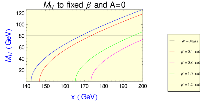
Figure 12: The masses of $H^{\pm}$ to several values of the $x$ to some fixed $\beta$ parameter here we used $A_{\lambda}=0$, the black line means the experimental values of $M_{W}$.

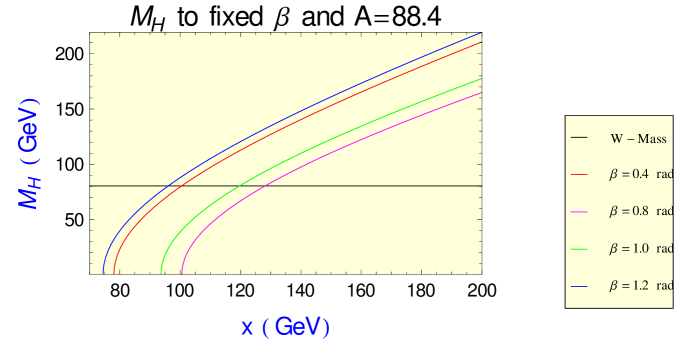
Figure 13: The masses of $H^{\pm}$ to several values of the $\beta$ to some fixed $x$ parameter here we used $A_{\lambda}=0$, the black line means the experimental values of $M_{W}$.

Figure 14: The masses of $H^{\pm}$ to several values of the $x$ to some fixed $\beta$ parameter here we used $A_{\lambda}=88.4$.

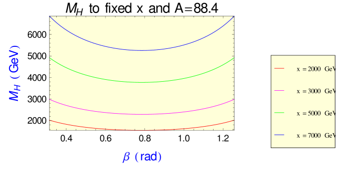
Figure 15: The masses of $H^{\pm}$ to several values of the $\beta$ to some fixed $x$ parameter here we used $A_{\lambda}=88.4$.

We notice that, when $\lambda=0$ then $\left(M^{NMSSM}_{H^{\pm}}\right)^{2}=M^{2}_{W}$. Remember that in DHM and in the MSSM the charged Higgses is always havier the $W^{\pm}$ gauge boson, see Eq.(86) and this result is agreement as presented at [65].

10.3 Pseudoscalar

We can get the mass matrix at the basis

$$\left(\begin{array}[]{ccc}\varphi_{1}&\varphi_{2}&\xi\end{array}\right)^{T}$$ (227)

and we get the matrix ${\cal M}^{2}_{CP-odd}$ and we will not write their elements here. Our first analytical result is

$$\det[{\cal M}^{NMSSM}_{CP-odd}]=0,$$ (228)

and therefore we have Goldstone boson in this sector and this result is agreement as presented at [65].

As we want to compare our result to the mass values presented at [65] we need to do the following rotation

$$\left(\begin{array}[]{c}G^{0}\\ P_{1}\\ P_{2}\end{array}\right)=\left(\begin{array}[]{ccc}\cos\beta&-\sin\beta&0\\ \cos\gamma\sin\beta&\cos\gamma\cos\beta&\sin\gamma\\ -\sin\gamma\sin\beta&-\sin\gamma\sin\beta&\cos\gamma\end{array}\right)\left(\begin{array}[]{c}\varphi_{1}\\ \varphi_{2}\\ \xi\end{array}\right),$$ (229)

where the $\tan\beta$ is defined at Eq.(74) and the new mixing angle is found to be

$$\sin\left(2\gamma\right) = -\frac{2S}{\sqrt{(T-R)^{2}+4S^{2}}},$$ (230)

$$\cos\left(2\gamma\right) = \frac{(T-R)}{\sqrt{(T-R)^{2}+4S^{2}}}.$$ (231)

We have defined

$$R = \lambda A_{\Sigma}\frac{xv^{2}}{v_{1}v_{2}},$$ (232)

$$S = \lambda v\left(A_{\Sigma}-3\kappa x\right),$$ (233)

$$T = \lambda A_{\Sigma}\frac{v_{1}v_{2}}{x}+3\kappa A_{\kappa}x+3\lambda\kappa v_{1}v_{2},$$ (234)

where we have defined

$$A_{\Sigma} = A_{\lambda}+\kappa x,$$

$$v = \sqrt{v^{2}_{1}+v^{2}_{2}}.$$ (235)

The angle $\gamma$ may be chosen as $0<\gamma<\pi$ according to [65]

$$\gamma\in\left\{\begin{array}[]{c}\left[0,\frac{\pi}{4}\right]\,\ S<0,\,\ T>R,\\ \left[\frac{\pi}{4},\frac{\pi}{2}\right]\,\ S<0,\,\ T<R,\\ \left[\frac{\pi}{2},\frac{3\pi}{4}\right]\,\ S>0,\,\ T<R,\\ \left[\frac{3\pi}{4},\pi\right]\,\ S>0,\,\ T>R.\end{array}\right.$$ (236)

The eigenvalues of ${\cal M}^{2}_{CP-odd}$ are given by:

$$M^{2}_{P_{1},P_{2}}=\frac{1}{2}\left[\left(T+R\right)\mp\sqrt{(T-R)^{2}+4S^{2}}\right],$$ (237)

where we choose $M^{2}_{P_{1}}<M^{2}_{P_{2}}$ and the eigenvectors are defined at Eq.(229) and $G^{0}$ is Goldstone boson. We show at Figs.(16,17) we can get very light pseudoscalars as required by cosmological analyses presented at [10].

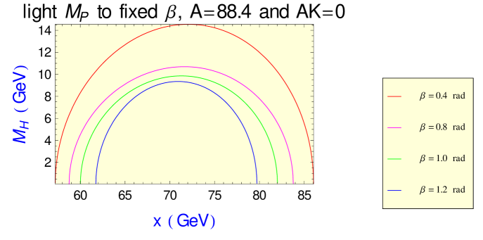
Figure 16: The masses of $P_{1}$ to several values of the $x$ to some fixed $\beta$ parameter here we used $A_{\kappa}=0$ and $A_{\lambda}=0$.

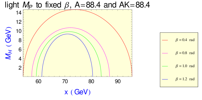
Figure 17: The masses of $P_{1}$ to several values of the $x$ to some fixed $\beta$ parameter here we used $A_{\kappa}=0$ and $A_{\lambda}=88.4$.

We can also showed, thet $P_{2}$ are heavier states than $P_{1}$, as we shown at Figs.(18,19,21).

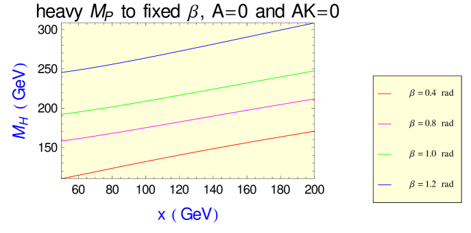
Figure 18: The masses of $P_{2}$ to several values of the $x$ to some fixed $\beta$ parameter here we used $A_{\kappa}=0$ and $A_{\lambda}=0$.

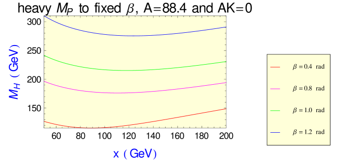
Figure 19: The masses of $P_{2}$ to several values of the $x$ to some fixed $\beta$ parameter here we used $A_{\kappa}=0$ and $A_{\lambda}=88.4$.

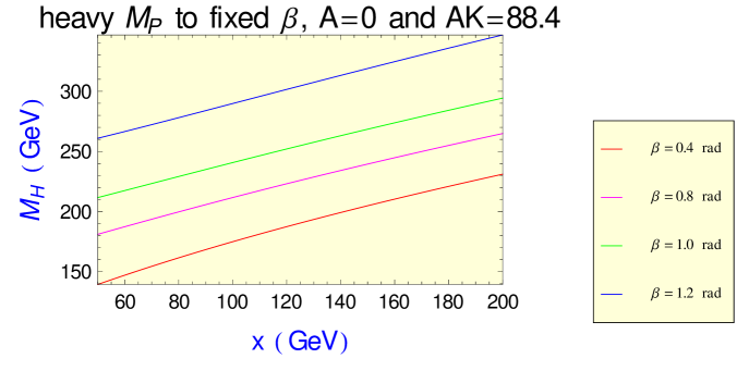
Figure 20: The masses of $P_{2}$ to several values of the $x$ to some fixed $\beta$ parameter here we used $A_{\kappa}=88.4$ and $A_{\lambda}=0$.

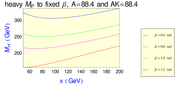
Figure 21: The masses of $P_{2}$ to several values of the $x$ to some fixed $\beta$ parameter here we used $A_{\kappa}=0$ and $A_{\lambda}=88.4$.

10.4 The Neutral Scalars

The squared mass matrix for the “scalar” neutral in the basis

$$\left(\begin{array}[]{ccc}\phi_{1}&\phi_{2}&\sigma\end{array}\right)^{T},$$ (238)

takes the form [65]

$$\lambda\left(\begin{array}[]{ccc}\frac{\bar{g}^{2}v^{2}_{1}}{\lambda}+\frac{A_{\Sigma}xv_{2}}{v_{1}}&-A_{\Sigma}x+\frac{v_{1}v_{2}}{x}(2\lambda^{2}-\bar{g}^{2})&v_{2}\left[\frac{2\lambda xv_{1}}{v_{2}}-\kappa x-A_{\Sigma}\right]\\ -A_{\Sigma}x+\frac{v_{1}v_{2}}{x}(2\lambda^{2}-\bar{g}^{2})&\frac{\bar{g}^{2}v^{2}_{2}}{\lambda}+\frac{A_{\Sigma}xv_{1}}{v_{2}}&v_{1}\left[\frac{2\lambda xv_{2}}{v_{1}}-\kappa x-A_{\Sigma}\right]\\ v_{2}\left[\frac{2\lambda xv_{1}}{v_{2}}-\kappa x-A_{\Sigma}\right]&v_{1}\left[\frac{2\lambda xv_{2}}{v_{1}}-\kappa x-A_{\Sigma}\right]&\frac{4\kappa^{2}x^{2}-\kappa A_{\kappa}x}{\lambda}+\frac{A_{\Sigma}v_{1}v_{2}}{x}\end{array}\right)$$ (239)

where we have defined

$$r \equiv \frac{x}{v},$$

$$\bar{g} \equiv \frac{1}{\sqrt{2}}\sqrt{g^{2}+g^{\prime 2}},$$ (240)

and $v$ and some others parameters of this Equation as defined at Eq.(235). It is not useful to present analytic results for the diagonalization of this matrix.

11 Neutralinos at NMSSM

The diagonal contribution to neutralinos came from the gaugino mass term given by ${\cal L}^{MSSM}_{GMT}$, while Higgsinos mass term came from the superpotential throught

$${\cal L}^{NMSSM}_{HMT} = -\lambda\left[\left(\tilde{H}_{1}\tilde{H}_{2}\right)S+\left(\tilde{H}_{1}H_{2}+H_{1}\tilde{H}_{2}\right)\tilde{S}\right]+\kappa\tilde{S}\tilde{S}S$$ (241)

$$= -\left[\lambda x\tilde{H}^{0}_{1}\tilde{H}^{0}_{2}+\lambda v_{1}\tilde{H}^{0}_{2}\tilde{S}+\lambda v_{2}\tilde{H}^{0}_{1}\tilde{S}+\kappa x\tilde{S}\tilde{S}\right]+\ldots.$$ (242)

where $\ldots$ means the terms to charged higgsinos. Using the expression to $M_{W}$ in the MSSM, we can get

$${\cal L}^{NMSSM}_{HMT} = -\left[\lambda x\tilde{H}^{0}_{1}\tilde{H}^{0}_{2}+\frac{\sqrt{2}M_{W}}{g}\lambda\left(\cos\beta\tilde{H}^{0}_{2}+\sin\beta\tilde{H}^{0}_{1}\right)\tilde{S}+\kappa x\tilde{S}\tilde{S}\right]+\ldots.$$ (243)

The mixing between higgsinos and gauginos came from Eq.(201), as the singlinos are singlet under $SU(2)_{L}\otimes U(1)_{Y}$ they can not mix with the gauginos. However the mixing between the gauginos and higgsinos, as in the MSSM, came from

$${\cal L}^{mixing}_{\tilde{H}\tilde{V}} = \sqrt{2}\imath\;\bar{H}_{1}\left(gT^{i}\lambda^{i}-\frac{g^{\prime}}{2}\lambda^{\prime}\right)\tilde{H}_{1}-\sqrt{2}\imath\;\bar{\tilde{H}}_{1}\left(gT^{i}\bar{\lambda}^{i}-\frac{g^{\prime}}{2}\overline{\lambda^{\prime}}\right)H_{1}$$ (244)

$$+ \sqrt{2}i\;\bar{H}_{2}\left(gT^{i}\lambda^{i}+\frac{g^{\prime}}{2}\lambda^{\prime}\right)\tilde{H}_{2}-\sqrt{2}i\;\bar{\tilde{H}}_{2}\left(gT^{i}\bar{\lambda}^{i}+\frac{g^{\prime}}{2}\overline{\lambda^{\prime}}\right)H_{2},$$

$$= \frac{\imath g}{\sqrt{2}}\left(v_{1}\tilde{H}^{0}_{1}\lambda^{3}+v_{2}\tilde{H}^{0}_{2}\lambda^{3}+h.c.\right)+\frac{\imath g^{\prime}}{\sqrt{2}}\left(v_{1}\tilde{H}^{0}_{1}\lambda^{\prime}+v_{2}\tilde{H}^{0}_{2}\lambda^{\prime}+h.c.\right).$$ (245)

From the MSSM is so simply to show the Eq.(225) and in similar way we can write the following expression

$$\frac{g^{\prime}v_{1}}{\sqrt{2}} = \tan\theta_{W}\frac{gv_{1}}{\sqrt{2}}=\tan\theta_{W}M_{W}\cos\beta=\tan\theta_{W}M_{Z}\cos\theta_{W}\cos\beta=M_{Z}\sin\theta_{W}\cos\beta,$$

$$\frac{g^{\prime}v_{2}}{\sqrt{2}} = \tan\theta_{W}\frac{gv_{2}}{\sqrt{2}}=\tan\theta_{W}M_{W}\sin\beta=\tan\theta_{W}M_{Z}\cos\theta_{W}\sin\beta=M_{Z}\sin\theta_{W}\sin\beta.$$ (246)

then we get

$${\cal L}^{\mbox{mixing}}_{\tilde{H}\tilde{V}} = \imath M_{Z}\left[\left(\cos\theta_{W}\cos\beta\tilde{H}^{0}_{1}+\cos\theta_{W}\sin\beta\tilde{H}^{0}_{2}\right)\lambda^{3}+\left(\sin\theta_{W}\cos\beta\tilde{H}^{0}_{1}+\sin\theta_{W}\sin\beta\tilde{H}^{0}_{2}\right)\lambda^{\prime}+h.c.\right].$$ (247)

It generate a symmetric $5\times 5$ mass matrix ${\cal M}_{0}$. In the basis

$$\psi^{0}=\left(\begin{array}[]{ccccc}-\imath\lambda^{3}&-\imath\lambda^{\prime}&\tilde{H}^{0}_{1}&\tilde{H}^{0}_{2}&\tilde{S}\end{array}\right)^{T},$$ (248)

the resulting mass terms in the Lagrangian read

$${\cal L}=-\frac{1}{2}(\psi^{0})^{T}{\cal M}_{0}(\psi^{0})+h.c.$$ (249)

where

$${\cal M}_{0}=\left(\begin{array}[]{ccccc}M_{1}&0&M_{Z}\sin\beta\cos\theta_{W}&-M_{Z}\cos\beta\cos\theta_{W}&0\\ 0&M_{2}&M_{Z}\sin\beta\cos\theta_{W}&-M_{Z}\cos\beta\cos\theta_{W}&0\\ M_{Z}\sin\beta\cos\theta_{W}&M_{Z}\sin\beta\cos\theta_{W}&0&-\frac{\lambda x}{\sqrt{2}}&-\frac{\lambda v_{2}}{\sqrt{2}}\\ -M_{Z}\cos\beta\cos\theta_{W}&-M_{Z}\cos\beta\cos\theta_{W}&-\frac{\lambda x}{\sqrt{2}}&0&-\frac{\lambda v_{1}}{\sqrt{2}}\\ 0&0&-\frac{\lambda v_{2}}{\sqrt{2}}&-\frac{\lambda v_{1}}{\sqrt{2}}&\sqrt{2}\kappa x\end{array}\right).$$ (250)

using Eq.(225) we can rewrite the elements $\left({\cal M}_{0}\right)_{3,5}$ and $\left({\cal M}_{0}\right)_{4,5}$ in the following way

$$\left({\cal M}_{0}\right)_{3,5} = \frac{\lambda v_{2}}{\sqrt{2}}=\frac{\lambda M_{Z}\cos\theta_{W}\sin\beta}{g},$$

$$\left({\cal M}_{0}\right)_{4,5} = \frac{\lambda v_{1}}{\sqrt{2}}=\frac{\lambda M_{Z}\cos\theta_{W}\cos\beta}{g},$$ (251)

using the expressions above we can write

$${\cal M}_{0}=\left(\begin{array}[]{ccccc}M_{1}&0&M_{Z}\sin\beta\cos\theta_{W}&-M_{Z}\cos\beta\cos\theta_{W}&0\\ 0&M_{2}&M_{Z}\sin\beta\cos\theta_{W}&-M_{Z}\cos\beta\cos\theta_{W}&0\\ M_{Z}\sin\beta\cos\theta_{W}&M_{Z}\sin\beta\cos\theta_{W}&0&-\frac{\lambda x}{\sqrt{2}}&-\frac{\lambda M_{Z}\cos\theta_{W}\sin\beta}{g}\\ -M_{Z}\cos\beta\cos\theta_{W}&-M_{Z}\cos\beta\cos\theta_{W}&-\frac{\lambda x}{\sqrt{2}}&0&-\frac{\lambda M_{Z}\cos\theta_{W}\cos\beta}{g}\\ 0&0&-\frac{\lambda M_{Z}\cos\theta_{W}\sin\beta}{g}&-\frac{\lambda M_{Z}\cos\theta_{W}\cos\beta}{g}&\sqrt{2}\kappa x\end{array}\right).$$ (252)

We want to stress the following [34]

• The singlino, $\tilde{S}$, does not mix directly with the gauginos, see $\left({\cal M}_{0}\right)_{1,5}$ and $\left({\cal M}_{0}\right)_{2,5}$;

• The singlino, $\tilde{S}$, mix directly with the higgsinos $\tilde{H}^{0}_{1}$ and $\tilde{H}^{0}_{2}$see $\left({\cal M}_{0}\right)_{3,5}$ and $\left({\cal M}_{0}\right)_{4,5}$;

• If $|x|\gg v_{1,2}$ the singlino decouples from the other four neutralinos, wchich will be MSSM-like;

• If $|\kappa|$ is very small this singlinolike state will become the LSP [120].

The five-by-five matrix $N$ diagonalizes, in the following way, as in the MSSM

$${\cal M}_{0}=N^{*}\,Y\,N^{-1},$$ (253)

the symmetric mass matrix ${\cal M}_{0}$ of the neutral Weyl spinors, see Eq.(253), where the eigenvalues are arranged such that $|m_{\chi^{0}_{1}}|<|m_{\chi^{0}_{2}}|<|m_{\chi^{0}_{3}}|<|m_{\chi^{0}_{4}}|<|m_{\chi^{0}_{5}}|$. The parameter $\eta_{i}$ is introduced in order to change the phase of the particle whose eigenvalue becomes negative, it means it is defined as follow

$$\eta_{i}=\left\{\begin{array}[]{c}1,m_{\chi^{0}_{i}}>0,\\ \imath,m_{\chi^{0}_{i}}<0,\end{array}\right.,\,\ i=1,\ldots 5,$$ (254)

and

$$m_{\chi^{0}_{i}}=\eta^{2}_{i}m_{\chi^{0}_{i}}.$$ (255)

The four–component notation to the neutralinos is given as

$$\tilde{\chi}^{0}_{i}=\left(\begin{array}[]{c}\chi^{0}_{i}\\ \overline{\chi^{0}_{i}}\end{array}\right),\hskip 17.07164pti=1\ldots 5.$$ (256)

We take $\lambda=0.87$, $\kappa=0.63$ as used at [65] and $x=500$ GeV and used $M=1000$ Gev and $M^{\prime}=2000$ Gev, under these parameters we get the masses of LSP is of order of $270$ GeV as shown at Fig.(22). This results is in agreement with we need to get some nice resuts in cosmological analyses as presented at [10].

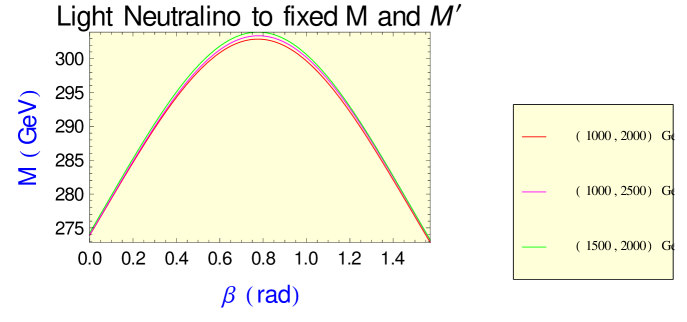
Figure 22: The masses of $\tilde{\chi}^{0}_{1}$ to several values of the $x$ to $M=1000$ Gev and $M^{\prime}=2000$ Gev as function of $\beta$ parameter.

12 Motivation to study some minimal modification

The existence of a “light” chiral gauge singlet superfield in the observable sector can cause other difficulties [34]

• The stability of gauge hierarchy;

• The superpotential of NMSSM, defined at Eq.(202), possesses a discrete ${\cal Z}_{3}$ symmetry;

however within the framework of gravity mediated SUSY breaking terms, the required amount of violation of the ${\cal Z}_{3}$ symmetry can be introduced through nonrenormalizable operators. In this context we can defined the General Singlet Extensions of the MSSM (GSEMSSM).

The most general superpotential to Singlet extension of MSSM, it can be get from super-GUT models or from super-string $E(6)$ models, is given by [64]

$$W_{GSEMSSM} = \mu\;\left(\hat{H}_{1}\hat{H}_{2}\right)+\lambda\left(\hat{H}_{1}\hat{H}_{2}\right)\hat{S}+\left(\xi_{F}M_{n}^{2}\right)\hat{S}+\frac{\mu_{2}}{2}\left(\hat{S}\right)^{2}+\frac{\kappa}{3}\left(\hat{S}\right)^{3}$$ (257)

$$+ \sum_{i,j=1}^{3}\left[\,f^{l}_{ab}\left(\hat{H}_{1}\hat{L}_{a}\right)\hat{l}^{c}_{b}+f^{d}_{ij}\left(\hat{H}_{1}\hat{Q}_{i}\right)\hat{d}^{c}_{j}+f^{u}_{ij}\left(\hat{H}_{2}\hat{Q}_{i}\right)\hat{u}^{c}_{j}\,\right].$$

The parameters $\lambda,\kappa$ and $\xi_{F}$ are dimensionless coefficients while the parameters $\mu_{2}$ and $M_{n}$ have mass dimension. Before we continue, is useful stress the following, a term of the form $M\hat{S}$ can be absorved by a shift in $\hat{S}$ [64].

We can get, from Eq.(257), the the Next-to-the-Minimal Supersymmetric Standard-Model (NMSSM) [20, 60, 61, 62, 63, 64, 66, 67], we need by setting

$$\mu=\xi_{F}=\mu_{2}=0,$$ (258)

we get the following superpotential

$$W_{NMSSM} = \lambda\left(\hat{H}_{1}\hat{H}_{2}\right)\hat{S}+\frac{\kappa}{3}\left(\hat{S}\right)^{3}+\sum_{i,j=1}^{3}\left[\,f^{l}_{ab}\left(\hat{H}_{1}\hat{L}_{a}\right)\hat{l}^{c}_{b}+f^{d}_{ij}\left(\hat{H}_{1}\hat{Q}_{i}\right)\hat{d}^{c}_{j}+f^{u}_{ij}\left(\hat{H}_{2}\hat{Q}_{i}\right)\hat{u}^{c}_{j}\,\right],$$

and the nearly Minimal Supersymmetric Model (nMSM) [121, 122], by setting

$$\mu=\mu_{2}=\kappa=0,$$ (260)

$$W_{nMSM} = \lambda\left(\hat{H}_{1}\hat{H}_{2}\right)\hat{S}+\left(\xi_{F}M_{n}^{2}\right)\hat{S}+\sum_{i,j=1}^{3}\left[\,f^{l}_{ab}\left(\hat{H}_{1}\hat{L}_{a}\right)\hat{l}^{c}_{b}+f^{d}_{ij}\left(\hat{H}_{1}\hat{Q}_{i}\right)\hat{d}^{c}_{j}+f^{u}_{ij}\left(\hat{H}_{2}\hat{Q}_{i}\right)\hat{u}^{c}_{j}\,\right].$$

Note that the nMSM differs from the NMSSM in the last term with the trilinear singlet term $\kappa$ of the NMSSM replaced by the tadpole term $\xi_{F}$ and both models have nice cosmological consequences, see for example [119, 10, 11].

12.1 Scalar Potential

The scalar potential is defined as [64]

$$V^{Dress} = M_{H_{1}}^{2}|H_{1}|^{2}+M_{H_{2}}^{2}|H_{2}|^{2}+M_{S}^{2}|S|^{2}+\left[\left(B\mu\right)\left(H_{1}H_{2}\right)+\lambda A_{\lambda}\left(H_{1}H_{2}\right)S\right.$$ (262)

$$+ \left.\frac{\left(B_{s}\mu_{2}\right)}{2}\left(S\right)^{2}+\frac{\left(\kappa A_{\kappa}\right)}{3}\left(S\right)^{3}+h.c.\right]$$

$$+ \left(|H_{1}|^{2}+|H_{2}|^{2}\right)\left|\mu+\lambda S\right|^{2}+\left|\lambda\left(H_{1}H_{2}\right)+\mu_{2}S+\kappa S^{2}\right|^{2}$$

$$+ \frac{g^{2}}{8}\left(\bar{H}_{1}\sigma^{i}H_{1}+\bar{H}_{2}\sigma^{i}H_{2}\right)^{2}+\frac{g^{\prime 2}}{8}\left(\bar{H}_{1}H_{1}-\bar{H}_{2}H_{2}\right)^{2}.$$

In this general case the mass of all scalars is given by [64]

$$M^{2}_{H^{\pm}} = M^{2}_{W}\left(1-\frac{2\lambda^{2}}{g^{2}}\right)-\frac{2C_{1}}{\sin\left(2\beta\right)},$$

compare this equation with Eq.(221). We see that both the results at NMSSM and at GSEMSSM are similar. In the case of pseudoscalar we get

$$M^{2}_{H^{PS}_{1,2}} = \frac{1}{2}\left[-\frac{2C_{1}}{\sin\left(2\beta\right)}+C_{2}\pm\sqrt{\left(\frac{2C_{1}}{\sin\left(2\beta\right)}+C_{2}\right)^{2}+\frac{16M^{2}_{W}}{g^{2}}C^{2}_{3}}\,\ \right],$$

the pseudoscalar at NMSSM is given at Eq.(237).

In Eqs.(LABEL:chargedscalaratgsemssm,LABEL:masspseudoHiggsgsemssm), we have defined the following coefficients

$$C_{1} = \lambda x\left(A_{\lambda}+\mu_{2}\right)+B\mu+\frac{\lambda\kappa}{2}x^{2},$$

$$C_{2} = -\frac{\lambda M^{2}_{W}}{g^{2}x}\left[\sin\left(2\beta\right)\left(A_{\lambda}+\mu_{2}\right)+2\mu\right]-\frac{\kappa x}{2}\left(3A_{\kappa}+\mu_{2}\right)-2B_{s}\mu_{2}-\frac{2\lambda\kappa}{g^{2}}M^{2}_{W}\sin\left(2\beta\right),$$

$$C_{3} = \lambda\left(\kappa x+\mu_{2}-A_{\lambda}\right).$$ (265)

As happen at NMSSM in this case the charged Higgs bosons can also be lighter than the $W$ boson. Note that the condition $M^{2}_{H^{PS}_{1}}\geq 0$ implies $C_{2}\geq 0$, whereas $C_{3}$ can have either sign. The interesting fact is that no absolute bound on the masses of the physical pseudoscalars can be given; in particular, $H^{PS}_{1,2}$ can both be very light. These results are in agreement with the results we presented to NMSSM, and we can in this case reproduce the masses to pseudoscalars, see Figs.(16,17) in such way that the GSEMSSM can be useful in explore cosmological analyses as presented at [10, 11].

On this case we can get an upper bound on the mass of the lighest neutral scalar $H^{0}_{1}$ and it is given by [2, 64, 34]

$$M^{2}_{H^{0}_{1}}\leq M^{2}_{Z}\left[\cos^{2}\left(2\beta\right)+\frac{2\lambda^{2}\cos^{2}\theta_{W}}{g^{2}}\sin^{2}\left(2\beta\right)\right].$$ (266)

We can show that in this model, we get the following upper bound [34]

$$M^{2}_{H^{0}_{1}}<145\,\ \mbox{GeV},$$ (267)

where $H^{0}_{1}$ is the lighest $CP$-even physical scalar and one can therefore say that supersymmetric theories always contain one neutral scalar Higgs boson with mass proportional to $M_{Z}$ [64]. To our knowledge, $200$ GeV is the absolute limit to wchich the upper bound on the lightest Higgs mass can be raised in any perturbatively treatable model with weak scale supersymmetry [34].

13 Neutralino in GSEMSSM

In the base defined at Eq.(248), the mass matrix to the neutralino masses is

$${\cal M}_{0}=\left(\begin{array}[]{ccccc}M_{1}&0&M_{Z}\sin\beta\cos\theta_{W}&-M_{Z}\cos\beta\cos\theta_{W}&0\\ 0&M_{2}&M_{Z}\sin\beta\cos\theta_{W}&-M_{Z}\cos\beta\cos\theta_{W}&0\\ M_{Z}\sin\beta\cos\theta_{W}&M_{Z}\sin\beta\cos\theta_{W}&0&-\left(\mu+\frac{\lambda x}{\sqrt{2}}\right)&-\frac{\lambda M_{Z}\cos\theta_{W}\sin\beta}{g}\\ -M_{Z}\cos\beta\cos\theta_{W}&-M_{Z}\cos\beta\cos\theta_{W}&-\left(\mu+\frac{\lambda x}{\sqrt{2}}\right)&0&-\frac{\lambda M_{Z}\cos\theta_{W}\cos\beta}{g}\\ 0&0&-\frac{\lambda M_{Z}\cos\theta_{W}\sin\beta}{g}&-\frac{\lambda M_{Z}\cos\theta_{W}\cos\beta}{g}&\sqrt{2}\kappa x+\mu_{2}\end{array}\right).$$ (268)

It is similar to Eq.(252), then we can reproduce the results presented at LSP, see Fig.(22).

14 Conclusions

In this article we have presented the MSSM and NMSSM lagrangian in terms of superfields. Then we presented the mass spectrum of those models. We shown that the masses of lighest chargino and neutralino have their masses of ${\cal O}(M_{Z})$, while the gluinos are the heavier ones, because its mass comes from SUSY soft breaking terms, and it mass is ${\cal O}(TeV)$.

We show that all the Higgs sector in the MSSM can be described in terms of $M_{A^{0}}$ and $\tan\beta$. We also showed how to get some Feynman Rules of this sector.

We have, also, presented the NMSSM and also the GSEMSSM models. We, also, show some choose of free parameter that can get the masses to pseudoscalars, see Figs.(16,17), and LSP, see Fig.(22), necessary to get the nice results in some cosmological analyses as presented at [10, 11].

We hope this review can be useful to all the people wants to learn about Supersymmetry.

Acknowledgments

The author would like to thanks to Instituto de Física Teórica (IFT-Unesp) for their nice hospitality during the period I developed this review about SUSY and from the nice workshop about Dark Matter.

The author would like to thanks to Instituto de Física Teórica (IFT-Unesp), Laboratoire de Physique Mathématique et Théorique at Université Montpellier II, Laboratório de Física Experimental at Centro Brasileiro de Pesquisas Físicas (LAFEX-CBPF), Instituto de Física da Universidade Federal do Rio Grande do Sul (IF-UFRGS) and Institut of Physics at Vietnam Academy of Science and Technology (IOP-VAST) for their nice hospitality during the period I developed some works on SUSY. Special thanks to Professores V. Pleitez, J. C. Montero, N. Berkovitz (to teach me superfields language), M. Capdequi-Peyranère, M. Manna, G. Moultaka, A. Djouadi, Jean-Loïc Kneur, Pierre Fayet, H. N. Long, P. V. Dong, D. T. Huong, C. M. Maekawa, C. B. Mariotto, J.A. Helayël-Neto and A. J. Accioly to several discussion about SUSY and also E. V. Gorbar, A. Belyaev (classes about COMPHEP) to give me the originals articles of SUSY in Russian. I would like to say thanks to Fundação de Amparo à Pesquisa do Estado de São Paulo (FAPESP), under contract number 96/10046-0 and 00/14221-9, Brazilian funding agency Conselho Nacional de Desenvolvimento Científico e Tecnológico (CNPq), under contract number 309564/2006-9 and Fundação de Amparo à Pesquisa do Estado do Rio Grande do Sul (FAPERGS), under contract number 02/1266-6, for financial support.

References

- [1] L. Susskind, Phys. Rev.D20, 2619, (1979).
- [2] J. F. Gunion, H. E. Haber, G. L. Kane and S. Dawson, The Higgs Hunter’s Guide, Front. Phys.80, 1, (2000).
- [3] N. G. Deshpande and E. Ma, Phys. Rev.D18, 2574, (1978).
- [4] H. Georgi, Hadronic J.1, 1227, (1978).
- [5] J. F. Donoghue and L. F. Li, Phys. Rev.D19, 945, (1979);
- [6] L. F. Abbott, P. Sikivie and M. B. Wise, Phys. Rev.D21, 1393, (1980);
- [7] B. McWilliams and L. F. Li, Nucl. Phys.B179, 62, (1981);
- [8] H. E. Haber, G. L. Kane and T. Sterling, Nucl. Phys.B161, 493, (1979).
- [9] J. F. Gunion and H. E. Haber, Nucl. Phys. B B272, 1, (1986); Erratum: [ Nucl. Phys.B402, 567, (1993)].
- [10] D. Hooper and T. M. P. Tait, Phys. Rev.D80, 055028, (2009); [arXiv:0906.0362 [hep-ph]].
- [11] W. Wang, Adv. High Energy Phys.2012, 216941, (2012); [arXiv:1205.5081 [hep-ph]].
- [12] P. Langacker et al., Nonstandard Higgs Bosons, Snowmass Summer Study 1984:771.
- [13] J. R. Ellis, Supersymmetry at the SSC, Snowmass Summer Study 1984:782.
- [14] A. Salam and J. A. Strathdee, Phys. Lett.B51, 353, (1974).
- [15] V. I. Ogievetskiǐ and L. Mezincescu, Sov. Phys. Usp18, 960, (1976).
- [16] J. Wess and J. Bagger, Supersymmetry and Supergravity, 2nd edition, Princeton University Press, Princeton NJ, (1992).
- [17] H. J. W. Müller-Kirsten and A. Wiedemann, SUPERSYMMETRY: AN INTRODUCTION WITH CONCEPTUAL AND CALCULATIONAL DETAILS, Second Edition, World Scientific Publishing Co. Pte. Ltd., Singapore, (2010).
- [18] A. M. Steane, An introduction to spinors, arXiv:1312.3824 [math-ph].
- [19] S. Willenbrock, Symmetries of the standard model, hep-ph/0410370.
- [20] P. Fayet, Nucl. Phys.B90, 104, (1975).
- [21] P. Fayet, Phys. Lett.B64, 159, (1976); B69, 489, (1977).
- [22] P. Fayet, Phys. Lett.B70, 461, (1977).
- [23] K. Inoue, A. Komatsu and S. Takeshita, Prog. Theor. Phys. 68, 927, (1982).
- [24] K. Inoue, A. Komatsu and S. Takeshita, Prog. Theor. Phys. 70, 330, (1983).
- [25] A. Salam and J. Strathdee, Nucl. Phys. B87, 85, (1975).
- [26] Yu. A. Gol’fand and E.P. Likhtman, ZhETF Pis. Red.13, 452, (1971) [JETP Lett.13, 323, (1971)].
- [27] D.V. Volkov and V.P. Akulov, JETP Lett.16, 438 (1972) [Pisma Zh. Eksp. Teor. Fiz.16, 621, (1972)]; Phys. Lett.B46, 109, (1973); Theor. Math. Phys. 18, 28 (1974) [Teor. Mat. Fiz. 18, 39 (1974)].
- [28] J. Wess and B. Zumino, Nucl. Phys.B70, 39, (1974); Phys. Lett.B49, 52, (1974); Nucl. Phys.B78, 1, (1974).
- [29] S. Ferrara, J. Wess and B. Zumino,Phys. Lett.51B, 239, (1974).
- [30] D. V. Volkov, Talk given at International Conference on the History of Original Ideas and Basic Discoveries in Particle Physics, Erice, Italy, 29 Jul - 4 Aug 1994, e-Print: hep-th/9410024.
- [31] G. Kane and M. Shifman, Supersymmetric World, The Beginning of the Theory, 1st edition, World Scientific Publishing Company, Singapore, (2000).
- [32] M. Shifman, The Many Faces of the Superworld: Yuri Golfand Memorial Volume, 1st edition, World Scientific Publishing Company, Singapore, (2000).
- [33] D. J. H. Chung, L. L. Everett, G. L. Kane, S. F. King, J. D. Lykken and L. T. Wang, Phys.Rept.407, 1, (2005).
- [34] M. Drees, R. M. Godbole and P. Royr, Theory and Phenomenology of Sparticles First Edition, World Scientific Publishing Co. Pte. Ltd., Singapore, (2004).
- [35] H. Baer and X. Tata, Weak scale supersymmetry: From superfields to scattering events First Edition, Cambridge University Press, Cambridge, UK, (2006).
- [36] I. J. R. Aitchison, Supersymmetry and the MSSM: An Elementary introduction, hep-ph/0505105.
- [37] H. E. Haber and G. L. Kane, Phys. Rep.117, 75, (1985).
- [38] I. Simonsen, hep-ph/9506369.
- [39] M. Kuroda, hep-ph/9902340.
- [40] S. Kraml, hep-ph/9903257.
- [41] P. Nath and R. Arnowitt, Phys. Lett. B56, 177, (1975); D. Z. Freedman, P. van Nieuwenhuizen and S. Ferrara, Phys. Rev. D13, 3214, (1976); S. Deser and B. Zumino, Phys. Lett. B62, 335, (1976).
- [42] U. Amaldi, W. de Boer, H. Fürstenau, Phys. Lett.B260, 447, (1991).
-
[43]
V. Barger, M. S. Berger and P. Ohmann, Phys. Rev. D47, 1093, (1993);
W. de Boer, R. Ehret and D. Kazakov, Z. Phys. C67, 647, (1995);
W. de Boer et al., Z. Phys. C71, 415, (1996). - [44] L. E. Ibañez and G. G. Ross, Phys. Lett.B131, 335, (1983).
- [45] B. Pendleton and G. G. Ross, Phys. Lett.B98, 291, (1981).
- [46] A. M. Sirunyan et al. [CMS Collaboration],arXiv:1805.01428 [hep-ex].
- [47] S. Dimopoulos, S. Raby and F. Wilczek, Phys. Rev.D24, 1681, (1981).
- [48] S. Dimopoulos and H. Georgi, Nucl. Phys.B193, 150, (1981).
- [49] L. E. Ibañez and G. G. Ross, Phys. Lett.B105, 439, (1981).
- [50] M. B. Einhorn and D. R. T. Jones,Nucl. Phys.B196, 475, (1982).
- [51] G. L. Kane, C. F. Kolda and J. D. Wells,Phys. Rev. Lett.70, 2686, (1993).
- [52] J. R. Espinosa and M. Quiros,Phys. Lett.B302, 51, (1993).
- [53] H. E. Haber, Eur. Phys. J.C15, 817, (2000).
- [54] A. Djouadi, Phys. Rept.459, 1, (2008).
- [55] J. A. Casas, J. R. Espinosa, M. Quiros and A.Riotto,Nucl. Phys.B436, 3, (1995); Erratum: [ Nucl. Phys.B439, 466, (1995)].
- [56] G. Aad et al. [ATLAS and CMS Collaborations],Phys. Rev. Lett.114, 191803, (2015).
- [57] P. Fayet, Nucl. Phys. Proc. Suppl.101, 81, (2001) (Also in *Minneapolis 2000, 30 years of supersymmetry* 81-98).
- [58] M. C. Rodriguez, Int. J. Mod. Phys.A25, 1091, (2010).
- [59] J. Ellis and K. A. Olive, In *Bertone, G. (ed.): Particle dark matter* 142-163; [arXiv:1001.3651 [astro-ph.CO]].
- [60] U. Ellwanger, M. Rausch de Traubenberg and C. A. Savoy, Phys. Lett.B315, 331, (1993), [arXiv:hep-ph/9307322].
- [61] S.M. Barr, Phys. Lett.B112, 219, (1982).
- [62] H. P. Nilles, M. Srednicki and D. Wyler, Phys. Lett.B120, 346, (1983).
- [63] J.-P. Derendinger and C. A. Savoy, Nucl. Phys.B 237, 307, (1984).
- [64] M. Drees, Int. J. Mod. Phys.A4, 3635, (1989). doi:10.1142/S0217751X89001448
- [65] J. R. Ellis, J. F. Gunion, H. E. Haber, L. Roszkowski and F. Zwirner, Phys. Rev.D39, 844, (1989).
- [66] B. Ananthanarayan and P. N. Pandita, Int. J. Mod. Phys.A12, 2321, (1997); [hep-ph/9601372].
- [67] U. Ellwanger and C. Hugonie, hep-ph/9901309.
- [68] M. Maniatis, Int. J. Mod. Phys.A25, 3505, (2010); [arXiv:0906.0777 [hep-ph]].
- [69] U. Ellwanger, C. Hugonie and A. M. Teixeira, Phys. Rept.496, 1, (2010); [arXiv:0910.1785 [hep-ph]].
- [70] A. Salam e J. Strathdee, Supergauge Transformations em Nucl. Phys.B76, 477, (1974).
- [71] S. Ferrara, J. Wess e B. Zumino, Supergauge Multiplets and Superfields em Phys. Lett.51B, 239, (1974).
- [72] G. Kane, Supersymmetry Squarks, Photinos, and the Unveiling of the Ultimate Laws of Nature, Primeira Edição, Helix Books, Cambridge, Massachusetts, (2000).
- [73] B.L. van der Waerden, Nachrichten Akad. Wiss. Göttingen, Math.-Physik. Kl., 100, (1929).
- [74] H.E.Haber, arXiv:hep-ph/9405376.
- [75] S. P. Martin, arXiv:1205.4076.
- [76] H. K. Dreiner, H. E. Haber, S. P. Martin,Phys. Rept.494, 1, (2010).
- [77] J. D. Lykken, hep-th/9612114.
- [78] E. Majorana, Nuovo Cim.14, 171, (1937).
- [79] P.A.M. Dirac, Proc. Royal Soc. A117, 610, (1928); 118, 351, (1928).
- [80] P. V. Dong, D. T. Huong, M. C. Rodriguez and H. N. Long,Eur. Phys. J.C48, 229, (2006).
- [81] R. Barbier et al.,Phys. Rept.420, 1, (2005).
- [82] C.M. Maekawa and M. C. Rodriguez, JHEP04, 031, (2006).
- [83] C.M.Maekawa and M.C.Rodriguez, JHEP0801, 072, (2008).
- [84] J. Ellis, J. S. Hagelin, D. V. Nanopoulos, K. Olive and M. Srednicki, Nucl. Phys.B238, 453, (1984).
- [85] J. Ellis, hep-ph/9812235.
- [86] T. Banks, Nucl. Phys.B303, 172, (1988).
- [87] L. J. Hall and M. Suzuki, Nucl. Phys.B231, 419, (1984).
- [88] M. A. Diaz, J. C. Romão and J. W. F. Valle, Nucl. Phys.B524, 23, (1998).
- [89] F. Borzumati and Y. Nomura, Phys. Rev.D64, 053005, (2001); F. Borzumati, K. Hamaguchi and T. Yanagida, Phys. Lett.B497, 259, (2001); F. Borzumati, K. Hamaguchi, Y. Nomura and T. Yanagida, hep-ph/0012118.
- [90] R. N. Mohapatra, Phys. Rev.D34, 3457, (1986).
- [91] J. C. Romão and J. W. F. Valle, Nucl. Phys.B381, 87, (1992).
- [92] S. Davison and M. Losada, hep-ph/0010325.
- [93] J. C. Montero, V. Pleitez and M. C. Rodriguez, Phys. Rev.D65, 095008, (2002).
- [94] L. Girardello and M. T. Grisaru, Nucl. Phys. B194, 65, (1982).
- [95] M. Srednicki, Quantum field theory, Fourth Edition, Cambridge University Press, United Kindom, (2010); and also avaliable at arXiv:hep-th/0409035 and arXiv:hep-th/0409036.
- [96] J. L. Kneur and G. Moultaka, Phys. Rev.D59, 015005, 1999.
- [97] C. B. Mariotto and M. C. Rodriguez,arXiv:0805.2094 [hep-ph].
- [98] S. Dawson, E. Eichten and C. Quigg, Phys. Rev.D31, 1581, (1985).
- [99] D. B. Espindola, M. C. Rodriguez and C. B. Mariotto,Braz. J. Phys.43, 105, (2013).
- [100] C. Brenner Mariotto, D. B. Espindola and M. C. Rodriguez,Phys. Rev.C83, 064902, (2011).
- [101] D. B. Espindola, C. Brenner Mariotto and M. C. Rodriguez,AIP Conf. Proc.1296, 262, (2010).
- [102] S. Heinemeyer and C. Schappacher,Eur. Phys. J.C72, 1905, (2012).
- [103] E. Ma, Phys. Rev.D39, 1922, (1989).
- [104] A. Bartl, H. Fraas, W. Majerotto and B. Mößlacher, Z. Phys.C55, 257, (1992).
- [105] A. Bartl, H. Fraas and W. Majerotto, Nucl. Phys.B278, 1, (1986).
- [106] M. Guchait, Z. Phys.C57, 157, (1993); Erratum C67, 178, (1994).
- [107] H. E. Haber and R. Hempfling, Phys. Rev. Lett.66,1815, (1991).
- [108] M. Carena, J. Ellis, J. S. Lee, A. Pilaftsis and C. E. M. Wagner, arXiv:1512.00437.
- [109] M. Glück and E. Reya, Phys. Rev.D31, 620, (1985).
- [110] H. Baer, C. h. Chen, F. Paige and X. Tata, Phys. Rev.D49, 3283, (1994).
- [111] A. Bartl, H. Fraas and W. Majerotto, Z. Phys.C34, 411, (1987).
- [112] A. Bartl, H. Fraas and W. Majerotto, Nucl. Phys.B297, 479, (1988).
- [113] D. B. Espindola, C. B. Mariotto and M. C. Rodriguez,AIP Conf. Proc.1520, 273, (2013).
- [114] B.C. Allanach et al, Eur.Phys.J.C25, 113, (2002).
- [115] Nabil Ghodbane and Hans-Ulrich Martyn, hep-ph/0201233.
- [116] S. Y. Choi, Y. S. Shim, H. S. Song and W. Y. Song, hep-ph/9808227.
- [117] T. Takagi, Japan J. Math1, 83, (1925).
- [118] R. A. Horn and C. R. Johnson, Matrix Analysis, first edition, Cambridge University Press, Cambridge, UK, (1990).
- [119] M. C. Rodriguez and I. V. Vancea, arXiv:1603.07979 [hep-ph].
- [120] U. Ellwanger, M. Rausch de Traubenberg and C. A. Savoy, Nucl. Phys.B492, 21, (1997).
- [121] C. Panagiotakopoulos, K. Tamvakis, Phys. Lett.B446, 224, (1999); Phys. Lett.B469, 145, (1999); C. Panagiotakopoulos, A. Pilaftsis, Phys. Rev.D63, 055003, (2001); A. Dedes, C. Hugonie, S. Moretti and K. Tamvakis, Phys. Rev.D63, 055009, (2001); A. Menon, D.E. Morrissey, C.E.M. Wagner, Phys. Rev.D70, 035005, (2004); V. Barger, P. Langacker and H. S. Lee, Phys. Lett.B630, 85, (2005); C. Balazs, M. Carena, A. Freitas and C. E. M. Wagner, JHEP0706, 066, (2007); J. Cao, Z. Heng and J. M. Yang, JHEP1011, 110, (2010).
- [122] J. Cao, H. E. Logan, J. M. Yang, Phys. Rev.D79, 091701, (2009).