Time in quantum mechanics:
A fresh look on quantum hydrodynamics and quantum trajectories

Abstract

Quantum hydrodynamics is a formulation of quantum mechanics based on the probability density and flux (current) density of a quantum system. It can be used to define trajectories which allow for a particle-based interpretation of quantum mechanics, commonly known as Bohmian mechanics. However, quantum hydrodynamics rests on the usual time-dependent formulation of quantum mechanics where time appears as a parameter. This parameter describes the correlation of the state of the quantum system with an external system – a clock – which behaves according to classical mechanics. With the Exact Factorization of a quantum system into a marginal and a conditional system, quantum mechanics and hence quantum hydrodynamics can be generalized for quantum clocks. In this article, the theory is developed and it is shown that trajectories for the quantum system can still be defined, and that these trajectories depend conditionally on the trajectory of the clock. Such trajectories are not only interesting from a fundamental point of view, but they can also find practical applications whenever a dynamics relative to an external time parameter is composed of “fast” and “slow” degrees of freedom and the interest is in the fast ones, while quantum effects of the slow ones (like a branching of the wavepacket) cannot be neglected. As an illustration, time- and clock-dependent trajectories are calculated for a model system of a non-adiabatic dynamics, where an electron is the quantum system, a nucleus is the quantum clock, and an external time parameter is provided, e.g. via an interaction with a laser field that is not treated explicitly.

Although being developed for ca. 100 years, the meaning of quantum mechanics is still a topic of active discussion. Next to the open question of merging quantum mechanics with general relativity,isham1993 ; anderson2017 ; bose2017 ; carney2019 the development of first usable quantum computers preskill2018 has recently sparked interest in the fundamentals of the theory and questions like its consistent use attracted some attention.frauchiger2018 ; lazarovici2019 During the years, several formulations and interpretations of quantum mechanics have been proposed.styer2002 While they all may reproduce the known experimental results, some of them are useful beyond philosophical questions while others have so far been of little use other than for entertaining debates. Two closely related formulations of the former type are quantum hydrodynamics and Bohmian mechanics,madelung1926 ; madelung1927 ; broglie1927 ; bohm1952 ; bohm1952_2 which both suggest strategies for calculating properties of larger quantum systems. Here, these two formulations are re-considered in the light of the emergence of the concept of time in quantum mechanics.

The standard approach to non-relativistic quantum mechanics is based on the time-dependent Schrödinger equation (TDSE) that describes the state of a quantum system by means of a wavefunction. It is the central quantity of the theory and contains all relevant information that is needed to compute observables of the quantum system. The wavefunction changes as time passes and, in this way, the state evolves. However, there are at least two problems with the theory of quantum mechanics: The first problem is the “measurement problem”, as the act of measuring the quantum system is usually treated as additional postulate.bell1990 ; hollowood2016 ; landsman2017 An interaction with an external system, the measurement apparatus, leads to a “collapse” of the wavefunction into the state corresponding to the measurement outcome. The second problem is the “time problem”, as time in the TDSE is not a quantum-mechanical observable but a parameter which leads to conceptual challenges like the definition of a tunneling time steinberg1995 ; landsman2015 ; zimmermann2016 ; sokolovski2018 or the unification of quantum mechanics with general relativity.isham1993 ; anderson2017 Both the measurement problem and the time problem are rooted in an inconsistent treatment of the quantum system and its (external) environment.

Two useful alternatives to a wavefunction-based picture can be obtained by writing the complex-valued wavefunction of a quantum system in its polar form. Then, equations of motion follow for a probability density and probability flux (current) density. These equations are similar in appearance to the equations of motion of fluid dynamics, hence they are known as quantum hydrodynamics madelung1926 ; madelung1927 and have found several applications, e.g. in the study of Bose-Einstein condensatestsubota2013 or in plasma physics.shukla2011 ; moldabekov2018 Recently, the extension of quantum hydrodynamics to many-particle systems has also been studied in detail.renziehausen2018

Closely related to quantum hydrodynamics is the De Broglie-Bohm interpretation of quantum mechanics, also known as Bohmian mechanics, where particles are assumed to follow trajectories with a velocity field that is determined by the wavefunction.broglie1927 ; bohm1952 ; bohm1952_2 Bohmian mechanics is conceptually attractive for several reasons, e.g. because some consider it not to have the measurement problem.durr1992 ; durr2004_2 ; norsen2016 For practical applications, Bohmian mechanics can be viewed as trajectory-based quantum hydrodynamics, and in the last years a number of studies have appeared that aim at using these quantum trajectories to develop simulation methods, in particular for molecular dynamics wyatt2001 ; lopreore2002 ; wyatt2005 ; rassolov2005 ; curchod2013 ; agostini2018 , also by extending it to complex-valued trajectories goldfarb2006 ; zamstein2012 ; zamstein2012_2 ; koch2017 or by using the “conditional wavefunction” approach oriols2007 ; benseny2014 ; albareda2014 ; albareda2016 .

Both quantum hydrodynamics and Bohmian mechanics are derived from a time-dependent description of quantum mechanics. Hence, although Bohmian mechanics might not have the measurement problem, it does have the time problem. While the time problem is often not a problem in practice, it is assumed to be major theoretical problem for the unification of quantum mechanics with the general theory of relativity.isham1993 ; anderson2017 A few solutions have been proposed, e.g. the Page-Wootters approach,page1983 ; wootters1984 which gained some interest recently,moreva2014 ; moreva2015 ; giovannetti2015 ; moreva2017 ; marletto2017 ; bryan2018 ; smith2019 or an approach based on the Born-Oppenheimer approximation, which was applied to gravity and matter banks1985 ; brout1987 ; englert1989 and which has also been considered by Briggs and Rost a few years ago.briggs2000 Additionally, time in general relativity has been reconsidered and there are promising developments like shape dynamics barbour2014a ; barbour2014b that illuminate the meaning of time as a correlation. All these show that the concept of an external time parameter needs to be replaced with the explicit consideration some part of the system as the “clock” that is used to define time.

Here, we use an extension of the developments made by Briggs and Rost briggs2000 and by Briggs and coworkers braun2004 ; briggs2014 ; briggs2015 to derive the time parameter in quantum mechanics. With the help of this approach, it can be shown that “time” appearing in the TDSE has a similar status like the measurement apparatus in standard quantum mechanics: It is not truly part of the theory. Instead, it is a Newtonian time parameter $t$ that describes the correlation of the state of the quantum system relative to an external system, the clock, which provides $t$. To be able to do that, the clock needs to behave according to classical mechanics so that e.g. its position and velocity are known and can be used to define $t$.

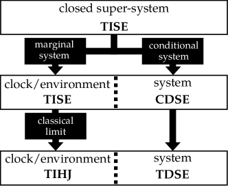
Figure 1: Schematic representation of the steps needed to derive time in quantum mechanics: By separating a closed super-system described by a time-independent Schrödinger equation (TISE) into a marginal part (clock) and a conditional part (system), it is found that the clock obeys an effective TISE and the system obeys a clock-dependent Schrödinger equation (CDSE). If a classical limit is taken for the clock, it obeys a time-independent Hamilton-Jacobi equation (TIHJ); the CDSE for the system system then becomes a time-dependent Schrödinger equation (TDSE) for a time-parameter defined via the classical clock.

Explicitly, the time-dependence of the TDSE can be derived from a time-independent description of a super-system which is being partitioned into the actual system of interest and the clock,briggs2000 ; briggs2015 ; schild2018 as indicated in Figure 1. The super-system is assumed to be closed and hence is described by a time-independent Schrödinger equation (TISE). To introduce the concept of time in this time-independent description, a part of the super-system is considered to be a marginal part, i.e., its state is being described after averaging over the rest of the super-system. This part is the clock, but it may also be viewed as an environment. The state of the rest of the super-system, which is the actual system of interest, is then conditionally depended on the state of the clock. If a classical limit for the clock is taken, its equation of motion becomes a classical time-independent Hamilton-Jacobi equation. A time parameter can then be defined along the classical trajectory of the clock, and the equation of motion for the system of interest becomes a TDSE.briggs2015 It follows that, because time in the TDSE is defined via a classical clock, the TDSE is actually a semi-classical equation. For the same reason, also quantum hydrodynamics as well as Bohmian mechanics are semi-classical theories.

The formalism for separating the quantum super-system into a marginal part and a conditional part is called the Exact Factorization,abedi2010 ; abedi2012 which can be viewed as a rigorous extension of ideas from the Born-Oppenheimer approximation.born1927 If the classical limit for the clock is not taken, a fully quantum-mechanical equation of motion for the system is obtained from the Exact Factorization. We call this equation the clock-dependent Schrödinger equation (CDSE) schild2018 because the state of the quantum system does not depend conditionally on a classical time parameter, like in the TDSE, but on the state of the quantum clock. Instead of an unobservable time parameter, only observable quantities like the configuration and momentum of the clock appear in the CDSE.

In this article, we investigate how the equations of quantum hydrodynamics change if, instead of the TDSE, the CDSE is used as starting point for its derivation. For this purpose, in section I we explain what is meant with the classical limit and in section II we provide a brief review of the basis of time-dependent quantum hydrodynamics and explain how the trajectory-based picture of Bohmian mechanics can be derived. Thereafter, in section III the CDSE is introduced which is used, in section IV, to derive clock-dependent quantum hydrodynamics and a clock-dependent trajectory picture. To illustrate these trajectories, a simple model of an electron dynamics with a quantum nucleus and an external time parameter is presented in section V. Finally, in section VI some implications and possible applications of clock-dependent quantum hydrodynamics are discussed.

The notation in the following is such that similar quantities are denoted with similar symbols. However, to avoid notational clutter the symbols may be re-defined in different parts of the text. Care is taken to define the symbols correctly, but the preceding definitions need to be considered if equations of different parts of the text are to be compared. In particular, same symbols with different dependencies may refer to different (but related) quantities.

I The classic limit

Below, in several occasions a classical limit of quantum mechanics is mentioned. In this section, it is briefly explained in which sense this classical limit is to be understood here (see e.g. klein2012 for a critical discussion). The evolution of a single-particle quantum system described by its state function $\varphi(\bm{x}|t)\in\mathbb{C}$ is given by the TDSE

$$i\hbar\partial_{t}\varphi(\bm{x}|t)=\left(\frac{\bm{\hat{p}}^{2}}{2m}+V(\bm{x},t)\right)\varphi(\bm{x}|t)$$ (1)

where $\bm{\hat{p}}=-i\hbar\nabla_{\bm{x}}$ is the momentum operator, $m$ is the mass of the particle, $t\in\mathbb{R}$ is the time parameter, $\partial_{t}$ is the derivative w.r.t. $t$, $\bm{x}\in\mathbb{R}^{3}$ is the position of the particle and $\nabla_{\bm{x}}$ is the gradient w.r.t. $\bm{x}$. For simplicity, we assume that there is only a scalar potential $V(\bm{x},t)$ that represents the interaction with the environment of the particle, and that no vector potential is present. We write

$$\varphi(\bm{x}|t)=e^{iz(\bm{x}|t)/\hbar}$$ (2)

and expand the action $z$ in powers of $\hbar$,

$$z(\bm{x}|t) =\sum_{j=0}^{\infty}\hbar^{j}z^{(j)}(\bm{x}|t).$$ (3)

In principle, for such an expansion a dimensionless parameter should be chosen instead of $\hbar$. The difference between using such a parameter and using $\hbar$ seems to be largely irrelevant in single-particle quantum mechanics but can be important for multi-particle systems where the classical limit is only made for a part of the total system. Then, a suitable parameter is needed which effectively becomes a pre-factor for those appearances of $\hbar$ that actually relate to the part for which the classical limit is made. Below, such a partial classical limit is discussed for a clock as part of a quantum super-system, but for simplicity we limit the discussion here to an expansion in terms of $\hbar$. Details about how to perform the classical limit correctly for the case discussed below can be found in eich2016 .

To lowest order in $\hbar$, we find

$$0 =\partial_{t}s+\frac{\left(\nabla_{\bm{x}}s\right)^{2}}{2m}+V$$ (4)

with $s(\bm{x}|t)\equiv z^{(0)}\in\mathbb{R}$ being real-valued. This is a classical Hamilton-Jacobi equation with classical momentum $\nabla_{\bm{x}}s$, hence it can be viewed as classical limit of the quantum problem. Interestingly, as $s$ is (chosen) real-valued, the wavefunction to lowest order in $\hbar$ corresponds to a constant probability density, $|\varphi^{(0)}(\bm{x}|t)|^{2}=|e^{is}|^{2}=1$. The quantum properties of the system arise from a confinement (due to interaction with other particles) which is represented by a variation of the density. We find the correction to first order in $\hbar$ from

$$\partial_{t}w =-\frac{\nabla_{\bm{x}}s\nabla_{\bm{x}}w}{m}-\frac{\nabla_{\bm{x}}^{2}s}{2m}$$ (5)

with $w(\bm{x}|t)=iz^{(1)}\in\mathbb{R}$. This correction provides such a variation of the density, $|\varphi^{(1)}(\bm{x}|t)|^{2}=|e^{w+is}|^{2}=e^{2w}$.

To conclude the short discussion of the classical limit, we note that if we had started from a TISE

$$E\varphi(\bm{x}|t)=\left(\frac{\bm{\hat{p}}^{2}}{2m}+V(\bm{x},t)\right)\varphi(\bm{x}|t)$$ (6)

with energy $E$, the classical limit would correspond to the time-independent Hamilton-Jacobi equation

$$E =\frac{(\nabla_{\bm{x}}s)^{2}}{2m}+V.$$ (7)

This classical limit is needed below because we discuss a closed (and hence time-independent) super-system to define time internally as correlation of a part of the super-system to another part, which serves as the clock. The trajectories of a classical clock are then given as solutions of (7).

II Time-dependent quantum hydrodynamics

The hydrodynamic formulation of quantum mechanics madelung1926 ; madelung1927 for a single-particle system is obtained from the TDSE (1) by writing the complex number $\varphi$ in its polar form,

$$\varphi(\bm{x}|t) =\sqrt{\rho(\bm{x}|t)}e^{is(\bm{x}|t)}$$ (8)

$$=e^{w(\bm{x}|t)+is(\bm{x}|t)}$$ (9)

with probability density $\rho(\bm{x}|t)=|\varphi(\bm{x}|t)|^{2}\in\mathbb{R}$ and with real-valued dimensionless action $s\in\mathbb{R}$. In (9), also a second real-valued dimensionless action $w\in\mathbb{R}$ is introduced which may be used instead of the probability density $\rho$. By inserting (8) into the TDSE (1) and by separating the result into real and imaginary parts, two equations are obtained. The first of these equations is a Hamilton-Jacobi equation,

$$0=\hbar\partial_{t}s(\bm{x}|t)+H(\bm{p},\bm{x}|t),$$ (10)

where

$$H(\bm{p},\bm{x}|t) =\frac{\bm{p}(\bm{x}|t)^{2}}{2m}+V(\bm{x}|t)+u(\bm{x}|t)$$ (11)

is a Hamiltonian function,

$$\bm{p}(\bm{x}|t)=\hbar\nabla_{\bm{x}}s(\bm{x}|t)$$ (12)

is a real-valued momentum field, and $u(\bm{x}|t)$ is the so-called quantum potential

$$u(\bm{x}|t)=-\frac{1}{2m}\left(\bm{\hat{p}}_{\rm c}\cdot\bm{\pi}(\bm{x}|t)+\bm{\pi}(\bm{x}|t)^{2}\right)$$ (13)

that vanishes if a suitable classical limit is taken for $\varphi(\bm{x}|t)$. In the expression for the quantum potential (13) we used the operator

$$\bm{\hat{p}}_{\rm c} =i\bm{\hat{p}}=\hbar\nabla_{\bm{x}}$$ (14)

and the quantity

$$\bm{\pi}(\bm{x}|t)=\frac{\hbar\nabla_{\bm{x}}\rho}{2\rho}=\hbar\nabla_{\bm{x}}w(\bm{x}|t),$$ (15)

which is another real-valued momentum field, $\bm{\pi}\in\mathbb{R}$ (also used e.g. in garashchuk2014 ; gao2017 ). It represents the relative variation $\frac{\nabla_{\bm{x}}\rho}{\rho}$ of the density with position $\bm{x}$. The second of the equations obtained from (8) and (1) is the continuity equation

$$0=\partial_{t}\rho(\bm{x}|t)+\nabla_{\bm{x}}\cdot\bm{j}(\bm{x}|t)$$ (16)

with probability flux (current) density

$$\bm{j}(\bm{x}|t)=\rho(\bm{x}|t)\frac{\bm{p}(\bm{x}|t)}{m}.$$ (17)

The continuity equation (16) represents the conservation of the probability density $\rho(\bm{x}|t)$. It essentially states that in any volume $\Omega$, the change of density $\partial_{t}\rho(\bm{x}|t)$ is given by the flow of density through the boundary of $\Omega$, and that flow is determined by the probability flux density $\bm{j}(\bm{x}|t)$.aris1989 For comparison with the development presented below, it is also useful to express (16) with the momentum field $\bm{\pi}$, i.e., the continuity equation is equivalent to

$$0 =\hbar^{2}\partial_{t}w+\frac{1}{m}\left(\bm{\pi}\cdot\bm{p}+\frac{\bm{\hat{p}}_{\rm c}\cdot\bm{p}}{2}\right)=\hbar^{2}\nabla_{\bm{r}}w+\frac{\nabla_{\bm{x}}\cdot\bm{j}}{2\rho}.$$ (18)

While version (16) of the continuity equation contains quantities that are non-zero only in regions where the particle actually can be found (in the sense of its probability distribution), version (18) relates quantities that can be sizable everywhere.

To obtain the particle-based interpretation of quantum mechanics known as Bohmian mechanics, it is necessary to solve the Hamilton-Jacobi equation (10) with the method of characteristics.agostini2018 By using this method, (10) is interpreted as differential equation for the phase $s(\bm{x}|t)$ alone, i.e., it is assumed that the quantum potential $u(\bm{x}|t)$ (or the density $\rho(\bm{x}|t)$, or $w(\bm{x}|t)$) is known. Then, (10) is solved along parametrized curves. It turns out that the parameter can be identified with $t$ and that the curves can be obtained by solving

$$\partial_{t}\bm{x}_{\rm t}(t) =\frac{\bm{p}_{\rm t}(t)}{m}$$ (19)

$$\partial_{t}\bm{p}_{\rm t}(t) =-\nabla_{\bm{x}}H(\bm{p}_{\rm t}(t),\bm{x}_{\rm t}(t)|t)$$ (20)

$$\partial_{t}S_{\rm t}(t) =\frac{\left(\bm{p}_{\rm t}(t)\right)^{2}}{m}-H(\bm{p}_{\rm t}(t),\bm{x}_{\rm t}(t)|t).$$ (21)

Here, $\bm{x}_{\rm t}$, $\bm{p}_{\rm t}$, and $S_{\rm t}$ are the values of $\bm{x}$, $\bm{p}$, and $S$ along the trajectory, respectively.

From (19) it is possible to interpret the curves $\bm{x}_{\rm t}(t)$ as trajectories of the particle which are guided by the wavefunction $\varphi(\bm{x}|t)$ via the momentum field $\bm{p}(\bm{x}|t)$ or, if the momentum field is computed from (20), via the quantum potential $u(\bm{x}|t)$ appearing in the Hamiltonian function $H$. If several trajectories are considered with their initial locations $\bm{x}_{\rm t}(t_{0})$ randomly sampled according to $\rho(\bm{x}|t_{0})$ at some time $t_{0}$, or if the trajectories are equally spaced but carry a weight according to this distribution, the continuity equation (16) ensures that the trajectories yield the distribution $\rho(\bm{x}|t)$ for any time $t$. Hence, the basic equations of quantum hydrodynamics may be interpreted as giving rise to a particle picture of quantum mechanics where the particles have a definite trajectory in space, but the trajectories are guided by the phase of the wavefunction (or the quantum potential) and distributed according to its squared magnitude.

It has to be noted that a few unusual conventions were chosen in the preceding discussion of time-dependent quantum hydrodynamics. First, it is custom to divide $w$ and $s$ by $\hbar$ in the ansatz (8), so as to give them units of action. We made this choice above when discussion the classical limit. It is convenient for single-particle quantum mechanics but less convenient for the treatment presented below where vector potentials appear, hence it is not done here.

Second, momentum fields are considered, which is typically done for the Hamilton-Jacobi equation but which is in contrast to much literature on quantum hydrodynamics and Bohmian mechanics, where a formulation of the equations in terms of velocity fields tends to be preferred. The preference might originate from the fact that the velocity field $\frac{\bm{p}(\bm{x}|t)}{m}$ occurs in the definition of the flux density $\bm{j}(\bm{x}|t)$ (17) and in the guiding equation (19) of Bohmian mechanics, and it also prevents confusion with the momentum operator $\bm{\hat{p}}$. That momentum fields are considered here is because of this authors subjective choice, but a reformulation in terms of velocity fields is straightforward.

Third, the quantum potential is usually given as

$$u(\bm{x}|t)=-\frac{\hbar^{2}}{2m}\frac{\nabla_{\bm{x}}^{2}|\varphi|}{|\varphi|}$$ (22)

and the momentum field $\bm{\pi}(\bm{x}|t)$ is not introduced. However, if time is replaced by a quantum clock, it is more convenient to work with the two momentum fields $\bm{p}$ and $\bm{\pi}$ than with other quantities like the density $\rho$ and flux density $\bm{j}$ in the sense that the equations become more transparent, even though the densities have the virtue of being of relevant magnitude only in regions where the particle can actually be found. In the classical limit corresponding to (4), the momentum field $\bm{p}$ becomes the classical momentum while the momentum field $\bm{\pi}$ (and hence the quantum potential $U$) vanish. We will thus call $\bm{p}$ the classical momentum field and $\bm{\pi}$ the quantum momentum field in the following. Also, using $\bm{\pi}(\bm{x}|t)$ makes the quantum potential look (partially) like an additional kinetic energy term. As explained in section I, the variation of the density (which is what $\bm{\pi}$ represents) is a sign of “quantum behavior” of the system, but it also reflects an effective interaction with other particles that are not treated explicitly but only implicitly via a scalar potential $V$ or a vector potential. Hence, the quantum potential may loosely be interpreted as effective reaction of the system on its confinement.

III The clock-dependent Schrödinger equation

As stated above, the TDSE is a semi-classical description of a quantum system because its time parameter originates from an implicit comparison of the state of the quantum system to the state of a classical clock. A quantum mechanical generalization of the TDSE, the CDSE, can be obtained as follows:schild2018 The state $\psi(\bm{R},\bm{r})$ of a super-system composed of two parts is determined by the TISE

$$\left(\frac{\bm{\hat{P}}^{2}}{2M}+\frac{\bm{\hat{p}}^{2}}{2m}+V(\bm{R},\bm{r})\right)\psi(\bm{R},\bm{r})=E\psi(\bm{R},\bm{r}),$$ (23)

where $\bm{\hat{P}}=-i\hbar\nabla_{\bm{R}}$ and $\bm{\hat{p}}=-i\hbar\nabla_{\bm{r}}$ are two momentum operators and $V(\bm{R},\bm{r})$ is a scalar potential. This equation is written for two particles with coordinates $\bm{R}$ and $\bm{r}$ and masses $M$ and $m$, respectively, but it can be generalized to any number of particles by replacing the two kinetic energy operators that occur in (23) with sums of such operators. Also, the momentum operators $\bm{\hat{P}}$ and $\bm{\hat{p}}$ may include vector potentials without changing the results discussed below in any relevant way. Next, the joint probability density $|\psi(\bm{R},\bm{r})|^{2}$ is written as product

$$|\psi(\bm{R},\bm{r})|^{2}=|\chi(\bm{R})|^{2}|\phi(\bm{r}|\bm{R})|^{2},$$ (24)

where

$$|\chi(\bm{R})|^{2}:=\Braket{\psi(\bm{R},\bm{r})}{\psi(\bm{R},\bm{r})}$$ (25)

is the marginal probability density of finding the particle of mass $M$ at $\bm{R}$ independent of where the particle of mass $m$ is. The symbol $\Braket{\cdot}$ indicates integration over the coordinates $\bm{r}$ and $\Braket{a}{b}=\Braket{\bar{a}b}$ is the complex-valued scalar product, where $\bar{a}$ is the complex-conjugate of $a$. The function $\chi(\bm{R})$ is called marginal amplitude or marginal wavefunction and its phase can be chosen arbitrarily (which leads to a gauge freedom in the theory, as discussed below). The probability density $|\phi(\bm{r}|\bm{R})|^{2}$ is the conditional probability density for finding the particle with mass $m$ at $\bm{r}$ given the particle with mass $M$ is at $\bm{R}$. The conditional amplitude or conditional wavefunction is defined as

$$\phi(\bm{r}|\bm{R}):=\frac{\psi(\bm{R},\bm{r})}{\chi(\bm{R})}$$ (26)

and, if $\psi(\bm{R},\bm{r})$ is normalized according to

$$\int\Braket{\psi(\bm{R},\bm{r})}{\psi(\bm{R},\bm{r})}d\bm{R}\stackrel{{\scriptstyle!}}{{=}}1,$$ (27)

it needs to obey the partial normalization condition

$$\Braket{\phi(\bm{r}}{\bm{R})}{\phi(\bm{r}|\bm{R})}\stackrel{{\scriptstyle!}}{{=}}1$$ (28)

for all $\bm{R}$, as is required for a conditional probability. Then, the marginal amplitude is normalized as

$$\int|\chi(\bm{R})|^{2}d\bm{R}=1.$$ (29)

The idea to write the wavefunction as a product of a marginal and a conditional wavefunction was brought up some time ago hunter1975 and has recently been developed further under the name Exact Factorization.abedi2010 ; abedi2012 The equations of motion for $\chi(\bm{R})$ and $\phi(\bm{r}|\bm{R})$ that follow are

$$E\chi =\left(\frac{(\bm{\hat{P}}+\bm{A}(\bm{R}))^{2}}{2M}+\epsilon(\bm{R})\right)\chi$$ (30)

$$\hat{C}\phi =\left(\frac{\bm{\hat{p}}^{2}}{2m}+V(\bm{R},\bm{r})+\hat{U}-\epsilon(\bm{R})\right)\phi$$ (31)

with scalar and vector potentials

$$\epsilon(\bm{R}) :=\Braket{\phi}{\frac{\bm{\hat{p}}^{2}}{2m}+V(\bm{R},\bm{r})+\hat{U}-\hat{C}}{\phi}$$ (32)

$$\bm{A} :=\Braket{\phi}{\bm{\hat{P}}\phi},$$ (33)

with the kinetic operator

$$\hat{U} =\frac{(\bm{\hat{P}}-\bm{A})^{2}}{2M}$$ (34)

and with the coupling operator

$$\hat{C} =-\frac{1}{M}\frac{(\bm{\hat{P}}+\bm{A})\chi(\bm{R})}{\chi(\bm{R})}\cdot\left(\bm{\hat{P}}-\bm{A}\right)$$ (35)

that depends explicitly on the wavefunction $\chi(\bm{R})$. The choice of the phase of $\chi(\bm{R})$ is a gauge freedom, i.e., the transformation

$$\chi^{\prime}(\bm{R}) =\chi(\bm{R})e^{-i\theta(\bm{R})}$$ (36)

$$\phi^{\prime}(\bm{r}|\bm{R}) =\phi(\bm{r}|\bm{R})e^{i\theta(\bm{R})}$$ (37)

$$\bm{A}^{\prime}(\bm{R}) =\bm{A}(\bm{R})+\nabla_{\bm{R}}\theta(\bm{R})$$ (38)

leaves the total wavefunction $\psi(\bm{R},\bm{r})$ as well as all equations of motion in the theory invariant.

The marginal wavefunction $\chi(\bm{R})$ is interpreted as the wavefunction of the clock or environment, whereas the conditional wavefunction $\phi(\bm{r}|\bm{R})$ is the wavefunction of the quantum system of interest. It has been shown that if the clock behaves classical, the equation of motion for $\chi(\bm{R})$ becomes the analogue of the time-independent Hamilton-Jacobi equation (7).briggs2000 ; briggs2015 ; eich2016 ; schild2018 Solving this equation for its characteristics yields classical trajectories. The corresponding classical configuration and momentum of the clock along these trajectories can be parametrized with a variable $t$ which may be interpreted as time parameter. In the equation of motion for $\phi(\bm{r}|\bm{R})$, the contribution of the operator $\hat{U}$ vanishes, the clock-dependent operator becomes

$$\hat{C}\rightarrow i\hbar\bm{V}_{\rm cl}\nabla_{\bm{R}_{\rm cl}}\rightarrow i\hbar\partial_{t}$$ (39)

with classical configuration $\bm{R}_{\rm cl}(t)$ and velocity $\bm{V}_{\rm cl}(t)=\partial_{t}\bm{R}_{\rm cl}(t)$ of the clock, and (31) turns into a normal TDSE for the conditional subsystem. This is what is meant with the “classical limit” in figure 1. Thus, the determining equation for the conditional system (31) can be considered the quantum-mechanical analogue of the TDSE – the CDSE – where the clock that is used to define the time parameter is treated fully quantum-mechanically.

IV Clock-dependent quantum hydrodynamics

The basic equations of time-dependent quantum hydrodynamics, i.e., the continuity equation (16) and the Hamilton-Jacobi equation (10), are derived from the TDSE. Similarly, the corresponding clock-dependent equations can be found from the CDSE. The derivation proceeds along the same lines as for the time-dependent case, i.e., the conditional wavefunction $\phi(\bm{r}|\bm{R})$ is written in its polar form and inserted into the CDSE, the equation is separated into its real and imaginary parts, and the resulting equations are expressed in terms of the probability density $|\phi(\bm{r}|\bm{R})|^{2}$, momentum densities, and probability flux densities. Before giving the results of this procedure, a few quantities need to be defined.

For a generic function $\varphi(\bm{R},\bm{r})=e^{w(\bm{R},\bm{r})+is(\bm{R},\bm{r})}\in\mathbb{C}$ with $s,w\in\mathbb{R}$, two momentum fields w.r.t. $\bm{R}$ are defined. The first is the classical momentum field

$$\bm{P}[\varphi,\bm{A}]:=\hbar\frac{\operatorname{Im}(\bar{\varphi}\nabla_{\bm{R}}\varphi)}{|\varphi|^{2}}+\bm{A}=\hbar\nabla_{\bm{R}}s+\bm{A}$$ (40)

and the second is the quantum momentum field

$$\bm{\Pi}[\varphi]:=\hbar\frac{\operatorname{Re}(\bar{\varphi}\nabla_{\bm{R}}\varphi)}{|\varphi|^{2}}=\hbar\nabla_{\bm{R}}w.$$ (41)

Both fields are real-valued, $\{\bm{P},\bm{\Pi}\}\in\mathbb{R}$. The flux density corresponding to $\bm{P}$ is

$$\bm{J}[\varphi,\bm{A}] =\frac{1}{M}|\varphi|^{2}\bm{P}[\varphi,\bm{A}].$$ (42)

Similar fields are defined w.r.t. $\bm{r}$, i.e., the classical momentum field

$$\bm{p}[\varphi]:=\hbar\frac{\operatorname{Im}(\bar{\varphi}\nabla_{\bm{r}}\varphi)}{|\varphi|^{2}}=\hbar\nabla_{\bm{r}}s$$ (43)

and the quantum momentum field

$$\bm{\pi}[\varphi]:=\hbar\frac{\operatorname{Re}(\bar{\varphi}\nabla_{\bm{r}}\varphi)}{|\varphi|^{2}}=\hbar\nabla_{\bm{r}}w,$$ (44)

with $\{\bm{p},\bm{\pi}\}\in\mathbb{R}$. The corresponding flux density is

$$\bm{j}[\varphi] =\frac{1}{m}|\varphi|^{2}\bm{p}[\varphi].$$ (45)

Finally, we define the probability density for the system depending on $\bm{r}$ and conditionally on $\bm{R}$ as

$$\rho(\bm{r}|\bm{R})=|\phi(\bm{r}|\bm{R})|^{2}.$$ (46)

With all these definitions, the clock-dependent Hamilton-Jacobi equation (CDHJE) can be written in the compact form

$$0= \frac{1}{M}\left(\bm{P}[\chi,\bm{A}]\cdot\bm{P}[\phi,-\bm{A}]-\bm{\Pi}[\chi]\cdot\bm{\Pi}[\phi]\right)-\epsilon(\bm{R})$$

$$+H_{\rm S}(\bm{r}|\bm{R})+H_{\rm SC}(\bm{r}|\bm{R})$$ (47)

where we defined the Hamiltonian function for the system w.r.t. the system coordinates,

$$H_{\rm S}(\bm{r}|\bm{R}) :=\frac{\left(\bm{p}[\phi]\right)^{2}}{2m}+u(\bm{R},\bm{r})+V(\bm{R},\bm{r})$$ (48)

and the Hamiltonian function for the system, but w.r.t. the clock coordinates,

$$H_{\rm SC}(\bm{r}|\bm{R}) :=\frac{\left(\bm{P}[\phi,-\bm{A}]\right)^{2}}{2M}+U(\bm{R},\bm{r}).$$ (49)

These Hamiltonian functions contain the quantum potentials w.r.t. the coordinates of the system,

$$u(\bm{R},\bm{r})=-\frac{1}{2m}\left(\bm{\hat{p}}_{\rm c}\cdot\bm{\pi}[\phi]+\left(\bm{\pi}[\phi]\right)^{2}\right),$$ (50)

and w.r.t. the coordinates of the clock,

$$U(\bm{R},\bm{r})=-\frac{1}{2M}\left(\bm{\hat{P}}_{\rm c}\cdot\bm{\Pi}[\phi]+\left(\bm{\Pi}[\phi]\right)^{2}\right).$$ (51)

As in (14) of the treatment of time-dependent quantum hydrodynamics, the momentum operators appearing in these quantum potentials are the real-valued analogue of the usual momentum operators, i.e.,

$$\bm{\hat{p}}_{\rm c} =i\bm{\hat{p}}=\hbar\nabla_{\bm{r}}$$ (52)

$$\bm{\hat{P}}_{\rm c} =i\bm{\hat{P}}=\hbar\nabla_{\bm{R}}$$ (53)

Although (47) looks rather different than its time-dependent version (10), there is some similarity. In particular, we have the correspondence

$$\frac{1}{M}\bm{P}[\chi,\bm{A}]\cdot\bm{P}[\phi,-\bm{A}]\leftrightarrow\hbar\partial_{t}S(\bm{x}|t)$$ (54)

$$H_{\rm S}(\bm{p}[\phi],\bm{r}|\bm{R})\leftrightarrow H(\bm{p},\bm{x}|t).$$ (55)

Instead of the time-derivative we have the scalar product $\bm{P}[\chi,\bm{A}]\cdot\bm{P}[\phi,-\bm{A}]$. It contains the derivative of the phase of $\phi$ w.r.t. the clock configuration. For $\bm{A}=\bm{0}$, we have that correspondence (54) is just

$$\frac{1}{M}\bm{P}[\chi]\cdot\nabla_{\bm{R}}\leftrightarrow\partial_{t}.$$ (56)

Some additional terms also appear in the fully quantum-mechanical equation (47) that have no equivalent in the time-dependent Hamilton-Jacobi equation (10): Those are the term $\bm{\Pi}[\chi]\cdot\bm{\Pi}[\phi]$, which connects the quantum momentum fields of system and clock w.r.t. the configuration of the clock, and the Hamiltonian function $H_{\rm SC}$, which contains a kinetic energy term and a quantum potential of the system w.r.t. the configuration of the clock.

The clock-dependent continuity equation (CDCE) is

$$0= \frac{1}{M}\bm{P}[\chi,\bm{A}]\cdot\nabla_{\bm{R}}\rho+\nabla_{\bm{r}}\cdot\bm{j}_{\rm C}[\phi]$$

$$+\nabla_{\bm{R}}\cdot\bm{J}_{\rm C}[\phi,-\bm{A}]+\frac{2i}{\hbar}\bm{\Pi}[\chi]\cdot\bm{J}_{\rm C}[\phi,-\bm{A}].$$ (57)

It was already introduced and discussed in schild2018 , and it is similar to its time-dependent counterpart (16) in the sense of the correspondences

$$\frac{1}{M}\bm{P}[\chi,\bm{A}]\cdot\nabla_{\bm{R}}\rho(\bm{r}|\bm{R}) \leftrightarrow\partial_{t}\rho(\bm{x}|t)$$ (58)

$$\nabla_{\bm{r}}\cdot\bm{j}_{\rm C}[\phi](\bm{r}|\bm{R}) \leftrightarrow\nabla_{\bm{x}}\cdot\bm{j}(\bm{x}|t).$$ (59)

The terms including the flux density $\bm{J}_{\rm C}[\phi,-A]$ w.r.t. the configuration of the clock appear only in the clock-dependent treatment.

The continuity equation (57) was written such that it resembles its time-dependent counterpart (16) as closely as possible. However, a more natural way of writing (57) is

$$0= \frac{1}{M}\left(\bm{P}[\chi,\bm{A}]\cdot\bm{\Pi}[\phi]+\bm{\Pi}[\chi]\cdot\bm{P}[\phi,-\bm{A}]\right)$$

$$+\frac{1}{m}\left(\bm{\pi}[\phi]\cdot\bm{p}[\phi]+\frac{\bm{\hat{p}}_{\rm c}\cdot\bm{p}[\phi]}{2}\right)$$

$$+\frac{1}{M}\left(\bm{\Pi}[\phi]\cdot\bm{P}[\phi,-\bm{A}]+\frac{\bm{\hat{P}}_{\rm c}\cdot\bm{P}[\phi,-\bm{A}]}{2}\right),$$ (60)

which is entirely in terms of the momentum fields (compare to (18) for the time-dependent case). Writing the continuity equation as (60) allows to compare it directly with the clock-dependent Hamilton-Jacobi equation (47). It is apparent that in the latter, only products of two classical momentum fields ($\bm{p}[\dots]$ or $\bm{P}[\dots]$) or two quantum momentum fields ($\bm{\pi}[\dots]$ or $\bm{\Pi}[\dots]$) appear, as well as the second derivatives of the quantum momentum fields. In contrast, in the clock-dependent continuity equation only mixed products of one classical and one quantum momentum field are found, as well as the second derivatives of the classical momentum fields.

As the clock-dependent Hamilton Jacobi equation (47) can be interpreted as differential equation for the phase $\arg(\phi)$ alone, it can be solved in terms of trajectories with the method of characteristics. Given the momentum fields, the trajectories are obtained by solving

$$\partial_{\tau}\bm{r}_{\rm t}(\tau)= \frac{\bm{p}_{\rm t}[\phi]}{m}$$ (61)

$$\partial_{\tau}\bm{R}_{\rm t}(\tau)= \frac{\bm{P}_{\rm t}[\chi,A]+\bm{P}_{\rm t}[\phi,-A]}{M}\equiv\frac{\bm{P}_{\rm t}[\psi]}{M}$$ (62)

where $\tau$ is the parameter and the subscript “${\rm t}$” means that the corresponding quantity is evaluated along the trajectory. The parameter $\tau$ is an arbitrary parameter, but it very much reminds of the time parameter. However, $\bm{r}_{\rm t}$ depends conditionally on the actual trajectory $\bm{R}_{\rm t}$ of the clock via the conditional dependence of the momentum field $\bm{p}[\phi]$. The position of the clock, $\bm{R}_{\rm t}$, is determined by the momentum field of both the clock and the system w.r.t. the clock coordinates, which corresponds to the (gauge-invariant) momentum field of the state $\psi$ of the super-system w.r.t. the clock coordinates.

V Application to a model of an electron dynamics with quantum nuclei

To illustrate clock-dependent quantum hydrodynamics, the model of eich2016 for a proton-coupled electron transfer is used which has also previously been studied in connection with the clock-dependent continuity equation.schild2018 It is a model for a dynamics of an electronic and a nuclear degree of freedom, where the dynamics itself is generated from a TDSE that refers to an external time parameter $t$. Hence, the model is a model for time- and clock-dependent quantum hydrodynamics with the quantum system being the electronic degree of freedom, the quantum clock being the nuclear degree of freedom, and with time $t$ defined by an unspecified but essentially classical clock, e.g. a laser field that initiates the dynamics and that might be used to also probe the dynamics. The model was chosen for two reasons: First, it is not straightforward to find a model for clock-dependent quantum hydrodynamics alone which is non-trivial. This hints at that there is something missing in the theory, which may be called “the reason why there is dynamics”. Second, trajectory-based time- and clock-dependent quantum hydrodynamics can be a useful method for calculating a complicated quantum dynamics where quantum effects need to be treated but a full solution in terms of wavefunctions is not feasible. Both points are further discussed in section VI.

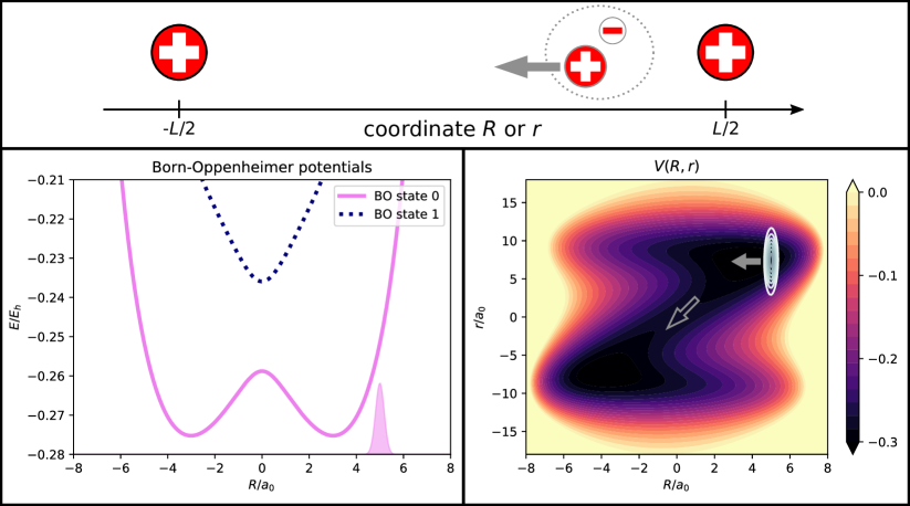
Figure 2: Top: A heavy particle with positive charge is positioned along coordinate $R$ and a light particle with negative charge is positioned along coordinate $r$, while two positive charges are clamped at $R=\pm L$, $r=\pm L$. The parameters of the model are chosen such that the positive charge gains momentum towards smaller $R$, dragging the negative charge along smaller $r$. Bottom left: The lowest two Born-Oppenheimer potentials for the heavy positive charge. Also shown is the initial marginal density of the positive charge. Bottom right: Model potential $V(R,r)$ and initial wavefunction for the dynamics. Two arrows indicate the motion during the dynamics.

A sketch of the model is depicted at the top of figure 2. A heavy positively charged particle can move along coordinate $R$ (the nucleus), and a light negatively charged particle can move along coordinate $r$ (the electron). Two clamped (infinitely heavy) positive charges are located at $(R,r)=(\pm L/2,\pm L/2)$. The model Hamiltonian is

$$H=-\frac{\mu}{2}\partial_{R}^{2}+\hat{H}_{\rm S}$$ (63)

with $\mu=m/M$ being the mass ratio between a light negatively charged particle (the electron) moving along dimension $r$ and a heavy positively charged particle (the nucleus) moving along dimension $R$, where

$$\hat{H}_{\rm S}=-\frac{\nabla_{\bm{r}}^{2}}{2}+V(R,r)$$ (64)

contains the kinetic energy of the light particle and the scalar interaction potential

$$V(R,r)=\frac{1}{|R-\frac{L}{2}|}+\frac{1}{|R+\frac{L}{2}|}-\frac{\operatorname{erf}\left(\frac{|r-R|}{R_{\rm c}}\right)}{|R-r|}-\frac{\operatorname{erf}\left(\frac{|r-\frac{L}{2}|}{R_{\rm r}}\right)}{|r-\frac{L}{2}|}-\frac{\operatorname{erf}\left(\frac{|r+\frac{L}{2}|}{R_{\rm l}}\right)}{|r+\frac{L}{2}|}.$$ (65)

We use the parameters $L=19$ $a_{0}$, $R_{\rm r}=R_{\rm l}=3.5$ $a_{0}$, $R_{\rm c}=4.0$ $a_{0}$, and a mass ratio $\mu^{-1}=900$. For these model parameters, the Born-Oppenheimer potential energy surfaces $\epsilon_{n}^{\rm BO}(R)$ for the nucleus, given by

$$\hat{H}_{\rm S}\phi_{n}^{\rm BO}(r|R)=\epsilon_{n}^{\rm BO}(R)\phi_{n}^{\rm BO}(r|R),$$ (66)

are energetically well-separated, as shown in the bottom-left panel of figure 2. The dynamics is adiabatic in the sense that

$$|\phi(r|R,t)|^{2}\approx|\phi_{0}^{\rm BO}(r|R)|^{2}$$ (67)

and the dynamics of the electron is parametrized by the configuration of the nucleus (the quantum clock) but only indirectly by the external time $t$.

The initial state for the dynamics is chosen to be a product of a Gaussian and the ground-state Born-Oppenheimer electronic wavefunction,

$$\psi_{0}(R,r)=\chi_{0}(R)\phi_{0}^{\rm BO}(r|R),$$ (68)

where

$$\chi_{0}(R)\propto e^{-\frac{(R-R_{0})^{2}}{4\sigma^{2}}}$$ (69)

with $R_{0}=5$ $a_{0}$ and $\sigma=0.183$ $a_{0}$. The density $|\chi_{0}(R)|^{2}$ is also shown in the bottom-left panel of figure 2. From the figure, it is clear that this wavepacket will initially move towards smaller $R$ and has enough energy to overcome the barrier at $R=0$. On the bottom-right panel of figure 2, the density $|\psi_{0}(R,r)|^{2}$ for the initial state is shown together with the potential $V(R,r)$ of (65). The dynamics is indicated by two arrows. For the chosen parameters it is essentially adiabatic in the sense of the Born-Oppenheimer approximation, i.e., the nucleus moves from its initial center at $R=5$ $a_{0}$ towards smaller $R$ and the electron follows from its initial center at ca. $r=8$ $a_{0}$ towards smaller $r$, resulting in the motion indicated by the arrows.

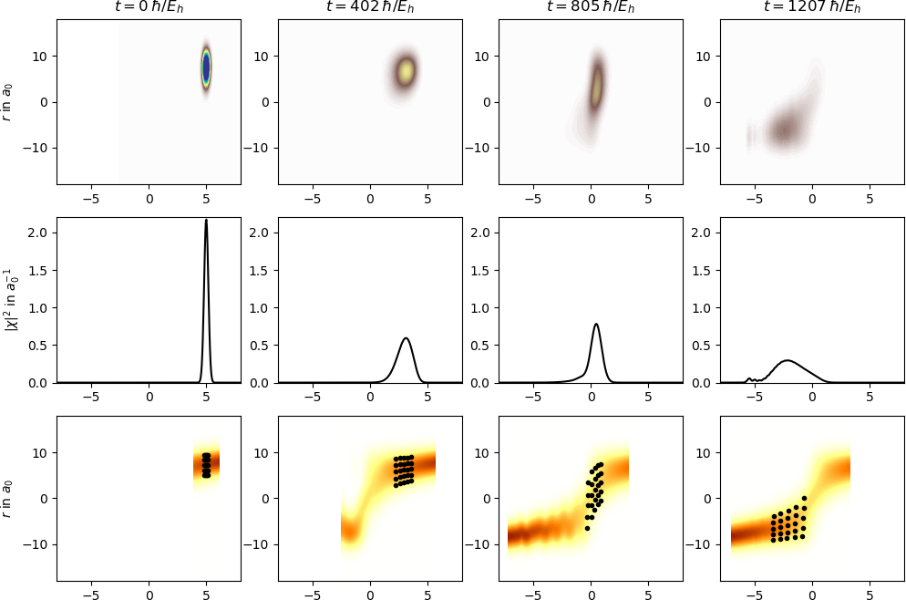
Figure 3: Density of the joint wavefunction $\psi(R,r|t)$ (top), of the marginal wavefunction $\chi(R|t)$ (middle), and of the conditional wavefunction $\phi(r|R,t)$ together with some of its corresponding trajectories (bottom) for four different values of the external time $t$.

Figure 3 shows the dynamics in terms of the joint probability density $|\psi(R,r|t)|^{2}$ (top), the marginal probability density of the nucleus $|\chi(R|t)|^{2}$ (center), and the conditional probability density of the electron $|\phi(r|R,t)|^{2}$ (bottom), for four different values of the external time $t$. The joint probability density follows the motion indicated by the arrows in figure 2, i.e., its maximum moves first towards smaller $R$, indicating the nuclear motion, but then also towards smaller $r$, indicating the electron following the nucleus. The motion towards smaller $R$ is clearly visible in the marginal nuclear density $|\chi(R|t)|^{2}$.

The probability density for our actual system of interest, the electron, is the conditional density $|\phi(r|R,t)|^{2}$ shown as contour plot in the bottom panels of figure 3. It is normalized for each value of $R$ (and $t$), hence it typically is somewhere localized along $r$ for every $R$. In the figure, $|\phi(r|R,t)|^{2}$ is only shown in a region of $R$ where the probability density of finding the nucleus is $|\chi(R|t)|^{2}>10^{-8}$ a${}_{0}^{-1}$, i.e., in a region where the clock can actually be found. Notwithstanding, there is no principle problem in obtaining $|\phi(r|R,t)|^{2}$ for all $R$, but there is a practical problem due to numerical inaccuracies whereever the joint probability density $|\psi(R,r|t)|^{2}$ becomes very small in magnitude.

Clock-dependent trajectories were computed for the wavefunction $\phi(r|R,t)$ using (61) and (62), where $\tau$ is identified with the external time $t$. The initial positions of the nucleus $R_{\rm t}(t=0)$ and of the electron $r_{\rm t}(t=0,R_{\rm t}(t=0))$ are chosen to be in a region where the density of the joint system $|\psi(R,r|t=0)|^{2}$ is significant. Then, (62) is solved to propagate the position of the nucleus $R_{\rm t}(t)$ along the trajectory. Thereafter, (61) is solved to propagate the electron $r_{\rm t}(t,R_{\rm t}(t))$ to the next value of $t$ and of $R_{\rm t}$, thus providing trajectories of the electron for each trajectory of the nucleus. The trajectories closely follow $|\phi(r|R,t)|^{2}$ with $t$, illustrating that these are indeed the conditional trajectories corresponding to the state of the electron, given the nucleus is at a certain position, and given a value for the external time $t$.

The considered dynamics is adiabatic in the sense of the Born-Oppenheimer approximation, which is typically interpreted as the electron following the nucleus “instantaneously”, staying in an eigenstate of $\hat{H}_{\rm S}$ given by (64). Thus, the probability density $|\phi(r|R,t)|^{2}$ is approximately the probability density of the Born-Oppenheimer wavefunction, cf. (67). The Born-Oppenheimer approximation, however, only provides an approximation to $|\phi(r|R,t)|$ but not to the phase of $\phi(r|R,t)$. Consequently, it does not provide the electronic flux density and hence not the electronic motion.barth2009 ; scherrer2013 ; schild2016 However, the dynamics is also adiabatic for the phase of $\phi(r|R,t)$, not only for its magnitude: Instead of solving the Born-Oppenheimer TISE (66), the CDSE (31) can be solved with the nucleus being the clock but without explicit reference to the external time $t$. As explained in schild2018 , solving such a CDSE (the term $\hat{U}\phi$ and a term $\partial_{t}\phi$ that appears in a time- and clock-dependent treatment can be neglected) provides an excellent approximation to $\phi(r|R,t)$.

As illustrated in schild2018 with the clock-dependent continuity equation and as can be expected from the idea of the Born-Oppenheimer approximation, the relevant clock for the electron in the adiabatic limit is the nucleus, while $t$ is only affecting the dynamics indirectly as parameter for the trajectory of the nucleus. Thus, each of the trajectories $r_{\rm t}(t,R_{\rm t}(t))$ can be read as $r_{\rm t}(R_{\rm t})$, where $R_{\rm t}$ provides a possible trajectory of the clock. It is in this sense that the model illustrates trajectories obtained from the CDSE, even though the overall dynamics within the model is generated by solving a TDSE for the joint system.

VI Discussion

The CDSE (31) is the generalization of the TDSE (1) in case changes in a quantum system are compared to a clock which is treated quantum-mechanically, i.e., which is described by a wavefunction. Such a clock does not provide a single time parameter via a well-defined (classical) position and velocity. Notwithstanding, the CDSE (like the TDSE) represents the conditional dependence of the quantum system on the configuration of the clock, hence there is no uncertainty of the clock configuration in the CDSE like there is no uncertainty of time in the TDSE. The “quantum” effect of the clock is that different paths trough the space of the clock configurations are possible.

The CDSE can be used in a way that is very similar to the TDSE. In this article, the CDSE is used to derive the clock-dependent analogue of time-dependent quantum hydrodynamics. A clock-dependent Hamilton-Jacobi equation as well as a clock-dependent continuity equation are obtained which are similar to their time-dependent counterparts, but which contain additional terms. In particular, in the clock-dependent versions of the equations the spatial variation of the probability density of the clock is relevant.

The method of characteristics can be used to solve the clock-dependent Hamilton-Jacobi equation, thus providing clock-dependent quantum trajectories. Specifically, trajectories for the clock are obtained, which depend on an arbitrary parameter $\tau$, as well as trajectories for the actual system of interest, which depend on the configuration of the clock. The existence of these trajectories is interesting in itself, as is the parameter $\tau$ which comes from the way how the differential equation is solved but which works very much like a normal time parameter: It parametrizes the trajectory of the clock, which in turn parametrizes the trajectory of the system.

The model presented in section V illustrates that clock-dependent quantum trajectories may be a useful computational tool. For example, there is the problem of computing electron dynamics in molecular systems interacting with strong laser fields. Laser pulses of attosecond duration are available to probe such electron dynamics, which lead to the development of novel theoretical tools to simulate the complicated laser-induced dynamics of molecules on this time scale.palacios2019 Especially for larger molecules, those rely on a clamped-nuclei approximation of on trajectory simulations for the nuclear wavefunction.robb2018 ; mai2018 ; agostini2018book ; mignolet2019 ; penfold2019 ; palacios2019 Additionally, many effects occurring in strong laser fields can be described qualitatively with the help of simple trajectory calculations for the electrons. lewenstein1994 ; salieres2001 ; takemoto2011 The clock-dependent quantum trajectory formalism may provide the starting point for developing simulations methods that treat both nuclei and electrons in a trajectory-based picture, thus allowing to include necessary quantum effects on all levels. A branching of the nuclear wavepacket, for example, can be described with a set of trajectories for the nuclei (the clock) that give rise to a set of trajectories for the electrons. For this purpose, next to (61) and (62) also equations for the momenta need to be solved, which can be expected to pose similar challenges like time-dependent quantum trajectories wyatt2005 . The discussion of these equations is, however, beyond the scope of this paper. Nevertheless, we note that for the considered model, (62) can be simplified by neglecting the momentum field associated with the electronic wavefunction $\phi$, thus simplifying a possible propagation of the trajectories without previous knowledge of the wavefunctions.

Notwithstanding these possible practical applications of the formalism, there are conceptual challenges. Next to the obvious limitation that this article is only concerned with non-relativistic quantum mechanics, a central open question is: Where does the dynamics come from? According to the formalism presented here, the differential equation for the trajectory of the clock (62) shows that the momentum field $\bm{P}_{\rm t}[\psi]$ generates changes of the clock configuration. If the wavefunction $\psi$ of the super-system, composed of the clock and the quantum system of interest, is generated by solving a TDSE with some initial conditions, there is a dynamics due to the “passing” of an unspecified external time parameter. This is the case for the presented proton-coupled electron transfer model, where an external time parameter was assumed. In contrast, for a truly closed system without reference to anything external, we expect $\psi$ to be an eigenstate of the Hamiltonian and thus been given by a TISE. Then, $\bm{P}_{\rm t}[\psi]$ is zero if $\psi$ is real-valued. For $\bm{P}_{\rm t}[\psi]$ to be non-zero, and thus for a dynamics to happen at all, $\psi$ needs e.g. to correspond to some rotating state, suitable boundary conditions need to be imposed, or other modifications to the formalism need to be made. It is thus not trivial to invent a model for purely clock-dependent quantum mechanics, without reference to an external time, that shows a dynamics.

The question about the “origin of dynamics” may be related to the ignorance of relativistic effects, to the missing mechanism for deciding which path the clock actually takes (i.e., the measurement or how internal observers can be described), to the assumption of an absolute space (time is defined relative to a clock, but space was assumed to be absolute in this article), or to something completely different. It will be interesting to see if and how this question can be solved.

Acknowledgment

This research is supported by an Ambizione grant of the Swiss National Science Foundation.

References

- (1) C. J. Isham. Canonical Quantum Gravity and the Problem of Time. In L. A. Ibort and M. A. Rodríguez, editors, Integrable Systems, Quantum Groups, and Quantum Field Theory, page 157. Kluwer Academic Publishers, 1993.
- (2) Edward Anderson. The Problem of Time. Spinger International Publishing AG, Cham, Switzerland, 2017.
- (3) Sougato Bose, Anupam Mazumdar, Gavin W. Morley, Hendrik Ulbricht, Marko Toroš, Mauro Paternostro, Andrew A. Geraci, Peter F. Barker, M. S. Kim, and Gerard Milburn. Spin entanglement witness for quantum gravity. Phys. Rev. Lett., 119:240401, Dec 2017.
- (4) Daniel Carney, Philip C E Stamp, and Jacob M Taylor. Tabletop experiments for quantum gravity: a user’s manual. Classical and Quantum Gravity, 36(3):034001, 2019.
- (5) John Preskill. Quantum Computing in the NISQ era and beyond. Quantum, 2:79, 2018.
- (6) Daniela Frauchiger and Renato Renner. Quantum theory cannot consistently describe the use of itself. Nat. Commun., 9:3711, 2018.
- (7) D. Lazarovici and M. Hubert. How Quantum Mechanics can consistently describe the use of itself. Sci. Rep., 9:470, 2019.
- (8) Daniel F. Styer, Miranda S. Balkin, Kathryn M. Becker, Matthew R. Burns, Christopher E. Dudley, Scott T. Forth, Jeremy S. Gaumer, Mark A. Kramer, David C. Oertel, Leonard H. Park, Marie T. Rinkoski, Clait T. Smith, and Timothy D. Wotherspoon. Nine formulations of quantum mechanics. American Journal of Physics, 70(3):288–297, 2002.
- (9) E. Madelung. Eine anschauliche Deutung der Gleichung von Schrödinger. Naturwissenschaften, 14:1004, 1926.
- (10) E. Madelung. Quantentheorie in hydrodynamischer Form. Zeitschrift für Physik, 40:322, 1927.
- (11) de Broglie, Louis. La mécanique ondulatoire et la structure atomique de la matière et du rayonnement. J. Phys. Radium, 8(5):225–241, 1927.
- (12) David Bohm. A Suggested Interpretation of the Quantum Theory in Terms of ”Hidden” Variables. I. Phys. Rev., 85:166–179, Jan 1952.
- (13) David Bohm. A Suggested Interpretation of the Quantum Theory in Terms of ”Hidden” Variables. II. Phys. Rev., 85:180–193, Jan 1952.
- (14) John Bell. Against ‘measurement’. Physics World, 3(8):33–41, aug 1990.
- (15) Timothy J. Hollowood. Copenhagen quantum mechanics. Contemporary Physics, 57(3):289–308, 2016.
- (16) K. Landsman. Foundations of Quantum Theory, chapter The measurement problem, page 435. Springer, Cham, Switzerland, 2017.
- (17) Aephraim M. Steinberg. How much time does a tunneling particle spend in the barrier region? Phys. Rev. Lett., 74:2405–2409, Mar 1995.
- (18) Alexandra S. Landsman and Ursula Keller. Attosecond science and the tunnelling time problem. Physics Reports, 547:1, 2015.
- (19) Tomá š Zimmermann, Siddhartha Mishra, Brent R. Doran, Daniel F. Gordon, and Alexandra S. Landsman. Tunneling time and weak measurement in strong field ionization. Phys. Rev. Lett., 116:233603, Jun 2016.
- (20) D. Sokolovski and E. Akhmatskaya. No time at the end of the tunnel. Communications Physics, 1:47, 2018.
- (21) Makoto Tsubota, Michikazu Kobayashi, and Hiromitsu Takeuchi. Quantum hydrodynamics. Physics Reports, 522(3):191 – 238, 2013.
- (22) P. K. Shukla and B. Eliasson. Colloquium: Nonlinear collective interactions in quantum plasmas with degenerate electron fluids. Rev. Mod. Phys., 83:885–906, Sep 2011.
- (23) Zh. A. Moldabekov, M. Bonitz, and T. S. Ramazanov. Theoretical foundations of quantum hydrodynamics for plasmas. Physics of Plasmas, 25(3):031903, 2018.
- (24) Ingo Barth and Klaus Renziehausen. Many-particle quantum hydrodynamics: Exact equations and pressure tensors. Progress of Theoretical and Experimental Physics, 2018(1), 01 2018.
- (25) Detlef Dürr, Sheldon Goldstein, and Nino Zanghí. Quantum equilibrium and the origin of absolute uncertainty. Journal of Statistical Physics, 67:843–907, 1992.
- (26) Detlef Dürr, Sheldon Goldstein, and Nino Zanghì. Quantum equilibrium and the role of operators as observables in quantum theory. Journal of Statistical Physics, 116:959–1055, 2004.
- (27) Travis Norsen. Bohmian conditional wave functions (and the status of the quantum state). Journal of Physics: Conference Series, 701:012003, 2016.
- (28) Robert E. Wyatt, Courtney L. Lopreore, and Gérard Parlant. Electronic transitions with quantum trajectories. The Journal of Chemical Physics, 114(12):5113–5116, 2001.
- (29) Courtney L. Lopreore and Robert E. Wyatt. Electronic transitions with quantum trajectories. ii. The Journal of Chemical Physics, 116(4):1228–1238, 2002.
- (30) Robert E. Wyatt. Quantum Dynamics with Trajectories – Introduction to Quantum Hydrodynamics. Springer, 2005.
- (31) Vitaly A. Rassolov and Sophya Garashchuk. Semiclassical nonadiabatic dynamics with quantum trajectories. Phys. Rev. A, 71:032511, Mar 2005.
- (32) Basile F. E. Curchod and Ivano Tavernelli. On trajectory-based nonadiabatic dynamics: Bohmian dynamics versus trajectory surface hopping. The Journal of Chemical Physics, 138(18):184112, 2013.
- (33) Federica Agostini, Ivano Tavernelli, and Giovanni Ciccotti. Nuclear quantum effects in electronic (non)adiabatic dynamics. The European Physical Journal B, 91(7):139, 2018.
- (34) Yair Goldfarb, Ilan Degani, and David J. Tannor. Bohmian mechanics with complex action: A new trajectory-based formulation of quantum mechanics. The Journal of Chemical Physics, 125(23):231103, 2006.
- (35) Noa Zamstein and David J. Tannor. Non-adiabatic molecular dynamics with complex quantum trajectories. I. The diabatic representation. The Journal of Chemical Physics, 137(22):22A517, 2012.
- (36) Noa Zamstein and David J. Tannor. Non-adiabatic molecular dynamics with complex quantum trajectories. ii. the adiabatic representation. The Journal of Chemical Physics, 137(22):22A518, 2012.
- (37) Werner Koch and David J. Tannor. Wavepacket revivals via complex trajectory propagation. Chemical Physics Letters, 683:306 – 314, 2017. Ahmed Zewail (1946-2016) Commemoration Issue of Chemical Physics Letters.
- (38) X. Oriols. Quantum-trajectory approach to time-dependent transport in mesoscopic systems with electron-electron interactions. Phys. Rev. Lett., 98:066803, Feb 2007.
- (39) Albert Benseny, Guillermo Albareda, Ángel S. Sanz, Jordi Mompart, and Xavier Oriols. Applied bohmian mechanics. Eur. Phys. J. D, 68:286, 2014.
- (40) Guillermo Albareda, Heiko Appel, Ignacio Franco, Ali Abedi, and Angel Rubio. Correlated electron-nuclear dynamics with conditional wave functions. Phys. Rev. Lett., 113:083003, Aug 2014.
- (41) Guillermo Albareda, Damiano Marian, Abdelilah Benali, Alfonso Alarcón, Simeon Moises, and Xavier Oriols. Electron Devices Simulation with Bohmian Trajectories, chapter 7, pages 261–318. Wiley-Blackwell, 2016.
- (42) Don N. Page and William K. Wootters. Evolution without evolution: Dynamics described by stationary observables. Phys. Rev. D, 27:2885–2892, Jun 1983.
- (43) William K. Wootters. “Time” Replaced by Quantum Correlations. International Journal of Theoretical Physics, 23:701, 1984.
- (44) Ekaterina Moreva, Giorgio Brida, Marco Gramegna, Vittorio Giovannetti, Lorenzo Maccone, and Marco Genovese. Time from quantum entanglement: An experimental illustration. Phys. Rev. A, 89:052122, May 2014.
- (45) E. Moreva, G. Brida, M. Gramegna, V. Giovannetti, L. Maccone, and M. Genovese. The time as an emergent property of quantum mechanics, a synthetic description of a first experimental approach. Journal of Physics: Conference Series, 626(1):012019, 2015.
- (46) Vittorio Giovannetti, Seth Lloyd, and Lorenzo Maccone. Quantum time. Phys. Rev. D, 92:045033, Aug 2015.
- (47) Ekaterina Moreva, Marco Gramegna, Giorgio Brida, Lorenzo Maccone, and Marco Genovese. Quantum time: Experimental multitime correlations. Phys. Rev. D, 96:102005, Nov 2017.
- (48) C. Marletto and V. Vedral. Evolution without evolution and without ambiguities. Phys. Rev. D, 95:043510, Feb 2017.
- (49) K. L. H. Bryan and A. J. M. Medved. Realistic clocks for a universe without time. Foundations of Physics, 48:48, 2018.
- (50) Alexander R. H. Smith and Mehdi Ahmadi. Quantizing time: Interacting clocks and systems. Quantum, 3:160, 2019.
- (51) T. Banks. , quantum gravity, the cosmological constant and all that…. Nuclear Physics B, 249:332, 1985.
- (52) R. Brout. On the Concept of Time and the Origin of the Cosmological Temperature. Foundations of Physics, 17:603, 1987.
- (53) F. Englert. Quantum physics without time. Physics Letters B, 228:111, 1989.
- (54) J. S. Briggs and J. M. Rost. Time dependence in quantum mechanics. The European Physical Journal D, 10:311, 2000.
- (55) Julian Barbour, Tim Koslowski, and Flavio Mercati. The solution to the problem of time in shape dynamics. Class. Quantum Grav., 31:155001, 2014.
- (56) Julian Barbour, Tim Koslowski, and Flavio Mercati. Identification of a gravitational arrow of time. Phys. Rev. Lett., 113:181101, Oct 2014.
- (57) Lars Braun, Walter T. Strunz, and John S. Briggs. Classical limit of the interaction of a quantum system with the electromagnetic field. Phys. Rev. A, 70:033814, Sep 2004.
- (58) John S. Briggs and James M. Feagin. Scattering theory, multiparticle detection, and time. Phys. Rev. A, 90:052712, Nov 2014.
- (59) John S. Briggs. Equivalent emergence of time dependence in classical and quantum mechanics. Phys. Rev. A, 91:052119, May 2015.
- (60) Axel Schild. Time in quantum mechanics: A fresh look at the continuity equation. Phys. Rev. A, 98:052113, Nov 2018.
- (61) Ali Abedi, Neepa T. Maitra, and E. K. U. Gross. Exact factorization of the time-dependent electron-nuclear wave function. Phys. Rev. Lett., 105:123002, Sep 2010.
- (62) Ali Abedi, Neepa T. Maitra, and E. K. U. Gross. Correlated electron-nuclear dynamics: Exact factorization of the molecular wavefunction. The Journal of Chemical Physics, 137(22):22A530, 2012.
- (63) M. Born and R. Oppenheimer. Zur quantentheorie der molekeln. Annalen der Physik, 389(20):457–484, 1927.
- (64) U. Klein. What is the limit of quantum theory? American Journal of Physics, 80(11):1009–1016, 2012.
- (65) F. G. Eich and Federica Agostini. The adiabatic limit of the exact factorization of the electron-nuclear wave function. The Journal of Chemical Physics, 145(5):054110, 2016.
- (66) Sophya Garashchuk, David Dell’Angelo, and Vitaly A. Rassolov. Dynamics in the quantum/classical limit based on selective use of the quantum potential. The Journal of Chemical Physics, 141(23):234107, 2014.
- (67) Xing Gao and Walter Thiel. Non-hermitian surface hopping. Phys. Rev. E, 95:013308, Jan 2017.
- (68) Rutherford Aris. Vectors, Tensors, and the Basic Equations of Fluid Mechanics. Dover, New York, 1989.
- (69) Geoffrey Hunter. Conditional probability amplitudes in wave mechanics. International Journal of Quantum Chemistry, 9(2):237–242, 1975.
- (70) Ingo Barth, Hans-Christian Hege, Hiroshi Ikeda, Anatole Kenfack, Michael Koppitz, Jörn Manz, Falko Marquardt, and Guennaddi K. Paramonov. Concerted quantum effects of electronic and nuclear fluxes in molecules. Chemical Physics Letters, 481(1):118 – 123, 2009.
- (71) A. Scherrer, R. Vuilleumier, and D. Sebastiani. Nuclear velocity perturbation theory of vibrational circular dichroism. Journal of Chemical Theory and Computation, 9(12):5305–5312, 2013. PMID: 26592268.
- (72) Axel Schild, Federica Agostini, and E. K. U. Gross. Electronic Flux Density beyond the Born-Oppenheimer Approximation. The Journal of Physical Chemistry A, 120(19):3316–3325, 2016. PMID: 26878256.
- (73) Alicia Palacios and Fernando Martín. The quantum chemistry of attosecond molecular science. WIREs Computational Molecular Science, n/a(n/a):e1430, 2019.
- (74) Michael A. Robb, Andrew J. Jenkins, and Morgane Vacher. How nuclear motion affects coherent electron dynamics in molecules. In Marc J. J. Vrakking and Franck Lepine, editors, Attosecond Molecular Dynamics, pages 275–307. The Royal Society of Chemistry, 2018.
- (75) Sebastian Mai, Felix Plasser, Philipp Marquetand, and Leticia González. General trajectory surface hopping method for ultrafast nonadiabatic dynamics. In Marc J. J. Vrakking and Franck Lepine, editors, Attosecond Molecular Dynamics, pages 348–385. The Royal Society of Chemistry, 2018.
- (76) Federica Agostini, Basile F. E. Curchod, Rodolphe Vuilleumier, Ivano Tavernelli, and E. K. U. Gross. Tddft and quantum-classical dynamics: A universal tool describing the dynamics of matter. In Wanda Andreoni and Sidney Yip, editors, Handbook of Materials Modeling: Methods: Theory and Modeling, pages 1–47. Springer International Publishing, Cham, 2018.
- (77) Benoit Mignolet and Basile F. E. Curchod. Excited-state molecular dynamics triggered by light pulses—ab initio multiple spawning vs trajectory surface hopping. The Journal of Physical Chemistry A, 123(16):3582–3591, 2019. PMID: 30938525.
- (78) T.J. Penfold, M. Pápai, K.B. Møller, and G.A. Worth. Excited state dynamics initiated by an electromagnetic field within the Variational Multi-Configurational Gaussian (vMCG) method. Computational and Theoretical Chemistry, 1160:24 – 30, 2019.
- (79) M. Lewenstein, Ph. Balcou, M. Yu. Ivanov, Anne L’Huillier, and P. B. Corkum. Theory of high-harmonic generation by low-frequency laser fields. Phys. Rev. A, 49:2117–2132, Mar 1994.
- (80) P. Salières, B. Carré, L. Le Déroff, F. Grasbon, G. G. Paulus, H. Walther, R. Kopold, W. Becker, D. B. Milošević, A. Sanpera, and M. Lewenstein. Feynman’s path-integral approach for intense-laser-atom interactions. Science, 292(5518):902–905, 2001.
- (81) Norio Takemoto and Andreas Becker. Visualization and interpretation of attosecond electron dynamics in laser-driven hydrogen molecular ion using bohmian trajectories. The Journal of Chemical Physics, 134(7):074309, 2011.