The detection of dust gap-ring structure in the outer region of the CR Cha protoplanetary disk

Abstract

We observe the dust continuum at 225 GHz and CO isotopologue (¹²CO, ¹³CO, and C¹⁸O) $J=2-1$ emission lines toward the CR Cha protoplanetary disk using the Atacama Large Millimeter/submillimeter Array (ALMA). The dust continuum image shows a dust gap-ring structure in the outer region of the dust disk. A faint dust ring is also detected around 120 au beyond the dust gap. The CO isotopologue lines indicate that the gas disk is more extended than the dust disk. The peak brightness temperature of the ¹³CO line shows a small bump around 130 au while ¹²CO and C¹⁸O lines do not show. We investigate two possible mechanisms for reproducing the observed dust gap-ring structure and a gas temperature bump. First, the observed gap structure can be opened by a Jupiter mass planet using the relation between the planet mass and the gap depth and width. Meanwhile, the radiative transfer calculations based on the observed dust surface density profile show that the observed dust ring could be formed by dust accumulation at the gas temperature bump, that is, the gas pressure bump produced beyond the outer edge of the dust disk.

1 Introduction

CR Cha (a.k.a Sz 6, Cha T8) is a K-type pre-main sequence star (Hussain et al., 2009; Villebrun et al., 2019) in Cha I dark cloud, one of the famous star forming clouds in our galaxy.  The fitting on the stellar evolution tracks suggests that the stellar mass of CR Cha is $M_{\star}=1.2-2\rm~{}M_{\odot}$ with an age of $1-3$ Myr (e.g., D’Antona & Mazzitelli, 1994; Natta et al., 2000; Hussain et al., 2009; Varga et al., 2018). The latest updated distance of CR Cha is $d\sim 187.5\pm 0.8\rm~{}pc$ (GAIA DR 2; Gaia Collaboration et al., 2018). The existence of the protoplanetary disk around CR Cha had already been revealed by the thermal dust emission at (sub-)mm wavelengths (e.g., Ubach et al., 2012; Pascucci et al., 2016; Ribas et al., 2017; Ubach et al., 2017).

The spectral index $\alpha$ at mm-wavelength is linked to the dust properties, such as dust opacity and the dust grain size (e.g., Miyake & Nakagawa, 1993). It can be used to study the dust growth in the disk by comparing with the spectral index of the interstellar medium (ISM) (e.g., Beckwith & Sargent, 1991; D’Alessio et al., 2001).  Toward the CR Cha disk, the measured spectral index at 1 mm is $\alpha_{\rm 1mm}\sim 3.4$ (Ubach et al., 2012), which is close to $\alpha_{\rm ISM}\sim 3.7$ in the ISM.  This large $\alpha_{\rm 1mm}$ value in the CR Cha disk indicates that the maximum grain size is small in the outer disk (e.g., Draine, 2006). This may be the results of the dust growth in this region: the mm-sized dust grains already drifted inward in the gas disk due to the gas drag (Ribas et al., 2017; Ubach et al., 2017). Recent CO line survey toward the protoplanetary disks in Cha I cloud using Atacama Large Millimeter/submillimeter Array (ALMA) can support this possibility by detecting that the gas disk around the CR Cha exists with an angular size of $\sim 0.9^{\prime\prime}$ in radius (Long et al., 2017).

However, the time scale of the radial drift of mm/cm-sized dust grains ($10^{4-5}$ yr; e.g., Takeuchi & Lin, 2005; Brauer et al., 2007) is much shorter than the age of CR Cha ($\sim 1-3~{}\rm Myr$). Ribas et al. (2017) suggested that some braking mechanisms, such as dust trapping at the pressure bumps produced by zonal flow (e.g., Pinilla et al., 2012) or a planet-opened gaps (e.g., Zhu et al., 2012), are required to stop or slow down the radial drift of the dust grains. That is, the CR Cha disk is one of the strong candidates which would have disk substructures like a dust ring/gap.

In this paper, we show the results of the dust continuum and the CO isotopologue $J=2-1$ emission lines observed at ALMA Band 6 to examine the existence of small scale disk substructure like a gap or ring structure in the CR Cha disk. We summarize the information of ALMA observations toward the CR Cha disk in Section 2. The observed dust continuum and CO isotopologue images are presented in Section 3. In Section 4, we discuss the radial profiles of dust surface density and CO gas column density derived from the observations and the possible mechanisms to explain the detected CR Cha disk structure. Finally, we summarize our results in Section 5.

Table 1: The summary of dust continuum and CO isotopologue line images.

Species	$\nu_{\rm center}$	RMS in Cube	RMS in Mom. 0	Beam size	Beam PA
	[GHz]	[mJy beam-1]	[mJy beam-1 km s-1]	[arcsec2]	[∘]
Dust	225	$\sim 0.0178$		$0.087\times 0.052$	35.75
12CO	230.538	$\sim 2.47$	$\sim$4.594	$0.188\times 0.128$	0.635
13CO	220.398	$\sim 2.40$	$\sim$4.978	$0.196\times 0.143$	0.405
C18O	219.560	$\sim 2.28$	$\sim$3.441	$0.194\times 0.142$	0.976

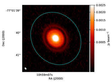
(a) Dust continuum at 225 GHz

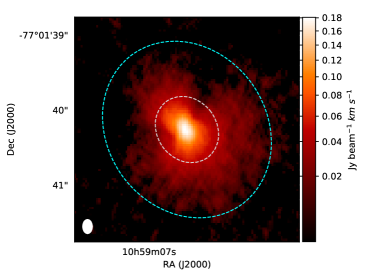
(b) ¹²CO emission line

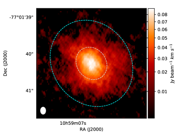
(c) ¹³CO emission line

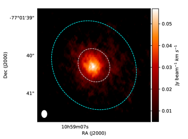
(d) C¹⁸O emission line

Figure 1: (a) The 225 GHz dust continuum image and the moment 0 maps of (b) ¹²CO, (c) ¹³CO, and (d) C¹⁸O $J=2-1$ line emission of the CR Cha disk. The synthesized beam is presented in the bottom-left corner: $\sim 0.087^{\prime\prime}\times 0.052^{\prime\prime}$ for the dust continuum emission (Briggs robust=0), $\sim 0.188^{\prime\prime}\times 0.128^{\prime\prime}$ for ¹²CO, $\sim 0.196^{\prime\prime}\times 0.143^{\prime\prime}$ for ¹³CO, and $\sim 0.194^{\prime\prime}\times 0.142^{\prime\prime}$ for C¹⁸O line emission (Briggs robust=2). The colorbar indicates the observed intensity in $\rm Jy~{}beam^{-1}$ unit for the dust continuum and the integrated intensities in $\rm Jy~{}beam^{-1}~{}km~{}s^{-1}$ unit for the CO isotopologue lines. The white dashed ellipse shows the location of the dust gap at $\rm r=90~{}au$. A faint dust ring is detected beyond the dust gap. The cyan dashed ellipse indicates the outer edge of the CO gas disks at $\rm r=240~{}au$.

2 Observation

The CR Cha protoplanetary disk is observed at ALMA Band 6 on November 2017 and March 2018 with 47 and 42 antennae respectively (2017.1.00286.S). The projected baselines are from 12.54 m to 7.908 km, corresponding to a maximum angular coverage of $\sim 5^{\prime\prime}$ and an angular resolution of $\gtrsim 0.06^{\prime\prime}$. The total execution time for the observations is $\sim 3.2$ hours including the target on-source time of $\sim 2$ hours. J1427-4206 and J0635-7516 are used for the bandpass and flux calibrations at each observation. J1058-8003 is selected as a phase calibrator at both observations.

The correlator setup has four spectral windows (SPWs). Dust continuum emission is observed at 233 GHz (SPW1) and 217 GHz (SPW2) with 1.8 GHz bandwidth at each SPW. For the CO isotopologue emission lines, the SPWs are centered at 230.538 GHz for ¹²CO (SPW0), 220.398 GHz for ¹³CO, and 219.560 GHz for C¹⁸O (SPW3). The spectral resolution for three CO isotopologue lines is 61 kHz, corresponding to $\rm\sim 0.08~{}km~{}s^{-1}$ in velocity.

The basic calibration steps are progressed through the ALMA calibration pipeline using CASA package version 5.3. After the ALMA pipeline calibration, we make the images of dust continuum and CO isotopologue emission lines by CLEAN command in CASA. The Briggs $\rm robust=0$ is used for the dust continuum image, obtaining the synthesized beam size of $\sim 0.087^{\prime\prime}\times 0.052^{\prime\prime}$ and the beam position angle (PA) of $\sim 35.75^{\circ}$. The phase self-calibration is applied to the dust continuum image for improving the data quality. Meanwhile, the Briggs $\rm robust=2.0$ (Natural weighting) is applied for the CO isotopologue lines to obtain high signal-to-noise ratio $\rm(SNR)\sim 20-30$. We also apply the phase self-calibration to the CO line data but the images are not improved. We note that the SNRs of the CO isotopologue lines are $\sim 5-7$ with $\sim 0.080^{\prime\prime}\times 0.047^{\prime\prime}$ synthesized beam size when the $\rm robust=0$ is applied. The synthesized beam size is $\sim 0.188^{\prime\prime}\times 0.128^{\prime\prime}$ for the ¹²CO line, $\sim 0.196^{\prime\prime}\times 0.143^{\prime\prime}$ for the ¹³CO line, and $\sim 0.194^{\prime\prime}\times 0.142^{\prime\prime}$ for C¹⁸O line, respectively. Table 1 summarizes the angular resolution and RMS noise level of the observed data.

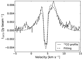
(a) ¹²CO spectrum

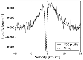
(b) ¹³CO spectrum

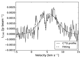
(c) C¹⁸O spectrum

Figure 2: The averaged spectra (solid line) of (a) ¹²CO, (b) ¹³CO, and (c) C¹⁸O $J=2-1$ emission lines inside the disk radius of $\rm r\lesssim 240$ au. The dashed lines are the Gaussian fitting of the emission plus absorption profiles. The emission lines are centered at $\rm\sim 5.3~{}km~{}s^{-1}$ with $\Delta V_{\rm emis}$ of $\rm\sim 2.7~{}km~{}s^{-1}$ on average. The absorption features are centered at $\rm\sim 4.5~{}km~{}s^{-1}$ with $\Delta V_{\rm abs}$ of $\rm\sim 0.2-0.5~{}km~{}s^{-1}$. The fitting parameters are summarized in Table 2.

Table 2: The summary of Gaussian fitting parameters for the emission and absorption of the CO isotopologue lines.

Species	$A_{\rm emis}$	$V_{\rm emis}$	$\Delta V_{\rm emis}$	$A_{\rm abs}$	$V_{\rm abs}$	$\Delta V_{\rm abs}$
	[mJy beam-1]	[km s-1]	[km s-1]	[mJy beam-1]	[km s-1]	[km s-1]
12CO	6.37$\pm$0.22	5.30$\pm$0.07	2.67$\pm$0.07	-10.26$\pm$0.34	4.46$\pm$0.02	0.52$\pm$0.02
13CO	5.00$\pm$0.11	5.19$\pm$0.06	2.64$\pm$0.06	-9.97$\pm$0.30	4.50$\pm$0.01	0.25$\pm$0.01
C18O	1.90$\pm$0.08	5.51$\pm$0.13	2.96$\pm$0.13	-1.24$\pm$0.26	4.56$\pm$0.05	0.21$\pm$0.05

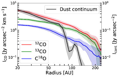
(a) The azimuthally averaged (integrated) intensity profiles

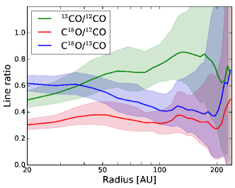
(b) The ratios between the CO isotopologue lines

Figure 3: (a) The azimuthally averaged radial profiles of the dust continuum emission (black) in $\rm Jy~{}arcsec^{-2}$ unit and the integrated intensities of ¹²CO (red), ¹³CO (green), and C¹⁸O (blue) emission lines in $\rm Jy~{}arcsec^{-2}~{}km~{}s^{-1}$ unit. The color-shaded regions indicate the uncertainty due to the azimuthal average. The dust continuum emission shows a gap at $\sim 90$ au and a ring at $\sim 120$ au. Meanwhile, the CO isotopologue emissions extend to $\rm r\sim 240$ au smoothly. (b) The ratios between the azimuthally averaged integrated intensity profiles of the CO isotopologue lines: ¹³CO/¹²CO (green), C¹⁸O/¹²CO (red), and C¹⁸O/¹³CO (blue). The color-shaded regions show the uncertainty due to those of azimuthally averaged integrated CO intensity profiles.

3 Result

3.1 The images of dust continuum and CO isotopologue emission lines

Figure 1(a) shows the dust continuum image at 225 GHz. There is a dust gap at $\rm r\sim 90$ au and a faint dust ring just beyond the dust gap. The total flux density of the dust disk is $\sim 0.139$ Jy. It is consistent with the previous observation of $F\sim 0.125$ Jy at 1.2 mm continuum (Ubach et al., 2012). The $1\sigma$ RMS level of dust continuum image is $\rm\sim 0.0178~{}mJy~{}beam^{-1}$. The peak intensity of the dust ring is $\sim 10\sigma$ RMS level on average. We obtain the disk geometry by the ellipse fitting using imfit command in CASA package. The estimated inclination of the disk is $31.0^{\circ}\pm 1.4^{\circ}$ and disk PA is $36.2^{\circ}\pm 1.8^{\circ}$.

Figure 1(b), (c), and (d) show the integrated intensity maps (moment 0 maps) of the continuum subtracted line emissions of ¹²CO, ¹³CO, and C¹⁸O, respectively. The white dashed ellipse presents the annulus at $\rm r=90~{}au$ which is corresponding to the dust gap in Figure 1(a). The cyan dashed ellipse indicates the outer edge of the CO gas disk at $\rm r=240~{}au$. This radius corresponds to the detection limit of the CO isotopologue lines, where the peak intensity at each pixel (the moment 8 map; Figure 4(a) and (b)) is $\rm\sim 7.5~{}mJy~{}beam^{-1}$, $\approx 3\sigma$ RMS level of the data cubes of the CO isotopologue lines. They show that the gas disk of CR Cha is much extended than the dust disk.

The solid lines in Figure 2 present the averaged spectra of (a) ¹²CO, (b) ¹³CO, and (c) C¹⁸O line emission inside the disk radius of $\rm r\lesssim 240$ au, applying the disk inclination of $31^{\circ}$ and the disk PA of $36.2^{\circ}$. There is a strong absorption feature at the velocity of $\sim 4.5$ km s^-1 in the ¹²CO and ¹³CO spectra. The absorption feature in C¹⁸O line spectrum is less prominent than those of ¹²CO and ¹³CO. This absorption feature is also well seen in the channel maps (see Appendix A) and the moment 8 maps of ¹²CO and ¹³CO lines (see Figure 4(a) and (b)).

We perform the least mean square fitting for the emission and absorption lines to measure their strengths, velocity centers, and width. We use the following function for the fitting:

$$\begin{split}{\rm I}_{\nu}=&A_{\rm emit}\exp\left(-\frac{\left(V-V_{\rm emis}\right)^{2}}{2\Delta V_{\rm emis}^{2}}\right)\\ &+A_{\rm abs}\exp\left(-\frac{\left(V-V_{\rm abs}\right)^{2}}{2\Delta V_{\rm abs}^{2}}\right).\end{split}$$ (1)

The fitting parameters are summarized in Table 2. The dashed lines in Figure 2 show the fitting results of the emission plus absorption profiles. The fitting results show that the CO emission lines are centered at $\sim 5.3$ km s^-1 with $\Delta V_{\rm emis}$ of $\sim 2.7$ km s^-1 on average and the absorption feature is centered at $\sim 4.5$ km s^-1 with $\Delta V_{\rm abs}$ of $\sim 0.2-0.5$ km s^-1. These absorption features may occur due to the foreground Cha I molecular clouds with a system velocity of $\rm\sim 4-5~{}km~{}s^{-1}$ (e.g., Haikala et al., 2005; Long et al., 2017).

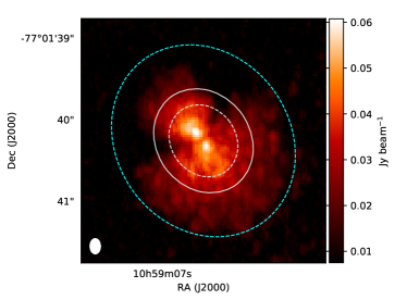
(a) The moment 8 map of ¹²CO line emission

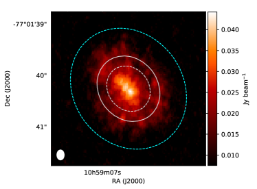
(b) The moment 8 map of ¹³CO line emission

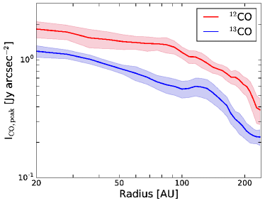
(c) The azimuthally averaged I_ν,peak profile

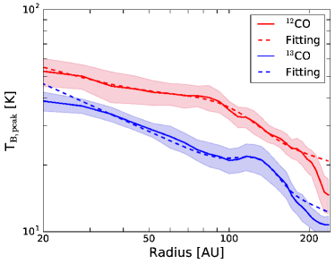
(d) The T_B,peak profile

Figure 4: The moment 8 maps of (a) ¹²CO and (b) ¹³CO line emission with dust continuum. The absorption feature is seen in the northern half-disk. The overlaid white and cyan dashed ellipses are the same as those in Figure 1. The white solid contour indicates the location of the bump at 130 au in the azimuthally averaged ¹³CO peak intensity radial profile. (c) The azimuthally averaged radial profiles of the peak intensity (I_ν,peak) of ¹²CO (red) and ¹³CO (blue) lines in the southern half-disk which is not affected by the absorption features. The color-shaded regions indicate the uncertainties due to the azimuthal average. There is a small bump in I${}_{\rm{}^{13}CO,peak}$ around 130 au.(d) The radial profiles of the peak brightness temperature (T_B,peak) derived from the I_ν,peak of ¹²CO (red) and ¹³CO (blue) lines. The color-shaded regions indicate the uncertainties propagated from those of I_ν,peak. The dashed lines present the lease square fitting results with Equation 2. The derived T_B,peak from the I${}_{\rm{}^{13}CO,peak}$ profile also shows a small bump at $\rm r\sim 130$ au.

Table 3: The fitting parameters of the peak brightness temperature profiles of the ¹²CO and ¹³CO lines.

Species	$A$	$B$	$C$	$D$	$E$
	[K]		[K]	[au]	[au]
12CO	37.57$\pm$1.38	$-$0.38$\pm$0.02	8.37$\pm$0.91	82.81$\pm$4.65	36.05$\pm$5.69
13CO	28.29$\pm$0.38	$-$0.54$\pm$0.03	4.31$\pm$0.69	127.62$\pm$3.33	21.96$\pm$4.86

3.2 The azimuthally averaged intensity profiles

To investigate the radial structure of dust and gas disks, we make the azimuthally averaged radial profiles of the images in Figure 1. The derived disk inclination of $31^{\circ}$ and disk PA of $36.2^{\circ}$ are applied to calculate the projected disk radius of each pixel. We azimuthally average every 8 au width annulus inside $\rm r\lesssim 240$ au. As mentioned in Section 3.1, the CO isotopologue lines are affected by the absorption feature in the northern half-disk against the disk minor axis. We azimuthally average only the southern half-disk (PA = 126.2^∘ to 306.2^∘, counterclockwise from the North) for the CO isotopologue lines to avoid the absorption feature. Meanwhile, since the dust continuum is free to line absorption feature, we average the full azimuthal angles for the dust continuum image.

Figure 3(a) presents the azimuthally averaged radial profile of dust continuum (black) in the $\rm Jy~{}arcsec^{-2}$ unit. The figure also shows the azimuthally averaged integrated intensity radial profiles of ¹²CO (red), ¹³CO (green), and C¹⁸O (blue) line in the $\rm Jy~{}arcsec^{-2}~{}km~{}s^{-1}$ unit. We integrate the intensities of the CO isotopologue lines within the same velocity range from $\rm\sim-1~{}km~{}s^{-1}$ to $\rm\sim 12~{}km~{}s^{-1}$. The color-shaded regions indicate the uncertainties of the (integrated) intensity profiles due to the azimuthal average. As shown in Figure 1(a), there is a dust gap at $\rm r\sim 90$ au and a dust ring at $\rm r\sim 120$ au. Compared with the rapid drop of the dust continuum intensity around 90 au, the CO isotopologue emission lines are extended to $\rm r\sim 240$ au.

Figure 3(b) presents the ratios between the azimuthally averaged integrated intensities of the CO isotopologue lines: ¹³CO/¹²CO (green), C¹⁸O/¹²CO (red), and C¹⁸O/¹³CO (blue). The color-shaded regions indicate the uncertainties of the line ratios due to those of azimuthally averaged integrated CO intensities in Figure 3(a). We note that even if we derive the line ratios by dividing the moment 0 maps first and then averaging azimuthally, the results are identical inside 200 au. In the region outside of 200 au, the signals are weak so that the line ratios have very large uncertainties.

The line ratios show that the ¹²CO and ¹³CO lines are optically thick toward the CR Cha disk because the measured line ratios between three CO isotopologue emission lines are larger than 0.2 at all radii, which is larger than the typical abundance ratio of ¹³CO:¹²CO = 1:67 and C¹⁸O:¹³CO = 1:7 in protoplanetary disks (e.g., Qi et al., 2011). When the molecular lines are optically thin, the line ratios should be almost the same as the abundance ratios because the line strength is proportional to the column density of the molecules. Meanwhile, when the lines are optically thick, the intensity at the line center becomes the same as the blackbody radiation and irrelevant to the molecular abundances. Thus, the line ratios do not need to be close to the abundance ratios.

3.3 The peak brightness temperatures of the CO isotopologue lines

Since ¹²CO and ¹³CO lines are optically thick, we can adapt the brightness temperature of these lines as a gas temperature. To estimate the CO gas temperature, we make the moment 8 maps of ¹²CO and ¹³CO emission lines using immoments command in CASA. The moment 8 map shows the peak intensity (I_ν,peak) at each pixel in the data cube.  For making the moment 8 maps, we used the data cube of ¹²CO and ¹³CO emission lines without dust continuum subtraction. The line plus continuum intensity should be used in order to derive the gas temperature from the peak brightness temperature of an optically thick line (e.g., Weaver et al., 2018).

Figure 4(a) and (b) present the moment 8 maps of ¹²CO and ¹³CO line emissions including the dust continuum. The white and cyan ellipses are the same as those in Figure 1. The white solid contour indicates the location of the bump at 130 au in the peak intensity and the peak brightness temperature of ¹³CO line emission in Figure 4(c) and (d). We azimuthally average only the southern half-disk of the moment 8 maps to derive the I_ν,peak radial profiles for avoiding the absorption feature. Figure 4(c) shows the derived I_ν,peak radial profiles of ¹²CO (red) and ¹³CO (blue). The color-shaded regions present the uncertainties due to the azimuthal average. The $\rm I_{B,peak,^{13}CO}$ profile shows a small bump around $\rm r\sim 130$ au, corresponding to the radius of the dust ring beyond the dust gap.

Using the I_ν,peak profiles, we derive the peak brightness temperature (T_B,peak) by assuming $\rm I_{\nu,peak}=B_{\rm\nu}(T_{\rm B,peak})$ where B_ν is the Planck function at a given frequency $\nu$. The derived T_B,peak profiles are presented in Figure 4(d). The color-shaded regions are the uncertainties of T_B,peak due to those of I_ν,peak in Figure 4(c). As the same as I${}_{\rm{}^{13}CO,peak}$ profile, the derived T_B,peak profile from ¹³CO line also shows a small bump at $\sim 130$ au.

To quantify the temperature bump at $\sim 130$ au, we do the least square fit to the derived T_B,peak profiles using the power-law profile with a single Gaussian,

$${\rm T_{\rm B,peak}}(r)=A\left(\frac{r}{\rm 50~{}au}\right)^{B}+C~{}{\rm exp}\left(-\frac{(r-D)^{2}}{2E^{2}}\right)$$ (2)

where $A$, $B$, $C$, $D$, and $E$ are the fitting parameters. Using the data within $\rm 20~{}au\leq r\leq 200~{}au$, we obtain the fitting parameters, as summarized in Table 3. The fitting parameters show that the small bump of T${}_{\rm B,peak,^{13}CO}$ profile at $\rm r\sim 127$ au has $\sim 4.3$ K amplitude, corresponding to $\sim 1.4\sigma$ at this radius ($1\sigma\approx 3$ K). The dashed lines in Figure 4(d) present the fitting results of T_B,peak profiles.

The T_B,peak profile derived from I${}_{\rm{}^{12}CO,peak}$ also has a small bump at $\rm r\sim 82$ au, the inner edge of the dust gap. It may be related to the slope change of the dust continuum intensity. The location of the photosphere of the ¹²CO line could change inside and outside of the dust rich disk. The disk scale height could also change there (see Section 4.4). The difference between the ¹²CO and ¹³CO brightness temperatures can be a hint for the temperature and density distribution of the gas disk. We will discuss it more in Section 4.4.2.

4 Discussion

4.1 The dust gap in the CR Cha disk

To analyze the dust gap structure of the CR Cha disk, we derive the radial profile of dust surface density ($\Sigma_{\rm dust}$) from the observed dust continuum intensity. We derive the optical depth at 225 GHz, $\tau_{\rm 225GHz}$, using the radiative transfer equation, $\rm I_{\rm cont}=B_{\rm 225GHz}(T_{\rm dust})\left(1-exp(-\tau_{\rm 225GHz})\right)$, where we simply assume that the dust temperature is equal to the gas temperature derived from the moment 8 maps of the ¹²CO or ¹³CO line in Figure 4(d), that is, $\rm T_{\rm dust}=T_{\rm gas}=T_{\rm B,peak}$. We note that since both CO lines are optically thick, we can use the derived T_B,peak profiles as the gas temperature (T_gas) profiles of the ¹²CO and ¹³CO line emitting regions. And then we derive the dust surface density $\Sigma_{\rm dust}$ using the equation $\tau_{\rm 225GHz}=\kappa_{\rm 225GHz}\Sigma_{\rm dust}$ where $\rm\kappa_{\rm 225GHz}=2.3~{}cm^{2}~{}g^{-1}$ (e.g., Beckwith et al., 1990) is the dust opacity at 225 GHz.

The solid lines in Figure 5 present the derived $\tau_{\rm 225GHz}$ and $\Sigma_{\rm dust}$ profiles when the T_dust equals T${}_{\rm B,peak,^{12}CO}$ (red) and T${}_{\rm B,peak,^{13}CO}$ (blue). The color-shaded regions indicate the uncertainties of $\tau_{\rm 225GHz}$ and $\Sigma_{\rm dust}$ propagated from those of the peak brightness temperature in Figure 4(d). We note that although we simply assume $\rm T_{dust}=T_{gas}$, the dust temperature near the disk midplane could be lower than the gas temperature of the ¹³CO or ¹²CO line emitting regions (see Section 4.4.2). Thus, the derived dust surface density could be lower than the actual dust surface density.

We adopt a single Gaussian function to estimate the dust gap structure at $\rm r\sim 90$ au. As the baseline of dust surface density profile, we adopt the power-law function with an exponential tail,

$$\Sigma_{\rm d,baseline}=A\left(\rm\frac{r}{50~{}au}\right)^{-0.5}~{}{\rm exp}\left[\rm-\left(\frac{r}{100~{}au}\right)^{4}\right]$$ (3)

where $A=\rm 0.09~{}g~{}cm^{-2}$ for $\rm T_{\rm dust}=T_{\rm B,peak,^{12}CO}$ and $A=\rm 0.13~{}g~{}cm^{-2}$ for $\rm T_{\rm dust}=T_{\rm B,peak,^{13}CO}$. We note that the terms of Equation (3) is derived by the least square fitting to reproduce the shape of the profiles. And then, we choose concrete numbers within the uncertainties of the fitting parameters. After subtracting the baseline from the derived $\Sigma_{\rm dust}$ profiles, the gap structure is fitted using a single Gaussian function,

$$\rm\Sigma_{\rm d,gap}=\Sigma_{peak}\exp\left[\frac{(r-r_{cent})^{2}}{2(\Delta r)^{2}}\right].$$ (4)

Table 4 summarizes the Gaussian fitting parameters for the gap structure. The uncertainties of the fitting parameters are more than 500% for all parameters due to the small number of data points in the gap: only $2-3$ data points are included in the gap width $\sim 8$ au due to 8 au width of annuli for the azimuthal average under the beam size of $\sim 0.087^{\prime\prime}$ ($\sim 16$ au at $d\sim 187.5$ pc).

The dotted lines in Figure 5 presents the fitting results of the baseline plus dust gap. For both cases, the fitting results show that the dust gap is centered at $\rm r\sim 90$ au and has the width of $\sim 8$ au on average. The depth of the gap is measured as $\left(\Sigma_{\rm d,baseline}(\rm r_{cent})-\Sigma_{\rm peak}\right)/\Sigma_{\rm d,baseline}(\rm r_{cent})$, the ratio between the bottom of the gap and the baseline value at the gap center $\rm r_{cent}$. The derived gap depth is $\sim 20\%$ on average. We note that the derived gap depth should be regarded as the upper limit due to the larger synthesized beam size ($\sim 16$ au) than the estimated gap width $\sim 8$ au. The observed intensity profile can be reproduced by a deeper and narrower gap than those derived from our observation. As an example, the observation of HD 163296 disk with high angular resolution ($\sim 0.05^{\prime\prime}$, Isella et al., 2018) shows that the gap is deeper than that observed with low angular resolution ($\sim 0.2^{\prime\prime}$, Isella et al., 2016).

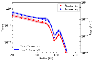
Figure 5: The radial profiles of optical depth at 225 GHz ($\tau_{\rm 225GHz}$) and the dust surface density ($\Sigma_{\rm dust}$), where $\tau_{\rm 225GHz}=\kappa_{\rm 225GHz}\Sigma_{\rm dust}$ with the constant $\kappa_{\rm 225GHz}$=2.3 cm² g^-1. The solid lines present the derived $\tau_{\rm 225GHz}$ and $\Sigma_{\rm dust}$ profiles when we adopt the peak brightness temperature of ¹²CO (red) and ¹³CO (blue) as dust temperature. The color-shaded regions indicate the unceratinties propagated from those of the peak brightness temperature in Figure 4(d). The Gaussian fitting results of the baseline plus dust gap expressed in Equation (3) and (4) are shown as dotted lines with the same color indications. The fitting parameters summarized in Table 4 show that the dust gap is centered at $\rm r\sim 90$ au with a width of $\sim 8$ au on average. The depth of the gap at the center is $\sim 20\%$ on average.

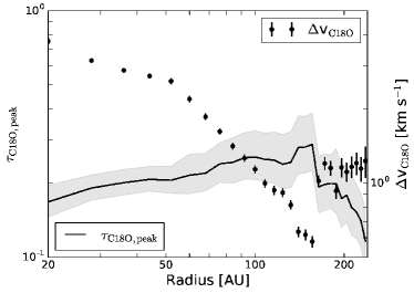
(a) $\tau_{\rm C^{18}O,peak}$ radial profile

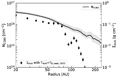
(b) N${}_{\rm C^{18}O}$ radial profile

Figure 6: (a) The radial profile of $\tau_{\rm C^{18}O,peak}$ (solid line) with the uncertainty (gray-shaded regions). The dotted line with error bars indicates the fitted width of the averaged C¹⁸O line spectra at each annulus. The optical depth in the inner disk decreases due to the line broadening caused by the high rotation velocity in the very inner disk. This line broadening leads to small Gaussian peak. (b) The radial profiles of the C¹⁸O column density N${}_{\rm C^{18}O}$ (solid line) with the uncertainty (gray-shaded region). The dotted line with error bars indicates the dust surface density profile derived using $\rm T_{\rm dust}=T_{\rm B,peak,^{13}CO}$ in Section 4.1. The gas disk is extended much further than the dust disk.

Table 4: The Gaussian fitting parameters for the dust gap

Tdust	rcent	$\Delta$r	$\Sigma_{\rm peak}$	Depth
	[au]	[au]	[g cm-2]	[%]
T${}_{\rm B,peak.^{12}CO}$	88.94	9.74	0.028	$\sim 21.71$
T${}_{\rm B,peak.^{13}CO}$	91.47	6.72	0.038	$\sim 19.94$

4.2 C¹⁸O gas column density

In this section, we analyze the CO gas radial distribution in the CR Cha disk. We adopt the following equation in Yamamoto (2017) to derive the C¹⁸O column density (N${}_{\rm C^{18}O}$):

$$\begin{split}\int{\tau_{\nu}\rm dv}&\approx\sqrt{2\pi}~{}\tau_{\rm\nu,peak}\Delta\rm v\\  =&\frac{8\pi^{3}S\mu_{0}^{2}}{3hU(\rm T_{gas})}\left[ \exp\left(\frac{h\nu}{k_{B}\rm T_{gas}}\right)-1\right] \\ &\times\exp\left(-\frac{E_{u}}{k_{B}\rm T_{gas}}\right)N_{\rm molecule}\\ \end{split}$$ (5)

where $\tau_{\rm\nu,peak}$ is the peak optical depth of the molecular line at the line center, $\Delta$v is the width of the molecular line, $S$ is the molecular line strength, $\mu_{0}$ is the permanent dipole moment of the molecule, $h$ is the Planck constant, $U(\rm T_{\rm gas})$ is the rotational partition function of the molecular species at a given gas temperature T_gas, $\nu$ is the rest frequency of the molecular transition line, $k_{\rm B}$ is the Boltzmann constant, $E_{u}$ is the upper state energy level, and $N_{\rm molecule}$ is the column density of the molecule, respectively. We simply assume that the line optical depth has a Gaussian profile with the peak value of $\tau_{\rm\nu,peak}$ and the width of $\rm\Delta v$ for $\rm\int\tau_{\nu}dv\approx\sqrt{2\pi}\tau_{\rm\nu,peak}\Delta v$.

For C¹⁸O $J=2-1$ transition line, we adopt $\rm\nu=219.5603~{}GHz$, $S\mu_{0}^{2}=0.02440~{}{\rm D}^{2}\approx 2.440\times 10^{-51}~{}{\rm J\cdot m^{3}}$, and $E_{u}/k_{B}=15.80580~{}\rm K$ from the Leiden Atomic and Molecular Database (Schöier et al., 2005) and Cologne Database for Molecular Spectroscopy (Müller et al., 2001). The rotational partition function $U(\rm T_{\rm gas})$ of C¹⁸O molecule is approximated as $U(\rm T_{\rm gas})\approx 0.38\left(\rm T_{\rm gas}+0.88\right)$ (Mangum & Shirley, 2017).

As a first step, we derive the peak optical depth at the C¹⁸O line center ($\tau_{\rm C^{18}O,peak}$) using the radiative transfer equation, $\rm I_{\rm C^{18}O,peak}=B_{\rm C^{18}O}(T_{\rm gas})\left[1-\exp(-\tau_{\rm C^{18}O,peak})\right]$ with $\rm T_{gas}=T_{B,peak,^{13}CO}$, the blue line in Figure 4(d). The I${}_{\rm C^{18}O,peak}$ is derived from the Gaussian fitting of the azimuthally averaged C¹⁸O line spectra of every 8 au width annulus within $\rm r\lesssim 240~{}au$.  When we azimuthally average the C¹⁸O line spectra, we shift the velocity offset of the line at each point in the annulus (mainly due to Doppler shift by the Keplerian rotation) by using the moment 1 map of the C¹⁸O line.

From the azimuthally averaged line spectra, we obtain the peak C¹⁸O line intensity (I${}_{\rm C^{18}O,peak}$) and the width ($\Delta$v${}_{\rm C^{18}O}$) by Gaussian fitting.  The peak optical depth of C¹⁸O line ($\tau_{\rm C^{18}O,peak}$) is presented in Figure 6(a) as solid line. The gray-shaded region shows the uncertainty of the $\tau_{\rm C^{18}O,peak}$. The dotted line with error bars in the same figure shows the fitted line width $\Delta$v${}_{\rm C^{18}O}$.  The decrease of $\tau_{\rm C^{18}O}$ in the inner disk is caused by the line broadening. Since the Keplerian rotation velocity is higher and the gradient of velocity along the line of sight is steeper, the beam averaged line width becomes broader in the inner disk. Due to this line broadening, the $\tau_{\rm C^{18}O,peak}$ profile is nearly flat up to $\rm r\sim 160$ au but the line width rapidly decreases. In the outer disk of $\rm r\gtrsim 160~{}au$, the Gaussian fitting is affected by the noise next to the line signal making broader line width and smaller peak intensity. It makes the drop of $\tau_{\rm C^{18}O,peak}$ at $\rm r>160~{}au$.

Finally, we derive the C¹⁸O column density (N${}_{\rm C^{18}O}$) by assigning the derived $\tau_{\rm C^{18}O,peak}$, $\rm\Delta v_{C^{18}O}$, and $\rm T_{gas}=T_{B,peak,^{13}CO}$ into Equation (5). Figure 6(b) shows the derived N${}_{\rm C^{18}O}$ profile as a solid line and their uncertainty as a gray-shaded region. Compared with the derived dust surface density profile, the dotted line with error bars, the C¹⁸O gas disk is much extended than the dust disk. There is no gas gap around the dust gap at $\rm r\sim 90$ au due to the large synthesized beam size of the line observation.

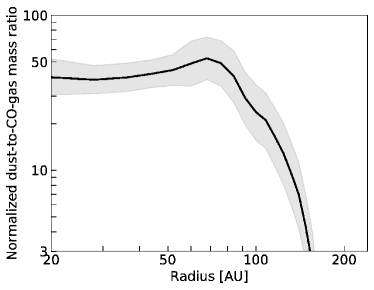
(a) The normalized dust-to-CO-gas mass ratio

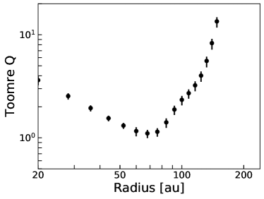
(b) Toomre Q parameter

Figure 7: (a) The radial profile of dust-to-CO-gas mass ratio ($\epsilon/X$) normalized by the typical ratio in the interstellar medium ($\epsilon_{0}/X_{0}$). The $\Sigma_{\rm dust}$ profile is convolved with the same beam size of C¹⁸O line image for deriving the dust-to-CO-gas mass ratio. The gray-shaded region indicates the uncertainty of the ratio. The disk region in $\rm r\lesssim 80~{}au$ has $\sim 50$ times higher dust-to-CO-gas mass ratio than the typical interstellar medium. Outside of the dust ring at 120 au, the ratio rapidly decreases toward the unity. (b) The Toomre’s Q parameter of the disk derived from the $\Sigma_{\rm dust}$ in Figure 6(b) and the assumption of $\Sigma_{\rm disk}\approx\Sigma_{\rm gas}=100\Sigma_{\rm dust}$. The region $\rm r\lesssim 80~{}au$ has $\rm Q\approx 1-3$, which is marginally gravitationally unstable disk.

4.3 The dust-to-CO-gas mass ratio

The dust-to-gas mass ratio is one of the important parameters to understand the physical and chemical conditions of the protoplanetary disks. Based on the radial profiles of dust surface density and C¹⁸O column density in Section 4.1 and 4.2, we derive the dust-to-CO-gas mass ratio of the CR Cha disk.

When we adopt the factor $X\equiv\rm N_{CO}/N_{H_{2}}$, the ratio of the number density between CO and H₂ molecules, and $\epsilon\equiv\Sigma_{\rm dust}/\Sigma_{\rm H_{2}}$, the dust to gas mass ratio, we derive the dust-to-CO-gas mass ratio

$$\frac{\epsilon}{X}=\frac{\Sigma_{\rm dust}}{\Sigma_{\rm H_{2}}}\frac{\rm N_{\rm H_{2}}}{\rm N_{\rm CO}} =\frac{\Sigma_{\rm dust}}{\rm 2m_{H}N_{CO}}=14~{}\frac{\Sigma_{\rm dust}}{\Sigma_{\rm CO}}$$ (6)

where $\rm\Sigma_{H_{2}}=2m_{H}N_{H_{2}}$, $\rm\Sigma_{CO}=28m_{H}N_{CO}$, and $\rm m_{\rm H}=1.67\times 10^{-24}~{}g$ is the mass of hydrogen atom. If we adopt the typical abundance ratio of $\rm{}^{12}CO/C^{18}O$ $=444$ (e.g., Qi et al., 2011), the CO number density is derived by the conversion of $\rm N_{CO}=444~{}N_{C^{18}O}$. We adopt the typical values in the ISM of $X_{0}=10^{-4}$ and $\epsilon_{0}=10^{-2}$ for the comparison to the typical dust-to-CO-gas mass ratio in the interstellar medium (ISM).

Figure 7(a) presents the radial profile of the normalized dust-to-CO-gas mass ratio $\left(\epsilon/X\right)/\left(\epsilon_{0}/X_{0}\right)$, indicating how the dust-to-CO-gas mass ratio of the CR Cha disk deviates from the typical ISM value. The gray-shaded region indicates the uncertainty of the dust-to-CO-gas mass ratio based on the uncertainties of the derived $\Sigma_{\rm dust}$ and N${}_{\rm C^{18}O}$. We note that the $\Sigma_{\rm dust}$ profile is convolved with the same beam size of C¹⁸O line image for deriving the dust-to-CO-gas mass ratio. In the disk radius of $\rm r\lesssim 80~{}au$, the dust-to-CO-gas mass ratio is $\sim 50$ times higher than the typical ISM value.

The dust concentration by the radial drift of dust grains is one of the possible mechanisms to explain this high dust-to-CO-gas mass ratio in the inner disk. Here, we simply assume that the initial dust disk is extended to $\rm r=240$ au with a uniform dust surface density and the dust mass is conserved during the radial contraction. If only dust grains drift inward down to $\rm r\sim 90$ au from $\rm r=240$ au, $\sim 9$ times dust concentration is acceptable. However, it is still not enough to reach $\sim 50$ times higher dust-to-CO-gas mass ratio so that they may need other causes to increase the dust-to-CO-gas mass ratio. The CO gas depletion ($X=\rm N_{CO}/N_{H_{2}}<10^{-4}$) and/or gas dispersal ($\epsilon=\rm\Sigma_{dust}/\Sigma_{gas}>0.01$) may have to be considered as another possibility to explain this high dust-to-CO-gas mass ratio.

We note that there are some uncertainties in the derived dust-to-CO-gas mass ratio. As mentioned in Section 4.2, the dust surface density could be underestimated because the temperature at the disk midplane, where optically thin dust continuum will be mainly emitted, is possibly lower than the temperature of the ¹³CO line emitting region in the disk surface. In that case, the dust-to-CO-gas mass ratio could be underestimated. Also, the dust opacity has large uncertainty, which, too, leads to uncertainty in derived dust surface density. Meanwhile, if the C¹⁸O line is optically thick, the derived C¹⁸O column density will be underestimated. Thus, the derived dust-to-CO-gas mass ratio could be overestimated.

Although we can reproduce the observed high dust-to-CO-gas ratio with dust concentration, gas dispersal, or CO depletion, this high dust-to-CO-gas mass ratio can trigger the gravitational or streaming instabilities. The disk stability by self-gravity is presented by the Toomre Q parameter (Toomre, 1964),

$$Q\equiv\frac{c_{\rm s}\Omega_{\rm K}}{\pi G\Sigma_{\rm disk}},$$ (7)

where $c_{\rm s}$ sound speed, $\Omega_{\rm K}$ orbital frequency, G gravitational constant, and $\Sigma_{\rm disk}$ disk surface density. The assumption of $\rm T=T_{\rm B,peak,^{13}CO}$ and $M_{\star}=1.657~{}M_{\odot}$ are used for deriving $c_{\rm s}=\sqrt{\rm kT/\mu m_{\rm H}}$ and $\Omega_{\rm K}=\sqrt{GM_{\star}/r^{3}}$. If the observed high dust-to-CO-gas mass ratio is explained only by the CO gas depletion and there is no gas dispersal or dust concentration ($\rm\Sigma_{disk}\approx\Sigma_{gas}=100\Sigma_{dust}$), the derived Toomre Q parameter is $\rm Q\sim 1-3$ inside of $\rm r\sim 100$ au, shown in Figure 7(b), indicating that the disk is marginally unstable by self-gravity. Meanwhile, if there is gas dispersal and/or dust concentration, Figure 9 in Yang et al. (2017) shows that $\Sigma_{\rm dust}/\Sigma_{\rm gas}\gtrsim 0.2$ triggers the streaming instability regardless of the grain sizes. It indicates that $(\epsilon/X)/(\epsilon_{0}/X_{0})\gtrsim 20$ can trigger the streaming instability if we assume no CO gas depletion (that is, $X=N_{\rm CO}/N_{\rm H_{2}}=10^{-4}$). If these instabilities are triggered, the dust disk is rapidly dissipated by creating planetesimals or disk substructures like spiral arms and cannot stand for a long time (e.g., Dong et al., 2015a; Li et al., 2019). Since it is not consistent with the observation, some assumptions used in the derivations of dust and gas surface density from our observations may not be realistic.

4.4 The formation of dust gap-ring structure

In this section, we discuss the possible formation mechanisms of the dust gap-ring structure in the outer region of the dust disk. Here, we introduce two possible mechanisms: gap opening by a planet and dust concentration on the gas pressure bump at the outer edge of the dust disk.

4.4.1 Gap opening by a planet

The surface density distribution of the gap formed by a planet is well studied by numerical simulations in previous studies. Here, we compare the surface density distribution around the gap obtained from the observations with the numerical models to constrain the planet mass which can reproduce the observed gap structure.

We adopt the model of Rosotti et al. (2016) to estimate the minimum planet mass for reproducing the dust gap structure in the CR Cha disk. They suggest that the minimum planet mass can perturb the dust surface density is

$$M_{\rm p,min}\sim 15~{}M_{\oplus}\left(\frac{H/R}{0.05}\right)^{3}\left(\frac{M_{\ast}}{1~{}M_{\odot}}\right)$$ (8)

where $H$ is the disk vertical scale height, $R$ is the radial location of the planet, and $M_{\ast}$ is the central star mass. To evaluate $H/R$, we use $\rm T=22$ K at the gap center of $\rm r_{cent}=R=91.47$ au, which are obtained from ¹³CO line emission and from the dust surface density distribution. Assigning $M_{\ast}=1.657~{}M_{\odot}$ Villebrun et al. (2019) and $H/R=0.0683$ into Equation (8), we obtain $M_{\rm p,min}\sim 0.2~{}M_{\rm J}$. This is the lower limit of the planet mass for creating a dust gap in the CR Cha disk.

Next, we evaluate the planet mass in the gap through the fitting of the observed gap structure using Equation (6)-(10) in Kanagawa et al. (2017). In Kanagawa et al. (2017), the surface density profile is controlled by two parameters, $K$ and $K^{\prime}$:

$$K=\left(\frac{M_{\rm p}}{M_{\ast}}\right)^{2}\left(\frac{h_{\rm p}}{R_{\rm p}}\right)^{-5}\alpha^{-1},$$ (9)

$$K^{\prime}=K\left(\frac{h_{\rm p}}{R_{\rm p}}\right)^{2},$$ (10)

where $M_{\rm p}$ is the planet mass, $M_{\ast}$ is the central star mass, $h_{\rm p}$ is the disk scale height at the planet orbital radius $R_{\rm p}$, and $\alpha$ is the dimensionless parameter for the strength of the turbulence Shakura & Sunyaev (1973). To evaluate these parameters, we use the same parameters used above: $\rm T=22~{}K,~{}r_{cent}=91.47~{}au$. The gap center is also used as the planet orbital radius $R_{\rm p}$. Using these values, we find that the parameters $K$ and $K^{\prime}$ depend on a single parameter $\alpha^{-1}(M_{\rm p}/M_{\ast})^{2}$.

Figure 8 shows the comparison between the surface density distributions derived from the observation (filled square) and predicted by the model of gap opening by a planet (solid line). We note that we normalize the observed dust surface density by the baseline function Equation (3) for the fitting to the model.  The best fit value is $\alpha^{-1}(M_{\rm p}/M_{\ast})^{2}=3.3\times 10^{-5}$. Thus, the planet mass can open the observed gap structure is

$$M_{\rm p}=0.99M_{\rm J}\left(\frac{\alpha}{0.01}\right)^{0.5},$$ (11)

where $M_{\rm J}$ is the Jupiter mass. Note that the planet mass estimated here has a large uncertainty caused by the resolution of the observations and the dust evacuation from the gap as mentioned above.

We note that there are two uncertainties for this planet mass estimation. First, the observed gap structure is not well resolved by the beam as mentioned in Section 4.1. Thus, the gap in the dust surface density would be deeper than that obtained from the observations. Second, the depth of dust gap may be much deeper than that of the gas gap. We assume that the dust gap structure obtained from our observation can trace the gas gap structure. This assumption will be justified when the dust grain size is small enough so that the dust grains are tightly coupled with the gas.  In contrast, dust particles will be evacuated from the gas gap if the dust particles grow to about mm size de Juan Ovelar et al. (2013); Dong et al. (2015b). In this case, we obtain the depth of the gas gap larger than the real, which concludes a more massive planet mass to reproduce the observed gap depth.

We also estimate the upper limit of the planet mass from the cases that the gas gap is too shallow or too wide to be non-detection within the uncertainties of our observation. The ratio of the derived lower and upper limit of N${}_{\rm C^{18}O}$ at 100 au is $\sim 0.6$. If we assume that the upper limit is the baseline value and the lower limit is the bottom of the gas gap,

$$\frac{\Sigma_{\rm lower}}{\Sigma_{\rm upper}}=\frac{1}{1+0.04K}>0.6.$$ (12)

When we assign the $R_{\rm p}=91.47$ au, $\rm T=22$ K, and $M_{\ast}=1.657~{}\rm M_{\odot}$ into Equation (12), the estimated upper limit of the planet mass is

$$M_{\rm p}<0.87M_{\rm J}\left(\frac{\alpha}{0.01}\right)^{1/2}.$$ (13)

Similarly, if the gas gap has a comparable width with the synthesized beam size of our observation, we also cannot detect the gas gap in the N${}_{\rm C^{18}O}$ profiles. The relation between the gap width and the planet mass is expressed as

$$\Delta R=0.33K^{\prime 1/4}R_{\rm p}.$$ (14)

Considering the beam size of $\sim 0.2"$ corresponding to $\sim 37.6$ au at 187.5 pc in physical scale, the upper limit of the planet mass is derived as

$$M_{\rm p}<1.2M_{\rm J}\left(\frac{\alpha}{0.01}\right)^{1/2}.$$ (15)

Those values conclude that about Jupiter-mass planets are required to reproduce the observed dust gap structures regardless of the existence of the gas gap at the dust gap location. The scattered light imaging is a good next step to investigate the planet mass estimation and gap structures by their higher spatial resolutions and direct tracing of small dust grains that are generally well-couple with the gas (e.g., Dong & Fung, 2017).

The temperature bump around 130 au could be related to the heating of the outer wall of the gap. According to the previous studies, the gap opening by a planet changes the temperature distribution around the gap structure (e.g., Jang-Condell & Turner, 2012; Turner et al., 2012). Due to the smaller surface density inside the gap structure, this region can be heated by the stellar radiation which can penetrate to a deeper layer of the disk.

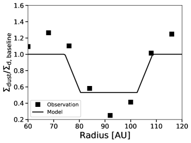
Figure 8: Comparison between the surface density profiles derived from our observation (filled squares) and predicted by the gap opening model (solid line). The vertical axis is the surface density normalized by the baseline function expressed as Equation 3.

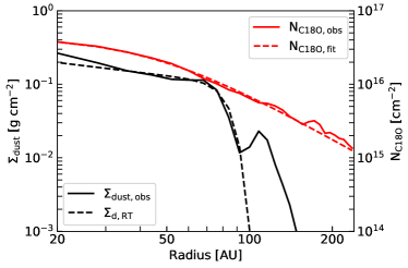
(a) The $\Sigma_{\rm dust}$ and N${}_{\rm C^{18}O}$ profiles

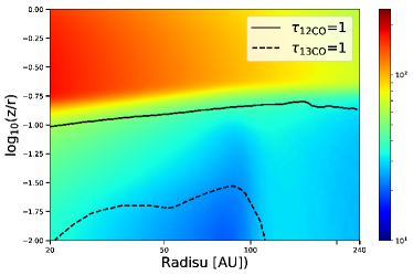
(b) The T_gas distribution in the disk r-z plane

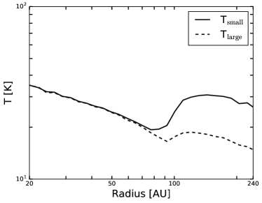
(c) The T_dust distribution at the disk midplane

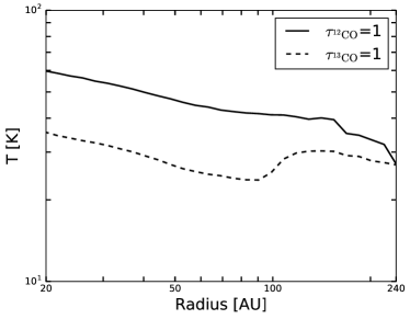
(d) The T_gas distribution at the photosphere of the ¹²CO and ¹³CO lines

Figure 9: (a) The dust surface density profile (black) and C¹⁸O column density (red) profile derived from our observations (solid) and the fitting results (dashed) of Equation (16) and (19). (b) The gas temperature distribution in the disk $r-z$ plane derived by the radiative transfer calculation. The solid and dashed lines indicate the photospheres ($\tau_{\nu}=1$) of ¹²CO and ¹³CO emission lines, respectively. (c) The temperature distribution of the small (solid) and large (dashed) dust grains at the disk midplane. The T_small distribution shows a bump beyond the dust gap at 90 au. (d) The gas temperature distribution at the photosphere of ¹²CO (solid) and ¹³CO (dashed) emission lines shown in Figure 9(b). The gas temperature bump around 130 au is seen at the photosphere of ¹³CO line, but no bump at the photosphere of ¹²CO line.

4.4.2 Dust concentration on the gas pressure bump

Here, we discuss another possible formation mechanism of the dust gap-ring structure in the outer region of the dust disk. We assume the situation that the dust disk becomes more compact than the gas disk through the radial drift of the dust grains in the disk. At the outer edge of the dust disk, the transition of optical depth occurs due to the steep decrease of dust surface density. Then, the temperature at the midplane increases by the direct irradiation heating from the hot surface layer of the disk. This temperature variation leads to the pressure bump formation just beyond the edge of the dust disk. If there is a small amount of dust grains in the outside of the dust disk, they drift inward and concentrate on the pressure bump so that the ring structure is formed. This mechanism is consistent with the observed features: a dust ring beyond the dust gap, more compact dust disk than the gas disk, and the temperature bump in ¹³CO line emission beyond the dust gap.

We perform the radiative transfer calculation to derive the temperature distributions in the disk $r-z$ plane when the dust disk is more compact than the gas disk by using a published code HO-CHUNK Whitney et al. (2003a, b, 2004, 2013). We adopt the stellar mass of $\rm 1.657~{}M_{\odot}$, the effective temperature of 4800 K, and the stellar radius of $\rm 3.113~{}R_{\rm\odot}$ Villebrun et al. (2019). We also use the dust surface density derived from the observed I_cont at $\rm T_{dust}=T_{B,peak,^{13}CO}$. For the radiative transfer calculations, we use the fitted dust surface density profile within the radius of $\rm 20~{}au<r<100~{}au$ to consider the compact dust disk. Although the dust temperature will change step by step during the radial drift of the grains in reality, here we assume a fixed dust surface density profile for the simplicity. We obtain the fitted dust surface density profile of

$$\Sigma_{\rm d,RT}=A\left(\frac{r}{10\ {\rm au}}\right)^{B}\exp\left[-\left(\frac{r}{C\ {\rm au}}\right)^{10}\right]$$ (16)

where $A=0.27\pm 0.02~{}\rm g~{}cm^{-2}$, $B=-0.45\pm 0.06$, and $C=86.0\pm 1.66$ au. It is presented as the black dashed line in Figure 9(a). The dust distribution is effectively cut off at 100 au.

In our calculation, we introduce two dust components: small dust grains and large dust grains. The minimum and maximum sizes are 0.0025 ${\rm\mu}$m and 0.2 ${\rm\mu}$m for small dust grains and 0.01 ${\rm\mu}$m and 1 mm for large dust grains, respectively. The size distribution of both dust components is $n(a)\propto a^{-3.5}$, where $n(a)$ is the number density per unit radius and $a$ is the radius of dust grains. The opacity models for both small and large dust grains are described in Hashimoto et al. (2015) (see also Kim et al., 1994; Wood et al., 2002; Dong et al., 2012). We adopt Equation (16) as the surface density distribution of large dust grains and assume that the surface density of the small dust grains is 10 times smaller than that of the large dust ($\Sigma_{\rm small}=0.1\Sigma_{\rm large}$; e.g., D’Alessio et al., 2006). We note that the small-to-large dust mass ratio for the size distribution of $n(a)\propto a^{-3.5}$ is 1%. However, many practical calculations (e.g., Andrews et al., 2011; Dong et al., 2015b) use the size distribution and change the small-to-large dust mass ratio independently because the results are not very different even if the mass ratio is assumed as 10%. To obtain the density distributions of small and large dust grains, we set the scale height of them,

$$H_{\rm l}=\rm 2~{}au\left(\frac{r}{100~{}au}\right)^{1.25},$$ (17)

$$H_{\rm s}=\rm 6.5~{}au\left(\frac{r}{100~{}au}\right)^{1.25},$$ (18)

where $H_{\rm l}$ and $H_{\rm s}$ are the scale height of large and small dust grains, respectively. We assume that the scale height of small dust grains is similar to the gas scale height. The scale height of the large dust grains is assumed to be about three times smaller than that of the small dust grains . Using these scale heights, we evaluate the density of small and large dust grains, whose density distributions in $z$ direction are proportional to $\exp(-z^{2}/(2H_{\rm l,s}^{2}))$. We note that the dependence of model parameters on the resulting disk structures is out of the scope of this work and remains to be explored.

Figure 9(b) shows the temperature distribution in the disk $r-z$ plane generated by the radiative transfer calculation. We overlay the $\tau_{\nu}=1$ layer (i.e., photosphere) of ¹²CO and ¹³CO line emissions as the solid and dashed lines. To obtain the optical depth of the CO isotopologue lines, we evaluate the surface density of ¹²CO and ¹³CO from the C¹⁸O column density obtained from the C¹⁸O line observations, shown as the red solid line in Figure 9(a). We fit the column density as follows,

$$N_{\rm C^{18}O}=A\left[1+\left(\frac{r}{B\ {\rm au}}\right)^{C}\right]^{-1},$$ (19)

where $A=(4.46\pm 0.04)\times 10^{16}~{}{\rm cm^{-2}}$, $B=44.40\pm 0.5$ au, and $C=2.12\pm 0.03$. It is presented as the red dashed line in Figure 9(a). We also assume the abundance ratio of $\rm{}^{12}CO/C^{18}O=444$ and $\rm{}^{12}CO/^{13}CO=67$ (Qi et al., 2011). Since ¹²CO line emission is optically thick, the photosphere of ¹²CO line is seen at the hot upper surface of the disk. On the other hand, since ¹³CO line is marginally optically thick, the photosphere of ¹³CO line is located around or below the disk midplane.

Figure 9(c) shows the temperature distribution of dust grains at the disk midplane obtained from the radiative transfer calculations. The solid and dashed lines indicate the temperatures of small and large dust grains, respectively. The figure shows that T_small starts to increases at the outer edge of the dust gap at $\rm r\sim 90~{}au$. In contrast, T_large does not increase much in the same region of the disk.

The temperature distribution can be explained as follows. The temperature at the disk midplane is determined by the balance between the heating from the hot surface layer irradiated by the stellar radiation and cooling by the dust thermal emission. In the region $\rm r\lesssim 90$ au, the disk is optically thick against the irradiation from the hot surface layer so that the temperature of the large and small dust grains have the same temperature. On the other hand, since the disk is optically thin in the region $\rm r\gtrsim 90$ au, the small and large dust grains are directly irradiated by the hot disk surface. Since the wavelength dependence on the opacity of small dust grains is steeper than that of the large dust grains, the opacity of the small dust grains is higher for the irradiation from the hot disk surface ($\sim 30~{}\mu$m) but lower for their thermal emission ($\sim 100~{}\mu$m) than those of the large dust grains. Thus, the temperature of the small dust grains is higher than that of the large dust grains, resulting in the occurrence of the temperature bump in the region $\rm r\gtrsim 90$ au. Since the gas temperature will be determined by the collisional heating with small dust grains, this temperature distribution causes the gas pressure bump around $\rm r\sim 130$ au. If there is some amount of the dust in the region $\rm r\gtrsim 90$ au, they can be concentrated at this gas pressure bump and form the observed ring structure. Here, we assume that there is enough dust in the region $\rm r>90$ au in addition to Equation (16) to make the ring structure as a result of the radial drift of the dust and to determine the gas temperature with the small dust temperature. We need further investigation of this scenario to justify this assumption.

Figure 9(d) shows the temperature distributions at the photosphere for ¹²CO line emission as solid line. There is no temperature bump beyond the dust gap at 90 au since it is at the hot upper disk surface. We also show the temperature distribution at the photosphere of the ¹³CO line emission as a dashed line, but we plot the midplane temperature if the photosphere of ¹³CO line is located below the midplane. Since the optical depth of ¹³CO line emission is smaller than that of ¹²CO line, it traces the temperature at the layer closer to the midplane so that there is a bump in temperature distribution in the region $\rm r\gtrsim 90$ au. This is consistent with the observed intensity bump of ¹³CO line around 130 au but nothing for the ¹²CO line. On the other hand, the C¹⁸O line is optically thin and intensities in 20 K and 30 K are similar in LTE condition. Thus, we cannot see the bump in the C¹⁸O line, too. We note that the optical depth of ¹³CO seems lower than the unity in the region of $\rm r>120$ au because Figure 9(c) shows only the upper half-disk in the z-direction. When integrating the full vertical disk, the optical depth of ¹³CO becomes larger than unity up to $\rm r\sim 160$ au but $\sim 0.7$ in the region $\rm r>160$ au. Considering the large uncertainty of the line ratio in Figure 3(b), it does not significantly conflict with our observations.

Meanwhile, the dust gap-ring structure in the CR Cha disk may be formed through different mechanisms. As shown in Figure 9(c), the dust temperature at the disk midplane inside the dust gap is $\sim 20$ K. Since this is comparable to the CO sublimation temperature ($\sim 15-25$ K), the dust gap and ring could be created by dust sintering effect (Okuzumi et al., 2016). Secular gravitational instability (secular GI Ward, 2000; Youdin, 2011; Michikoshi et al., 2012) is another possible mechanism of dust ring structure formation (Takahashi & Inutsuka, 2014). As mentioned in Section 4.3, the disk has small Q value and/or large dust-to-gas mass ratio. These features are suitable for the growth of the secular gravitational instability in the disk (Takahashi & Inutsuka, 2014, 2016; Latter & Rosca, 2017; Tominaga et al., 2019). Also, the existence of the dead zone is another possible cause to produce the dust gap-ring structure in the disk. If the gas gap is generated at the outer edge of the dead zone by viscous instability (e.g., Flock et al., 2015; Hasegawa & Takeuchi, 2015), dust grains can be piled up there. The temperature bump at the outer edge of the gap is also generated by the heating of dust grains (e.g., Hasegawa & Pudritz, 2010). To distinguish the dust gap-ring formation mechanisms, further investigations are required, for example, the size distribution of the dust particles, since the dust sintering mechanism indicates that the dust radius is small in a dust ring structure.

5 Summary

In this paper, we present the images of the dust continuum at 225 GHz and the CO isotopologue $J=2-1$ emission lines of the CR Cha disk observed by the ALMA. The observed dust continuum image shows a dust gap at $\rm r\sim 90$ au and a faint dust ring at $\rm r\sim 120$ au. We derive the radial profile of dust surface density to investigate the gap-ring structure by assuming the peak brightness temperature of ¹³CO emission line as dust temperature T_dust. Using the Gaussian fitting, we find that the dust gap is located at the radius of 90 au and has the gap depth of $\sim 20\%$ at the gap center with $\sim 8$ au width on average.

We analyze ¹²CO, ¹³CO and C¹⁸O $J=2-1$ emission lines to investigate the gas disk of CR Cha. The moment 8 maps, the channel maps, and the averaged spectra of the CO isotopologue lines inside the radius of 240 au show the absorption feature which might be caused by the Cha I foreground cloud at the velocity of $\sim 4.5$ km s^-1. The azimuthally averaged radial profiles of the integrated CO isotopologue line intensities show that the gas disk is extended up to 240 au, which is much larger than the dust disk. The ratios between the CO isotopologue line emissions are larger than 0.2 at all radii, larger than the typical abundance ratios of CO isotopologue in the protoplanetary disks. It indicates that ¹²CO and ¹³CO lines are optically thick. To derive the gas temperature, we make the moment 8 maps of ¹²CO and ¹³CO lines without dust continuum subtraction because they are optically thick lines. The azimuthally averaged radial profile of the ¹³CO peak intensity shows a small bump around $\sim$130 au, which may indicate the temperature bump in the ¹³CO line emitting region.

We investigate two possible mechanisms to reproduce the observed dust gap at 90 au, the dust ring structure at 120 au, and a bump of ¹³CO emission line at 130 au: gap opening by a planet and dust concentration on the gas pressure bump at the outer edge of the dust gap.

For investigating the scenario of gap opening by a planet, we compare the observed surface density distribution around the gap to the model surface density obtained by numerical simulations done by Kanagawa et al. (2017). We obtain the planet mass of $M_{\rm p}\approx 0.99M_{\rm J}\left(\alpha/0.01\right)^{1/2}$, where $\alpha$ is the turbulent viscous parameter, can reproduce the observed dust surface density around the gap. However, this value has large uncertainties due to some reasons: the synthesized beam size comparable to the gap width only constrains the upper limit of the gap depth and the dust gap structure may not trace the gas gap structure. Thus, this value should be considered as a very rough estimation.

For investigating the scenario of dust concentration on the gas pressure bump at the outer edge of the dust gap, we set the radiative transfer calculation with two dust components: small and large dust grains. When the dust disk becomes more compact than the gas disk by the radial drift of the dust grains in the disk, the steep gradient of dust surface density around the outer edge of the dust disk leads to the efficient heating by the irradiation from the hot upper disk surface to the small dust grains than the large dust grains. As a result, the gas temperature bump beyond the dust disk is produced because the small dust grains are coupled with the gas. It can make the pressure bump and the dust grains may be concentrated at the pressure peak formed beyond the dust disk. Also, since the optical depth of ¹³CO line emission is smaller than that of ¹²CO, it traces the temperature around the midplane so that a bump of ¹³CO line is seen at 130 au, but not for ¹²CO line. We note that the dust sintering, secular gravitational instability, and the existence of the dead zone at the disk midplane also can explain the observed dust gap-ring structure and gas temperature bump beyond the dust gap qualitatively. We need further investigation to develop quantitative interpretation in the future.

Appendix A The channel maps of CO isotopologue lines

We present the channel maps of ¹²CO, ¹³CO and C¹⁸O isotopologue lines to clearly show where the absorption feature is. The black contours overlaid in each panel indicate the Keplerian rotation model with the stellar mass 2 M_⊙, the disk inclination $31^{\circ}$, and disk position angle $36.2^{\circ}$. We used the python code written by Kevin Flaherty for generating the Keplerian rotation model. At the velocity of $\rm V\sim 4.5~{}km~{}s^{-1}$, absorption features appear. The Keplerian mask shows what regions are affected by this absorption in the moment 0 and 8 maps of the CO isotopologue lines (see Figure 1 and 4).

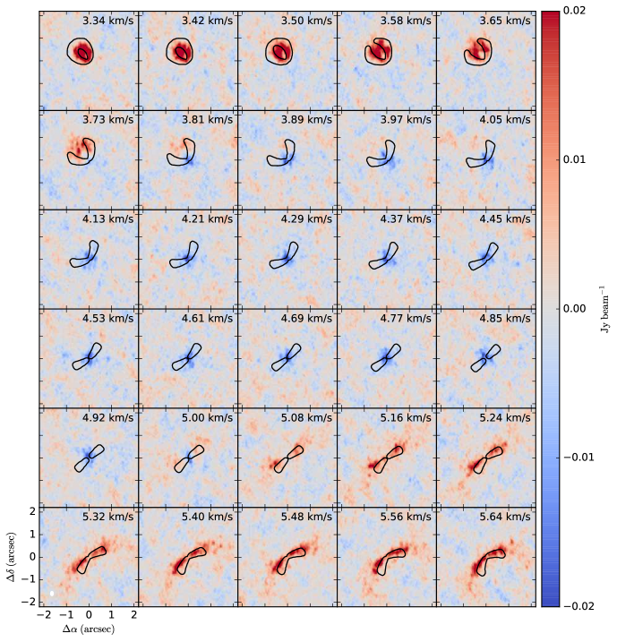
Figure A.1: The ¹²CO $J=2-1$ line channel maps from 3.3 km s^-1 to 5.6 km s^-1. The channels are showing the absorption feature in the velocity of $\rm 3.8<v<5.1~{}km~{}s^{-1}$. The black contours indicate the Keplerian rotation model derived by the 31^∘ disk inclination and 36.2^∘ disk position angle.

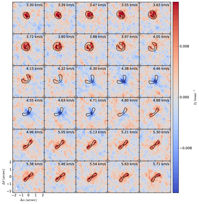
Figure A.2: The ¹³CO $J=2-1$ channel maps from 3.3 km s^-1 to 5.7 km s^-1. The channels are showing the absorption feature in the velocity of $\rm 4.3<v<4.8~{}km~{}s^{-1}$. The black contours indicate the Keplerian rotation model derived by the 31^∘ disk inclination and 36.2^∘ disk position angle.

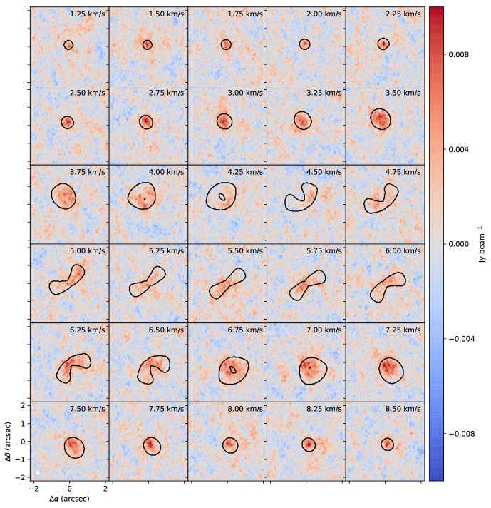
Figure A.3: The C¹⁸O $J=2-1$ channel maps from 1.25 km s^-1 to 8.5 km s^-1 by smoothing the velocity resolution from 0.08 km s^-1 to 0.25 km s^-1 for increasing the signals. There is no clear absorption feature in the velocity of $\rm 4<v<5~{}km~{}s^{-1}$. The black contours indicate the Keplerian rotation model derived by the 31^∘ disk inclination and 36.2^∘ disk position angle.

References

- Andrews et al. (2011) Andrews, S. M., Wilner, D. J., Espaillat, C., et al. 2011, ApJ, 732, 42
- Beckwith & Sargent (1991) Beckwith, S. V. W., & Sargent, A. I. 1991, ApJ, 381, 250
- Beckwith et al. (1990) Beckwith, S. V. W., Sargent, A. I., Chini, R. S., & Guesten, R. 1990, AJ, 99, 924
- Brauer et al. (2007) Brauer, F., Dullemond, C. P., Johansen, A., et al. 2007, A&A, 469, 1169
- D’Alessio et al. (2001) D’Alessio, P., Calvet, N., & Hartmann, L. 2001, ApJ, 553, 321
- D’Alessio et al. (2006) D’Alessio, P., Calvet, N., Hartmann, L., Franco-Hernández, R., & Servín, H. 2006, The Astrophysical Journal, 638, 314
- D’Antona & Mazzitelli (1994) D’Antona, F., & Mazzitelli, I. 1994, ApJS, 90, 467
- de Juan Ovelar et al. (2013) de Juan Ovelar, M., Min, M., Dominik, C., et al. 2013, A&A, 560, A111
- Dong & Fung (2017) Dong, R., & Fung, J. 2017, The Astrophysical Journal, 835, 146
- Dong et al. (2015a) Dong, R., Hall, C., Rice, K., & Chiang, E. 2015a, The Astrophysical Journal, 812, L32
- Dong et al. (2015b) Dong, R., Zhu, Z., & Whitney, B. 2015b, ApJ, 809, 93
- Dong et al. (2012) Dong, R., Rafikov, R., Zhu, Z., et al. 2012, ApJ, 750, 161
- Draine (2006) Draine, B. T. 2006, ApJ, 636, 1114
- Flock et al. (2015) Flock, M., Ruge, J. P., Dzyurkevich, N., et al. 2015, A&A, 574, A68
- Gaia Collaboration et al. (2018) Gaia Collaboration, Brown, A. G. A., Vallenari, A., et al. 2018, A&A, 616, A1
- Haikala et al. (2005) Haikala, L. K., Harju, J., Mattila, K., & Toriseva, M. 2005, A&A, 431, 149
- Hasegawa & Pudritz (2010) Hasegawa, Y., & Pudritz, R. E. 2010, MNRAS, 401, 143
- Hasegawa & Takeuchi (2015) Hasegawa, Y., & Takeuchi, T. 2015, ApJ, 815, 99
- Hashimoto et al. (2015) Hashimoto, J., Tsukagoshi, T., Brown, J. M., et al. 2015, ApJ, 799, 43
- Hussain et al. (2009) Hussain, G. A. J., Collier Cameron, A., Jardine, M. M., et al. 2009, MNRAS, 398, 189
- Isella et al. (2016) Isella, A., Guidi, G., Testi, L., et al. 2016, Phys. Rev. Lett., 117, 251101
- Isella et al. (2018) Isella, A., Huang, J., Andrews, S. M., et al. 2018, ApJ, 869, L49
- Jang-Condell & Turner (2012) Jang-Condell, H., & Turner, N. J. 2012, ApJ, 749, 153
- Kanagawa et al. (2017) Kanagawa, K. D., Tanaka, H., Muto, T., & Tanigawa, T. 2017, PASJ, 69, 97
- Kim et al. (1994) Kim, S.-H., Martin, P. G., & Hendry, P. D. 1994, ApJ, 422, 164
- Latter & Rosca (2017) Latter, H. N., & Rosca, R. 2017, MNRAS, 464, 1923
- Li et al. (2019) Li, R., Youdin, A., & Simon, J. 2019, arXiv e-prints, arXiv:1906.09261
- Long et al. (2017) Long, F., Herczeg, G. J., Pascucci, I., et al. 2017, ApJ, 844, 99
- Mangum & Shirley (2017) Mangum, J. G., & Shirley, Y. L. 2017, PASP, 129, 069201
- McMullin et al. (2007) McMullin, J. P., Waters, B., Schiebel, D., Young, W., & Golap, K. 2007, Astronomical Society of the Pacific Conference Series, Vol. 376, CASA Architecture and Applications, ed. R. A. Shaw, F. Hill, & D. J. Bell, 127
- Michikoshi et al. (2012) Michikoshi, S., Kokubo, E., & Inutsuka, S.-i. 2012, ApJ, 746, 35
- Miyake & Nakagawa (1993) Miyake, K., & Nakagawa, Y. 1993, Icarus, 106, 20
- Müller et al. (2001) Müller, H. S. P., Thorwirth, S., Roth, D. A., & Winnewisser, G. 2001, A&A, 370, L49
- Natta et al. (2000) Natta, A., Meyer, M. R., & Beckwith, S. V. W. 2000, ApJ, 534, 838
- Okuzumi et al. (2016) Okuzumi, S., Momose, M., Sirono, S.-i., Kobayashi, H., & Tanaka, H. 2016, ApJ, 821, 82
- Pascucci et al. (2016) Pascucci, I., Testi, L., Herczeg, G. J., et al. 2016, ApJ, 831, 125
- Pinilla et al. (2012) Pinilla, P., Birnstiel, T., Ricci, L., et al. 2012, A&A, 538, A114
- Qi et al. (2011) Qi, C., D’Alessio, P., Öberg, K. I., et al. 2011, ApJ, 740, 84
- Ribas et al. (2017) Ribas, Á., Espaillat, C. C., Macías, E., et al. 2017, ApJ, 849, 63
- Rosotti et al. (2016) Rosotti, G. P., Juhasz, A., Booth, R. A., & Clarke, C. J. 2016, MNRAS, 459, 2790
- Schöier et al. (2005) Schöier, F. L., van der Tak, F. F. S., van Dishoeck, E. F., & Black, J. H. 2005, A&A, 432, 369
- Shakura & Sunyaev (1973) Shakura, N. I., & Sunyaev, R. A. 1973, A&A, 500, 33
- Takahashi & Inutsuka (2014) Takahashi, S. Z., & Inutsuka, S.-i. 2014, ApJ, 794, 55
- Takahashi & Inutsuka (2016) —. 2016, AJ, 152, 184
- Takeuchi & Lin (2005) Takeuchi, T., & Lin, D. N. C. 2005, ApJ, 623, 482
- Tominaga et al. (2019) Tominaga, R. T., Takahashi, S. Z., & Inutsuka, S.-i. 2019, ApJ, 881, 53
- Toomre (1964) Toomre, A. 1964, ApJ, 139, 1217
- Turner et al. (2012) Turner, N. J., Choukroun, M., Castillo-Rogez, J., & Bryden, G. 2012, ApJ, 748, 92
- Ubach et al. (2012) Ubach, C., Maddison, S. T., Wright, C. M., et al. 2012, MNRAS, 425, 3137
- Ubach et al. (2017) —. 2017, MNRAS, 466, 4083
- Varga et al. (2018) Varga, J., Ábrahám, P., Chen, L., et al. 2018, A&A, 617, A83
- Villebrun et al. (2019) Villebrun, F., Alecian, E., Hussain, G., et al. 2019, A&A, 622, A72
- Ward (2000) Ward, W. R. 2000, On Planetesimal Formation: The Role of Collective Particle Behavior, ed. R. M. Canup & K. Righter (Arizona Press), 75–84
- Weaver et al. (2018) Weaver, E., Isella, A., & Boehler, Y. 2018, ApJ, 853, 113
- Whitney et al. (2004) Whitney, B. A., Indebetouw, R., Bjorkman, J. E., & Wood, K. 2004, ApJ, 617, 1177
- Whitney et al. (2013) Whitney, B. A., Robitaille, T. P., Bjorkman, J. E., et al. 2013, ApJS, 207, 30
- Whitney et al. (2003a) Whitney, B. A., Wood, K., Bjorkman, J. E., & Cohen, M. 2003a, ApJ, 598, 1079
- Whitney et al. (2003b) Whitney, B. A., Wood, K., Bjorkman, J. E., & Wolff, M. J. 2003b, ApJ, 591, 1049
- Wood et al. (2002) Wood, K., Wolff, M. J., Bjorkman, J. E., & Whitney, B. 2002, ApJ, 564, 887
- Yamamoto (2017) Yamamoto, S. 2017, Introduction to Astrochemistry: Chemical Evolution from Interstellar Clouds to Star and Planet Formation (Springer)
- Yang et al. (2017) Yang, C. C., Johansen, A., & Carrera, D. 2017, A&A, 606, A80
- Youdin (2011) Youdin, A. N. 2011, ApJ, 731, 99
- Zhu et al. (2012) Zhu, Z., Nelson, R. P., Dong, R., Espaillat, C., & Hartmann, L. 2012, The Astrophysical Journal, 755, 6