Bistability in a SIRS model with general nonmonotone and saturated incidence rate

Abstract

Recently, Lu et al. [J. Differential Equations, 267 (2019) 1859–1898] studied a susceptible-infectious-recovered (SIRS) epidemic model with generalized nonmonotone and saturated incidence rate $\frac{kSI^{2}}{1+\beta I+\alpha I^{2}}$. With the emergence of a new infectious disease, the infection function increases to a maximum, which is followed by a decrease caused by psychological effect. The infection function eventually approaches a saturation level due to crowding effect. Then they analyzed the dynamic behaviors of the reduced system. In this paper, we show that the unreduced system has saddle-node bifurcation and displays bistable behavior, which is a new phenomenon in epidemic dynamics and different from the backward bifurcation behavior. We obtain the critical thresholds that characterize the dynamical behaviors of the model. We find with surprise that the system always admits a disease free equilibrium which is always asymptotically stable.

1 Introduction

The spread of infectious diseases causes a crisis in public health and threats the survival of human population. Controlling the transmission of disease has been a major concern of the society. In the literature, researchers proposed mathematical models to characterize the spread and control of epidemics. As early as 1927, Kermazk–McKendrick model was proposed to study the infectious diseases using dynamics method. In the past 30 years, the dynamics of infectious diseases have been extensively studied. A large number of mathematical models have been proposed to model a variety of infectious diseases including SIR, SIS SIRS, SEIR, SEIS and SEIRS models [1, 2, 3]. As a classic epidemic model, SIRS was investigated by Kermazk and McKendrick [4]. The model assumes that a recovered individual will obtain temporary immunity against the disease. Since the immunity is not permanent, the recovered individual will lose the immunity and become susceptible after a period of time. In the SIRS model, $S$ represents number of susceptible individuals, $I$ represents number of infectious individuals, and $R$ represents the number of recovered individuals.

In order to incorporate the effect of behavioral changes, nonlinear incidence function of the form $H_{1}(S,I)=\lambda S^{p}I^{q}$ and a more general form $H_{2}(S,I)=\frac{\lambda S^{p}I^{q}}{1+vI^{p-1}}$ were developed and studied by Liu, Levin, and Iwasa in [5, 6]. The authors investigated the behaviors of the epidemic model with the nonlinear incidence rate $H_{1}(S,I)$ and found that the dynamical behaviours of the model are determined mainly by $p$ and $\lambda$, and secondarily by $q$. Their investigation explained how such a nonlinearity arise. Based on the work of Liu [5], Hethcote and van den Driessche [7] used a nonlinear incidence rate of the form $H(S,I)=\frac{kSI^{p}}{1+\alpha I^{q}}$, where $kI^{p}$ represents the infection force of the disease, $1+\alpha I^{q}$ is a description of the suppression effect from the behavioral changes of susceptible individuals when the infective population increases, $p>0,\,p>0$ and $0$. The authors studied the number of disease-free and endemic equilibria of an SEIRS epidemic model for $p=q$ and $p>q$, and considered their stability. Ruan and Wang [8] studied the global dynamics of an epidemic model with vital dynamics and nonlinear incidence rate of saturated mass action $\frac{kSI^{2}}{1+\alpha I^{2}}$ and Tang et al. [9] investigated the coexistence of a limit cycle and a homoclinic loop in this model. Li and Teng [10] considered an SIRS epidemic model with a more generalized non-monotone incidence: $\frac{kI^{p}}{1+I^{q}}$ with $0<p<q$. The authors found that for different values of $p$, the model displays different dynamic behaviors.

Lu et al. [11] provided a more reasonable incidence function $\frac{kSI^{2}}{1+\beta I+\alpha I^{2}}$, which first increases to a maximum when a new infectious disease emerges or an old infectious disease reemerges, then decreases due to psychological effect, and eventually tends to a saturation level due to crowding effect. On the other hand, in some specific infectious diseases, the incidence rate may not be monotonic or non-monotonic alone, a more general incidence rate may have a combination of monotonicity, nonmonotonicity and saturation properties. Then they carried out dynamical analysis of a SIRS epidemic model with the generalized nonmonotone and saturated incidence rate.

In this paper, we will investigate the SIRS model

$$\begin{array}[]{l l}\frac{dS}{dt}=b-dS-\frac{kSI^{2}}{1+\beta I+\alpha I^{2}}+\delta R,\\ \frac{dI}{dt}=\frac{kSI^{2}}{1+\beta I+\alpha I^{2}}-(\mu+d)I,\\ \frac{dR}{dt}=\mu I-(\delta+d)R,\end{array}$$

where $S,I,R$ are the numbers of susceptible, infective, and recovered individuals at time $t$. In the model, all parameters take positive values. Here, $b$ is the natural birth rate. The natural decay rate is $d$, the disease related death rate is $\mu$, the infection rate is $k$, and $\alpha$ and $\beta$ are parameters for inhibitory effect. Recovered individuals lose immunity and move into susceptible compartment $S$ at rate $\delta$.

2 Equilibria and thresholds

Denote

$$R_{0}=\frac{bk}{\beta d(\mu+d)},$$

$$R_{c}=R_{0}-\frac{2}{\beta}\sqrt{\alpha+\frac{k}{d}(1-\frac{\mu\delta}{(\mu+d)(\delta+d)})},$$

and

$$R_{cc}=R_{0}+\frac{2}{\beta}\sqrt{\alpha+\frac{k}{d}(1-\frac{\mu\delta}{(\mu+d)(\delta+d)})}.$$

It is easy to see that $R_{c}<R_{0}<R_{cc}$.

(i) System (1.1) always has a disease-free equilibrium $E_{0}=(\frac{b}{d},0,0)$.

(ii) To obtain the positive equilibria of system (1.1), we solve the following equations:

$$\begin{array}[]{l l}b-dS-\frac{kSI^{2}}{1+\beta I+\alpha I^{2}}+\delta R=0,\\ \frac{kSI}{1+\beta I+\alpha I^{2}}-(\mu+d)=0,\\ \mu I-(\delta+d)R=0.\end{array}$$

From the third equation of system (2.1) we have $R=\frac{\mu I}{d+\delta}.$ Solving equation

$$b-dS-\frac{kSI^{2}}{1+\beta I+\alpha I^{2}}+\delta R=0,$$

we have

$$S=\frac{b-(\mu+d-\frac{\delta\mu}{\delta+d})I}{d}.$$

Substituting $S$ and $R$ into above equation yields s

$$AI^{2}+BI+1=0,$$

where

$$A=\alpha+\frac{k}{d}(1-\frac{\mu\delta}{(\mu+d)(\delta+d)}),$$

$$B=\beta(1-R_{0}).$$

We have

$$\Delta=B^{2}-4A.$$

If $\Delta>0$, then $R_{cc}<1$ or $R_{c}>1.$ If $B<0$, then $R_{0}>1$. Thus, we should just consider the case $R_{c}>1$. In this case, equation (2.2) has two positive roots:

$$I_{\pm}^{*}=\frac{-B\pm\sqrt{\Delta}}{2A}.$$

Theorem 2.1  (i) System (1.1) always has a disease-free equilibrium $E_{0};$

(ii) If $R_{c}>1$, system (1.1) also has two positive equilibria $E_{+}^{*}(S_{+}^{*},I_{+}^{*},R_{+}^{*}),E_{-}^{*}(S_{-}^{*},I_{-}^{*},R_{-}^{*}),$ where

$$S_{+}^{*}=\frac{b-(\mu+d-\frac{\delta\mu}{\delta+d})I_{+}^{*}}{d},I_{+}^{*}=\frac{-B+\sqrt{\Delta}}{2A},R_{+}^{*}=\frac{\mu I_{+}^{*}}{d+\delta},$$

$$S_{-}^{*}=\frac{b-(\mu+d-\frac{\delta\mu}{\delta+d})I_{-}^{*}}{d},I_{-}^{*}=\frac{-B-\sqrt{\Delta}}{2A},R_{-}^{*}=\frac{\mu I_{-}^{*}}{d+\delta}.$$

The existence of positive equilibria are summarized in Table $1$.

Table 1: The existence of the positive equilibria of system (1.1)

	$R_{c}<1$	$R_{c}>1$
$E_{0}$	exist	exist
$E_{+}^{*}$	—	exist
$E_{-}^{*}$	—	exist

3 Stability analysis

Let $\tilde{E}$ be any arbitrary equilibrium of system (1.1). The Jacobian matrix associated with system (1.1) is

$$\mathscr{J}_{\tilde{E}}=\left[\begin{array}[]{cccc}-d-\frac{k\widetilde{I}^{2}}{1+\beta\widetilde{I}+\alpha\widetilde{I}^{2}}&-\frac{k\widetilde{S}\widetilde{I}(2+\beta\widetilde{I})}{(1+\beta\widetilde{I}+\alpha\widetilde{I}^{2})^{2}}&\delta\\ \frac{k\widetilde{I}^{2}}{1+\beta\widetilde{I}+\alpha\widetilde{I}^{2}}&\frac{k\widetilde{S}\widetilde{I}(2+\beta\widetilde{I})}{(1+\beta\widetilde{I}+\alpha\widetilde{I}^{2})^{2}}-(\mu+d)&0\\ 0&\mu&-(\delta+d)\\ \end{array}\right].$$

The characteristic equation of system (1.1) at $\tilde{E}$ is $\left|\lambda I-\mathscr{J}_{\tilde{E}}\right|=0.$

3.1. Stability analysis of the disease-free equilibrium

Theorem 3.1   The disease-free equilibrium $E_{1}$ of system (1.1) is always locally asymptotically stable.

Proof.

The characteristic equation of the linearized system of (1.1) at the disease-free equilibrium $E_{0}$ is obtained as

$$(\lambda+d)(\lambda+d+\mu)(\lambda+d+\delta)=0.$$

The characteristic polynomial has three roots $-d$, $-(\mu+d)$ and $-(\delta+d)$. Since the three roots are all negative, the disease-free equilibrium $E_{0}$ of system (1.1) is locally asymptotically stable. This completes the proof of Theorem 3.1

3.2. Stability analysis of positive equilibria

Theorem 3.2  If $R_{c}>1$, $a_{1}a_{2}-a_{3}>0,$ and $a_{2}>0$, system (1.1) has two positive equilibria $E_{+}^{*}$ and $E_{-}^{*}$, where $E_{+}^{*}$ is a locally asymptotically stable node and $E_{-}^{*}$ is an unstable saddle.

Proof.

Denote an arbitrary positive equilibrium of system (1.1) as $E^{*}$. The characteristic equation of the system (1.1) at the arbitrary positive equilibrium $E^{*}$ is obtained as

$$\lambda^{3}+a_{1}\lambda^{2}+a_{2}\lambda+a_{3}=0,$$

where

$$\begin{array}[]{lll}a_{1}=\mu+\delta+3d+\frac{k(I^{*})^{2}}{1+\beta I^{*}+\alpha(I^{*})^{2}}-\frac{(\mu+d)(2+\beta I^{*})}{1+\beta I+\alpha(I^{*})^{2}},\\ a_{2}=(\delta+2d)(\mu+d)+d(\delta+d)+(\mu+\delta+2d)\frac{k(I^{*})^{2}}{1+\beta I^{*}+\alpha(I^{*})^{2}}-(\delta+2d)\frac{(\mu+d)(2+\beta I^{*})}{1+\beta I^{*}+\alpha(I^{*})^{2}},\\ a_{3}=d(\delta+d)(\mu+d)+(\delta+d)(\mu+d)\frac{k(I^{*})^{2}}{1+\beta I^{*}+\alpha(I^{*})^{2}}-d(\delta+d)\frac{(\mu+d)(2+\beta I^{*})}{1+\beta I^{*}+\alpha(I^{*})^{2}}-\mu\delta\frac{k(I^{*})^{2}}{1+\beta I^{*}+\alpha(I^{*})^{2}}.\\ \end{array}$$

(i) For equilibrium $E_{+}^{*},$ we have

$$\begin{array}[]{lll}d\alpha(I_{+}^{*})^{2}+k(I_{+}^{*})^{2}-d-\mu\delta\frac{k(I_{+}^{*})^{2}}{(d+\delta)(d+\mu)},\\ =d(\alpha+\frac{k}{d}(1-\frac{\mu\delta}{(d+\delta)(d+\mu)}))(I_{+}^{*})^{2}-d,\\ =d(\alpha+\frac{k}{d}(1-\frac{\mu\delta}{(d+\delta)(d+\mu)}))\frac{(\beta(R_{0}-1)+\sqrt{\Delta})^{2}}{4A^{2}}-d,\\ =\frac{d(\beta(R_{0}-1)+\sqrt{\Delta})^{2}}{4A}-d.\\ \end{array}$$

It follows from

$$\frac{d(\beta(R_{0}-1)+\sqrt{\Delta})^{2}}{4A}-d=\frac{d\Delta+d\beta(R_{0}-1)\sqrt{\Delta}}{2A}$$

that $\frac{d(\beta(R_{0}-1)+\sqrt{\Delta})^{2}}{4A}-d>0$. Then,

$$\begin{array}[]{lll}\frac{d(\beta(R_{0}-1)+\sqrt{\Delta})^{2}}{4A}-d>0,\\ \Leftrightarrow d+\frac{k(I_{+}^{*})^{2}}{1+\beta I_{+}^{*}+\alpha(I_{+}^{*})^{2}}-\frac{d(2+\beta I_{+}^{*})}{1+\beta I_{+}^{*}+\alpha(I_{+}^{*})^{2}}-\frac{\mu\delta}{(\delta+d)(\mu+d)}\cdot\frac{k(I_{+}^{*})^{2}}{1+\beta I_{+}^{*}+\alpha(I_{+}^{*})^{2}}>0,\\ \Leftrightarrow a_{3}>0.\\ \end{array}$$

Clearly, $a_{2}>0,$ and we also have $a_{1}>0$. By the Routh-Hurartz Criterion, we know that the positive equilibrium $E_{+}^{*}$ is a locally asymptotically stable node.

(ii) For equilibrium $E_{-}^{*},$ we have

$$\begin{array}[]{lll}d\alpha(I_{-}^{*})^{2}+k(I_{-}^{*})^{2}-d-\mu\delta\frac{k(I_{-}^{*})^{2}}{(d+\delta)(d+\mu)},\\ =d(\alpha+\frac{k}{d}(1-\frac{\mu\delta}{(d+\delta)(d+\mu)}))(I_{-}^{*})^{2}-d,\\ =d(\alpha+\frac{k}{d}(1-\frac{\mu\delta}{(d+\delta)(d+\mu)}))\frac{(\beta(R_{0}-1)-\sqrt{\Delta})^{2}}{4A^{2}}-d,\\ =\frac{d(\beta(R_{0}-1)-\sqrt{\Delta})^{2}}{4A}-d,\\ <d\frac{2\beta^{2}(R_{0}-1)^{2}-8A-2(\beta^{2}(R_{0}-1)^{2}-4A)}{4A}=0.\\ \end{array}$$

Thus, $a_{3}<0$. By the Routh-Hurartz Criterion, we know in this case the positive equilibrium $E_{-}^{*}$ is an unstable saddle.

Table 2: The stabilities of the equilibria and the behaviors of system (1.1) .

	$E_{0}$	$E_{+}^{*}$	$E_{-}^{*}$	System (1.1)
$R_{c}<1$	LAS	—	—	Converges to $E_{1}$
$R_{c}>1$	LAS	LAS	US	Bistable

4 Saddle-node bifurcation

In this section, we discuss the bifurcation behavior of system (1.1). The conditions for saddle-node bifurcation are derived. If $R_{c}=1$, system (1.1) undergoes a saddle-node bifurcation. The positive equilibrium $E_{+}^{*}$ and $E_{-}^{*}$ collide to each other and system (1.1) has a unique instantaneous positive equilibrium $\bar{E}$. Also one of the eigenvalues of the Jacobian evaluated at the instantaneous positive equilibrium $\bar{E}=(\bar{S},\bar{I},\bar{R})$ is zero. Here

$$\begin{array}[]{lll}\bar{S}=\frac{b-(\mu+d-\frac{\delta\mu}{\delta+d})\bar{I}}{d},\\ \bar{I}=\frac{\beta(\mu+d)(R_{0}-1)}{2(\alpha(\mu+d)+\frac{k}{d}(\mu+d-\frac{\delta\mu}{\delta+d}))},\\ \bar{R}=\frac{\mu\bar{I}}{\delta+d}.\\ \end{array}$$

Theorem 4.1 If $R_{c}=1$ or $R_{0}=1+\frac{2}{\beta}\sqrt{\alpha+\frac{k}{d}(1-\frac{\mu\delta}{(\mu+d)(\delta+d)})}\triangleq R_{0}^{[sn]}$, system (1.1) undergoes a saddle-node bifurcation around instantaneous positive equilibrium $\bar{E}=(\bar{S},\bar{I},\bar{R})$.

Proof.

Let $R_{0}$ be the bifurcation parameter. We use the Sotomayor’s theorem to prove that system (1.1) undergoes a saddle-node bifurcation. The Jacobian matrix at the saddle-node must have a zero eigenvalue and two eigenvalues with negative real parts. Let $F=(f_{1},f_{2},f_{3})^{T}$ with

$$\begin{array}[]{lll}f_{1}=b-dS-\frac{kSI^{2}}{1+\beta I+\alpha I^{2}}+\delta R,\\ ~{}~{}~{}=b-dS-R_{0}\frac{\beta d(\mu+d)SI^{2}}{b(1+\beta I+\alpha I^{2})}+\delta R,\\ f_{2}=\frac{kSI^{2}}{1+\beta I+\alpha I^{2}}-(\mu+d)I,\\ ~{}~{}~{}=R_{0}\frac{\beta d(\mu+d)SI^{2}}{b(1+\beta I+\alpha I^{2})}-(\mu+d)I,\\ f_{3}=\mu I-(\delta+d)R.\\ \end{array}$$

The Jacobian matrix of system (1.1) at $\bar{E}$ is given by

$$\mathscr{J}_{\bar{E}}=\left[\begin{array}[]{cccc}-d-\frac{k\bar{I}^{2}}{1+\beta\bar{I}+\alpha\bar{I}^{2}}&-\frac{(\mu+d)(2+\beta\bar{I})}{1+\beta\bar{I}+\alpha\bar{I}^{2}}&\delta\\ \frac{k\bar{I}^{2}}{1+\beta\bar{I}+\alpha\bar{I}^{2}}&\frac{(\mu+d)(2+\beta\bar{I})}{1+\beta\bar{I}+\alpha\bar{I}^{2}}-(\mu+d)&0\\ 0&\mu&-(\delta+d)\\ \end{array}\right].$$

The matrix has a simple zero eigenvalue, which requires that $det(\mathscr{J}_{\bar{E}})=0$ at $R_{0}=R_{0}^{[sn]}$. If $V$ and $W$ represent eigenvectors corresponding to the eigenvectors of $\mathscr{J}_{\bar{E}}$ and $\mathscr{J}_{\bar{E}}^{T}$ corresponding to the zero eigenvalue, respectively, then they are given by

$$V=\left[\begin{array}[]{cccc}v_{1}\\ v_{2}\\ v_{3}\\ \end{array}\right]=\left[\begin{array}[]{cccc}\frac{\delta\mu-(\mu+d)(\delta+d)}{\mu d}\\ \frac{\delta+d}{\mu}\\ 1\\ \end{array}\right],$$

$$W=\left[\begin{array}[]{cccc}w_{1}\\ w_{2}\\ w_{3}\\ \end{array}\right]=\left[\begin{array}[]{cccc}1\\ 1+\frac{d(1+\beta\bar{I}+\alpha\bar{I}^{2})}{k\bar{I}^{2}}\\ \frac{d(\mu+d)(1-\alpha\bar{I}^{2})+k\bar{I}^{2}(\delta-\mu-d)}{k\bar{I}^{2}(\mu-\delta-d)}\\ \end{array}\right].$$

Thus we get

$$F_{c}(\bar{E},R_{0}^{[sn]})=\left[\begin{array}[]{cccc}-\frac{\beta d(\mu+d)\bar{S}\bar{I}^{2}}{b(1+\beta\bar{I}+\alpha\bar{I}^{2})}\\ \frac{\beta d(\mu+d)\bar{S}\bar{I}^{2}}{b(1+\beta\bar{I}+\alpha\bar{I}^{2})}\\ 0\\ \end{array}\right],$$

$$D^{2}F(\bar{E},R_{0}^{[sn]})(v,v,v)=\left[\begin{array}[]{cccc}\frac{(\mu+d)(\beta\alpha\bar{I}^{2}+4\alpha\bar{I}+\beta)}{(1+\beta\bar{I}+\alpha\bar{I}^{2})^{2}}(\frac{\delta+d}{\mu})^{2}-\frac{k\bar{I}(2+\beta\bar{I})}{(1+\beta\bar{I}+\alpha\bar{I}^{2})^{2}}\cdot\frac{\delta\mu-(\mu+d)(d+\delta)}{\mu+d}\cdot\frac{\delta+d}{\mu}\\ -\frac{(\mu+d)(\beta\alpha\bar{I}^{2}+4\alpha\bar{I}+\beta)}{(1+\beta\bar{I}+\alpha\bar{I}^{2})^{2}}(\frac{d+\delta}{\mu})^{2}+\frac{k\bar{I}(2+\beta\bar{I})}{(1+\beta\bar{I}+\alpha\bar{I}^{2})^{2}}\cdot\frac{\delta\mu-(\mu+d)(d+\delta)}{\mu+d}\cdot\frac{\delta+d}{\mu}\\ 0\\ \end{array}\right].$$

Clearly,

$$W^{T}F_{\beta}(\bar{E},R_{0}^{[sn]})=\frac{\beta(\mu+d)\bar{S}d^{2}}{bk}\neq 0,$$

$$\begin{array}[]{lll}W^{T}D^{2}F(\bar{E},R_{0}^{[sn]})(v,v,v)=-(\frac{(\mu+d)(\beta\alpha\bar{I}^{2}+4\alpha\bar{I}+\beta)}{(1+\beta\bar{I}+\alpha\bar{I}^{2})^{2}}(\frac{\delta+d}{\mu})^{2}-\frac{k\bar{I}(2+\beta\bar{I})}{(1+\beta\bar{I}+\alpha\bar{I}^{2})^{2}}\cdot\frac{\delta\mu-(\mu+d)(d+\delta)}{\mu+d}\cdot\frac{\delta+d}{\mu})\frac{d(1+\beta\bar{I}+\alpha\bar{I}^{2})}{k\bar{I}^{2}}\neq 0.\\ \end{array}$$

Therefore, from the Sotomayor’s theorem, system (1.1) undergoes a saddle-node bifurcation around instantaneous positive equilibrium $\bar{E}=(\bar{S},\bar{I},\bar{R})$ at $R_{0}=R_{0}^{[sn]}$. Hence, we can conclude that when the parameter a passes from one side of $R_{0}=R_{0}^{[sn]}$ to the other side, the number of positive equilibria of system (1.1) changes from zero to two.

5 Numerical simulations and Discussion

5.1 Numerical simulations

To verify our analytical results, we carry out some numerical simulations. In the following, we fix the parameter values as follows:

$$\hskip 0.56917ptb=1.5,d=0.02,k=0.002,\delta=0.5,\mu=0.1,\alpha=0.04.$$

If we choose $\beta=0.7$, the thresholds $R_{0}^{[sn]}\approx 1.67$ and $R_{c}\approx 1.09$. In this case, we have a saddle-node bifurcation (Figure 1). When $R_{0}=2.5$, two equilibria of the model $E_{+}^{*}$ and $E_{0}$ are stable (Figure 2). If we choose parameter values, such that $R_{0}=1.25$, then we have only one equilibrium $E_{0}$ which is stable (Figure 3);

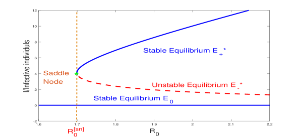
Figure 1: Bistability and saddle-node bifurcation diagram of system (1.1). In this case, $R_{0}^{[sn]}\approx 1.67$. The system displays two stable equilibria $E_{0}$ (the blue solid line at the bottom) and $E_{+}^{*}$ (the above blue curve), indicating bistable behaviour. Here, $\bar{E}$ is the saddle point, where the two equilibria converge and display saddle-node bifurcation. The point $E_{-}^{*}$ (dashed lines) on the bottom half of the curve is unstable, and the point $E_{+}^{*}$ (solid line) on the top half of the curve is stable. Here, $\beta=0.7$ and other parameter values are listed in $(5.1)$.

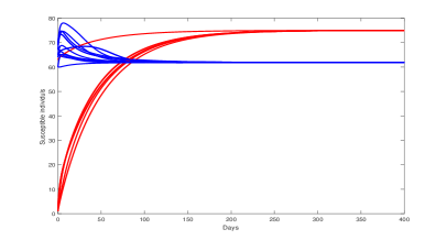
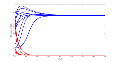
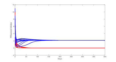
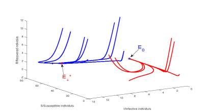
Figure 2: For $R_{0}=2.5$ and other parameter values listed in (5.1), we can see that in the case of different initial values, $S$, $I$ and $R$ converge to either $E_{0}$ or $E_{+}^{*}$. At this interval, the system display two stable equilibria $E_{0}$ and $E_{+}^{*}$, indicating bistable behavior.

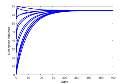
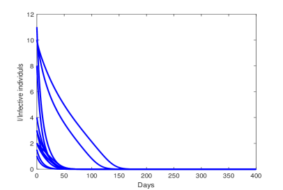
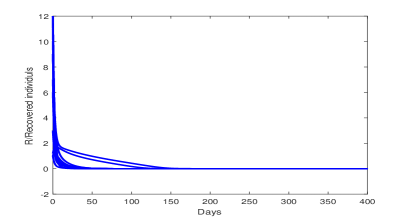
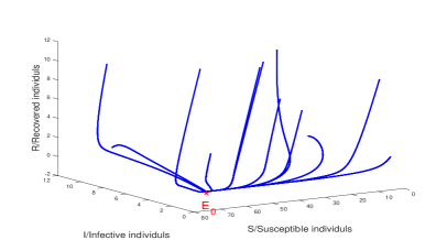
Figure 3: For $R_{0}=1.25$ and other parameter values listed in (5.1), we can see that $S$, $I$ and $R$ converge to $E_{0}$. Here $E_{0}$ is a locally asymptotically stable node.

5.2 Discussion

In this paper, we consider a SIRS model with general nonmonotone and saturated incidence rate and performed mathematical studies. We found that the system displays bistable behaviours. System (1.1) admits an disease-free equilibrium $E_{0}$, and two positive equilibria $E_{+}^{*}$ and $E_{-}^{*}$. We obtain two thresholds $R_{0}=\frac{bk}{\beta d(\mu+d)}$ and $R_{c}=\frac{bk}{\beta d(\mu+d)}-\frac{2}{\beta}\sqrt{\alpha+\frac{k}{d}(1-\frac{\mu\delta}{(\mu+d)(\delta+d)})}$. We find that the system always admits a disease free equilibrium $E_{0}$ which is always asymptotically stable, indicating that there is no infective in the system and all individuals are susceptible. Thus, if there is no disease, then the uninfected state will remain stable for a long time. When $R_{c}>1$ , both $E_{+}^{*}$ and $E_{-}^{*}$ exist, where $E_{+}^{*}$ is locally asymptotically stable and $E_{-}^{*}$ is unstable, which implies the coexistence of susceptible, infective and recovered individuals. Choosing $R_{0}$ as the branching parameter, our investigation implies that if $R_{c}=1$ or $R_{0}=R_{0}^{[sn]}$ system (1.1) undergoes a saddle-node bifurcation. The positive equilibria $E_{+}^{*}$ and $E_{-}^{*}$ collide to each other and system (1.1) has the unique instantaneous endemic equilibrium $\bar{E}$. From the branch diagram in figure 1, we find that when $R_{0}>R_{0}^{[sn]}$, the system has two stable equilibria $E_{+}^{*}$ and $E_{0}$ appear. The system displays bistable behaviour. When $R_{0}<R_{0}^{[sn]}$, the system has only one equilibrium point $E_{0}$, suggesting that infectious diseases will die out eventually.

Castillo-Chavez and Song [12] proposed the backward bifurcation to illustrate that even if the basic reproduction number $R_{0}<1$, disease outbreaks are still possible. The backward bifurcation indicates that the system displays bistable behavior when the bifurcation point $R_{c}<R_{0}<1$.However, when $R_{0}>1$, the system has only one positive equilibrium point, which is stable, and the disease-free equilibrium point is unstable.

In this paper, we investigated a SIRS model with general nonmonotone and saturated incidence rate. We find that (i) the disease-free equilibrium is always stable. (ii) When $1<R_{0}<R_{0}^{[sn]}$, the model does not have positive equilibrium point. (iii) When $R_{0}>R_{0}^{[sn]}$, the system always display bistability behavior. Our investigation implies that non-monotonic incidence is a kind of self-protection behavior of human during the outbreak of a disease. Such self-protection behavior can reduce the basic reproduction number and lead to bistable behavior, i.e., there may or may not be a disease outbreak. Our investigation implies that $R_{0}$ is not the basic reproduction number of the model. We guess that $R_{c}$ may be the basic reproduction number. However, $R_{c}>1$ does not guarantee the outbreak of the disease, which depends on human behavior. How to calculate the basic regeneration number of this model is still an open question.

In other epidemic models with general nonmonotone and saturated incidence rate [13, 14], we also find such bistable phenomenon.

References

[1] H.W. Hethcote, A thousand and epidemic models, in frontiers in theoretical biology, Berlin: Springer-Verlag. (1994).
[2] L. Marcos, R. Jesus, Multiparametric bifurcations for a model in epidemiology, J. Math. Biol. (1996) 21–36.
[3] H.W. Hethcote, The mathematics of infectious disease, SIAM. Review. 42(5.1) (2000) 599–653.
[4] W.O. Kermazk, A.G. McKendrick, A contribution to the mathematical theory of epidemic, Proc. R.
Soc. London. All. 5(1927)700-721.
[5]W. Liu, H.W. Hethcote S.A. Levin, Dynamical behavior of epidemiological models with nonlinear incidence rates, J. Math. Biol. 25 (1987) 359–380.
[6]W. Liu, H.W. Hethcote, S.A. Levin, Influence of nonlinear incidence rates upon the behavior of SIRS epidemiological models, J. Math. Biol. 23 (1986) 187–204.
[7]H.W. Hethcote, P. van den Driessche, Some epidemiological models with nonlinear incidence, J. Math. Biol. 29 (1991) 271–287.
[8] S.G. Ruan, W.D. Wang, Dynamical behavior of an epidemic model with a nonlinear incidence
rate, J. Differential Equations 188 (2003) 135–163.
[9] Y.L. Tang, D.Q. Huang, S.G. Ruan, W.N. Zhang,
Coexistence of limit cycles and homoclinic loops in a SIRS model
with a nonlinear incidence rate, SIAM J. Appl. Math. 69 (2008)
621–639.
[10]J.H. Li, Z.D. Teng, Bifurcations of an SIRS model with
generalized non-monotone incidence rate, Adv. Differ. Equ-Ny.
(2018).
[11]M. Lu, J.C. Huang, S.G. Ruan, P. Yu, Bifurcation analysis of an SIRS epidemic model with a
generalized nonmonotone and saturated incidence rate, J. Differ.
Equations. 267 (2019) 1859–1898.
[12] C. Castillo-Chavez, B.J. Song, Dynamical models of tuberculosis and their applications, Mathematical Biosciences and Engineering, 1 (2004) 361–04.
[13] S.L. Wang, Y.N. Qi, F. Xu, Bistability in SEIS and SEIR models with general nonmonotone
and saturated incidence rate, finished.
[14] S.L. Wang, X.Y. Bai, F. Xu, Bistability in SIQS and SIQR models with general nonmonotone
and saturated incidence rate, finished.