SAT-Encodings for Treecut Width and Treedepth

Abstract

The decomposition of graphs is a prominent algorithmic task with numerous applications in computer science. A graph decomposition method is typically associated with a width parameter (such as treewidth) that indicates how well the given graph can be decomposed. Many hard (even #P-hard) algorithmic problems can be solved efficiently if a decomposition of small width is provided; the runtime, however, typically depends exponentially on the decomposition width. Finding an optimal decomposition is itself an NP-hard task. In this paper we propose, implement, and test the first practical decomposition algorithms for the width parameters treecut width and treedepth. These two parameters have recently gained a lot of attention in the theoretical research community as they offer the algorithmic advantage over treewidth by supporting so-called fixed-parameter algorithms for certain problems that are not fixed-parameter tractable with respect to treewidth. However, the existing research has mostly been theoretical. A main obstacle for any practical or experimental use of these two width parameters is the lack of any practical or implemented algorithm for actually computing the associated decompositions. We address this obstacle by providing the first practical decomposition algorithms.

Our approach for computing treecut width and treedepth decompositions is based on efficient encodings of these decomposition methods to the propositional satisfiability problem (SAT). Once an encoding is generated, any satisfiability solver can be used to find the decomposition. This allows us to leverage the surprising power of todays state-of-the art SAT solvers. The success of SAT-based decomposition methods crucially depends on the used characterisation of the decomposition method, as not every characterisation is suitable for that task. For instance, the successful leading SAT encoding for treewidth is based on a characterisation of treewidth in terms of elimination orderings. For treecut width and treedepth, however, we propose new characterisations that are based on sequences of partitions of the vertex set, a method that was pioneered for clique-width. We implemented and systematically tested our encodings on various benchmark instances, including famous named graphs and random graphs of various density. It turned out that for the considered width parameters, our partition-based SAT encoding even outperforms the best existing SAT encoding for treewidth.

We hope that our encodings—which we will make publicly available—will stimulate the experimental research on the algorithmic use of treecut width and tree depth, and thus will help to bride the gap between theoretical and experimental research. For future work we propose to scale our approach to larger graphs by means of SAT-based local improvement, a method that have been recently shown successful for the width parameters treewidth and branchwidth.

1 Introduction

Graph decompositions have been a central topic in the area of combinatorial algorithms, with applications in many areas of computer science. A graph decomposition method is typically associated with a width parameter that indicates how well the given graph can be decomposed. Tree decompositions, for instance, give rise to the width parameter treewidth. In most cases, finding an optimal decomposition, i.e., one of smallest width, is an NP-hard task, so that for practical purposes one often relies on heuristics that compute suboptimal decompositions. However, there are several reasons why one is interested in optimal decompositions. If the purpose of the decomposition is to facilitate the solution of a hard problem by means of dynamic programming, then a suboptimal decomposition may impose an exponential increase on time and space requirements for the dynamic programming algorithm, and therefore may render the approach infeasible for the instance under consideration. For instance. Kask et al. [22] noted about inference on probabilistic networks of bounded treewidth: “[…] since inference is exponential in the tree-width, a small reduction in tree-width (say even by $1$ or $2$) can amount to one or two orders of magnitude reduction in inference time.” Besides such algorithmic applications, optimal decompositions are also useful for scientific purposes, for instance to evaluate a heuristic method that provides an upper bound on the decomposition width, or to support theoretical investigations by facilitating the construction of gadgets for hardness reductions.

An appealing approach to finding optimal decompositions are SAT-encodings, where one translates a given graph $G$ and an integer $w$ into a propositional formula $F(G,w)$ whose satisfying assignments correspond to a decomposition of $G$ of width at most $w$. The satisfiability of the formula can then be checked by a state-of-the art SAT-solver [27, 28]. This approach was pioneered by Samer and Veith [34] for treewidth. Their encoding was further expanded on in subsequent works [1, 2] and today it still remains one of the most efficient methods for computing optimal tree decompositions. SAT-encodings have also been developed for other graph parameters, including clique-width [18], branchwidth [25], as well as pathwidth and special treewidth [26]. This line of research revealed that the efficiency of the SAT-encoding based approach crucially depends on the underlying characterisation of the considered decompositional parameter. Whereas for treewidth the elimination-ordering based characterisations have been shown to be best suited for SAT-encodings, other decomposition parameters require other characterisations. A very efficient SAT-encoding for clique-width was based on the newly developed partition-based characterisation of clique-width [18]. Partition-based encodings have also been shown to be efficient for other width parameters [25, 26].

In this paper we develop SAT-encodings for the width parameters treecut width and treedepth. These two parameter are both less general than treewidth, i.e., any graph class where either of these two parameters is bounded, is also of bounded treewidth, but there exist graph classes of bounded treewidth where neither of these two parameters are bounded. Neither of the two parameters (treecut width and treedepth) is more general than the other, though. The parameters are of interest as they offer certain algorithmic advantages over treewidth; in particular, they support so-called fixed-parameter algorithms for certain problems that are not fixed-parameter tractable with respect to treewidth (see any of the handbooks on parameterized complexity [7, 5, 10]), as well as having a significantly lower parameter dependency than treewidth for certain problems [13, 8].

So far, both parameters have mainly been the subject of theoretical investigations. By our encodings we provide the first practical methods for computing the associated decompositions and therefore provide a first step of bridging theoretical with experimental research.

1.1 Treecut Width

The parameter treecut width was introduced by Wollan [36]. Treecut width is an edge-separator based decompositional parameter whose relationship to the fundamental notion of graph immersions is analogous to the relationship between treewidth and graph minors [29]. Kim et al. [23] gave a linear time 2-approximation algorithm for treecut width, however, such an error factor is prohibitive for practical use. Ganian et al. [14, 15] provided the first algorithmic results for treecut width, and pointed out that several problems that are not fixed-parameter tractable for the parameter treewidth are fixed-parameter tractable for the parameter treecut width.

Given that treecut width arguably has the most complicated and unintuitive characterisation among all studied width parameters, our first step was to find a way to simplify the definition of treecut width. Such a simplification has recently been proposed by Kim et al. [23], showing that the definition of treecut decompositions becomes significantly more manageable on $3$-edge-connected graphs and that computing decompositions for general graphs can be reduced to the $3$-edge-connected case. Using this simpler definition together with an explicit preprocessing procedure for general graphs (presented in Section 2.3), we introduce a SAT-encoding for $3$-edge-connected graphs based on a partition-based characterisation of treecut width in Section 3. As our experiments show, the encoding performs extraordinary well; outperforming even our arguably much simpler encoding for treedepth and the current best-performing SAT-encoding for treewidth [1, 2, 34].

1.2 Treedepth

The parameter treedepth was introduced by Nešetřil and Ossona de Mendez [30] in the context of their graph sparsity project [31]. This parameter has been shown to have algorithmic applications for a number of problems where treewidth cannot be used. For instance, Gutin et al. [17] showed that the Mixed Chinese Postman problem is fixed-parameter tractable for treedepth, but W[1]-hard for treewidth and even pathwidth. Several further algorithmic results on treedepth have been presented recently by Iwata et al. [21], Koutecký et al. [24], Ganian and Ordyniak [16], and Gajarský and Hliněný [12]. Exact algorithms for computing treedepth are known, e.g., the problem is known to be fixed-parameter tractable [33] and can be solved slightly faster than $\mathcal{O}(2^{n})$ [11], however, until now no implementation of an exact algorithm for treedepth was available.

We introduce and implement two SAT-encodings for treedepth. The first one explicitly guesses the tree-structure of a treedepth decomposition and the second one is based on a novel partition-based characterisation of treedepth. Since the partition-based encoding greatly outperformed our first encoding, we mostly focus on the partition-based encoding. The experimental results for our partition-based encoding are very promising, showing an extraordinarily good performance on sparse classes of graphs such as paths, cycles, and complete binary trees. We also introduce three novel preprocessing and symmetry breaking procedures for treedepth.

1.3 Related Work

We have already mentioned the successful application of SAT-encodings for graph decompositions above [1, 2, 18, 25, 34]. At this juncture we would like to briefly give some further context on SAT-encodings. While every problem in NP admits a polynomial-time SAT-encoding, it is well known that different encodings can behave quite differently in practice [32]. There are some formal criteria which indicate whether an encoding will behave well or not. However, only by an experimental evaluation one can see what really works well and what does not [4]. For instance, while encoding size is certainly a factor to take into consideration, larger encodings can work better if they allow a fast propagation of conflicts, so that the power of state-of-the art SAT-solvers which are based on the conflict-driven clause learning paradigm (CDCL) [27, 28] can be harvested. SAT-encodings are not only useful for the solution of hard combinatorial problems in industry, such as the verification of hardware and software [3], but are increasingly often used in the context of Combinatorics, for instance in the context of Ramsey Theory [37]. A very recent highlight is the celebrated solution to the Pythagorean Triples Problem [20, 19].

Lastly, we would like to mention that developing partition-based encodings comes with challenges that are specific to each width parameter, as it almost always requires the development of a novel characterization that is compatible with such an encoding. Indeed, the existence of such an encoding for the probably most prominent width parameter, treewidth, remains open.

2 Preliminaries

We use $[i]$ to denote the set $\{0,1,\dots,i\}$. A weak partition of a set $S$ is a set $P$ of nonempty subsets of $S$ such that any two sets in $P$ are disjoint; if additionally $S$ is the union of all sets in $P$ we call $P$ a partition. The elements of $P$ are called equivalence classes. Let $P,P^{\prime}$ be partitions of $S$. Then $P^{\prime}$ is a refinement of $P$ if for any two elements $x,y\in S$ that are in the same equivalence class of $P^{\prime}$ are also in the same equivalence class of $P$ (this entails the case $P=P^{\prime}$).

2.1 Formulas and Satisfiability

We consider propositional formulas in Conjunctive Normal Form (CNF formulas, for short), which are conjunctions of clauses, where a clause is a disjunction of literals, and a literal is a propositional variable or a negated propositional variable. A CNF formula is satisfiable if its variables can be assigned true or false, such that each clause contains either a variable set to true or a negated variable set to false. The satisfiability problem (SAT) asks whether a given formula is satisfiable.

We will now introduce a few general assumptions and notation that is shared among our encodings. Namely, for our encodings we will assume that we are given an undirected graph $G=(V,E)$ and an integer $\omega$, which represents the width that we are going to test. Moreover, we will assume that the vertices of $G$ are numbered from $1$ to $n$ and similarly the edges are numbered from $1$ to $m$.

For the counting part of our encodings we will employ the sequential counter approach [34] since this approach has turned out to provide the best results in our setting. To illustrate the idea behind the sequential counter consider the case that one is given a set $S$ of (propositional) variables and one needs to restrict the number of variables in $S$ that are set to true to be at most some integer $k$. For convenience, we refer to the elements in $S$ using the numbers from $1$ to $|S|$. In this case one introduces a counting variable $\mathsf{\#}(s,j)$ for every $s\in S$ and $j$ with $1\leq j\leq k$, which is true whenever there are at least $j$ variables in $\{\,s^{\prime}\mid s^{\prime}\leq s\text{ and }s,s^{\prime}\in S\,\}$ that are set to true. Then this can be ensured using the following clauses. A clause $\neg s\lor\mathsf{\#}(s,1)$ for every $s\in S$, a clause $\neg\mathsf{\#}(s-1,j)\lor\mathsf{\#}(s,j)$ for every $s\in S$ and $j$ with $s>1$ and $1\leq j\leq k$, a clause $\neg s\lor\neg\mathsf{\#}(s-1,j-1)\lor\mathsf{\#}(s,j)$ for every $s\in S$ and $j$ with $s>1$ and $1<j\leq k$, and a clause $\neg s\lor\neg\mathsf{\#}(s-1,k)$ for every $s\in S$ with $s>1$. This adds at most $\mathcal{O}(|S|k)$ variables and clauses to the original formula.

2.2 Graphs

We use standard terminology for graph theory, see for instance [6]. All graphs in this paper are undirected and may contain multiedges. Given a graph $G$, we let $V(G)$ denote its vertex set and $E(G)$ its (multi-) set of edges. The (open) neighbourhood of a vertex $x\in V(G)$ is the set $\{y\in V(G):xy\in E(G)\}$ and is denoted by $N_{G}(x)$. For a vertex subset $X$, the neighbourhood of $X$ is defined as $\bigcup_{x\in X}N_{G}(x)\setminus X$ and denoted by $N_{G}(X)$; we drop the subscript if the graph is clear from the context. For a vertex set $A$ (or edge set $B$), we use $G-A$ ($G-B$) to denote the graph obtained from $G$ by deleting all vertices in $A$ (edges in $B$), and we use $G[A]$ to denote the subgraph induced on $A$, i.e., $G-(V(G)\setminus A)$. Let $T$ be a rooted tree and $t\in V(T)$. We write $T_{t}$ to denote the subtree of $T$ rooted in $t$, i.e., the component of $T\setminus\{\{t,p\}\}$ containing $t$, where $p$ is the parent of $t$ in $T$. We denote by $\textup{h}_{T}(t)$, the height of $t$ in $T$, i.e., the length of the path between the root of $T$ and $t$ in $T$ plus one, and we denote by $\textup{h}(T)$ the height of $T$, i.e., the maximum of $\textup{h}_{T}(t^{\prime})$ over all $t^{\prime}\in V(T)$. Let $G$ be a graph. We say that two vertices $u$ and $v$ of $G$ are $3$-edge-connected in $G$ if there are at least $3$ pairwise edge disjoint paths between $u$ and $v$ in $G$. We say a subset $C$ of $V(G)$ is a $3$-edge-connected component of $G$ if every pair of distinct vertices in $C$ is $3$-edge-connected and $C$ is maximal w.r.t. this property. For a graph $G$ and a subset $V^{\prime}\subseteq V(G)$, we denote by $\delta_{G}(V^{\prime})$ the (multi-)set of edges of $G$ having one endpoint in $V^{\prime}$ and one endpoint in $V(G)\setminus V^{\prime}$ and omit the subscript $G$ if it can be inferred from the context. An apex vertex is a vertex adjacent to all other vertices in the graph.

2.3 Treecut Width

The notion of treecut width and treecut decomposition was originally introduced for general graphs [29, 36]. Here we use a simpler definition, which allows for an easier encoding, and only applies for $3$-edge-connected graphs. Using known results [23], we will then show that the treecut width for general graphs can be defined in terms of the treecut widths of its $3$-edge-connected components.

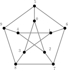
Figure 1: A width-$6$ treedepth decomposition (top right) and a width-$5$ treecut decomposition (bottom) of the Petersen graph (top left). The treecut decomposition lists the adhesion (left value) and torso-width (right value) of each node.

Let $G$ be a $3$-edge connected undirected graph (possibly with multi-edges and loops). A treecut decomposition of $G$ is a pair $(T,\chi)$, where $T$ is a rooted tree and $\chi:V(T)\rightarrow 2^{V(G)}$ such that $\{\,\chi(t)\mid t\in V(T)\,\}$ forms a near partition of $V(G)$, i.e., a partition of $V(G)$ allowed to contain the empty set. For a subgraph $T^{\prime}$ of $T$, we denote by $\chi(T^{\prime})$ the set $\bigcup_{t\in V(T^{\prime})}\chi(t)$. Let $t\in V(T)$. We denote by $V_{t}$ the set $\chi(T_{t})$. The adhesion of $t$, denoted by $\mathsf{ad}(t)$, is the (multi-)set $\delta_{G}(V_{t})$. Moreover, the torsowidth of $t$, denoted by $\mathsf{tor}(t)$, is equal to $|\chi(t)|$ plus the number of neighbours of $t$ in $T$. The width of $(T,\chi)$ is the maximum width of any of its nodes $t\in V(T)$, which in turn is equal to $\max\{|\mathsf{ad}(t)|,\mathsf{tor}(t)\}$. The height of $(T,\chi)$ is simply the height of $T$. Finally, the treecut width of $G$, denoted by $\mathsf{tcw}(G)$, is the minimum width of any of its treecut decompositions. Figure 1 illustrates a treecut decomposition for the Peterson graph.

The following lemma shows that if a graph is not $3$-edge-connected, then it can be modified and split into parts in such a way that its treecut width can be computed from the treecut width of the (modified) parts. Since a recursive application of this lemma eventually results in $3$-edge-connected graphs, the lemma allows us to apply our encoding for $3$-edge-connected graphs to arbitrary graphs.

Lemma 2.1

Let $G$ be a multigraph, $C$ be a minimal cut of size at most two resulting in the partition $(A,B)$ of $V(G)$, and let $A_{C}$ and $B_{C}$ be the endpoints of the edges in $C$ in $A$ and $B$, respectively. If $C$ contains two edges and $|A_{C}|=|B_{C}|=1$, then $\mathsf{tcw}(G)=\max\{2,\mathsf{tcw}(G[A]),\mathsf{tcw}(G[B])\}$. Otherwise, $\mathsf{tcw}(G)=\max\{\mathsf{tcw}(G_{A}),\mathsf{tcw}(G_{B})\}$, where $G_{A}$ ($G_{B}$) is obtained from $G[A]$ ($G[B]$) after adding an edge between the vertices in $A_{C}$ ($B_{C}$); note that an edge is only added if $|A_{C}|=2$ or $|B_{C}|=2$, respectively.

• The proof is closely based on the ideas in [23, Section 3]. Namely, in the case that $C$ does not contain two edges sharing the same endpoints, the proof follows immediately from [23, Lemma 3 and 4]. Moreover, if $C$ contains two edges sharing the same endpoints, say $a\in A$ and $b\in B$, it follows from [23, Lemma 3] that $\mathsf{tcw}(G)=\max\{\mathsf{tcw}(G[A\cup\{b\}]),\mathsf{tcw}(G[B\cup\{a\}])$. Moreover, using the definition of treecut width for arbitrary graphs and recalling that $b$ has precisely $2$ neighbours in $A$ (and similarly $a$ has precisely $2$ neighbours in $B$), it is then easy to see that $\mathsf{tcw}(G[A\cup\{b\}])=\max\{2,\mathsf{tcw}(G[A])\}$ and similarly $\mathsf{tcw}(G[B\cup\{a\}])=\max\{2,\mathsf{tcw}(G[B])\}$, from which the lemma follows. More precisely, this follows immediately by observing that (1) $\mathsf{tcw}(G[\{a,b\}])=2$ and (2) a treecut decomposition $(T,\chi)$ of $G[A]$ ($G[B]$) of width $w$ can be turned into a treecut decomposition of $G[A\cup\{b\}]$ ($G[B\cup\{a\}]$) of width $\max\{2,w\}$ by adding a leaf $l$ containing $b$ ($a$) as a leaf to an arbitrary node of $T$. Note that $l$ has torsowidth at most $2$ and the torsowidth of the neighbor of $l$ in $T$ is not increased; to see this one needs to use the definition of treecut width on general graphs and the fact that $l$ is a thin node [14]. $\blacksquare$

We also give the known relations between treecut width, treewidth, and maximum degree.

Lemma 2.2 ([14, 29, 36])

For every graph $G$, $\mathsf{tw}(G)\leq 2\mathsf{tcw}(G)^{2}+3\mathsf{tcw}(G)$ and $\mathsf{tcw}(G)\leq 4\Delta(G)\cdot\mathsf{tw}(G)$, where $\Delta(G)$ and $\mathsf{tw}(G)$ denote the maximum degree and treewidth of $G$, respectively.

We close this section by showing explicit values of treecut width for complete graphs ($K_{n}$) and complete bipartite graphs ($K_{n,n}$), which we later employ to verify the correctness of our encoding. For the proofs we will assume w.l.o.g. that a treecut decomposition $(T,\chi)$ does not contain unnecessary nodes, i.e., $\chi(l)\neq\emptyset$ if $l$ has at most one child in $T$.

Lemma 2.3

For every $n\geq 4$, $\mathsf{tcw}(K_{n})=n$.

• First, note that $\mathsf{tcw}(K_{n})\leq n$ since there is a trivial treecut decomposition of width $n$. So, assume for a contradiction that there exists a treecut decomposition $(T,\chi)$ of $K_{n}$ of width smaller than $n$; without loss of generality, we assume that $\chi(t)\neq\emptyset$ for each leaf $t$ of $T$, and similarly $\chi(t^{\prime})\neq\emptyset$ for each parent $t^{\prime}$ of a single leaf in $T$. Since $n\geq 4$, in order not to exceed the bound on the width due to adhesion, for each edge $e$ of $T$ it must hold that one tree in $T-e$ must contain a single node (i.e., a leaf) $u$ and $|\chi(u)|=1$. From this it follows that $T$ must be a star (with center $r$). However, since the torsowidth of $r$ is equal to $|\chi(r)|$ plus the number of leaves (each representing a single vertex of $K_{n}$), we see that $\mathsf{tor}(r)=n$, a contradiction. $\blacksquare$

Lemma 2.4

For every $n\geq 3$, $\mathsf{tcw}(K_{n,n})=2n-2$.

• Let $V(K_{n,n})=\{a_{1},\dots,a_{n},b_{1},\dots,b_{n}\}$ and $E(K_{n,n}=\{\,a_{i}b_{j}\mid i,j\in[n]\,\}$. We obtain a treecut decomposition of $K_{n,n}$ of width $2n-2$ as follows: $T^{\prime}$ is a star with center $r$ and leaves $t_{1},\dots,t_{n}$, where $\chi^{\prime}(r)=\emptyset$ and $\chi^{\prime}(t_{i})=\{a_{i},b_{i}\}$ for all $i\in[n]$.

  Now, assume for a contradiction that there exists a treecut decomposition $(T,\chi)$ of width smaller than $2n-2$. As before, we assume that $\chi(t)\neq\emptyset$ for each leaf $t$ of $T$, and similarly $\chi(t^{\prime})\neq\emptyset$ for each parent $t^{\prime}$ of a single leaf in $T$. Since $n\geq 3$, in order not to exceed the bound on the width due to adhesion, for each edge $e$ of $T$ it must hold that one tree in $T-e$ must contain a single node (i.e., a leaf) $u$ and $|\chi(u)|=1$. As before, from this it follows that $T$ must be a star (with center $r$). However, since the torsowidth of $r$ is equal to $|\chi(r)|$ plus the number of leaves (each representing a single vertex of $K_{n}$), we see that in fact $\mathsf{tor}(r)=2n$, a contradiction. $\blacksquare$

2.4 Treedepth

The second decompositional parameter for which we will introduce a SAT-encoding is treedepth [31]. Treedepth is closely related to treewidth, and the structure of graphs of bounded treedepth is well understood [31]. A useful way of thinking about graphs of bounded treedepth is that they are (sparse) graphs with no long paths.

The treedepth of an undirected graph $G$, denoted by $\mathsf{td}(G)$, is the smallest natural number $k$ such that there is an undirected rooted forest $F$ with vertex set $V(G)$ of height at most $k$ for which $G$ is a subgraph of $C(F)$, where $C(F)$ is called the closure of $F$ and is the undirected graph with vertex set $V(F)$ having an edge between $u$ and $v$ if and only if $u$ is an ancestor of $v$ in $F$. A forest $F$ for which $G$ is a subgraph of $C(F)$ is also called a treedepth decomposition, whose depth is equal to the height of the forest. Informally a graph has treedepth at most $k$ if it can be embedded in the closure of a forest of height $k$. Note that if $G$ is connected, then it can be embedded in the closure of a tree instead of a forest. A treedepth decomposition of the Peterson graph is illustrated in Figure 1.

We conclude with some useful facts about treedepth.

Lemma 2.5 ([31])

For every graph $G$, $\mathsf{tw}(G)\leq\mathsf{td}(G)$ and $\mathsf{pw}(G)\leq\mathsf{td}(G)$, where $\mathsf{pw}(G)$ is the pathwidth of $G$.

3 Treecut Width

In this section we will introduce our encoding for treecut width. The encoding is based on a different characterisation of treecut width, one that is well-suited for SAT-encodings.

3.1 Partition-Based Formulation

Here we present a partition-based characterisation of treecut width, in terms of what we call derivations, which is well-suited for an encoding into SAT. Let $G$ be a graph. A derivation $\mathcal{P}$ of $G$ of length $l$ is a sequence $(P_{1},\dotsc,P_{l})$ of weak partitions of $V(G)$ such that:

• $P_{1}=\emptyset$ and $P_{l}=\{\{V(G)\}\}$ and

• for every $i\in\{1,\dots,l\}$, $P_{i}$ is a refinement of $P_{i+1}$.

We will refer to $P_{i}$ as the $i$-th level of the derivation $\mathcal{P}$ and we will refer to elements in $\bigcup_{1\leq i\leq l}P_{i}$ as sets of the derivation. Let $p\in P_{i}$ for some level $i$ with $1\leq i\leq l$. We say that a set $c\in P_{i-1}$ is a child of $p$ at level $i$ if $c\subseteq p$ and denote by $\mathsf{c}_{\mathcal{P}}^{i}(p)$ the set of all children of $p$ at level $i$. Moreover, we denote by $\chi_{\mathcal{P}}^{i}(p)$ the set $p\setminus(\bigcup_{c\in\mathsf{c}_{\mathcal{P}}^{i}(p)}c)$. Then the width of $p$ at level $i$ is equal to the maximum of $|\delta_{G}(p)|$ and $\mathsf{tor}_{\mathcal{P}}^{p}(i)$, where $\mathsf{tor}_{\mathcal{P}}^{p}(i)$ is equal to $|\chi_{\mathcal{P}}^{i}(p)|+|\mathsf{c}_{\mathcal{P}}^{i}(p)|+1$ if $i\neq l$ and equal to $|\chi_{\mathcal{P}}^{i}(p)|+|\mathsf{c}_{\mathcal{P}}^{i}(p)|$ otherwise. We will show that any treecut decomposition can be transformed into a derivation of the same width, and vice versa. The following example illustrates the close connection between treecut decompositions and derivations.

Example: The treecut decomposition given in Fig. 1 of the Petersen graph can be translated into the derivation $\mathcal{P}=(P_{1},\dotsc,P_{3})$ defined by:

$P_{1}=\emptyset$, $P_{2}=\Big{\{}\big{\{}0,5,6\big{\}},\big{\{}1\big{\}},\big{\{}2,4,7\big{\}},\big{\{}3,8,9\big{\}}\Big{\}}$,
$P_{3}=\Big{\{}\big{\{}0,1,2,3,4,5,6,7,8,9\big{\}}\Big{\}}$.

As can be verified easily, the width of $\mathcal{P}$ is equal to $5$.

We show that derivations provide an alternative characterisation of treecut decompositions.

Theorem 3.1

Let $G$ be a graph and $\omega$ and $d$ two integers. $G$ has a treecut decomposition of width at most $\omega$ and height at most $d$ if and only if $G$ has a derivation of width at most $\omega$ and length at most $d+1$.

• Let $(T,\chi)$ be a treecut decomposition of $G$ of width at most $\omega$ and height at most $d$; without loss of generality, we assume that $\chi(t)\neq\emptyset$ for each leaf $t$ of $T$. It is immediate from the definitions that $\mathcal{P}=(P_{1},\dotsc,P_{\textup{h}(T)+1})$ such that $P_{1}=\emptyset$ and $P_{i}=\{\,V_{t}\mid t\in V(T)\land\textup{h}_{T}(t)=\textup{h}(T)-i+2\,\}$ for every $i$ with $2\leq i\leq\textup{h}(T)+1$ is a derivation of $G$ with width at most $\omega$ and length at most $d+1$.

  Towards showing the converse, let $\mathcal{P}=(P_{1},\dotsc,P_{l})$ be a derivation of $G$ with width at most $\omega$. It is immediate from the definitions that $(T,\chi)$ such that:

  • $T$ is the tree with a vertex for every pair $(p,i)$ such that $p\in P_{i}$ having an edge between $(c,i-1)$ and $(p,i)$ if $c$ is a child of $p$ at level $i$, and

  • $\chi((p,i))=\chi_{\mathcal{P}}^{i}(p)$ for every level $i$ and $p\in P_{i}$

  is a treecut decomposition of $G$ with width at most $\omega$ and height at most $d-1$. $\blacksquare$

3.2 Encoding

Let $G$ be a graph with $m$ edges and $n$ vertices, and let $\omega$ and $d$ be positive integers. We will assume that the vertices of $G$ are represented by the numbers from $1$ to $n$ and the edges of $G$ by the numbers from $1$ to $m$. The aim of this section is to construct a formula $F(G,\omega,d)$ that is satisfiable if and only if $G$ has a derivation of width at most $\omega$ and length at most $d$. Because of Theorem 3.1 (after setting $d$ to $n$) it holds that $F(G,\omega,d)$ is satisfiable if and only if $G$ has treecut width at most $\omega$. To achieve this aim we first construct a formula $F(G,d)$ such that every satisfiable assignment encodes a derivation of length at most $d$ and then we extend this formula by adding constrains that restrict the width of the derivation to $\omega$.

3.2.1 Encoding of a Derivation

The formula $F(G,d)$ uses the following variables. A set variable $\mathsf{s}(u,v,i)$, for every $u,v\in V(G)$ with $u\leq v$ and every $i$ with $1\leq i\leq d$. Informally, $\mathsf{s}(u,v,i)$ is true whenever $u$ and $v$ are contained in the same set at level $i$ of the derivation. Note that $\mathsf{s}(u,u,i)$ is true whenever $u$ is contained in some set at level $i$. Furthermore, the formula contains a leader variable $\mathsf{l}(u,i)$, for every $u\in V(G)$ and every $i$ with $1\leq i\leq d$. Informally, the leader variables will be used to uniquely identify the sets at each level of a derivation (using the smallest vertex contained in the set as the unique identifier), i.e., $\mathsf{l}(u,i)$ is true whenever $u$ is the smallest vertex in a set at level $i$ of the derivation.

We now describe the clauses of the formula. The following clauses ensure (D1) and (D2).

$\neg\mathsf{s}(u,v,1)\wedge\mathsf{s}(u,v,d)$ for $u,v\in V(G)$, $u\leq v$

$\neg\mathsf{s}(u,v,i)\vee\mathsf{s}(u,v,i+1)$

******* for $u,v\in V(G)$, $u\leq v$, $1\leq i<d$

The following clauses ensure that if a vertex $v$ is in some set with at least one other vertex at level $i$, then $\mathsf{s}(v,v,i)$ is true.

$(\neg\mathsf{s}(u,v,i)\vee\mathsf{s}(u,u,i))\wedge(\neg\mathsf{s}(u,v,i)\vee\mathsf{s}(v,v,i))$

******* for $u,v\in V(G)$, $u<v$, $2\leq i\leq d$

The following clauses ensure that the relation of being in the same set is transitive.

$(\neg\mathsf{s}(u,v,i)\vee\neg\mathsf{s}(u,w,i)\vee\mathsf{s}(v,w,i))$

$\wedge(\neg\mathsf{s}(u,v,i)\vee\neg\mathsf{s}(v,w,i)\vee\mathsf{s}(u,w,i))$

$\wedge(\neg\mathsf{s}(u,w,i)\vee\neg\mathsf{s}(v,w,i)\vee\mathsf{s}(u,v,i))$

******* for $u,v,w\in V(G)$, $u<v<w$, $1\leq i\leq d$

The following clauses ensure that $\mathsf{l}(u,i)$ is true if and only if $u$ is the smallest vertex contained in some set at level $i$ of a derivation.

(A)  $(\mathsf{l}(u,i)\vee\neg\mathsf{s}(u,u,i)\vee\bigvee\limits_{v\in V(G),v<u}\mathsf{s}(v,u,i))\wedge$

(B)  $(\neg\mathsf{l}(u,i)\vee\mathsf{s}(u,u,i))\wedge\bigwedge\limits_{v\in V(G),v<u}(\neg{\mathsf{l}}(u,i)\vee$

(*)  $\neg\mathsf{s}(v,u,i))$

x for $u\in V(G)$, $1\leq i\leq d$

Part $A$ ensures that if $u$ is contained in some set at level $i$ and no vertex smaller than $u$ is contained in a set with $u$ at level $i$, then $u$ is a leader. Part $B$ ensures that if $u$ is a leader at level $i$, then $u$ is contained in some set at level $i$ and furthermore no vertex smaller than $u$ at level $i$ is in the same set as $u$. The formula $F(H,d)$ contains at most $\mathcal{O}(n^{2}d)$ variables and $\mathcal{O}(n^{3}d)$ clauses.

3.2.2 Encoding of a Derivation of Bounded Width

Next, we describe how $F(G,d)$ can be extended to restrict the width of the derivation. Towards this aim we first need new variables allowing us to define adhesion and torsowidth. Namely, for every $u\in V(G)$, $e\in E(G)$ such that at least one of the endpoints of $e$ is larger or equal to $u$, and $i\in\{2,\dotsc,d-1\}$, we use the variable $\textsf{ad}(u,e,i)$, which will be true if $u$ is a leader of some set $V^{\prime}$ at level $i$ and $e\in\delta_{G}(V^{\prime})$. This is ensured by the following clauses.

$\neg\mathsf{l}(u,i)\vee\neg\mathsf{s}(u,v,i)\vee\mathsf{s}(u,w,i)\vee\textsf{ad}(u,e,i)$

x for $u,v,w\in V(G)$, $e=\{v,w\}\in E(G)$, $u\leq v$,
x $u\leq w$, and $1<i<d$.

$\neg\mathsf{l}(u,i)\vee\neg\mathsf{s}(u,v,i)\vee\textsf{ad}(u,e,i)$

x for $u,v,w\in V(G)$, $e=\{v,w\}\in E(G)$, $u\leq v$,
x $w<u$, and $1<i<d$.

Note that we do not require the reverse direction here since the sole purpose of the variables $\textsf{ad}(u,e,i)$ is to ensure that the adhesion never exceeds the width.

Towards defining torsowidth, we introduce the variable $\textsf{tor}(u,v,i)$ for every $u,v\in V(G)$, $u\leq v$, and $1\leq i\leq d$, which will be true, whenever $u$ is a leader of a set $V^{\prime}$ at level $i$, $v$ is in $V^{\prime}$, and either $v$ is a leader at level $i-1$, or $v$ is not in a set at level $i-1$. This is ensured by the following clauses.

$\neg\mathsf{l}(u,i)\vee\neg\mathsf{s}(u,v,i)\vee\neg\mathsf{l}(v,i-1)\vee\textsf{tor}(u,e,i)$

** for $u,v\in V(G)$, $u\leq v$, and $2<i\leq d$

$\neg\mathsf{l}(u,i)\vee\neg\mathsf{s}(u,v,i)\vee\neg\mathsf{s}(v,v,i-1)\vee\textsf{tor}(u,e,i)$

** for $u,v\in V(G)$, $u\leq v$, and $1<i\leq d$

Note that after adding the above variables and clauses defining adhesion and torsowidth, our formula has at most at most $\mathcal{O}(n^{2}d+nmd)$ variables and $\mathcal{O}(n^{3}d)$ clauses.

Finally, we use the sequential counter introduced in Section 2.1 to ensure that both the adhesion as well as the torsowidth do not exceed the given width. Namely, for every $u\in V(G)$ and $i$ with $1<i<d$, we ensure that the number of variables in $\{\,\textsf{ad}(u,e,i)\mid e\in E(G)\,\}$ that are set to true does not exceed $\omega$. Similarly for every $u\in V(G)$ and $i$ with $1<i<d$, we ensure that the number of variables in $\{\,\textsf{tor}(u,v,i)\mid v\in V(G)\land u\leq v\,\}$ that are set to true does not exceed $\omega-1$ and that the number of variables in $\{\,\textsf{tor}(u,v,d)\mid v\in V(G)\land u\leq v\,\}$ does not exceed $\omega$.

This completes the construction of $F(G,\omega,d)$. By construction, $F(G,\omega,d)$ is satisfiable if and only $G$ has a derivation of width at most $\omega$ and length at most $d$. Due to Theorem 3.1, we obtain:

Theorem 3.2

The formula $F(G,\omega,d)$ is satisfiable if and only if $G$ has a treecut decomposition of width at most $\omega$ and depth at most $d$. Moreover, such a treecut decomposition can be constructed from a satisfying assignment of $F(G,\omega,d)$ in linear time w.r.t. the number of variables of $F(G,\omega,d)$.

4 Treedepth

In this section we introduce a SAT-encoding for treedepth, which is also based on partitions. We also developed an encoding for treedepth that is based on guessing the tree of the treedepth decomposition, however, the encoding has, to our surprise, performed much worse than the partition-based encoding. Namely, the encoding, which we introduce for completeness in Section 4.3, only terminated on 17 out of the 39 famous graphs.

4.1 Partition-Based Formulation

Let $G$ be a graph. We will base our definition of derivations for treedepth on the derivations defined for treecut width in Section 3.1. A derivation $\mathcal{P}$ of $G$ of length $l$ is a sequence $(P_{1},\dotsc,P_{l})$ of weak partitions of $V(G)$ satisfying (D1) and (D2) and additionally the following properties:

• for every $p\in P_{i}$, $|\chi_{\mathcal{P}}^{i}(p)|\leq 1$, and

• for every edge $\{u,v\}\in E(G)$, there is a $p\in P_{i}$ such that $\{u,v\}\subseteq p$ and $\chi_{\mathcal{P}}^{i}(p)\cap\{u,v\}\neq\emptyset$.

It will be useful to recall the notions defined for derivations in Section 3.1. We will show that any treedepth decomposition of depth $\omega$ can be transformed into a derivation of length $\omega+1$, and vice versa. The following example illustrates the connection between treedepth and such derivations.

Example: The treedepth decomposition given in Fig. 1 of the Petersen graph can be translated into the derivation $\mathcal{P}=(P_{1},\dotsc,P_{7})$ defined by:

$P_{1}=\emptyset$, $P_{2}=\Big{\{}\big{\{}4\big{\}},\big{\{}8\big{\}},\big{\{}5\big{\}}\Big{\}}$,

$P_{3}=\Big{\{}\big{\{}2,4\big{\}}\big{\{}3,8\big{\}},\big{\{}5,6\big{\}}\Big{\}}$,

$P_{4}=\Big{\{}\big{\{}1,2,3,4,5,6,8\big{\}}\Big{\}}$,

$P_{5}=\Big{\{}\big{\{}0,1,2,3,4,5,6,8\big{\}}\Big{\}}$

$P_{6}=\Big{\{}\big{\{}0,1,2,3,4,5,6,7,8\big{\}}\Big{\}}$,

$P_{7}=\Big{\{}\big{\{}0,1,2,3,4,5,6,7,8,9\big{\}}\Big{\}}$.

The next theorem shows that such derivations provide an alternative characterisation of treedepth.

Theorem 4.1

Let $G$ be a connected graph and $\omega$ an integer. $G$ has a treedepth decomposition of depth at most $\omega$ if and only if $G$ has a derivation of length at most $\omega+1$.

• Let $T$ be a treedepth decomposition of $G$. It is immediate from the definitions that $\mathcal{P}=(P_{1},\dotsc,P_{\textup{h}(T)+1})$ such that $P_{1}=\emptyset$ and $P_{i}=\{\,V(T_{t})\mid t\in V(T)\land\textup{h}_{T}(t)=\textup{h}(T)-i+2\,\}$ for every $i$ with $2\leq i\leq\textup{h}(T)+1$ is a derivation of $G$ whose length is equal to the height of $T$ plus 1.

  Towards showing the converse, let $\mathcal{P}=(P_{1},\dotsc,P_{l})$ be a derivation of $G$.Note first that w.l.o.g. we can assume that $\chi_{\mathcal{P}}^{i}(p)\neq\emptyset$ for every $i$ with $1\leq i\leq l$ and $p\in P_{i}$; this is because if this is not the case we can replace $p$ in $P_{i}$ with all its children in $P_{i-1}$. Note also that for every $v\in V(G)$, there is exactly one $p\in P_{i}$ such that $\{v\}=\chi_{\mathcal{P}}^{i}(p)$, which we will call the set of $\mathcal{P}$ introducing $v$. Let $T$ be the tree with vertex set $V(G)$ having an edge between $u$ and $v$, whenever the set introducing $u$ is a child of the set introducing $v$ or vice versa and let $\chi_{der}^{l}(r)$ with $r\in P_{l}$ be the root of $T$. It is straightforward to verify that $T$ is a treedepth decomposition of $G$ with depth at most $l-1$. $\blacksquare$

4.2 Encoding of a Derivation

Here we construct the formula $F(G,\omega)$ that is satisfiable if and only if $G$ has a derivation of length at most $\omega$, which together with Theorem 4.1 implies that $G$ has treedepth $\omega-1$. Since we are again using derivations, the formula $F(G,\omega)$ is relatively similar to the formula $F(G,d)$ introduced in Section 3.2.1. In particular, we again have a set variable $\mathsf{s}(u,v,i)$, for every $u,v\in V(G)$ with $u\leq v$ and every $i$ with $1\leq i\leq\omega$, which has the same semantics as before. It also contains all the clauses introduced in Section 3.2.1 apart from the clauses restricting the leader variables. Additionally, we have the following clauses, which ensure that (D3) holds, i.e., that there is at most one vertex in $\chi_{\mathcal{P}}^{i}(p)$.

$\neg\mathsf{s}(u,v,i)\vee\mathsf{s}(u,u,i-1)\vee\mathsf{s}(v,v,i-1)$

*** for all $u,v\in V$, $u<v$, and $2\leq i\leq\omega$

Finally, the following clauses ensure (D4).

$\neg\mathsf{s}(u,u,i)\vee\neg\mathsf{s}(v,v,i)\vee\mathsf{s}(u,u,i-1)\vee\mathsf{s}(u,v,i)$

$\neg\mathsf{s}(u,u,i)\vee\neg\mathsf{s}(v,v,i)\vee\mathsf{s}(v,v,i-1)\vee\mathsf{s}(u,v,i)$

*** for $uv\in E$, $u<v$, and $2\leq i\leq\omega$

This completes the construction of the formula $F(G,\omega)$, which has at most $\mathcal{O}(n^{2})$ variables and at most $\mathcal{O}(n^{3}\omega)$ clauses. By construction, $F(G,\omega)$ is satisfiable if and only $G$ has a derivation of length at most $\omega$. Because of Theorem 4.1, we obtain:

Theorem 4.2

The formula $F(G,\omega)$ is satisfiable if and only if $G$ has a treedepth at most $\omega-1$. Moreover, a corresponding treedepth decomposition can be constructed from a satisfying assignment of $F(G,\omega)$ in linear time in terms of the number of variables of $F(G,\omega)$.

4.3 A Treedepth Encoding Based on Tree-Structure

In this section we introduce our second encoding for treedepth that is based on guessing the tree-structure of a treedepth decomposition. Let $G$ be a graph with $n$ vertices and $m$ edges, and let $\omega$ be a positive integer. As before we will assume that the vertices and edges of $G$ are represented by numbers from $1$ to $n$ respectively $m$. Our aim is to construct a formula $F(G,\omega)$ that is satisfiable if and only if $G$ has a treedepth at most $\omega$. Informally, our encoding guesses a treedepth decomposition of $G$ by guessing the roots as well as the parent relation of the underlying forest. Namely, using a root variable $\mathsf{ro}(r)$ for every $r\in V(G)$ the encoding guesses all the roots of the forest and using a parent variable $\mathsf{par}(p,c)$ for every $p,c\in V(G)$ with $p\neq c$ it guesses the parent $p$ for every non-root vertex $c$. To ensure the properties of a treedepth decomposition, the encoding then “computes” the transitive closure of the relation $\mathsf{par}(p,c)$. For this purpose the encoding uses a variable $\mathsf{anc}(a,d)$ for every $a,d\in V(G)$ that can only be true if $(a,d)$ is in the transitive closure of the relation $\mathsf{par}(p,c)$. These variables can then be employed to verify the remaining properties of a treedepth decomposition as follows. First to verify that $G$ is a subgraph of the closure of the guessed treedepth decomposition, it is sufficient to verify that $\mathsf{anc}(u,v)$ or $\mathsf{anc}(v,u)$ is true for every edge $\{u,v\}\in E(G)$. Moreover, to verify that the height of the guessed decomposition does not exceed $\omega$, it suffices to check that the number of vertices $a$ for which $\mathsf{anc}(a,c)$ holds, is at most $\omega-1$ for every $c\in V(G)$.

We start by introducing the clauses that together ensure that the assignment of the root and parent variables corresponds to a treedepth decomposition (i.e., an undirected forest). Towards this aim we introduce the following clauses.

(A)  $\bigvee_{r\in V(G)}\mathsf{ro}(r)$

(B)  $\mathsf{ro}(r)\vee\big{(}\bigvee_{p\in V(G)\land p\neq r}\mathsf{par}(p,r)\big{)}$ for $r\in V(G)$

(C)  $\neg\mathsf{par}(p,c)\vee\neg\mathsf{par}(p^{\prime},c)$ for $p,p^{\prime},c\in V(G)$,

(C)   $p<p^{\prime}$, $c\neq p$, $c\neq p^{\prime}$

(D)  $\neg\mathsf{ro}(r)\vee\neg\mathsf{anc}(a,r)$ for $r,a\in V(G)$, $r\neq a$

Note that (A) ensures that there is at least one root, (B) ensures that every non-root vertex has at least one parent, (C) ensures that every vertex has at most one parent, and (D) ensures that a root vertex does not have any ancestors. This almost ensures that the assignment of the root and parent variables corresponds to a forest, since it only remains to ensure that the directed graph with vertex set $V(G)$ having an arc from $c$ to $p$ if $\mathsf{par}(p,c)$ is true is acyclic. We achieve this by forcing that the transitive closure of $\mathsf{par}(p,c)$ (represented by $\mathsf{anc}(a,d)$) is irreflexive and anti-symmetric.

$\neg\mathsf{anc}(a,a)$ for all $a\in V(G)$

$\neg\mathsf{anc}(u,v)\vee\neg\mathsf{anc}(v,u)$ for all $u,v\in V(G)$, $u\neq v$

For the above clauses to work, it is crucial to ensure that the relation $\mathsf{anc}(a,d)$ is equal to the transitive closure of the relation $\mathsf{par}(p,c)$. Towards this aim, we first introduce the following clauses ensuring that the transitive closure of $\mathsf{par}(p,c)$ is contained in the relation $\mathsf{anc}(a,d)$.

$\neg\mathsf{par}(p,c)\vee\mathsf{anc}(p,c)$ for all $p,c\in V(G)$, $p\neq c$

$\neg\mathsf{par}(p,c)\vee\neg\mathsf{anc}(p^{\prime},p)\vee\mathsf{anc}(p^{\prime},c)$

***   for all $p^{\prime},p,c\in V(G)$, $p^{\prime}\neq p$, $p\neq c$, $p^{\prime}\neq c$

To ensure the converse, i.e., that the relation $\mathsf{anc}(a,d)$ is contained in the transitive closure of the relation $\mathsf{par}(p,c)$, we introduce the following clauses.

$\neg\mathsf{par}(p,c)\vee\neg\mathsf{anc}(p^{\prime},c)\vee\mathsf{anc}(p^{\prime},p)$

***   for all $p^{\prime},p,c\in V(G)$, $p^{\prime}\neq p$, $p\neq c$, $p^{\prime}\neq c$

By now it only remains to ensure that (1) the height of the forest is at most $\omega$ and (2) every edge of $G$ is in the closure of the forest. The former is achieved by employing the sequential counter introduced in Section 2.1 to force that $|\{\,a\mid\mathsf{anc}(a,l)\,\}|$ is at most $\omega-1$ for every $l\in V(G)$ and the later is achieved using the following clauses.

$\mathsf{anc}(u,v)\vee\mathsf{anc}(u,v)$ for all $\{u,v\}\in E(G)$

This completes the construction of the formula $F(G,\omega)$, which has at most $\mathcal{O}(n^{2}\omega)$ variables and at most $\mathcal{O}(n^{3})$ clauses. By construction, we obtain the following theorem.

Theorem 4.3

The formula $F(G,\omega)$ is satisfiable if and only if $G$ has a treedepth at most $\omega$. Moreover, a corresponding treedepth decomposition can be constructed from a satisfying assignment of $F(G,\omega)$ in linear time in terms of the number of variables of $F(G,\omega)$.

4.4 Preprocessing and Symmetry Breaking

To increase the efficiency of our encoding, we implemented a number of preprocessing procedures and symmetry breaking rules. Our first symmetry breaking rule is based on the next lemma.

Lemma 4.1

Let $G$ be a graph and let $u$ and $v$ be two adjacent vertices in $G$ such that $N_{G}(u)\setminus\{v\}\subseteq N_{G}(v)\setminus\{u\}$. Then there is an optimal treedepth decomposition $F$ of $G$ such that $v$ is an ancestor of $u$ in $F$.

• Because $u$ and $v$ are adjacent, it follows that either $u$ is an ancestor of $v$ or $v$ is an ancestor of $u$ in any treedepth decomposition of $G$. Hence let $F$ be a treedepth decomposition of $G$ such that $u$ is an ancestor of $v$. We claim that the forest $F^{\prime}$ obtained from $F$ by switching $u$ and $v$ is still a treedepth decomposition of $G$. Indeed, $N_{C(F)}(v)\subseteq N_{C(F^{\prime})}(v)$ and hence all edges incident to $v$ in $G$ are still covered by the closure of $F^{\prime}$. Moreover, since $N_{G}(u)\setminus\{v\}\subseteq N_{G}(v)\setminus\{u\}\subseteq N_{C(F)}(v)\setminus\{u\}=N_{C(F^{\prime})}(u)\setminus\{v\}$ it follows that all edges incident to $u$ in $G$ are still covered by the closure of $F^{\prime}$. $\blacksquare$

To employ the above lemma in our encoding, we iterate over all edges of $G$ and whenever we find an edge $\{u,v\}\in E(G)$ such that $N_{G}(u)\setminus\{v\}\subseteq N_{G}(v)\setminus\{u\}$, we add the clause $\neg\mathsf{s}(u,u,i)\vee\mathsf{s}(v,v,i)$ for every $i$ with $2\leq i\leq\omega$.

The following lemma allows us to remove certain vertices of degree $1$ from the graph.

Lemma 4.2

Let $G$ be a graph and let $v$ be a vertex of $G$ incident to two vertices $l$ and $l^{\prime}$ of degree one. Then $\mathsf{td}(G)=\mathsf{td}(G-\{l^{\prime}\})$.

• Because $G\setminus\{l^{\prime}\}$ is a subgraph of $G$, we obtain that $\mathsf{td}(G)\geq\mathsf{td}(G-\{l^{\prime}\})$. Towards showing that $\mathsf{td}(G)\leq\mathsf{td}(G-\{l^{\prime}\})$, let $F$ be an optimal treedepth decomposition of $G\setminus\{l^{\prime}\}$. Because of Lemma 4.1, we can assume that $v$ is an ancestor of $l$ in $F$. Consequently, the forest $F^{\prime}$ obtained from $F$ after adding $l^{\prime}$ as a leaf to $v$ has the same depth as $F$ and is a treedepth decomposition of $G$. $\blacksquare$

Our final lemma allows us to remove all apex vertices.

Lemma 4.3

Let $G$ be a graph and let $a$ be an apex vertex of $G$. Then $\mathsf{td}(G)=1+\mathsf{td}(G\setminus\{a\})$.

• Towards showing that $\mathsf{td}(G)\leq 1+\mathsf{td}(G\setminus\{a\})$, let $F$ be an optimal treedepth decomposition of $G\setminus\{a\}$. Then, $F^{\prime}$, which is obtained from $F$ by simply adding $a$, making it adjacent to all roots of $F$, and setting it to be the new root of $F^{\prime}$, is a treedepth decomposition of $G$ of width at most $1+\mathsf{td}(G-\{a\})$, as required.

  Towards showing that $\mathsf{td}(G)\geq 1+\mathsf{td}(G-\{a\})$, let $F$ be an optimal treedepth decomposition of $G$. By Lemma 4.1, we can assume that $a$ is a root of $F$. Moreover, because $a$ is adjacent to every vertex in $G$, it follows that $a$ must be the only root of $F$. Hence $F^{\prime}$ obtained from $F\setminus\{a\}$ after making all children of $a$ in $F$ to roots is a treedepth decomposition of $G-\{a\}$ of depth at most $\mathsf{td}(G)-1$, as required.

5 Experiments

We implemented the SAT-encoding for treecut width and the two SAT-encodings for treedepth and evaluated them on various benchmark instances; for comparison we also computed the pathwidth and treewidth of all graphs using the currently best performing SAT-encodings [34, 25]; note that [34] is still the best-known SAT-encoding for treewidth, since the performance gains of later algorithms [2, 1] are almost entirely due to preprocessing, whereas the employed SAT-encoding is virtually identical. Our benchmark instances include $39$ famous named graphs from the literature [35], various standard graphs such as complete graphs ($K_{n}$), complete bipartite graphs ($K_{n,n}$), paths ($P_{n}$), cycles ($C_{n}$), complete binary trees ($B_{n}$), and grids ($G_{n,n}$) as well as random graphs. To test the correctness of our encodings, we compared the obtained values to known values (the treedepth of standard graphs is known or easy to compute; in the case of treecut width, the values for complete and complete bipartite graphs are given in Lemmas 2.3 and 2.4). We also compared the obtained values to related parameters such as maximum degree, pathwidth, and treewidth (using Lemmas 2.2 and 2.5) and verified that the decompositions obtained from the encodings are well-formed.

Throughout we used the SAT-solver Glucose 4.0 (with standard parameter settings) as it performed best in our initial tests. We ran the experiments on a 4-core Intel Xeon CPU E5649, 2.35GHz, 72 GB RAM machine with Ubuntu 14.04 with each process having access to at most 8 GB RAM. Our implementation, which was done in python 2.7.3 and networkx 1.11, is available via GitHub .

5.1 Results and Discussion

Table 1: Experimental results for standard graphs. A “$P$” indicates that the instance is solved by preprocessing.

graph class	treecut width		treedepth
	$|V|$	$|E|$	$|V|$	$|E|$
paths ($P_{n}$)	$P$	$P$	255	254
cycles ($C_{n}$)	$P$	$P$	255	255
complete binary trees ($B_{n}$)	$P$	$P$	255	254
$n\times n$ grids ($G_{n,n}$)	49	84	36	60
complete bip. graphs ($K_{n,n}$)	30	225	22	121
complete graphs ($K_{n}$)	30	435	$P$	$P$

Table 2: Percentage of random graphs solved within the timeout for treecut width and treedepth for combinations of $|V|$ (represented by the rows) and $p$ (edge probability; represented by the columns).

treecut width
$|V|$	0.1	0.2	0.3	0.4	0.5	0.6	0.7	0.8	0.9
20	100	100	100	100	100	100	100	100	100
25	100	100	75	90	100	100	100	100	100
30	100	25	10	55	85	100	100	100	100
40	50	0	0	0	0	0	0	0	0
50	0	0	0	0	0	0	0	0	0
treedepth (partition-based encoding)
$|V|$	0.1	0.2	0.3	0.4	0.5	0.6	0.7	0.8	0.9
10	100	100	100	100	100	100	100	100	100
15	100	100	100	100	100	100	100	100	100
20	100	100	100	45	10	0	0	0	15
30	100	0	0	0	0	0	0	0	0
40	10	0	0	0	0	0	0	0	0
50	0	0	0	0	0	0	0	0	0
treedepth (tree-structure based encoding)
$|V|$	0.1	0.2	0.3	0.4	0.5	0.6	0.7	0.8	0.9
10	100	100	100	100	100	100	100	100	100
15	100	85	35	10	0	5	10	50	100
20	75	5	0	0	0	0	0	0	30
25	25	0	0	0	0	0	0	0	0
30	0	0	0	0	0	0	0	0	0

Table 3: Experimental results for the famous graphs. “cpu” denotes the overall CPU time in seconds including preprocessing and verification of the computed decomposition. An asterisk ($*$) in the cpu column indicates that the given instance could not be solved within the timeout; in this case the width column gives the lower bound and upper bound obtained within the timeout.

Instance	$|V|$	$|E|$	$\Delta$	treecut width		treedepth		$\mathsf{pw}$	$\mathsf{tw}$
				width	cpu	width	cpu
Diamond	4	5	3	2	0.00	3	0.15	2	2
Bull	5	5	3	2	0.00	3	0.07	2	2
Butterfly	5	6	4	2	0.00	3	0.06	2	2
Prism	6	9	3	4	0.13	5	0.10	3	3
Moser	7	11	4	4	0.12	5	0.15	3	3
Wagner	8	12	3	4	0.21	6	0.26	4	4
Pmin	9	12	3	4	0.13	5	0.14	4	3
Petersen	10	15	3	5	0.71	6	0.34	5	4
Herschel	11	18	4	5	0.86	5	0.13	4	3
Grötzsch	11	20	5	6	1.07	7	0.29	5	5
Goldner	11	27	8	7	2.12	5	0.25	4	3
Dürer	12	18	3	4	0.85	7	0.37	4	4
Franklin	12	18	3	4	0.71	7	0.34	5	4
Frucht	12	18	3	4	0.83	6	0.23	4	3
Tietze	12	18	3	5	1.20	7	0.39	5	4
Chvátal	12	24	4	6	1.85	8	0.68	6	6
Paley13	13	39	6	10	6.31	10	4.60	8	8
Poussin	15	39	6	9	22.36	9	2.64	6	6
Sousselier	16	27	5	6	6.31	8	1.20	5	5
Hoffman	16	32	8	4	8.83	8	1.74	7	6
Clebsch	16	40	5	8	7.68	10	18.41	9	8
Shrikhande	16	48	6	10	18.86	11	49.77	9	7-10
Errera	17	45	6	9	17.84	10	19.93	6	6
Paley17	17	68	6	14	51.20	14	7569.02	12	11
Pappus	18	27	3	6	35.26	8	1.92	7	5-7
Robertson	19	38	4	8	42.64	10	63.01	8	7-9
Desargues	20	30	3	6	56.18	9	12.36	7	5-7
Dodecahedron	20	30	3	6	87.05	9	10.84	6	5-7
FlowerSnark	20	30	3	6	76.37	9	17.45	7	5-7
Folkman	20	40	4	8	78.64	9	11.77	7	6
Brinkmann	21	42	4	8	75.38	11	838.41	8	7-10
Kittell	23	63	7	10	65.11	12	2422.53	7	7
McGee	24	36	3	6	71.78	11	2825.19	8	5-8
Nauru	24	36	3	6	52.68	10	158.20	8	5-8
Holt	27	54	4	[7-9]	*	[11-13]	*	9	7-10
Watsin	50	75	3	5	202.49	[10-13]	*	7	5-8
B10Cage	70	105	3	[5-11]	*	[10-23]	*	[11-16]	5-17
Ellingham	78	117	3	6	15002.47	[10-14]	*	6	5-7

Our experimental results for the standard, random, and famous graphs are shown in Tables 1, 2, and 3, respectively. Throughout we use $|V|$, $|E|$, $\Delta$, $\mathsf{pw}$, $\mathsf{tw}$ to denote the number of vertices, the number of edges, the maximum degree, the pathwidth, and the treewidth of the input graph, respectively. We employed a timeout per SAT call of $2000$ seconds and an overall timeout of $6$ hours for our experiments with the famous and random graphs. Moreover, we used $900$ seconds per SAT call and an overall timeout of $3$ hours for the standard graphs.

As can be seen in Table 3, we were able to compute the exact treecut width and treedepth for almost all of the famous graphs; specifically $37$ out of $39$ instances for treecut width and $35$ out of $39$ instances for treedepth. For the remaining two respectively four instances, we were able to obtain relatively tight lower and upper bounds. Even though we are aware that encodings for different width measures are not directly comparable, it is interesting to note that our encodings outperform the currently best performing SAT-encoding for treewidth [34], which solves only $26$ out of $39$ instances, and are in line with the currently best performing SAT-encoding for pathwidth [26], solving $37$ out of $39$ instances. It is also worth mentioning that the surprisingly strong performance of our encodings is not due to preprocessing; indeed, none of the preprocessing or symmetry-breaking rules for treecut width nor treedepth were applicable for the famous graphs. Finally, we would like to mention that our second encoding for treedepth could only solve $17$ out of $39$ instances. This further underlines the strength of partition-based encodings for computing decomposition-based parameters.

Table 1 shows the scalability of our encodings for the standard graphs. Namely, for each of the standard graphs and both of our encodings, the table gives the maximum number of vertices and edges for which the encoding was able to compute the exact width within the timeout. Note that not all of the standard graphs are interesting for both treecut width and treedepth (indicated by a “$P$” in the table). This is because some of the graphs can be solved entirely by preprocessing; for instance the treedepth of complete graphs can be computed using Lemma 4.3. Moreover, the treecut width of paths, cycles, and trees can be computed using Lemma 2.1. As one can see, our treecut width encoding is able to solve $K_{n}$, $K_{n,n}$, and $G_{n,n}$ up to $n=30$, $n=15$, and $n=7$, respectively. Similarly, our treedepth encoding is able to solve $B_{n}$, $K_{n,n}$, $C_{n}$, $G_{n,n}$, and $P_{n}$ up to $n=8$, $n=11$, $n=255$, $n=6$, and $n=255$, respectively. Given the simplicity of the treedepth encoding it is surprising that it performs slightly worse than the treecut width encoding on complete bipartite graphs and grids. However, its extraordinary performance on paths, complete binary trees and cycles seems to indicate that the encoding is well suited for sparse graphs.

Finally, Table 2 provides the scalability of our three encodings for uniformally generated random graphs for varying edge densities and number of vertices. In line with our previous observations the encoding for treecut width scales significantly better than our two encodings for treedepth (solving almost all random graphs upto $30$ instead of $15$ vertices) and both encodings show a slight preference for very sparse graphs. For the case of treedepth, the results once again show a significant advantage for our partition-based encoding over the tree-structure based encoding.

6 Conclusion and Future Work

We implemented the first practical algorithms for computing the algorithmically important parameters treecut width and treedepth. Our experimental results show that due to our novel partition-based characterisations for the considered width parameters, our algorithms perform very well on small to medium sized graphs. In particular, our algorithms perform better than the current best SAT-encoding for treewidth, which even though not directly comparable serves as a good reference point. We would also like to point out that our algorithms will be very helpful in the future to evaluate the accuracy of heuristics for the considered decomposition parameters and can be scaled to larger graphs if the aim is just to compute lower bounds and upper bounds for the parameters. We see our algorithms as a first step towards turning the yet mostly theoretical applications of both parameters into practice.

Extending the scalability of our algorithms to even larger graphs can be seen as the main challenge for future work. Here, SAT-based local improvement approaches such as those that have recently been developed for branchwidth and treewidth [25, 9], provide an interesting venue for future work. In fact, the work on local improvement for treewidth [9] showed that, compared to other exact methods, SAT-encodings are particularly suitable for this approach, hence it can be expected that our SAT-encodings for treedepth and treecut width will serve well in a local improvement approach. Other promising directions include the development of more efficient preprocessing procedures, or splitting the graph into smaller parts by using, e.g., balanced cuts or separators.

Errata and acknowledgments. The short version of this article which appeared at ALENEX 2019 contained $2$ erroneous treedepth values in Table 3. This was caused by an incorrect transition from the preprocessing to the solver: in particular, the solver requires the graph to be connected, and hence it is necessary to provide it with the individual connected components that arise from preprocessing. The issue is fixed in the presented version.

We thank James Trimble (of the School of Computing Science at the University of Glasgow) for spotting this issue. We also thank Vaidyanathan P. R. (of the Algorithms and Complexity Group at TU Wien) for his help with resolving the transition issue described above.

References

- [1] Max Bannach, Sebastian Berndt, and Thorsten Ehlers. Jdrasil: A modular library for computing tree decompositions. In Costas S. Iliopoulos, Solon P. Pissis, Simon J. Puglisi, and Rajeev Raman, editors, 16th International Symposium on Experimental Algorithms, SEA 2017, June 21-23, 2017, London, UK, volume 75 of LIPIcs, pages 28:1–28:21. Schloss Dagstuhl - Leibniz-Zentrum fuer Informatik, 2017.
- [2] Jeremias Berg and Matti Järvisalo. SAT-based approaches to treewidth computation: An evaluation. In 26th IEEE International Conference on Tools with Artificial Intelligence, ICTAI 2014, Limassol, Cyprus, November 10-12, 2014, pages 328–335. IEEE Computer Society, 2014.
- [3] Armin Biere. Bounded model checking. In Armin Biere, Marijn Heule, Hans van Maaren, and Toby Walsh, editors, Handbook of Satisfiability, volume 185 of Frontiers in Artificial Intelligence and Applications, pages 457–481. IOS Press, 2009.
- [4] Magnus Björk. Successful SAT encoding techniques. J. on Satisfiability, Boolean Modeling, and Computation, 7:189–201, 2009.
- [5] Marek Cygan, Fedor V. Fomin, Lukasz Kowalik, Daniel Lokshtanov, Daniel Marx, Marcin Pilipczuk, Michal Pilipczuk, and Saket Saurabh. Parameterized Algorithms. Texts in Computer Science. Springer, 2013.
- [6] Reinhard Diestel. Graph Theory. Springer-Verlag, Heidelberg, 4th edition, 2010.
- [7] Rodney G. Downey and Michael R. Fellows. Fundamentals of Parameterized Complexity. Texts in Computer Science. Springer, 2013.
- [8] Michael Elberfeld, Martin Grohe, and Till Tantau. Where first-order and monadic second-order logic coincide. ACM Trans. Comput. Log., 17(4):25:1–25:18, 2016.
- [9] Johannes Klaus Fichte, Neha Lodha, and Stefan Szeider. SAT-based local improvement for finding tree decompositions of small width. In Serge Gaspers and Toby Walsh, editors, Theory and Applications of Satisfiability Testing - SAT 2017 - 20th International Conference, Melbourne, VIC, Australia, August 28 - September 1, 2017, Proceedings, volume 10491 of Lecture Notes in Computer Science, pages 401–411. Springer, 2017.
- [10] Jörg Flum and Martin Grohe. Parameterized Complexity Theory, volume XIV of Texts in Theoretical Computer Science. An EATCS Series. Springer Verlag, Berlin, 2006.
- [11] Fedor V. Fomin, Archontia C. Giannopoulou, and Michal Pilipczuk. Computing tree-depth faster than 2. Algorithmica, 73(1):202–216, 2015.
- [12] Jakub Gajarský and Petr Hlinený. Faster deciding MSO properties of trees of fixed height, and some consequences. In Deepak D’Souza, Telikepalli Kavitha, and Jaikumar Radhakrishnan, editors, IARCS Annual Conference on Foundations of Software Technology and Theoretical Computer Science, FSTTCS 2012, December 15-17, 2012, Hyderabad, India, volume 18 of LIPIcs, pages 112–123. Schloss Dagstuhl - Leibniz-Zentrum fuer Informatik, 2012.
- [13] Jakub Gajarský and Petr Hlinený. Kernelizing MSO properties of trees of fixed height, and some consequences. Logical Methods in Computer Science, 11(1), 2015.
- [14] Robert Ganian, Eun Jung Kim, and Stefan Szeider. Algorithmic applications of tree-cut width. In Giuseppe F. Italiano, Giovanni Pighizzini, and Donald Sannella, editors, Proc. MFCS 2015, volume 9235 of LNCS, pages 348–360. Springer, 2015.
- [15] Robert Ganian, Fabian Klute, and Sebastian Ordyniak. On structural parameterizations of the bounded-degree vertex deletion problem. In Rolf Niedermeier and Brigitte Vallée, editors, 35th Symposium on Theoretical Aspects of Computer Science, STACS 2018, February 28 to March 3, 2018, Caen, France, volume 96 of LIPIcs, pages 33:1–33:14. Schloss Dagstuhl - Leibniz-Zentrum fuer Informatik, 2018.
- [16] Robert Ganian and Sebastian Ordyniak. The complexity landscape of decompositional parameters for ILP. Artif. Intell., 257:61–71, 2018.
- [17] Gregory Z. Gutin, Mark Jones, and Magnus Wahlström. Structural parameterizations of the mixed chinese postman problem. In Nikhil Bansal and Irene Finocchi, editors, Algorithms - ESA 2015 - 23rd Annual European Symposium, Patras, Greece, September 14-16, 2015, Proceedings, volume 9294 of Lecture Notes in Computer Science, pages 668–679. Springer, 2015.
- [18] Marijn Heule and Stefan Szeider. A SAT approach to clique-width. ACM Trans. Comput. Log., 16(3):24, 2015.
- [19] Marijn J. H. Heule and Oliver Kullmann. The science of brute force. Commun. ACM, 60(8):70–79, 2017.
- [20] Marijn J. H. Heule, Oliver Kullmann, and Victor W. Marek. Solving and verifying the boolean pythagorean triples problem via cube-and-conquer. In Nadia Creignou and Daniel Le Berre, editors, Theory and Applications of Satisfiability Testing - SAT 2016 - 19th International Conference, Bordeaux, France, July 5-8, 2016, Proceedings, volume 9710 of Lecture Notes in Computer Science, pages 228–245. Springer Verlag, 2016.
- [21] Yoichi Iwata, Tomoaki Ogasawara, and Naoto Ohsaka. On the power of tree-depth for fully polynomial FPT algorithms. In Rolf Niedermeier and Brigitte Vallée, editors, 35th Symposium on Theoretical Aspects of Computer Science, STACS 2018, February 28 to March 3, 2018, Caen, France, volume 96 of LIPIcs, pages 41:1–41:14. Schloss Dagstuhl - Leibniz-Zentrum fuer Informatik, 2018.
- [22] Kalev Kask, Andrew Gelfand, Lars Otten, and Rina Dechter. Pushing the power of stochastic greedy ordering schemes for inference in graphical models. In Wolfram Burgard and Dan Roth, editors, Proceedings of the Twenty-Fifth AAAI Conference on Artificial Intelligence, AAAI 2011, San Francisco, California, USA, August 7-11, 2011. AAAI Press, 2011.
- [23] Eun Jung Kim, Sang-il Oum, Christophe Paul, Ignasi Sau, and Dimitrios M. Thilikos. An FPT 2-approximation for tree-cut decomposition. Algorithmica, 80(1):116–135, 2018.
- [24] Martin Koutecký, Asaf Levin, and Shmuel Onn. A parameterized strongly polynomial algorithm for block structured integer programs. CoRR, abs/1802.05859, 2018.
- [25] Neha Lodha, Sebastian Ordyniak, and Stefan Szeider. A SAT approach to branchwidth. In Nadia Creignou and Daniel Le Berre, editors, Theory and Applications of Satisfiability Testing - SAT 2016 - 19th International Conference, Bordeaux, France, July 5-8, 2016, Proceedings, volume 9710 of Lecture Notes in Computer Science, pages 179–195. Springer Verlag, 2016.
- [26] Neha Lodha, Sebastian Ordyniak, and Stefan Szeider. SAT-encodings for special treewidth and pathwidth. In Serge Gaspers and Toby Walsh, editors, Theory and Applications of Satisfiability Testing - SAT 2017 - 20th International Conference, Melbourne, VIC, Australia, August 28 - September 1, 2017, Proceedings, volume 10491 of Lecture Notes in Computer Science, pages 429–445. Springer, 2017.
- [27] Sharad Malik and Lintao Zhang. Boolean satisfiability from theoretical hardness to practical success. Commun. ACM, 52(8):76–82, 2009.
- [28] Joao Marques-Silva and Inês Lynce. SAT solvers. In Lucas Bordeaux, Youssef Hamadi, and Pushmeet Kohli, editors, Tractability: Practical Approaches to Hard Problems, pages 331–349. Cambridge University Press, 2014.
- [29] Dániel Marx and Paul Wollan. Immersions in highly edge connected graphs. SIAM J. Discrete Math., 28(1):503–520, 2014.
- [30] Jaroslav Nesetril and Patrice Ossona de Mendez. Tree-depth, subgraph coloring and homomorphism bounds. Eur. J. Comb., 27(6):1022–1041, 2006.
- [31] Jaroslav Nešetřil and Patrice Ossona de Mendez. Sparsity - Graphs, Structures, and Algorithms, volume 28 of Algorithms and combinatorics. Springer, 2012.
- [32] Steven David Prestwich. CNF encodings. In Armin Biere, Marijn Heule, Hans van Maaren, and Toby Walsh, editors, Handbook of Satisfiability, volume 185 of Frontiers in Artificial Intelligence and Applications, pages 75–97. IOS Press, 2009.
- [33] Felix Reidl, Peter Rossmanith, Fernando Sánchez Villaamil, and Somnath Sikdar. A faster parameterized algorithm for treedepth. In Javier Esparza, Pierre Fraigniaud, Thore Husfeldt, and Elias Koutsoupias, editors, Automata, Languages, and Programming - 41st International Colloquium, ICALP 2014, Copenhagen, Denmark, July 8-11, 2014, Proceedings, Part I, volume 8572 of Lecture Notes in Computer Science, pages 931–942. Springer, 2014.
- [34] Marko Samer and Helmut Veith. Encoding treewidth into SAT. In Theory and Applications of Satisfiability Testing - SAT 2009, 12th International Conference, SAT 2009, Swansea, UK, June 30 - July 3, 2009. Proceedings, volume 5584 of Lecture Notes in Computer Science, pages 45–50. Springer Verlag, 2009.
- [35] Eric Weisstein. MathWorld online mathematics resource, 2016. http://mathworld.wolfram.com.
- [36] Paul Wollan. The structure of graphs not admitting a fixed immersion. J. Comb. Theory, Ser. B, 110:47–66, 2015.
- [37] Hantao Zhang. Combinatorial designs by SAT solvers. In Armin Biere, Marijn Heule, Hans van Maaren, and Toby Walsh, editors, Handbook of Satisfiability, volume 185 of Frontiers in Artificial Intelligence and Applications, pages 533–568. IOS Press, 2009.