Applications of the Poincaré–Hopf Theorem: Epidemic Models and Lotka–Volterra Systems
Abstract
This paper focuses on properties of equilibria and their associated regions of attraction for continuous-time nonlinear dynamical systems. The classical Poincaré–Hopf Theorem is used to derive a general result providing a sufficient condition for the existence of a unique equilibrium for the system. The condition involves the Jacobian of the system at possible equilibria, and ensures the system is in fact locally exponentially stable. We show how to apply this result to the deterministic susceptible-infected-susceptible (SIS) networked model, and a nonlinear Lotka–Volterra system. We use the result further to extend the SIS model via the introduction of a broad class of decentralised feedback controllers, which significantly change the system dynamics, rendering existing Lyapunov-based approaches to analysis of the system invalid. Using the Poincaré–Hopf based approach, we identify a necessary and sufficient condition under which the controlled SIS system has a unique nonzero equilibrium (a diseased steady-state), and we show using monotone systems theory that this nonzero equilibrium is attractive for all nonzero initial conditions. A counterpart sufficient condition for the existence of a unique equilibrium for a nonlinear discrete-time dynamical system is also presented.
Index Terms:
complex networks, differential topology, feedback control, monotone systemsI Introduction
Many dynamical processes in the natural sciences can be studied as continuous-time systems of the form
| (1) |
where is a suitably smooth nonlinear vector-valued function, and represents a vector of biological, chemical, or physical variables. In the course of conducting analysis on such models, it is often of interest to characterise the equilibria of Eq. (1), including the number, stability properties and associated regions of attraction. In context, there is usually (but not always) an equilibrium at , where is the -dimensional vector of all zeros, reflecting the situation where the modelled process has ceased completely, and we call it the trivial equilibrium. There is obvious interest to determine if there exist non-trivial equilibria of Eq. (1), and how many. One particular focus may be to determine conditions on such that Eq. (1) has a unique non-trivial equilibrium (if in fact any such conditions exist).
Suppose that one has an intuition perhaps obtained from extensive simulations that the particular Eq. (1) system of interest has a unique non-trivial equilibrium, call it . Then, the existence and uniqueness of might be proved by analysis using algebraic calculations involving the particular of interest. If is highly nonlinear, or is large (e.g. Eq. (1) is modelling a complex networked system), a proof of the uniqueness of reliant on the algebraic form of the specific may be extremely complicated. Some systems admit Lyapunov functions that simultaneously establish that is unique and that it is globally attractive [1]; this approach was also applied to several classes of coupled systems of differential equations over networks [2]. However, such an approach is not applicable for systems, including those in the natural sciences, that exhibit limit cycles or chaos [3, 4].
Moreover, one may wish to modify some Eq. (1) system by introducing additional nonlinearities, and obtain a new system . For example, and as we shall do in this paper, one may insert a feedback control to ensure the closed-loop system achieves some control objective. Alternatively, may have been obtained by making idealised assumptions of the process being modelled, and one wishes to relax or change these assumptions to better reflect the real world, resulting in a new system. Suppose that one were again interested in determining whether had a unique non-trivial equilibrium, call it . A logical approach would be to extend the analysis method for the unique equilibrium for Eq. (1) to consider . However, approaches relying on algebraic calculations using the specific may not be general enough to guarantee successful adaptation for the various modified . Moreover, a Lyapunov function that works for Eq. (1) may not work with , and finding a new Lyapunov function may prove challenging.
Motivated by the above observations, this paper seeks to identify sufficient conditions for a general system of the form of Eq. (1) to have a unique equilibrium, involving as few calculations of the specific as possible. Once the existence of a unique equilibrium has been established, Lyapunov or other dynamical systems theory tools (as will be the case in this paper) can be used to identify regions of convergence.
I-A Contributions of This Paper
There are several contributions of this paper, which we now detail. First, we use the classical Poincaré–Hopf Theorem [5] from differential topology to derive a sufficient condition that simultaneously establishes the existence and uniqueness of the equilibrium for a general nonlinear system Eq. (1), and that the equilibrium is locally exponentially stable. One can consider our result to be a specialisation of the Poincaré–Hopf Theorem. No conclusions are drawn on the existence or nonexistence of limit cycles or chaotic behaviour, though additional tools described later in the paper can establish such conclusions. Some existing works have used the Poincaré–Hopf Theorem to count equilibria, but typically focus on a specific system of interest within a specific applications domain (including sometimes static as opposed to dynamical systems) [6, 7, 8, 9, 10, 11, 12, 13, 14]. We then apply the result to three example systems from the natural sciences. While these example systems are all positive systems, i.e. for all and , our result can be applied to many general nonlinear systems, with no restriction on the signs of the states.
Key to our approach is to check whether the Jacobian of in Eq. (1) at every possible equilibrium is stable, though no a priori knowledge is needed that an equilibrium even exists. While computation of the Jacobian does require some knowledge of the algebraic form of , we have found that in applying our approach to established models of biological systems, the level of complexity in calculations based on the specific algebraic form of is significantly reduced.
The first example system we study is the deterministic Susceptible-Infected-Susceptible (SIS) network model for an epidemic spreading process. There is a well known necessary and sufficient condition for the SIS model to have a unique non-trivial endemic equilibrium (which corresponds to the disease being present in the network) in addition to the trivial healthy equilibrium (which corresponds to a disease-free network) [15, 16, 17, 18, 19]. We show how the existence and uniqueness of this endemic equilibrium, based on this known condition, can be easily established using our aforementioned specialisation of the Poincaré–Hopf Theorem.
Next, we introduce decentralised feedback controllers into the SIS network model as our second example, with the objective of globally stabilising the controlled SIS network to the healthy equilibrium. The equations for the controlled system are no longer quadratic, as they were for the uncontrolled system and existing approaches, including those based on Lyapunov theory, cannot be extended to consider the controlled system. In contrast, we show that the Poincaré–Hopf based approach admits a direct and rather straightforward extension from the uncontrolled SIS system to the controlled SIS system. This allows us to prove that the controlled system has a unique endemic equilibrium, which is locally exponentially stable, if and only if the uncontrolled system has a unique endemic equilibrium. We then appeal to results from monotone systems theory [20, 21] to prove that the unique endemic equilibrium is in fact asymptotically stable for all feasible nonzero initial conditions. Our analysis covers a broad class of controllers, significantly extending a special case in [22].
Last, we apply the specialisation of the Poincaré–Hopf Theorem to generalised nonlinear Lotka–Volterra systems first studied in [23], which are popular for modelling the interaction of populations of biological species [3]. We use the Poincaré–Hopf approach to relax the sufficient condition of [23] for ensuring the existence of a unique non-trivial equilibrium (and establish that it is locally exponentially stable). Limit cycles and chaotic behaviour, arising in many Lotka–Volterra systems, are not ruled out. Taking the same condition as in [23], we then recover the global convergence result of [23] but with a simplified argument.
Naturally, one may also wish to consider nonlinear discrete-time systems . It turns out that there is a counterpart condition for establishing existence and uniqueness of the equilibrium, which was first reported in [24], and is established using the Lefschetz–Hopf Theorem [25]. In this paper, we recall the discrete-time result of [24] and its application to the DeGroot–Friedkin model of a social network [26], and compare it against the result we derived for Eq. (1).
A preliminary version of this paper has been accepted in the 21st IFAC World Congress [27], covering limited results on the controlled SIS network model. This paper provides more material on the Poincaré–Hopf Theorem specialisation and its motivations, development of monotone systems theory, results on generalised Lotka–Volterra systems, and discussion of the discrete-time counterpart.
The rest of the paper is structured as follows. In Section II, we provide relevant mathematical notation and preliminaries, and an explicit motivating example with the network SIS model. Section III introduces the Poincaré–Hopf Theorem, and the specialisation for application to general nonlinear systems. This specialisation is applied to the network SIS model in Section IV, and Lotka–Volterra models in Section V. The discrete-time result is covered in Section VI, and conclusions are given in Section VII.
II Background and Preliminaries
II-A Notation
To begin, we establish some mathematical notation. The -column vector of all ones and zeros is given by and , respectively. The identity and zero matrices are given by and , respectively. For a vector and matrix , we denote the entry of and entry of as and , respectively. For any two vectors , we write and if and , respectively, for all . A real matrix is said to be nonnegative or positive if or , respectively.
For a real square matrix with spectrum , we use and to denote the spectral radius of and the largest real part among the eigenvalues of , respectively. A matrix is said to be Hurwitz if .
The Euclidean norm is , and the -dimensional sphere embedded in is denoted by . For a set with boundary, we denote the boundary as , and the interior . We define the set
| (2) |
and denote by and the positive orthant and the interior of the positive orthant, respectively.
II-B Graph Theory
For a directed graph , is the set of vertices (or nodes). The set of directed edges is given by and the edge is an arc that is incoming with respect to and outgoing with respect to . The matrix is defined such that if and only if . We will sometimes write “the matrix associated with ”, or write to represent . We define the neighbour set of as . A directed path is a sequence of edges where are distinct and . A graph is strongly connected if and only if there is a path from every node to every other node, which is equivalent to being irreducible [28].
II-C A Motivating Example: The Network SIS Model
To more explicitly motivate the application of the Poincaré–Hopf Theorem, we introduce the first of several examples studied in this paper, viz. the network Susceptible-Infected-Susceptible (SIS) model [15], which is a fundamental model in the deterministic epidemic modelling literature. To remain concise, we do not discuss the modelling derivations for which details are found in e.g. [15, 29].
For some disease of interest, it is assumed that each individual is either Infected (I) with the disease, or is Susceptible (S) but not infected, and the individual can transition between the two states. Each individual resides in a population of large and constant size, and there is a metapopulation network of such populations, captured by a graph with nodes, where each node represents a population. Associated with is the variable , which represents the proportion of population that is Infected (and thus represents the proportion of population that is Susceptible). The SIS dynamics for are given by
| (3) |
where is the recovery rate of node , and for a node that is a neighbour of node , i.e. , is the infection rate from node to node . If , then . Defining , one obtains
| (4) |
with , being diagonal matrices. The matrix is associated with the graph . With defined in Eq. (2), and under the intuitively reasonable assumption that , one can prove that for all , which means the dynamics in Eq. (4) are well defined and retains its important physical meaning for all . Thus, is considered as the set of feasible initial conditions for Eq. (4).
Obviously, is an equilibrium of Eq. (4), termed the healthy (or trivial) equilibrium. Any other equilibrium is an endemic equilibrium, as the disease persists in at least one node. The following result completely characterises the equilibria and the limiting behaviour of Eq. (4).
A key conclusion of Proposition 1 is that there is an endemic equilibrium if and only if , and then in fact is the unique endemic equilibrium. In some approaches, the uniqueness of is first proved before construction of a Lyapunov function to establish convergence to [16, 15, 18, 17]. Other works construct a different Lyapunov function that can prove uniqueness of and convergence simultaneously [1]. In Section IV, we will illustrate the effectiveness of the proposed approach of this paper, which relies on the Poincaré–Hopf Theorem. Importantly, we show in Section IV-B how our method can be easily extended to study a modified version of Eq. (3) that incorporates decentralised feedback control, while there are no obvious paths to extend the aforementioned Lyapunov-based methods.
III Application of the Poincaré-Hopf Theorem For A Class of Nonlinear Systems
Before introducing the main result of this section, which is one of the key novel contributions of this paper, we first detail the notion of a tangent cone [30], and define what is meant by a vector field “pointing inward” to a set , and introduce the relevant aspects of differential topology.
Let the distance between a point and a compact set be defined as
| (5) |
The tangent cone to at is the set
| (6) |
If has a boundary , the one-sided limit is used in Eq. (6) for , see [31, Appendix D]. This paper will consider Eq. (1) on an -dimensional compact manifold , with . It is important to distinguish the dimension of , viz. , from the dimension of the ambient space in which is embedded, viz. . A natural choice is to embed into a space of the dimension of in Eq. (1), and which we will assume henceforth. For example, if is a ball, then clearly . If, however, is the -sphere embedded in , then .
We now relate to the tangent space of at , denoted by . For all , one has . However, for all . That is, the tangent cone at any point in the interior of is equal to the tangent space of at the same point, being a Euclidean space with the same dimension as . If has a boundary, then for all . More specifically, the tangent cone on a boundary point is a subset of the tangent space, comprised of vectors whose directions “point inward” to (as detailed below). These conclusions are intuitive from a geometric viewpoint, and proved (with additional details) in Appendix D. Armed with this knowledge, we now recall the following classical result, and a definition that will be useful in the sequel.
Proposition 2 (Nagumo’s Theorem [30, Theorem 3.1]).
Consider the system in Eq. (1), and suppose that it has a globally unique solution for every initial condition. Let be an -dimensional compact and smooth manifold, with . Then, is positively invariant for the system if and only if for all .
Let be a vector-valued function, where . On a manifold of appropriate dimension, a vector field can be represented by , as the mapping , where and .
Definition 1 (Pointing inward).
Consider a vector field defined by , where is an -dimensional compact manifold with boundary , and . The vector field is said to point inward to at a point if
| (7) |
A vector field defined by a vector-valued function is said to point outward if satisfies Eq. (7). Since the vector field is represented by on , the phrases “the vector field points inward” and “ points inward” will in this paper connote the same thing, as defined in Definition 1.
III-A Algebraic and Differential Topology
We now introduce some definitions and concepts from topology, and then recall the Poincaré-Hopf Theorem. To stay focused on applications to existing models, we do not provide extensive details, which can be found [5, 32].
Consider a smooth map , where and are manifolds. Then, associated with at a point is a linear derivative mapping , where and are the tangent space of at and at , respectively. If the manifold locally at looks like , then is simply the Jacobian of evaluated at in a local coordinate basis. Suppose that and are of the same dimension. A point is called a regular point if is nonsingular, and a point is called a regular value if contains only regular points.
Suppose further that and are manifolds of the same dimension without boundary, with compact and connected. The (Brouwer) degree of at a regular value is [5]
| (8) |
Here, is the determinant of , and is simply the sign of the determinant of (note that being a regular value implies is nonsingular). Notice that is or according as preserves or reverses orientation. Remarkably, is independent of the choice of regular value [5, Theorem A], and we can thus write the left hand side of Eq. (8) simply as .
A point is said to be a zero of if , and we say that a zero is isolated if there exists an open ball around which contains no other zeros. A zero with nonsingular is said to be nondegenerate, and nonsingularity of is a sufficient condition for to be isolated. For an isolated zero of , pick a closed ball centred at such that is the only zero of in . The index of , denoted , is defined to be the degree of the map
If is a nondegenerate zero, then [5, Lemma 4].
Last, for a topological space , we introduce the Euler characteristic [32, 5], an integer number associated111While the Euler characteristic can be extended to noncompact , this paper will only consider the Euler characteristic for compact . with . A key property is that distortion or bending of (specifically a homotopy) leaves the number invariant. Euler characteristics are known for a great many topological spaces.
While variations of the Poincaré–Hopf Theorem exist, with subtle differences, we now state one which will be sufficient for our purposes.
Proposition 3 (The Poincaré-Hopf Theorem[5]).
Consider a smooth vector field on a compact -dimensional manifold , defined by the map . If has a boundary , then must point outward at every point on . Suppose that every zero of is nondegenerate. Then,
| (9) |
where is the Euler characteristic of .
III-B Uniqueness of Equilibrium for General Nonlinear Systems
A specialisation of the Poincaré–Hopf Theorem will now be presented, which will be applied to different established dynamical models in Sections IV and V.
We focus on the system Eq. (1) on contractible manifolds. A manifold is contractible if it is homotopy equivalent to a single point, or roughly speaking, can be continuously deformed and shrunk into a single point. Any compact and convex subset of is contractible, e.g. in Eq. (2). A contractible manifold has Euler characteristic . The following is one of the paper’s main novel contributions.
Theorem 1 (Unique Equilibrium).
Consider the autonomous system
| (10) |
where is smooth, and . Let , be an -dimensional compact, contractible, and smooth manifold with boundary , and with . Suppose that is positively invariant for Eq. (10) and furthermore, points inward222Note that this implies that cannot have equilibria on its boundaries. to at every point . If is Hurwitz for every satisfying , then Eq. (10) has a unique equilibrium . Moreover, is locally exponentially stable.
Proof.
The bulk of the proof focuses on establishing the properties of Eq. (10) which will allow the existence and uniqueness of the equilibrium to be concluded from application of the Poincaré-Hopf Theorem, viz. Proposition 3.
To begin, we need to connect the language of Proposition 3 to that of Theorem 1. First, recall the identification of the tangent cone for immediately above Proposition 2. The theorem assumptions, in conjunction with Definition 1 and Proposition 2, imply that for all , is in the tangent space of . In other words, defines a smooth vector field on , as required for Proposition 3. Thus, one can consider the system Eq. (10) in , or as representing a smooth vector field on , and conceptually we are discussing the same thing.
Note that is a zero of if and only if is a zero of . In other words, the possibly empty set of zeros of and are the same (at this stage, we have not established the existence of any zero ). Denote as vector-valued function representing the “negative” vector field, i.e. at any , and point in the opposite direction.
For any square matrix the product of its eigenvalues is equal to . Suppose that is Hurwitz for some . Then, all eigenvalues of have positive real part, and one has . For any satisfying and is Hurwitz, we therefore have , and is orientation preserving.
We are now ready to apply Proposition 3 to the vector field on the manifold . We know that if is a zero of (and if it exists), then it is nondegenerate by hypothesis and thus . Now, the hypothesis that points inwards at every is equivalent to having the vector field point outwards at every . Then, Eq. (9) yields
| (11) |
since is contractible. Because , there must be at least one zero of contributing to the left-hand side of Eq. (11): we have established the existence of at least one isolated zero . The hypothesis that is Hurwitz implies that for every , as established in the preceding paragraph. This immediately proves the uniqueness of . Recalling that the set of zeros of and are the same establishes the theorem claim. Since is Hurwitz, the Linearization Theorem [33, Theorem 5.41] establishes the local exponential stability of . Note that the analysis also tells us that . ∎
Since the Poincaré–Hopf Theorem does not restrict the manifold in consideration to be in the positive orthant of , Theorem 1 does not impose that the state of Eq. (10) satisfy . Three system models in the natural sciences are subsequently considered, which are such that . Similarly, other works discussed in the Introduction have applied the Poincaré–Hopf Theorem to specific systems (as opposed to general systems in Theorem 1), and several systems are not restricted to , e.g. [6, 10]. Identifying a suitable manifold requires some knowledge of the specific system. For instance, if Eq. (10) has a trivial equilibrium, i.e. at the origin , and one is interested using Theorem 1 to study a non-trivial equilibrium, then cannot contain the origin.
Remark 1.
Note that the wording chosen in the second to last sentence of the theorem statement is deliberate. For general nonlinear , it may not even be easy to establish the existence of an equilibrium , let alone whether is unique. Nonetheless, one does not require knowing the existence or otherwise of to evaluate . Then, one can obtain an expression for (and perhaps determine whether it is Hurwitz) by leveraging the equality , even if existence of such a has not been established.
Remark 2.
In [15, Lemma 4.1], it is shown by an application of Brouwer’s Fixed-Point Theorem [34] that if the compact and convex set is positively invariant for the system Eq. (10) and is Lipschitz in , then there exists at least one equilibrium . However, unlike Theorem 1, the uniqueness of or any stability properties cannot be concluded. Moreover, Theorem 1 relaxes the requirement that be convex, since a great number of contractible manifolds are nonconvex. For example, if there exists a such that for all and , the point , then is contractible; such an is sometimes called a star domain.
IV Deterministic Network Models of Epidemics
In this section, as a first illustration, we apply Theorem 1 to the familiar deterministic SIS network model introduced in Section II-C. We require some additional notation and existing linear algebra results.
A Metzler matrix is a matrix which has off-diagonal entries that are all nonnegative [28]. A matrix with all off-diagonal entries nonpositive is called an -matrix if it can be written as , with , and [28]. The following results on Metzler matrices and -matrices will prove useful for later analysis333Such matrices are related to “compartmental matrices” studied in models of chemical reaction systems, ecosystems, etc. [35]..
Lemma 1.
Let be an irreducible Metzler matrix. Then, is a simple eigenvalue of and there exists a unique (up to scalar multiple) vector such that . Let be a given non-zero vector. If for some scalar , then , with equality if and only if . If and , for some scalar , then .
The first half of the lemma is a direct consequence of the Perron–Frobenius Theorem for nonnegative matrices [28, Theorem 2.1.4]. The second part can be obtained from a straightforward application of [28, Theorem 2.1.11].
Lemma 2 ([28, Theorem 6.4.6]).
Let have all off-diagonal entries nonpositive. Then, the following statements are equivalent
-
1.
is an -matrix
-
2.
The eigenvalues of have nonnegative real parts.
Lemma 3 ([36, Theorem 4.31]).
Suppose that is a singular irreducible -matrix. If is a nonnegative diagonal matrix with at least one positive diagonal element, then the eigenvalues of have strictly positive real parts.
IV-A A Unique Endemic Equilibrium for the Network SIS Model
To begin, notice from Proposition 1 that the matrix uniquely determines the equilibria, and the convergence behaviour of the SIS network system Eq. (4). We are interested in applying Theorem 1 for to prove the system Eq. (4) has a unique endemic equilibrium . Later, we apply the same tool to prove a more powerful result on decentralised control of the SIS model, providing a further generalisation of Proposition 1. First, we need to find a contractible manifold for the system Eq. (4) with the property that at all points on the boundary ,
| (12) |
is pointing inward. We now identify one such .
Since is nonnegative, is a Metzler matrix. Let , where satisfies in accord with Lemma 1. Without loss of generality, assume . For a given , define the set
| (13) |
The boundary , is the union of the faces
| (14a) | ||||
| (14b) | ||||
Note that for all , where is given in Eq. (2). This manifold, and related manifolds, will be used in our application of Theorem 1 below. To this end, we state the following lemma, with the proof given in Appendix B.
Lemma 4.
Consider the system Eq. (4), and suppose that is strongly connected. Suppose further that . Then, there exists a sufficiently small such that in Eq. (13) and are both positive invariant sets of Eq. (4), and
| (15a) | ||||
| (15b) | ||||
where is the th canonical unit vector. Moreover, if , then for some finite and if is an equilibrium of Eq. (4), then .
We now explain the intuition behind Lemma 4, and refer the reader to the helpful diagram in Fig. 1 for an illustrative example. The inequalities Eq. (15) imply that the vector field represented by in Eq. (12) points inward at all points on the boundary . Notice that is an -dimensional hypercube, so it is contractible, but not smooth. Specifically, is not smooth on the edges and corners formed by the intersection of the faces defined in Eq. (14).
In order to apply Theorem 1, we shall therefore consider the system Eq. (4) on a manifold , which is simply as defined in Eq. (13), but with each edge and corner rounded so that is a smooth manifold with boundary . If the corners and edges are rounded by arbitrarily small amounts, then by continuity, in Eq. (12) will also point inward at all points on . Accordingly, Proposition 2 implies that is a positive invariant set of Eq. (4). It should be noted that there are numerous ways to define a suitable ; it is not unique, and most importantly, such a suitable always exists.
To aid the reader, an example for , corresponding to Fig. 1, is now provided. With , we define , where
and . By taking sufficiently small, one can preserve the property that points inward on the boundaries of , and is smooth. Geometrically speaking, is the rectangle but with each corner replaced by a sector of a circle of radius , and with the sector angle being 90 degrees, precisely as illustrated in Fig. 1.
We are now in a position to illustrate the application of the Poincaré–Hopf Theorem, viz. Theorem 1, to the SIS network model. This is done over two theorems, the first being Theorem 2 immediately below. Note that the statement of Theorem 2 does not present new insights, as the results are already known, see Proposition 1. (In fact, Theorem 2 only provides a local convergence result). Rather, it is the proof technique of Theorem 2, utilising Theorem 1, that is of interest, and also is crucial for subsequent extension that identifies an almost global region of attraction.
Theorem 2.
Proof.
Let be defined as above Theorem 2, for some sufficiently small . Lemma 4 implies that any non-zero equilibrium of Eq. (4) must satisfy and
| (16) |
This implies that is a positive diagonal matrix, and because is irreducible, is also irreducible. Define for convenience . Clearly, has off-diagonal entries that are all nonpositive, and it follows that is a Metzler matrix for any equilibrium . Lemma 1 and Eq. (16) indicate that , and we conclude using Lemma 2 that is a singular irreducible -matrix.
The Jacobian of in Eq. (12) at is given by
| (17) |
where is a diagonal matrix. Because is irreducible, there exists for all , a such that , which implies that for all there holds . In other words, is a positive diagonal matrix for all . It follows immediately from Lemma 3 that is a non-singular -matrix, and all of its eigenvalues have strictly positive real parts. In other words, is Hurwitz for all satisfying Eq. (16). Application of Theorem 1 establishes that there is in fact a unique equilibrium , and is locally exponentially stable. ∎
Existing approaches for proving uniqueness of the endemic equilibrium centre were briefly mentioned in the discussion below Proposition 1. In the next subsection, we will modify Eq. (4) via the introduction of decentralised nonlinear feedback controllers. As a consequence, the existing methods of analysis centred around Lyapunov functions and algebraic computations cannot be directly applied, since the system dynamics are significantly changed. On the other hand, we will show that the analysis method of Theorem 2, which exploits Theorem 1, can be easily extended to include decentralised feedback control, with virtually no change in the analysis complexity. After presenting our results on the controlled SIS network model in Section IV-B below, we will provide a detailed comparison of the framework proposed in this paper, against existing approaches.
IV-B Decentralised Feedback Control: Challenges and Benefits
Recall that implies the system Eq. (4) will converge to the unique endemic equilibrium as outlined in Proposition 1. Given the epidemic context, control strategies for the SIS networked system Eq. (4) almost always have the objective of eliminating the endemic equilibrium by driving the state to the healthy equilibrium , or at least reducing the infection level at the endemic equilibrium. We give a brief overview of some existing approaches, and refer the reader to [29] for a detailed survey.
The diagonal entry of the diagonal matrix represents the recovery rate of the population , while represents the infection rate from population to population . A common, centralised approach is to formulate and solve an optimisation problem to minimise (and possibly render negative) the value by setting constant values for parameters or , perhaps with certain “budget” constraints [37, 38]. The approach can be made partially decentralised [39, 40]. A distributed method was recently proposed, but requires a synchronised stopping time across the network and an additional consensus process to compute a piece of centralised information [41].
In contrast, we suppose that we can dynamically control (and in particular increase) the recovery rate at node , using a feedback controller. Specifically, we replace in Eq. (3) with , where is the constant base recovery rate444We have assumed that to ensure consistency with Eq. (3). intrinsic to population , and is the injected control input at node . We first give some assumptions on , before providing motivation and explanation.
In this paper, we consider the general class of decentralised, local state feedback controllers of the form
| (18) |
where is bounded, smooth and monotonically nondecreasing, satisfying . We are motivated to consider Eq. (18) for practical reasons. The control effort may represent pharmaceutical interventions, drug medication, or additional hospital resources, which allow infected individuals to more rapidly recovery from the disease. For instance, zinc supplements have been reported to decrease the period of infection for the common cold [42]. Assuming that is nondecreasing in yields an intuitive feedback control strategy: additional resources are introduced into node to increase (or keep constant) the recovery rate as the infection proportion increases. For population , Eq. (18) only requires the local state information , which has the advantage of decentralised implementation. This contrasts with many existing approaches, such as those described above which require centralised design or implementation, including information regarding and . The work [22] considers of the special form with and .
The network dynamics become
| (19) |
where is a nonnegative diagonal matrix. Notice the right side of the equation is in general no longer quadratic in . It is straightforward to verify that if , then for all . In accordance with intuition, the following establishes that when , the controlled network system Eq. (19) retains the convergence properties of the uncontrolled system Eq. (4) as noted earlier in Proposition 1.
Theorem 3.
Proof.
Suppose that is a nonzero equilibrium of Eq. (19). A simple adjustment to Lemma 4 yields that . If , then according to Lemma 2, is an irreducible -matrix. Since is a strictly positive diagonal matrix, according to [28, Corollary 2.1.5]. Combining this with the fact that is nonnegative diagonal, we can use Lemma 3 and the definition of an -matrix at the start of Section IV to conclude that is an irreducible nonsingular -matrix. However, the nonsingularity property contradicts the assumption that satisfies according to Eq. (19). Thus, there are no endemic equilibria when .
From Eq. (19), we obtain that because is a diagonal matrix with diagonal entries in , and is nonpositive. If , then is Hurwitz, and initialising with yields . Convergence when can be similarly argued. ∎
Theorem 4.
Consider the system Eq. (19), with strongly connected, and defined in Eq. (2). Suppose that , and that for all , is bounded, smooth and monotonically nondecreasing, satisfying . Then,
-
1.
In , Eq. (19) has two equilibria: , and a unique endemic equilibrium , which is unstable and locally exponentially stable, respectively.
-
2.
For all , there holds exponentially fast.
Remark 3.
Theorem 4 establishes two key properties of the SIS model under feedback control. Item 1 indicates that a stable healthy state cannot be achieved, and a unique endemic equilibrium that is locally exponentially stable continues to exist; it is impossible for the decentralised feedback control to globally stabilise the system to the healthy equilibrium. Item 2 establishes a large region of attraction of the endemic equilibrium. In the sequel, we will show that feedback control “improves” the limiting behaviour: the controlled system converges to an endemic equilibrium which is closer to the origin than the endemic equilibrium of the uncontrolled system.
Proof.
The proof consists of two parts. In Part 1, we establish the existence and uniqueness of the endemic equilibrium , and the local stability properties of and . In Part 2, we establish the convergence to .
Part 1: Under the theorem hypothesis, is a nonnegative diagonal matrix. It can be shown that if , then Lemma 4 continues to hold when replacing Eq. (4) with Eq. (19). Only simply adjustments to the proof of Lemma 4 are needed, which we omit for brevity. To summarise, there exists a sufficiently small such that in Eq. (13) and are both positive invariant sets of Eq. (19), and for every ,
| (20) |
points inward to . Similar to the discussion above Theorem 2, we can obtain from a smooth and compact manifold , with the property that in Eq. (20) also points inward for every . Thus, both and are positive invariant sets of Eq. (19). Moreover, there exists a finite such that for all , there holds . This implies that any nonzero equilibrium of Eq. (19) must be in .
Now, suppose that is an equilibrium of Eq. (19). Then, must satisfy and
| (21) |
This implies that is a positive diagonal matrix, and because is irreducible, is also an irreducible nonnegative matrix. Let us define for convenience . Obviously, has off-diagonal entries that are all nonpositive, and it follows that is a Metzler matrix for any equilibrium . Lemma 1 and Eq. (21) indicate that , and as a consequence, we can use Lemma 2 to conclude that is a singular irreducible -matrix.
Define
| (22) |
and because is monotonically nondecreasing in , is a nonnegative diagonal matrix for all . The Jacobian of Eq. (19) at a point is given by
| (23) |
where is a diagonal matrix. Because is irreducible, there exists for all , a such that . This implies that for all there holds . It follows that is a positive diagonal matrix for all . Lemma 3 establishes that is a nonsingular -matrix, with eigenvalues having strictly positive real parts. This implies that is Hurwitz for all satisfying Eq. (21). Application of Theorem 1 establishes that there is in fact a unique equilibrium , and is locally exponentially stable.
Consider now the healthy equilibrium . Notice that . Since by hypothesis, the Linearization Theorem [33, Theorem 5.42] yields that is an unstable equilibrium of Eq. (19).
Part 2: We established above that there exists a finite such that for all . To complete the proof, we only need to show that for all . We shall use key results from the theory of monotone dynamical systems, the details of which are presented Appendix A.
First, notice that in Eq. (23) is an irreducible matrix with all off-diagonal entries nonnegative for all . Thus, Eq. (19) is a monotone system in (see Lemma 8 in Appendix A, and use ). Since is the unique equilibrium of Eq. (19) in the open, bounded and positive invariant set , Proposition 4 in Appendix A yields asymptotically555As detailed in Appendix A, Proposition 4 is an extension of a well known result, viz. Lemma 9, when there is a unique equilibrium. for all . It remains to prove the convergence is exponentially fast.
Since is Hurwitz, let denote the locally exponentially stable region of attraction of . For every , the fact that implies that there exists a finite such that for Eq. (19) yields for all . Now, is compact, which implies that there exists a such that for all , there holds for all . In other words, there exists a time independent of , such that any trajectory of Eq. (19) beginning in enters the region of attraction of the locally exponentially stable equilibrium . Because is independent of the initial conditions, there exist positive constants and such that
for all and . I.e., exponentially fast for all . ∎
We conclude our analysis of the controlled SIS network model by establishing that decentralised feedback control always pushes the endemic equilibrium closer to the healthy equilibrium (the proof is given in Appendix C):
Lemma 5.
It is worth noting that the presence of a single node with positive control, i.e. , leads to an improvement for every node , i.e., . This would not be expected if was not strongly connected.
IV-C An Illustrative Simulation Example
In this subsection, we provide a simple simulation example of a controlled SIS system Eq. (19) with nodes. The aim is to illustrate the impact on the SIS network dynamics via the introduction of feedback control, to provide an intuitive explanation and discuss the implications of Theorem 4 and Lemma 5. We therefore choose the parameters and specific control functions arbitrarily; the salient conclusions presented below are unchanged for many other choices of parameters and controllers. We set
which yields .
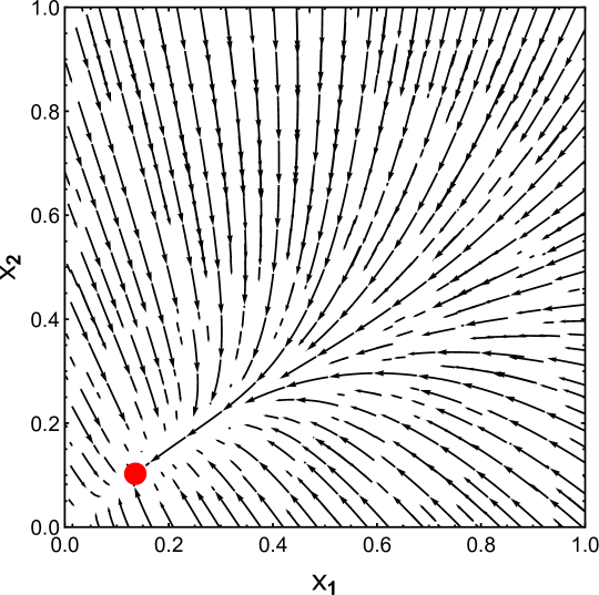
When there is no control, i.e. , the vector-valued function
| (24) |
defines the dynamics of Eq. (4), and represents the vector field shown in Fig. 2. Since , the endemic equilibrium (the red dot) is attractive for all , as per Proposition 1, Item 2, and Theorem 4.
We then introduce the feedback controllers and into the SIS network model, given in Eq. (19). The resulting vector field is shown Fig. 3, represented by the vector-valued function
| (25) |
Although the introduction of the has modified the vector-valued function to become , there remains a unique zero in . In the context of the SIS model, there is a unique endemic equilibrium , and consistent with Theorem 4, all trajectories with converge to . Comparing Fig. 2 and 3, one sees that the feedback control has shifted the endemic equilibrium from to , which clearly obeys the inequality as detailed in Lemma 5.

To summarise, Theorem 4 provides us with conclusions on a broad class of decentralised feedback controllers. Specifically, if the underlying uncontrolled system has a unique endemic equilibrium (that is convergent for all ), then no matter how we design the control functions , there will always be a unique endemic equilibrium that is convergent for all . In the language of Theorem 1, introduction of modifies the vector-valued function in Eq. (24) to become in Eq. (25), but does not change the stability of the Jacobian at any zero in , preserving the uniqueness property. This demonstrates the challenge of attempting decentralised control where each node only utilises local state for information. Nonetheless, Lemma 5 demonstrates that some health benefits are obtained, since there is a smaller fraction of infected individuals at each population.
From Theorem 3, the healthy equilibrium is globally asymptotically stable for the controlled network if and only if the underlying uncontrolled network itself has the property that is globally asymptotically stable, i.e. . If , one may wish to consider other decentralised or distributed control methods, including controlling the infection rates as functions of , e.g. . If only local information for population is available, one might require nonsmooth or time-varying or adaptive controllers; in this case the Poincaré-Hopf theorem, and consequently Theorem 1, is not applicable (at least not without significant modifications).
IV-D Discussions on the Analysis Framework
To conclude this section, we use the result of Theorem 4 to drive our discussion on the strengths and weaknesses of our analysis framework, including especially Theorem 1.
Theorem 1 establishes local exponential stability of the unique equilibrium , and notice that this does not exclude the possibility of limit cycles or chaos. Indeed, in the next section, we consider a different biological system model known to exhibit limit cycles and chaotic behaviour, and derive a sufficient condition for a unique equilibrium without requiring global convergence to . However, if one believes there is global convergence, then proving the uniqueness of can be a critical step, as it may inform of potential approaches for studying convergence. In existing work, a sufficient condition is identified using monotone systems theory that guarantees Eq. (1) for all initial conditions either converges to , or converges to a unique equilibrium in [35, Theorem 11]. However, such a result does not help to establish whether actually exists. Moreover, [35, Theorem 11] cannot be used to obtain Theorem 4, since the required condition is satisfied for the uncontrolled SIS system Eq. (4), but is not guaranteed to be satisfied for the controlled SIS system Eq. (19).
One advantage of Theorem 1 is that it enables one to analyse modifications to existing models, without significantly changing the analysis technique. In Section IV-B, we modified the standard SIS network model by adding decentralised feedback control, in the process destroying the quadratic character of the differential equation set. Application of Theorem 1 to cover a broad class of controllers involves only minor adjustments between the analysis of the uncontrolled network (Theorem 2) and the controlled network (Theorem 4). The same technique as in Theorem 4 can also be used to analyse another variant of the SIS model, known as the SIS network model in a “patchy environment” [43, 44], which aims to capture infection due to individuals travelling between population nodes.
In contrast, the algebraic-based approach of [17, 18, 16] has the advantage of being able to explicitly compute (albeit in a centralised way) the endemic equilibrium for Eq. (4), and examine weakly connected networks [17] or nodes with zero recovery rates, [22]. However, such an approach cannot be easily adapted to the patchy environment SIS model or handle broad classes of feedback control as in Section IV-B. The Lyapunov-based approach of [1] can be used to study the patchy environment models [45], and has the advantage of simultaneously establishing the uniqueness of the endemic equilibrium and global convergence. However, the Lyapunov functions of [1, 45] cannot be extended to consider the model with decentralised feedback control, as we did in Section IV-B. One requires searching for a new Lyapunov function, which may be difficult to identify and also may not cover a broad class of controllers as we have.
One drawback of Theorem 1 is the need to identify a manifold which has specific properties, such as being contractible and with pointing inward to at every point on the boundary . This is not always straightforward. Nonetheless, many models in the natural sciences will be well-defined for some positively invariant set of the state space, which may be used as a basis to inform the identification of . Once has been identified, it may be reused for modified variants of the system. In Section IV-A, we identify an appropriate for the uncontrolled SIS network model given in Eq. (4); a near identical can be used for the controlled SIS network model given in Eq. (19).
V Lotka–Volterra Systems
We now illustrate the versatility of Theorem 1 (from Section III), by applying it to a different model in the natural sciences. While Section IV considers the SIS networked epidemic model, including with feedback control, this section considers the generalised nonlinear Lotka–Volterra model. We use Theorem 1 to identify conditions for the existence of a unique non-trivial equilibrium, and establish its local stability property. We require some additional linear algebra results. For a matrix , whose diagonal entries satisfy , consider the following four conditions:
-
C1
There exists a positive diagonal such that is strictly diagonally dominant, i.e. there holds
(26) -
C2
There exists a diagonal positive for which is positive definite.
-
C3
All the leading principal minors of are positive.
-
C4
is a nonsingular -matrix (see Lemma 2).
Two simple lemmas flow from this.
Lemma 6 ([28, Chapter 6]).
Lemma 7.
The proof is straightforward, and follows by observing that each of the inequalities in Eq. (26) holds with and replaced by and respectively, in view of the inequalities in the lemma statement.
V-A Generalised Nonlinear Lotka–Volterra Models
The basic Lotka–Volterra models consider a population of biological species, with the variable associated to species . Typically, denotes the population size of species and has dynamics
| (27) |
With , the matrix form is given by
| (28) |
where and . For the matrix , there are no a priori restrictions on the signs of the , though generally diagonal terms are taken as negative. It is understood that almost exclusively, interest is restricted to systems in Eq. (28) with and such that implies for all . That is, the positive orthant is a positive invariant set of Eq. (28).
The literature on Lotka-Volterra systems is vast. We note a small number of key aspects. For an introduction, one can consult [3]. Many behaviours can be exhibited; indeed, [4] establishes that an -dimensional Lotka-Volterra system can be constructed with the property that trajectories converge to an -dimensional linear subspace in which the motion can follow that of any -dimensional system. Since a second-order system can exhibit limit cycles and a third-order system can exhibit limit cycles, strange attractors or chaos, these behaviours can be found in third or fourth (or higher) order Lotka-Volterra systems. The original prey-predator system associated with the names Lotka and Volterra is second order, and can display nonattracting limit cycles, as well as having a saddle point equilibrium and a nonhyperbolic equilibrium, see [46].
The original prey-predator system assumes that and have different signs. Many higher-dimensional Lotka-Volterra systems have mixed signs for the in fact, due to the applications relevance. Nevertheless those for which all are positive (cooperative systems) and all are negative (competitive systems) have enjoyed significant attention.
A generalization of the Lotka-Volterra system in Eq. (27) is proposed in [23] as
| (29) |
for . The are assumed to be at least two times continuously differentiable, and Eq. (27) is obtained with the identification
One can write the vector form of Eq. (29) as
| (30) |
where , and we assume Eq. (30) is such that implies for all . It is obvious that Eq. (30) has the trivial equilibrium . We comment now on other equilibria in the positive orthant. A non-trivial equilibrium is termed feasible. An equilibrium is termed partially feasible if there exist such that and . We are interested in establishing a condition for the existence and uniqueness of a feasible equilibrium for Eq. (30).
If each in Eq. (29) has the property that it is positive everywhere on the boundary of the positive orthant where , there can be no stable equilibria on the boundary, and just inside such a boundary, motions will have a component along the inwardly directed normal to the boundary. If the have the further property that whenever is such that for some constant , there holds , then the motions of Eq. (30) will be pointed inwards into when . Note that such an assumption on ensures that the population size of species does not tend to infinity for any , ensuring the population dynamics are well-defined for all time. By using Proposition 2 it follows that the interior of the set is an invariant of the motion. We now use Theorem 1 to derive a sufficient condition for Eq. (30) to have a unique feasible equilibrium.
Theorem 5.
Consider the system Eq. (30) with for all . Suppose that there exist constants such that is a positive invariant set and points inward at every . Then, there exists a feasible equilibrium in . Suppose further that for any equilibrium point :
| (31) | |||||
for some constant matrix for which satisfies C3. Then, there is a unique feasible equilibrium , and is locally exponentially stable.
Proof.
Now because of the assumption on the , an argument set out in [15, Lemma 4.1] and appealing to Brouwer’s Fixed Point Theorem establishes that there is at least one equilibrium point in the convex and compact set . Notice that all equilibria are feasible, satisfying . It follows from Eq. (30) that .
Let denote the Jacobian of the vector-valued function evaluated at . The Jacobian of the system Eq. (30), denoted to be consistent with the notation in Section III, is computed to be
which at an equilibrium is simply
| (32) |
First observe that the inequalities in Eq. (31) imply that for and this means that has all off-diagonal entries nonpositive. Lemma 6 establishes that satisfying C3 (as per the theorem hypothesis) is equivalent to being a nonsingular -matrix, and this is in turn equivalent to the existence of a positive diagonal for which is strictly diagonally dominant. Using Lemma 7 and Eq. (31), it is then evident that is strictly diagonally dominant, and it follows that is also strictly diagonally dominant. That is, satisfies C1. Lemma 6 implies that there exists a diagonal positive for which
is positive definite (Condition C2). Since is a positive definite matrix, this implies has all eigenvalues in the left half plane. The inequality Eq. (31) is assumed to hold for all equilibria , which implies that is Hurwitz for all equilibria . Theorem 1 then establishes that there is in fact a unique feasible equilibrium , and is locally exponentially stable. ∎
If in fact Eq. (31) holds for all , then one has global convergence: for all exponentially fast. To establish this, first recall that for each . Observe that for each one has
| (33) |
with taking some value existing by the mean value theorem between and . Now set for each . It is not hard to verify using Eq. (31) and Eq. (33) that
| (34) |
where is defined in Theorem 5. Let and . Consider the system
From Eq. (34), we obtain that for all . The properties of detailed in Theorem 5 allows the main theorem of [47] to be applied, which establishes that for all . Because is Hurwitz, it follows that , and therefore converges to zero, as required.
Remark 4.
It was first established in [23] that if Eq. (31) holds for all , then for all , where is a feasible equilibrium. The uniqueness of was never explicitly proved in [23], but rather implicitly by constructing a complex Lyapunov-like function which simultaneously yielded uniqueness and convergence. Theorem 5 relaxes the result of [23] in the sense that the inequalities in Eq. (31) are only required to hold when for all and , and we explicitly prove the uniqueness property. Moreover, it is conceivable that some forms of Eq. (30) have a unique feasible equilibrium while still exhibiting chaotic behaviour, limit cycles and other dynamical behaviour associated with Lotka–Volterra systems. We then, separately, recover the global convergence result of [23] by a simple argument without requiring Lyapunov-like functions.
VI A Discrete-Time Counterpart
For many processes in the natural and social sciences, both continuous- and discrete-time models exist. For example, various works have studied discrete-time epidemic models [48, 49] and Lotka–Volterra models [50]. As a consequence, it is natural for systems and control engineers to consider the same set of questions for both continuous- and discrete-time models, such as the uniqueness of the equilibrium. (Whether continuous- or discrete-time models are more appropriate is beyond the scope of this paper, and often depends on the problem context and other factors). In this section, we present a discrete-time counterpart to Theorem 1 for the nonlinear system
| (35) |
and show an example application on the DeGroot–Friedkin model of a social network [26, 51]. This counterpart result first appeared in [24, Theorem 3]. Note that a point satisfying is said to be a fixed point of the nonlinear mapping , and is an equilibrium of Eq. (35).
Theorem 6.
Consider a smooth map where is a compact and contractible manifold of finite dimension. Suppose that for all fixed points of , the eigenvalues666As defined in Section III-A, is the Jacobian of in the local coordinates of . of have magnitude less than 1. Then, has a unique fixed point , and in a local neighbourhood about , Eq. (35) converges to exponentially fast.
Rather than present the proof of the theorem, which can be found in [24] and requires some additional knowledge and results on the Lefschetz–Hopf Theorem [25, 52], we instead provide some comments relating Theorems 1 and 6. First, we note that the existence of a homotopy between and the identity map is central to the proof of Theorem 6, as detailed in [24, Theorem 3]. Consequently, [24] required to be a compact, oriented and convex manifold or a convex triangulable space of finite dimension so that a specific homotopy between and the identity map could be constructed. However, [52, Theorem 5.19] identifies that for any compact and contractible , there exists a homotopy between any map and the identity map. Thus, we can relax the hypothesis in Theorem 6 from [24, Theorem 3] to allow for to be compact and contractible.
Mutatis mutandis, Theorems 1 and 6 are therefore equivalent. The requirement in Theorem 1 that is Hurwitz for all zeroes of in Eq. (1) is equivalent to the requirement in Theorem 6 that for all fixed points of in Eq. (35), has eigenvalues all with magnitude less than 1.
Application to the DeGroot–Friedkin Model
In [24], Theorem 6 is applied to the DeGroot–Friedkin model [26], which describes the evolution of individual self-confidence, , as a social network of individuals discusses a sequence of issues, . We provide a summary of the application here. The map in question is:
| (36) |
where , and . The compact, convex and oriented manifold of interest is
where is arbitrarily small. One can regard as a compact subset in the interior of the -dimensional unit simplex, and it can be shown that for sufficiently small [26, 51].
Now, the in Eq. (36) is given with coordinates in , whereas is a manifold of dimension . Thus, an appropriate coordinate basis is proposed in [24], with an associated map on the manifold . Then, [24] establishes that the eigenvalues of at every fixed point are all of magnitude less than 1. This is done by showing that the eigenvalues of are a subset of the eigenvalues of a Laplacian matrix associated with a strongly connected graph. It is well known that such a Laplacian has a single zero eigenvalue and all other eigenvalues have positive real part. In fact, [24] shows the particular has all real eigenvalues, and its trace is 1. Since , it immediately follows that all eigenvalues of , and by implication all eigenvalues of are less than 1 in magnitude.
One can then apply Theorem 6 to establish that has a unique fixed point in (and consequently the in Eq. (36)), and is locally exponentially stable for the system Eq. (35). We refer the reader to [24, Theorem 4] for the details. We conclude by remarking that the first proof of the uniqueness of in for in Eq. (36) required extensive and complex algebraic manipulations, see [26, Appendix F]. In comparison, the calculations required to establish the uniqueness of in for in Eq. (36) using Theorem 6 are greatly simplified, and may continue to hold for generalisations of Eq. (36) as studied in [53].
VII Conclusions
We have used the Poincaré–Hopf Theorem to prove that a nonlinear dynamical system has a unique equilibrium (that is actually locally exponentially stable) if inside a compact and contractible manifold, its Jacobian at every possible equilibrium is Hurwitz. We illustrated the method by applying it to analyse the established deterministic SIS networked model, and an extension that introduces decentralised controllers, rendering the system no longer quadratic. We proved a general impossibility result: if the uncontrolled system has a unique endemic equilibrium, then the controlled system also has a unique endemic equilibrium, which is locally exponentially stable. I.e., the controllers can never globally drive the networked system to the healthy equilibrium. A stronger, almost global convergence result was obtained by extending a result from monotone dynamical systems theory, with the extension relying on the fact that the endemic equilibrium was unique. A generalised nonlinear Lotka–Volterra model was also analysed. Last, a counterpart sufficient condition was presented for a nonlinear discrete-time system to have a unique equilibrium in a compact and contractible manifold. For future work, we hope expand the analysis framework presented in this paper, and identify further applications, especially focusing on various models within the natural sciences. This includes the introduction of control to other existing epidemic models.
Appendix A Monotone Systems
A simple introduction to monotone systems is provided, sufficient for the purposes of this paper. A general convergence result is then developed, to be used in Section IV-B. For details, the reader is referred to [21, 20]. We impose slightly more restrictive conditions than in [21, 20] for the purposes of maintaining the clarity and simplicity of this section.
To begin, let , with for . Then, an orthant of can be defined as
| (37) |
For a given orthant , we write and if and , respectively.
We consider the system Eq. (1) on a convex, open set , and assume that is sufficiently smooth such that exists for all , and the solution is unique for every initial condition in . We use to denote the solution of Eq. (1) with . If whenever , satisfying , implies for all for which both and are defined, then the system Eq. (1) is said to be a type monotone system and the solution operator of Eq. (1) is said to preserve the partial ordering for . The following is a necessary and sufficient condition for Eq. (1) to be type monotone, and focuses on the Jacobian of in Eq. (1).
Lemma 8 (Kamke–Müller Condition [20, Lemma 2.1]).
Suppose that is of class in , where is open and convex in . Then, of Eq. (1) preserves the partial ordering for if and only if has all off-diagonal entries nonnegative for every , where .
Many results exist establishing convergence of type monotone systems, with various additional assumptions imposed. Here, we state one which has some stricter assumptions, and then extend it for use in our analysis in Section IV-B. Let denote the set of equilibria of Eq. (1), and for an equilibrium , the basin of attraction of is denoted by . We say Eq. (1) is an irreducible type monotone system if is irreducible for all .
Lemma 9 ([20, Theorem 2.6]).
Let be an open, bounded, and positively invariant set for an irreducible type monotone system Eq. (1). Suppose the closure of , denoted by , contains a finite number of equilibria. Then,
| (38) |
is open and dense in .
A set is dense in if every point is either in or in the closure of . Thus, Lemma 9 states that for an irreducible type monotone system Eq. (1), the system converges to an equilibrium for almost all initial conditions in . There are at most a finite number of nonattractive limit cycles. A stronger result is available, appearing in [54, Theorem D], and presented below with a different, simpler proof. The result will be used in Section IV.
Proposition 4 (c.f. [54, Theorem D]).
Let be an open, bounded, convex, and positively invariant set for an irreducible type monotone system Eq. (1). Suppose there is a unique equilibrium and no equilibrium in . Then, convergence to occurs for every initial condition in .
Proof.
First, we remark that an irreducible type monotone system Eq. (1) enjoys a stronger monotonicity property; for any , one has that for all [21].
In light of Lemma 9, the proposition is proved if we establish that there does not exist a limit cycle. We argue by contradiction. Let be a point on such a limit cycle of Eq. (1). Pick two points and satisfying , and observe that there exist two sufficiently small balls and surrounding and , respectively, which neither intersect the boundary of nor contain , and every point and obey . Since almost every point in is not in a nonattractive limit cycle, there exists an such that . Similarly, there exists a such that . Because , it follows that . Recalling that and yields . However, this contradicts the assumption that is a point on a nonattractive limit cycle. ∎
Appendix B Proof of Lemma 4
To begin, we prove the first part of the lemma statement. Fixing , we need to show that for . Now, satisfies and for , we have for some . From Eq. (3), we find
| (39) |
The identity implies , and substituting this into the above and rearranging yields
| (40) |
Since is constant and for all , there exists a sufficiently small such that for all , the first and second summand on the right of Eq. (40) are positive and nonnegative, respectively. It follows from Eq. (40) that for all . Repeating the analysis for , it is clear that Eq. (15a) holds for all , for any positive .
Next, fix , and consider a point . Now, , and Eq. (3) yields , and this holds for all , and thus Eq. (15b) holds. It follows from Proposition 2 that for , is a positive invariant set of Eq. (4). Eq. (15) shows that is not an invariant set of Eq. (4), which implies that is also a positive invariant set of Eq. (4).
To prove the second part of the lemma, consider a point , at some time . If for some , then Eq. (3) yields . Thus, if , then obviously for some sufficiently small positive and .
Let us suppose then, that has at least one zero entry. Define the set . The lemma hypothesises that is strongly connected, which implies that there exists a such that for some . Eq. (3) yields . This analysis can be repeated to show that there exists a finite such that is empty. It follows that for some sufficiently small .
Since is bounded, there exists a finite and sufficiently small such that for all . Since can be taken to be arbitrarily small, it is also clear that any nonzero equilibrium must satisfy . ∎
Appendix C Proof of Lemma 5
Let denote the endemic equilibrium of Eq. (19), and . Note the assumption that there exists a such that implies is not only a nonnegative diagonal matrix, but has at least one positive entry. Observe that Eq. (19) and
| (41) |
have the same positive equilibrium . By arguments introduced previously, we know that is the only positive equilibrium for Eq. (41). Hence by Proposition 1. Let be a sufficiently large constant such that is nonnegative for all (note that is irreducible). The Perron–Frobenius Theorem [28] yields . For , one concludes that is equal to plus some nonnegative diagonal entries (of which at least one is positive), and [28, Corollary 2.1.5] yields that . This implies that . It follows that for all . Hence the system
| (42) |
has for all a unique equilibrium in , call it . Notice that (the endemic equilibrium of the uncontrolled system Eq. (4)) and .
Since is diagonal, there holds , where . Then, differentiating
with respect to yields after some rearranging:
| (43) |
Using arguments similar to those laid out in the proof of Theorem 2 (see Eq. 16 and below) it can be shown that is an irreducible, nonsingular -matrix. [28, Theorem 2.7] yields that . Next, one can verify that has at least one positive entry since has at least one positive entry and . This means that
Integration yields , as claimed. ∎
Appendix D Properties of the Tangent Cone
We now prove the claims below Eq. (6), that identify the relationship between and , for a smooth and compact -dimensional manifold embedded in , with .
To begin, we state the following well known result, which can be established from the material in [32, pg. 8–10].
Proposition 5.
The tangent space at a point in a -dimensional manifold embedded in is an -dimensional Euclidean space (“hyperplane” in the case of ) in .
The following lemma, which is intuitively obvious, is also required.
Lemma 10.
Let be two points outside a compact set . Then there holds
Proof.
Consider two paths and the associated distances from to . The first is that via the shortest distance path, which is , and the second is that via the shortest path which is constrained to pass through . The second is never shorter than the first, which is the content of the inequality. ∎
D-A Manifolds Without Boundary
In this subsection, we shall assume that the manifold does not have a boundary. We shall treat the case of manifolds with a boundary in the next subsection. The tangent cone of at is defined in Eq. (6). We shall distinguish and , treating these in order. The first result is asserted in [30] for , but that reference does not consider .
Proposition 6.
With notation as above, suppose . Then .
Proof.
Observe first that by the compactness of , is attained at some . Moreover is necessarily nonzero, assuming a value say, since otherwise we would have , a contradiction. Now use Lemma 10, identifying and with and respectively. We have
It follows that for no , can we have
This completes the proof. ∎
We now turn our focus onto the case . Our aim is to show that for all , thus linking the concepts of a tangent cone and a tangent space. We first of all establish a one-way inclusion.
Proposition 7.
With notation as above and , there holds .
Proof.
Suppose but is otherwise arbitrary. Let the smooth function be a local parametrisation around with . Then there exists a such that . (In a particular coordinate basis, is simply equal to , where is the Jacobian matrix of evaluated at , and is a vector.) Observe then that
Then for sufficiently small,
by the “best linear approximation” interpretation of , c.f. [32, pg. 9]. This means that
Observe that lies in . So the distance from to is overbounded by This distance divided by is therefore overbounded by . Hence as goes to zero, this bound goes to zero. This implies that is in by Eq. (6). But was an arbitrary vector in . This establishes that is contained in . ∎
It remains to prove the reverse inclusion. In the case of , the tangent space corresponds to the whole space in which is embedded, and so , which establishes the claim that the tangent cone and the tangent space coincide. Thus, we now need to focus just on the case .
Proposition 8.
With notation as above, and , there holds
Proof.
Suppose, in order to obtain a contradiction, that , while also . Set , where and is orthogonal to . Suppose that is attained at for some , depending on and . Such a exists if is sufficiently small. Now, observe that
Note that the second equality was obtained by using the ‘best linear approximation’, c.f. [32, pg. 9]. Now, since , it follows that, irrespective of the particular and thus the particular , there holds
Thus,
From this, it follows that because , which is a contradiction. ∎
D-B Manifolds With Boundary
We now assume that , in addition to the properties detailed and the start of Appendix D, also has a boundary , and that boundary is also smooth. It is necessary at the outset to modify the definition of the tangent cone in Eq. (6) to distinguish directions associated with any value of on , so that it is defined using one-sided limits:
| (44) |
For manifolds without a boundary, the two definitions are evidently equivalent.
It is straightforward to see that key results of the previous subsection remain valid, with essentially unchanged proofs. In fact:
-
1.
Proposition 6 remains valid;
- 2.
The remaining interest is in the case when . In the case where and assuming the boundary is smooth at , the tangent cone is just the tangent half-space but shifted to the origin, as observed explicitly in the reference [30]. This reference does not actually prove the result, but it is easily obtained using the methods of the previous section, using the adjusted notion of the tangent cone in Eq. (44). And indeed, this continues to hold for the case , rather than just .
References
- [1] Z. Shuai and P. van den Driessche, “Global stability of infectious disease models using lyapunov functions,” SIAM Journal on Applied Mathematics, vol. 73, no. 4, pp. 1513–1532, 2013.
- [2] M. Y. Li and Z. Shuai, “Global-stability problem for coupled systems of differential equations on networks,” Journal of Differential Equations, vol. 248, no. 1, pp. 1–20, 2010.
- [3] Y. Takeuchi, Global Dynamical Properties of Lotka–Volterra Systems. World Scientific, 1996.
- [4] S. Smale, “On the Differential Equations of Species in Competition,” Journal of Mathematical Biology, vol. 3, no. 1, pp. 5–7, 1976.
- [5] J. W. Milnor, Topology from the Differentiable Viewpoint. Princeton University Press, 1997.
- [6] M. A. Belabbas, “On Global Stability of Planar Formations,” IEEE Transactions on Automatic Control, vol. 58, no. 8, pp. 2148–2153, Aug 2013.
- [7] S. M. Moghadas, “Analysis of an epidemic model with bistable equilibria using the poincaré index,” Applied Mathematics and Computation, vol. 149, no. 3, pp. 689–702, 2004.
- [8] A. Simsek, A. Ozdaglar, and D. Acemoglu, “Generalized Poincare-Hopf Theorem for compact Nonsmooth Regions,” Mathematics of Operations Research, vol. 32, no. 1, pp. 193–214, 2007.
- [9] A. Tang, J. Wang, S. H. Low, and M. Chiang, “Equilibrium of Heterogeneous Congestion Control: Existence and Uniqueness,” IEEE/ACM Transactions on Networking, vol. 15, no. 4, pp. 824–837, Aug 2007.
- [10] F. Christensen, “A necessary and sufficient condition for a unique maximum with an application to potential games,” Economics Letters, vol. 161, pp. 120–123, 2017.
- [11] S. Henshaw and C. C. McCluskey, “Global stability of a vaccination model with immigration,” Electronic Journal of Dierential Equations, vol. 92, pp. 1–10, 2015.
- [12] A. Konovalov and Z. Sándor, “On price equilibrium with multi-product firms,” Economic Theory, vol. 44, no. 2, pp. 271–292, 2010.
- [13] F. J. A. Rijk and A. C. F. Vorst, “Equilibrium points in an urban retail model and their connection with dynamical systems,” Regional Science and Urban Economics, vol. 13, no. 3, pp. 383–399, 1983.
- [14] H. R. Varian, “A third remark on the number of equilibria of an economy,” Econometrica, vol. 43, no. 5-6, p. 985, 1975.
- [15] A. Lajmanovich and J. A. Yorke, “A Deterministic Model for Gonorrhea in a Nonhomogeneous Population,” Mathematical Biosciences, vol. 28, no. 3-4, pp. 221–236, 1976.
- [16] A. Fall, A. Iggidr, G. Sallet, and J.-J. Tewa, “Epidemiological Models and Lyapunov Functions,” Mathematical Modelling of Natural Phenomena, vol. 2, no. 1, pp. 62–83, 2007.
- [17] A. Khanafer, T. Başar, and B. Gharesifard, “Stability of epidemic models over directed graphs: A positive systems approach,” Automatica, vol. 74, pp. 126–134, 2016.
- [18] W. Mei, S. Mohagheghi, S. Zampieri, and F. Bullo, “On the dynamics of deterministic epidemic propagation over networks,” Annual Reviews in Control, vol. 44, pp. 116–128, 2017.
- [19] P. V. Mieghem, J. Omic, and R. Kooij, “Virus spread in networks,” IEEE/ACM Transactions on Networking, vol. 17, no. 1, pp. 1–14, 2009.
- [20] H. L. Smith, “Systems of Ordinary Differential Equations Which Generate an Order Preserving Flow. A Survey of Results,” SIAM Review, vol. 30, no. 1, pp. 87–113, 1988.
- [21] ——, Monotone Dynamical Systems: An Introduction to the Theory of Competitive and Cooperative Systems. American Mathematical Society: Providence, Rhode Island, 2008, vol. 41.
- [22] J. Liu, P. E. Paré, A. Nedich, C. Y. Tang, C. L. Beck, and T. Başar, “Analysis and Control of a Continuous-Time Bi-Virus Model,” IEEE Transactions on Automatic Control, vol. 64, no. 12, pp. 4891–4906, Dec. 2019.
- [23] B. S. Goh, “Sector stability of a complex ecosystem model,” Mathematical Biosciences, vol. 40, no. 1-2, pp. 157–166, 1978.
- [24] B. D. O. Anderson and M. Ye, “Nonlinear Mapping Convergence and Application to Social Networks,” in European Control Conference, Limassol, Cyprus, Jun. 2018, pp. 557–562.
- [25] M. W. Hirsch, Differential Topology. Springer Science & Business Media, 2012, vol. 33.
- [26] P. Jia, A. MirTabatabaei, N. E. Friedkin, and F. Bullo, “Opinion Dynamics and the Evolution of Social Power in Influence Networks,” SIAM Review, vol. 57, no. 3, pp. 367–397, 2015.
- [27] M. Ye, J. Liu, B. D. O. Anderson, and M. Cao, “Distributed Feedback Control on the SIS Network Model: An Impossibility Result,” in 21st IFAC World Congress, Berlin, 2020.
- [28] A. Berman and R. J. Plemmons, Nonnegative Matrices in the Mathematical Sciences, ser. Computer Science and Applied Mathematics. Academic Press: London, 1979.
- [29] C. Nowzari, V. M. Preciado, and G. J. Pappas, “Analysis and Control of Epidemics: A Survey of Spreading Processes on Complex Networks,” IEEE Control Systems, vol. 36, no. 1, pp. 26–46, 2016.
- [30] F. Blanchini, “Set invariance in control,” Automatica, vol. 35, no. 11, pp. 1747–1767, 1999.
- [31] M. Ye, J. Liu, B. D. O. Anderson, and M. Cao, “Applications of the Poincaré–Hopf Theorem: Epidemic Models and Lotka–Volterra Systems,” provisionally accepted in IEEE Transactions on Automatic Control, 2020. [Online]. Available: https://arxiv.org/abs/1911.12985
- [32] V. Guillemin and A. Pollack, Differential Topology. American Mathematical Soc., 2010, vol. 370.
- [33] S. Sastry, Nonlinear systems: analysis, stability, and control. Springer New York, 1999, vol. 10.
- [34] M. A. Khamsi and W. A. Kirk, An Introduction to Metric Spaces and Fixed Point Theory. John Wiley & Sons, 2011.
- [35] J. A. Jacquez and C. P. Simon, “Qualitative Theory of Compartmental Systems,” SIAM Review, vol. 35, no. 1, pp. 43–79, 1993.
- [36] Z. Qu, Cooperative Control of Dynamical Systems: Applications to Autonomous Vehicles. Springer Science & Business Media, 2009.
- [37] V. M. Preciado, M. Zargham, C. Enyioha, A. Jadbabaie, and G. Pappas, “Optimal Resource Allocation for Network Protection: A Geometric Programming Approach,” IEEE Transactions on Control of Network Systems, vol. 1, no. 1, pp. 99–108, 2014.
- [38] N. J. Watkins, C. Nowzari, V. M. Preciado, and G. J. Pappas, “Optimal Resource Allocation for Competitive Spreading Processes on Bilayer Networks,” IEEE Transactions on Control of Network Systems, vol. 5, no. 1, pp. 298–307, 2018.
- [39] Y. Wan, S. Roy, and A. Saberi, “Designing spatially heterogeneous strategies for control of virus spread,” IET Systems Biology, vol. 2, no. 4, pp. 184–201, 2008.
- [40] J. A. Torres, S. Roy, and Y. Wan, “Sparse Resource Allocation for Linear Network Spread Dynamics,” IEEE Transactions on Automatic Control, vol. 62, no. 4, pp. 1714–1728, 2016.
- [41] V. S. Mai, A. Battou, and K. Mills, “Distributed Algorithm for Suppressing Epidemic Spread in Networks,” IEEE Control Systems Letters, vol. 2, no. 3, pp. 555–560, 2018.
- [42] H. Hemilä, “Zinc lozenges and the common cold: a meta-analysis comparing zinc acetate and zinc gluconate, and the role of zinc dosage,” Journal of Royal Society of Medicine Open, vol. 8, no. 5, p. 2054270417694291, 2017.
- [43] W. Wang and X.-Q. Zhao, “An epidemic model in a patchy environment,” Mathematical Biosciences, vol. 190, no. 1, pp. 97–112, 2004.
- [44] Y. Jin and W. Wang, “The effect of population dispersal on the spread of a disease,” Journal of Mathematical Analysis and Applications, vol. 308, no. 1, pp. 343–364, 2005.
- [45] M. Y. Li and Z. Shuai, “Global stability of an epidemic model in a patchy environment,” Canadian Applied Mathematics Quarterly, vol. 17, no. 1, pp. 175–187, 2009.
- [46] M. Vidyasagar, Nonlinear Systems Analysis. SIAM, 2002, vol. 42.
- [47] W. Walter, “Ordinary Differential Inequalities in Ordered Banach Spaces,” Journal of Differential Equations, vol. 9, no. 2, pp. 253–261, 1971.
- [48] L. J. S. Allen, “Some Discrete-Time , , and Eepidemic Models,” Mathematical biosciences, vol. 124, no. 1, pp. 83–105, 1994.
- [49] K. Prem, Y. Liu, T. W. Russell, A. J. Kucharski, R. M. Eggo, N. Davies, S. Flasche, S. Clifford, C. A. Pearson, J. D. Munday et al., “The effect of control strategies to reduce social mixing on outcomes of the COVID-19 epidemic in Wuhan, China: a modelling study,” The Lancet Public Health, vol. 5, no. 5, pp. 261–270, May 2020.
- [50] Q. Din, “Dynamics of a discrete Lotka-Volterra model,” Advances in Difference Equations, vol. 2013, no. 1, p. 95, 2013.
- [51] M. Ye, J. Liu, B. D. O. Anderson, C. Yu, and T. Başar, “Evolution of Social Power in Social Networks with Dynamic Topology,” IEEE Transaction on Automatic Control, vol. 63, no. 11, pp. 3793–3808, Nov. 2018.
- [52] M. A. Armstrong, Basic Topology. Springer Science & Business Media, 2013.
- [53] M. Ye and B. D. O. Anderson, “Modelling of Individual Behaviour in the DeGroot–Friedkin Self-Appraisal Dynamics on Social Networks,” in European Control Conference, Naples, Italy, Jun. 2019, pp. 2011–2017.
- [54] J. Ji-Fa, “On the global stability of cooperative systems,” Bulletin of the London Mathematical Society, vol. 26, no. 5, pp. 455–458, 1994.
![[Uncaptioned image]](/html/1911.12985/assets/Figures/profile_pic_RUG.jpg) |
Mengbin Ye (S’13-M’18) was born in Guangzhou, China. He received the B.E. degree (with First Class Honours) in mechanical engineering from the University of Auckland, Auckland, New Zealand in 2013, and the Ph.D. degree in engineering at the Australian National University, Canberra, Australia in 2018. From 2018-2020, he was a postdoctoral researcher with the Faculty of Science and Engineering, University of Groningen, Netherlands. Since 2020, he is an Optus Fellow at the Optus–Curtin Centre of Excellence in Artificial Intelligence, Curtin University, Perth, Australia. He has been awarded the 2018 J.G. Crawford Prize (Interdisciplinary), ANU’s premier award recognising graduate research excellence. He has also received the 2018 Springer PhD Thesis Prize, and was Highly Commended in the Best Student Paper Award at the 2016 Australian Control Conference. His current research interests include opinion dynamics and decision making in complex social networks, epidemic modelling, coordination of multi-agent systems, and localisation using bearing measurements. |
![[Uncaptioned image]](/html/1911.12985/assets/Figures/photo_liu.jpg) |
Ji Liu (S’09-M’13) received the B.S. degree in information engineering from Shanghai Jiao Tong University, Shanghai, China, in 2006, and the Ph.D. degree in electrical engineering from Yale University, New Haven, CT, USA, in 2013. He is currently an Assistant Professor in the Department of Electrical and Computer Engineering at Stony Brook University, Stony Brook, NY, USA. Prior to joining Stony Brook University, he was a Postdoctoral Research Associate at the Coordinated Science Laboratory, University of Illinois at Urbana-Champaign, Urbana, IL, USA, and the School of Electrical, Computer and Energy Engineering, Arizona State University, Tempe, AZ, USA. His current research interests include distributed control and computation, distributed optimization and learning, multi-agent systems, social networks, epidemic networks, and cyber-physical systems. |
![[Uncaptioned image]](/html/1911.12985/assets/Figures/BDOA.jpg) |
Brian D.O. Anderson (M’66-SM’74-F’75-LF’07) was born in Sydney, Australia. He received the B.Sc. degree in pure mathematics in 1962, and B.E. in electrical engineering in 1964, from the Sydney University, Sydney, Australia, and the Ph.D. degree in electrical engineering from Stanford University, Stanford, CA, USA, in 1966. He is an Emeritus Professor at the Australian National University, and a Distinguished Researcher in Data61-CSIRO (previously NICTA) and a Distinguished Professor at Hangzhou Dianzi University. His awards include the IEEE Control Systems Award of 1997, the 2001 IEEE James H Mulligan, Jr Education Medal, and the Bode Prize of the IEEE Control System Society in 1992, as well as several IEEE and other best paper prizes. He is a Fellow of the Australian Academy of Science, the Australian Academy of Technological Sciences and Engineering, the Royal Society, and a foreign member of the US National Academy of Engineering. He holds honorary doctorates from a number of universities, including Université Catholique de Louvain, Belgium, and ETH, Zürich. He is a past president of the International Federation of Automatic Control and the Australian Academy of Science. His current research interests are in distributed control, sensor networks and econometric modelling. |
![[Uncaptioned image]](/html/1911.12985/assets/Figures/Ming_172.jpg) |
Ming Cao is currently Professor of systems and control with the Engineering and Technology Institute (ENTEG) at the University of Groningen, the Netherlands, where he started as a tenure-track Assistant Professor in 2008. He received the Bachelor degree in 1999 and the Master degree in 2002 from Tsinghua University, Beijing, China, and the Ph.D. degree in 2007 from Yale University, New Haven, CT, USA, all in Electrical Engineering. From September 2007 to August 2008, he was a Postdoctoral Research Associate with the Department of Mechanical and Aerospace Engineering at Princeton University, Princeton, NJ, USA. He worked as a research intern during the summer of 2006 with the Mathematical Sciences Department at the IBM T. J. Watson Research Center, NY, USA. He is the 2017 and inaugural recipient of the Manfred Thoma medal from the International Federation of Automatic Control (IFAC) and the 2016 recipient of the European Control Award sponsored by the European Control Association (EUCA). He is an Associate Editor for IEEE Transactions on Automatic Control, IEEE Transactions on Circuits and Systems and Systems and Control Letters, and for the Conference Editorial Board of the IEEE Control Systems Society. He is also a member of the IFAC Technical Committee on Networked Systems. His research interests include autonomous agents and multi-agent systems, mobile sensor networks and complex networks. |