Magnetotransport of Weyl semimetals with tilted Dirac cones

Abstract

Weyl semimetals (WSM) exhibit chiral anomaly in their magnetotransport due to broken conservation laws. Here, we analyze the magnetotransport of WSM in the presence of the time-reversal symmetry-breaking tilt parameter. The analytical expression for the magnetoconductivity is derived in the small tilt limit using the semiclassical Boltzmann equation. We predict a planar Hall current which flows transverse to the electric field and in the plane containing magnetic and electric fields and scales linearly with the tilt parameter. A tilt-induced transverse conductivity is also present in the case where the electric and magnetic fields are parallel to each other, a scenario where the conventional Hall current completely vanishes.

I Introduction

A Weyl semimetal (WSM) state in topological systems with broken time-reversal and/or inversion symmetry can be understood by the availability of the low energy quasiparticles called Weyl fermions (WF) with linear in momentum dispersion near the crossing point of two non-degenerate bands in momentum space known as Weyl point (WP) 1367-2630-9-9-356 ; PhysRevB.83.205101 . Although the concept of WF was first introduced in relativistic field theory, it has never been observed in the systems of elementary particles, and has only very recently been realized in a condensed matter systems as an excitation of quasi-particles. The essential properties of WPs are: the presence of pairs of opposite chiralities connected by Fermi arcs on the surface and the zero-sum of chiralities over all the WPs in the Brillouin zone, according to the Nielsen-Ninomiya theorem 1983PhLB..130..389N . The chirality $\chi$ of a WP is defined by the integration of Berry curvature $\mathbf{\Omega}_{\mathbf{k}}$ ($\mathbf{\Omega}_{\mathbf{k}}=\nabla\times\mathbf{A}_{\mathbf{k}}$ with $\mathbf{A}_{\mathbf{k}}=i\left\langle u_{\mathbf{k}}|\nabla_{\mathbf{k}}u_{\mathbf{k}}\right\rangle$, where $\left|u_{\mathbf{k}}\right\rangle$ is the Bloch wave function) over a closed surface around that WP in momentum space ($\varointclockwise\text{d}\mathbf{s}\cdot\mathbf{\Omega}_{\mathbf{k}}=2\pi\chi$ where, $\chi=\pm 1,\pm 2,.....$ ).

In the presence of external electric and magnetic fields the conservation of the number of WFs with particular chirality is broken, a phenomenon known as chiral anomaly. The WSMs are distinctive from other metals/semi-metals because the chiral anomaly can lead to unusual magneto-transport phenomena. For example; the observation of negative magneto-conductivity has been attributed to the phenomenon of chiral anomaly Arnold2016 ; Li2015 ; Li2016 ; PhysRevX.5.031023 ; Xiong413 ; Zhang2016 .

In this manuscript, we study the electron transport in WSM where the Dirac cones are tilted in momentum space. Such a tilted WSM can be described by an additional anisotropy term in the Hamiltonian for electrons near the WPs as follows PhysRevB.78.045415 ,

$$H=v_{F}\bm{\sigma}\cdot\mathbf{k}+I\mathbf{w}\cdot\mathbf{k},$$ (1)

where the components of $\bm{\sigma}$ are the Pauli matrices and $I$ is the $2\times 2$ identity matrix, $\mathbf{k}$ is the wave vector, the vector $\mathbf{w}$ represents the dispersion tilt and $v_{F}$ is the Fermi velocity. The tilt $\mathbf{w}$ in Eq. (1) breaks the time-reversal symmetry (TRS). The energy eigenvalues are given by $\epsilon_{k}=(\hbar\mathbf{w}\cdot\mathbf{k}+\hbar v_{F}\mathrm{k}$) and the corresponding group velocity is $\mathbf{v_{k}}=(\mathbf{w}+v_{F}\hat{\mathrm{k}})$ (where $\hat{\mathrm{k}}$ is the unit vector along $\mathbf{k}$ and $v_{F}$ the Fermi velocity). If the value of tilt $|\mathbf{w}|<v_{F}$ then the WSMs are sub-grouped as Type-I WSM and when $|\mathbf{w}|>v_{F}$ then the WSMs are sub-grouped as Type-II WSM. A non-tilted and tilted dispersion relation in WSM is shown in the schematic diagram in Fig. 1(a). Type-II WSM phase has been observed in a range of materials such as MoTe₂, WTe₂, LaAlGe Soluyanov2015 ; Xue1603266 ; Deng2016 ; Li2017 and already several transport phenomena have been addressed in several studies PhysRevB.95.075133 ; PhysRevLett.117.077202 ; APhysRevB.94.081408 ; Zyuzin2016 .

Transport studies of tilted Weyl semimetals have been done recently such as anomalous Nernst effect PhysRevB.96.115202 ; Saha2018 , optical response to circularly polarized light PhysRevB.96.085114 and planar Halle effect (PHE) PhysRevB.99.115121 . Using Boltzmann transport it has been predicted that both the chiral anomaly and non-trivial Berry curvature effects leads to the PHE in Weyl semimetals PhysRevLett.119.176804 and very recently, PHE in half Heusler Weyl semimetal GdPtBi has been attributed to a strong Berry curvature effect PhysRevB.98.041103 .

Motivated by the above works, we analyze the role of the dispersion tilt in Berry curvature induced transport in the WSM systems, which has not been investigated hitherto. Our study reveals unusual transport properties, such as the planar Hall effect induced by the time-reversal symmetry breaking tilt and Berry curvature effects. We mainly consider tilted Type-I WSM and evaluate transport properties in response to external electric and magnetic fields. Both the longitudinal and transverse conductivities are calculated using the Boltzmann transport equation. Our manuscript is arranged as follows: in Sec. II we present the general framework of the semiclassical Boltzmann model to calculate the current density up to the second orders in the $B$ field. in Sec. III we present the analytical expression for the conductivity in the small-tilt regime. We also perform numerical calculations for arbitrary tilt value in the case of both Type-I and Type-II WSM (results of the latter are presented in more detail in the Supplemental) and verify the analytical results in the limit of small tilt. The anisotropy of the WSM conductivity with respect to the magnetic field and tilt directions is also presented. We conclude in Sec. IV.

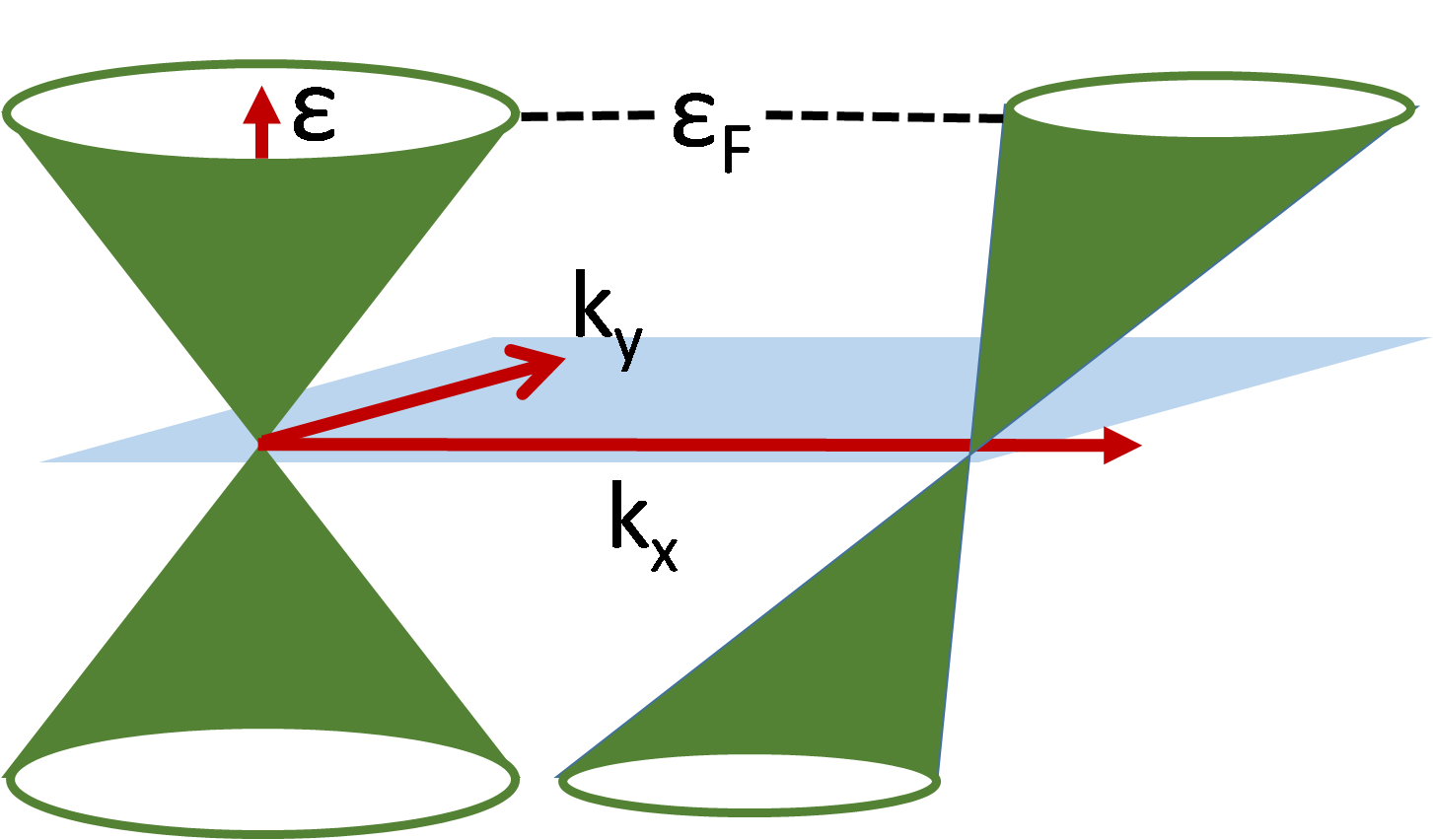
(a)

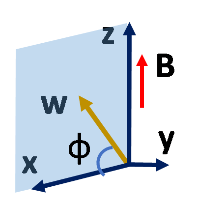
(b)

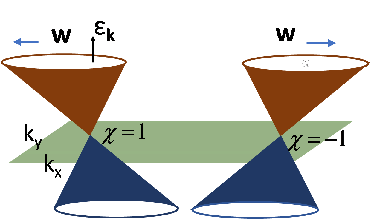
(c)

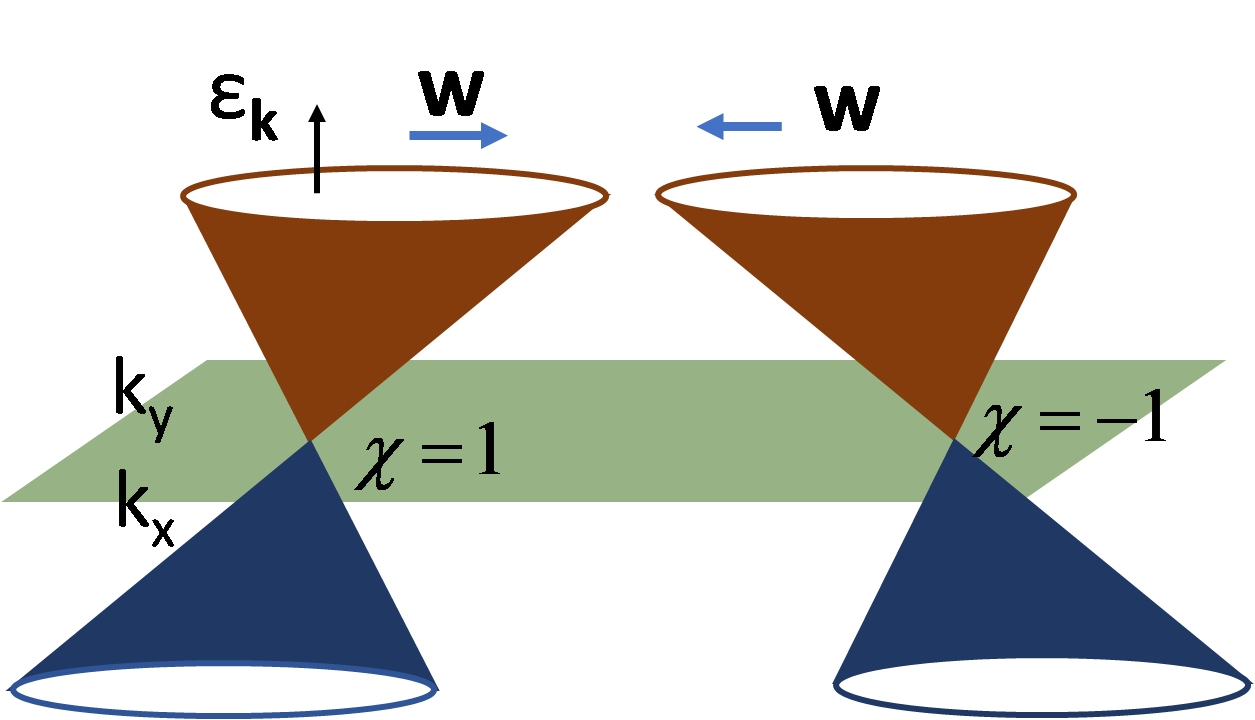
(d)

Figure 1: (Color online) (a) Dispersion relation for the non-tilted (left) and tilted (right) WSM. (b) The $z$-axis is parallel to the magnetic field while the tilt vector $\mathbf{w}$ lies on the $x$-$z$ plane with an angle $\phi$ from the $x$-axis. (c)-(d), A pair of Dirac cones are tilted (c) towards each other, and (d) away from each other.

II Method

We apply the semiclassical Boltzmann transport model under the assumption of a small external magnetic and electric fields where the separation between Landau levels can be neglected and where it is valid to use the semiclassical approach PhysRevB.88.104412 . We begin with the standard procedure to calculate the Boltzmann’s distribution function for a system with non-zero Berry curvature under the application of external electric and magnetic field. The presence of Berry curvature $\mathbf{\Omega_{k}}$ in the WSMs provides a correction to the phase space volume in the case of adiabatic transport, as shown in PhysRevB.59.14915 ; RevModPhys.82.1959 . In the presence of electric ($\mathbf{E}$) and magnetic field ($\mathbf{B}$) the semiclassical equations of motion are modified as follows PhysRevB.59.14915 ,

$$\dot{\mathbf{r}} =\left(1+\frac{e}{\hbar}\mathbf{\Omega}_{\mathbf{k}}\cdot\mathbf{B}\right)^{-1}\left[\mathbf{v_{k}}+e\mathbf{E}\times\mathbf{\Omega}_{\mathbf{k}}+\frac{e}{\hbar}(\mathbf{\Omega}_{\mathbf{k}}\cdot\mathbf{v}_{\mathbf{k}})\mathbf{B}\right],$$

$$\hbar\dot{\mathbf{k}} =\left(1+\frac{e}{\hbar}\mathbf{\Omega}_{\mathbf{k}}\cdot\mathbf{B}\right)^{-1}\left[e\mathbf{E}+\frac{e}{\hbar}\mathbf{v_{k}}\times\mathbf{B}+\frac{e^{2}}{\hbar}(\mathbf{E}\cdot\mathbf{B})\mathbf{\Omega}_{\mathbf{k}}\right],$$ (2)

where $\mathbf{v_{k}}=\partial\epsilon_{\mathbf{k}}/\hbar\partial\mathbf{k}$ is the group velocity of the electrons with $\epsilon_{\mathbf{k}}$ being the energy dispersion, $\mathbf{r}$ the position and $\hbar\mathbf{k}$ the momentum of a single electron. To evaluate the distribution $f(\mathbf{r},\mathbf{k},t)$ we consider the Boltzmann’s equation,

$$\frac{\partial f(\mathbf{r},\mathbf{k},t)}{\partial t}+\dot{\mathbf{r}}\cdot\frac{\partial f(\mathbf{r},\mathbf{k},t)}{\partial\mathbf{r}}+\dot{\mathbf{k}}\cdot\frac{\partial f(\mathbf{r},\mathbf{k},t)}{\partial\mathbf{k}}=I_{coll}\left\{f(\mathbf{r},\mathbf{k},t)\right\},$$ (3)

where $I_{coll}\left\{f(\mathbf{r},\mathbf{k},t)\right\}$ is the collision integral. We solve for the change in the distribution function $\delta f$ for a uniform system under steady-state condition, i.e., ignoring the time and space dependence in the above equation, and apply the relaxation time approximation, i.e., $I_{coll}\left\{f(\mathbf{r},\mathbf{k},t)\right\}=\delta f(\mathbf{r},\mathbf{k},t)/\tau(\mathbf{k})$. Here, $\tau(\mathbf{k})$ is the relaxation time and is assumed to be independent of $\mathbf{k}$. This is a common assumption given that more refined forms of $\tau(\mathbf{k})$ do not lead to significantly different physics PhysRevB.88.104412 . Assuming the second-order derivative of the distribution function to be negligible, the change in the distribution function is evaluated from Eqs. (2) and (3) as,

$$\delta f(\mathbf{r},\mathbf{k},t) =-\tau\left(1+\frac{e}{\hbar}\mathbf{\Omega}_{\mathbf{k}}\cdot\mathbf{B}\right)^{-1}\hbar^{-1}$$

$$\left(e\mathbf{E}+\frac{e^{2}}{\hbar}\left(\mathbf{E}\cdot\mathbf{B}\right)\mathbf{\Omega}_{\mathbf{k}}\right)\cdot\mathbf{v_{k}}\left(\partial f^{0}/\partial\epsilon\right),$$ (4)

where $\epsilon$ is the electron energy and $f^{0}$ is the equilibrium distribution function which usually can be replaced by Fermi function. As we are interested in the Berry-curvature induced effect only, we neglect the effect of Lorentz force (see the second line of Eq. (2)) which produces the conventional Hall current. The expression of current density is given by, $\mathbf{j}=\left(e/8\pi^{3}\right)\int\text{d}\mathbf{k}\text{ }(1+(e/\hbar)\mathbf{\Omega}_{\mathbf{k}}\cdot\mathbf{B})^{-1}\dot{\mathbf{r}}\delta f(\mathbf{k})$ and using the above results for a single Weyl node we obtain,

$$\mathbf{j} =\frac{e\tau}{4\pi^{3}\hbar}\int\text{d$\epsilon$}\frac{\partial f^{0}}{\partial\epsilon}\int\text{d}S\frac{1}{(1+\frac{e}{\hbar}\mathbf{\Omega}_{\mathbf{k}}\cdot\mathbf{B})|\mathbf{v_{k}}|}\left[(e\mathbf{E}\cdot\mathbf{v_{k}})\mathbf{v_{k}}\right.$$

$$+\frac{e^{2}}{\hbar}(\mathbf{E}\cdot\mathbf{B})\left((\mathbf{\Omega}_{\mathbf{k}}\cdot\mathbf{v_{k}})\mathbf{v_{k}}+\frac{e\mathbf{B}}{\hbar^{2}}(\mathbf{\Omega}_{\mathbf{k}}\cdot\mathbf{v_{k}})^{2}\right)$$

$$\left.+\frac{e^{2}\mathbf{B}}{\hbar}(\mathbf{E}\cdot\mathbf{v_{k}})(\mathbf{\Omega}_{\mathbf{k}}\cdot\mathbf{v_{k}})\right],$$ (5)

where $S$ is the area of the constant energy surface. The current density above originates due to the imbalance between the particles numbers in the right-handed and left-handed valleys in the presence of the external electric and magnetic fields (i.e., the phenomenon of chiral anomaly), as discussed in Ref. PhysRevB.88.104412 . Next, we expand $\mathbf{j}$ to various orders of magnetic field as follows: $\left(1+(e/\hbar)\mathbf{\Omega}_{\mathbf{k}}\cdot\mathbf{B}\right)^{-1}=1-(e/\hbar)\mathbf{\Omega}_{\mathbf{k}}\cdot\mathbf{B}+(e/\hbar)^{2}\left(\mathbf{\Omega}_{\mathbf{k}}\cdot\mathbf{B}\right)^{2}+\mathcal{O}\left(|\mathbf{B}|^{3}\right)$ and so that one can express the current density as, $\mathbf{j}=\mathbf{j}^{(0)}+\mathbf{j}^{(1)}+\mathbf{j}^{(2)}+...$ where the numbers in the superscript represent the orders of the magnetic field. Next, we substitute the expression of the Berry curvature as given by, $\mathbf{\Omega}_{\mathbf{k}}=\left(\mathrm{k}_{F}^{2}/2\mathrm{k}^{3}\right)\mathbf{k}$ (where $k_{F}$ is related to the Fermi energy by $\epsilon_{F}=\hbar v_{F}\mathrm{k}_{F}$) PhysRevB.95.075133 into the above expression of current density and obtain for a single valley,

$$\mathbf{j}^{(0)}=\sigma_{0}\int\text{d$\epsilon$}\frac{\partial f^{0}}{\partial\epsilon}\int\frac{\text{d}S}{k_{F}^{2}|\mathbf{v_{k}}|v_{F}}\left(\mathbf{E}\cdot\mathbf{v_{k}}\right)\mathbf{v_{k}},$$ (6)

$$\mathbf{j}^{(1)} =\sigma_{0}c_{b}\int\text{d$\epsilon$}\frac{\partial f^{0}}{\partial\epsilon}\int\frac{\text{d}S}{k_{F}^{2}|\mathbf{v_{k}}|v_{F}}\left[\mathbf{B}\left(\mathbf{E}\cdot\mathbf{v_{k}}\right)\left(\mathbf{\Omega}_{\mathbf{k}}\cdot\mathbf{v_{k}}\right)\right.$$

$$\left.+\left(\mathbf{E}\cdot\mathbf{B}\right)\left(\mathbf{\Omega}_{\mathbf{k}}\cdot\mathbf{v_{k}}\right)\mathbf{v_{k}}-\left(\mathbf{\Omega}_{\mathbf{k}}\cdot\mathbf{B}\right)\left(\mathbf{E}\cdot\mathbf{v_{k}}\right)\mathbf{v_{k}}\right],$$ (7)

$$\mathbf{j}^{(2)} =\sigma_{0}c_{b}^{2}\int\text{d$\epsilon$}\frac{\partial f^{0}}{\partial\epsilon}\int\frac{\text{d}S}{k_{F}^{2}|\mathbf{v_{k}}|v_{F}}\left[\left(\mathbf{\Omega}_{\mathbf{k}}\cdot\mathbf{B}\right)^{2}\left(\mathbf{E}\cdot\mathbf{v_{k}}\right)\mathbf{v_{k}}\right.$$

$$-\mathbf{B}\left(\mathbf{E}\cdot\mathbf{v_{k}}\right)\left(\mathbf{\Omega}_{\mathbf{k}}\cdot\mathbf{B}\right)\left(\mathbf{\Omega}_{\mathbf{k}}\cdot\mathbf{v_{k}}\right)$$

$$\left.+\left(\mathbf{E}\cdot\mathbf{B}\right)\left(\mathbf{B}\left(\mathbf{\Omega}_{\mathbf{k}}\cdot\mathbf{v_{k}}\right)^{2}\frac{\mathbf{v_{k}}}{|\mathbf{v_{k}}|}-\left(\mathbf{\Omega}_{\mathbf{k}}\cdot\mathbf{v_{k}}\right)\left(\mathbf{\Omega}_{\mathbf{k}}\cdot\mathbf{B}\right)\mathbf{v_{k}}\right)\right].$$

In the above, $c_{b}=e\hbar v_{F}^{2}/\epsilon_{F}^{2}$ and $\sigma_{0}=e^{2}\tau\epsilon_{F}^{2}/4\pi^{3}\hbar^{3}v_{F}$. Note that the first and second-order terms in $B$ arise entirely as a result of the non-zero Berry curvature. Now, to evaluate the current density one needs to integrate over energy and momentum. We consider a model Hamiltonian given in Eq. (1) with linear dispersion which describes a tilted WSM (for both Type-I and Type-II). For the Type-I case, we calculate the current density in two different ways: i) we first assume a small tilt limit and obtain the analytical expression of the current density to the first order in the tilt vector $\mathbf{w}$; ii), we calculate the current density numerically for arbitrary value of tilt, and compare the results with the analytical expression obtained in the small tilt limit. For Type-II WSM, we only perform the numerical calculation and present the results in the Supplemental.

III Tilted WSM

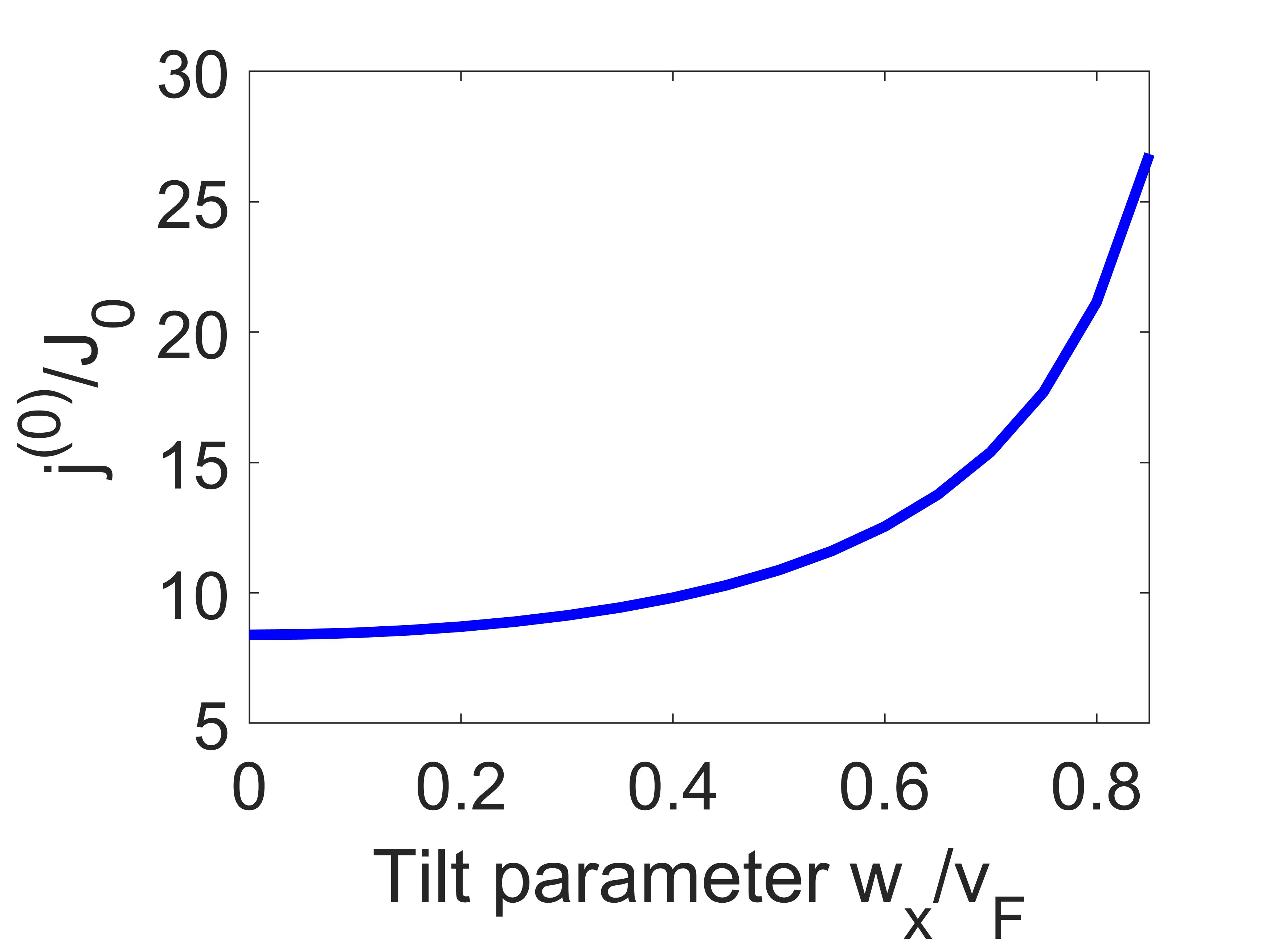
(a)

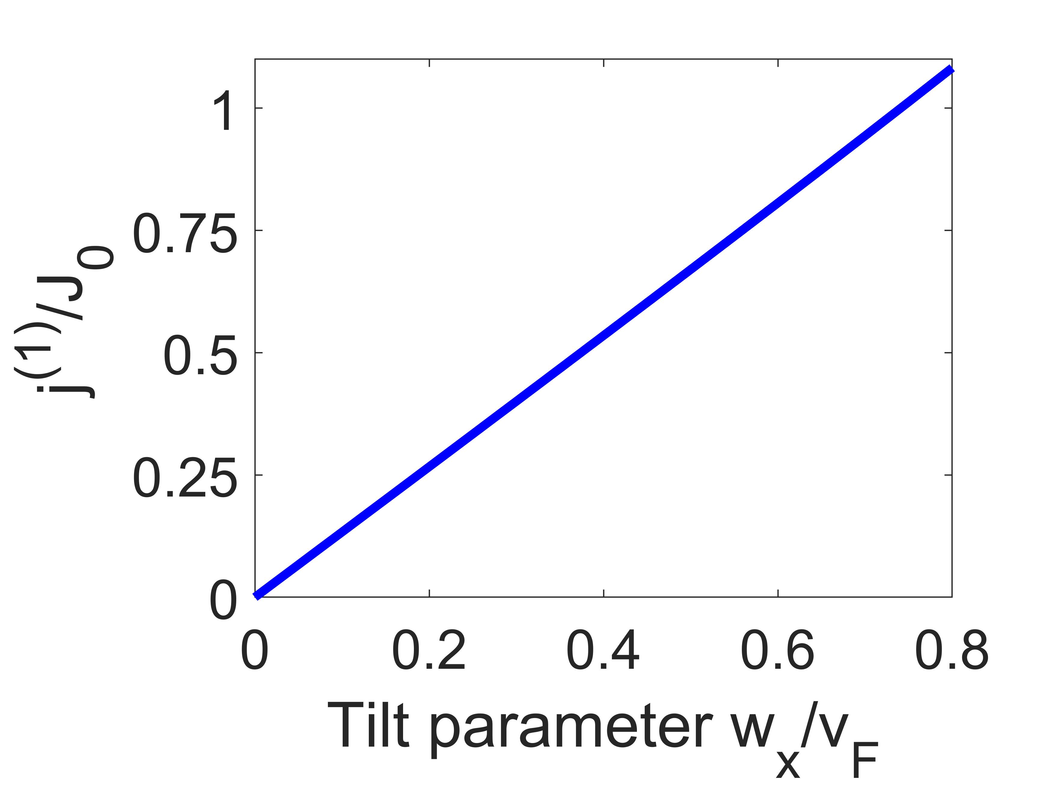
(b)

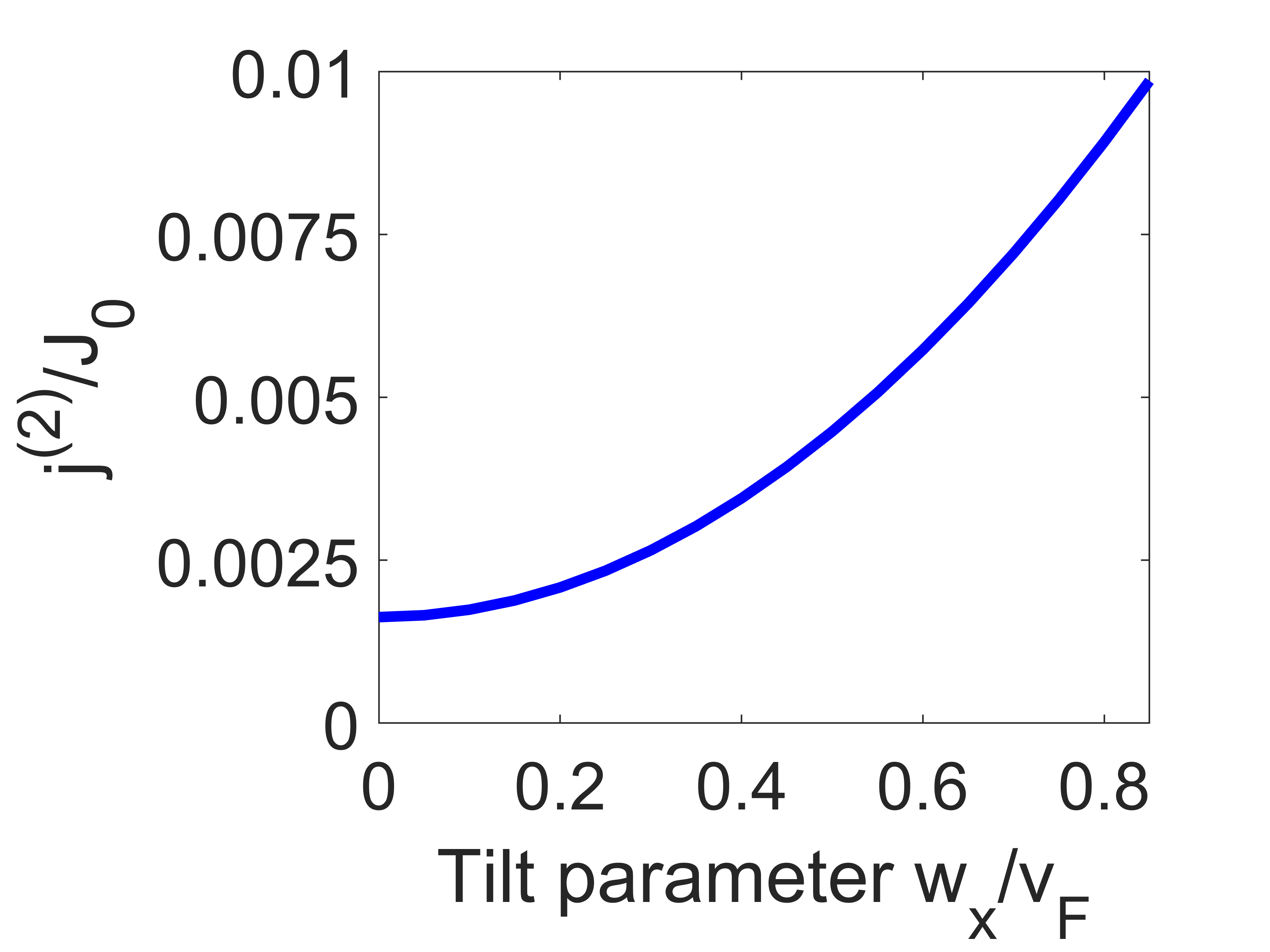
(c)

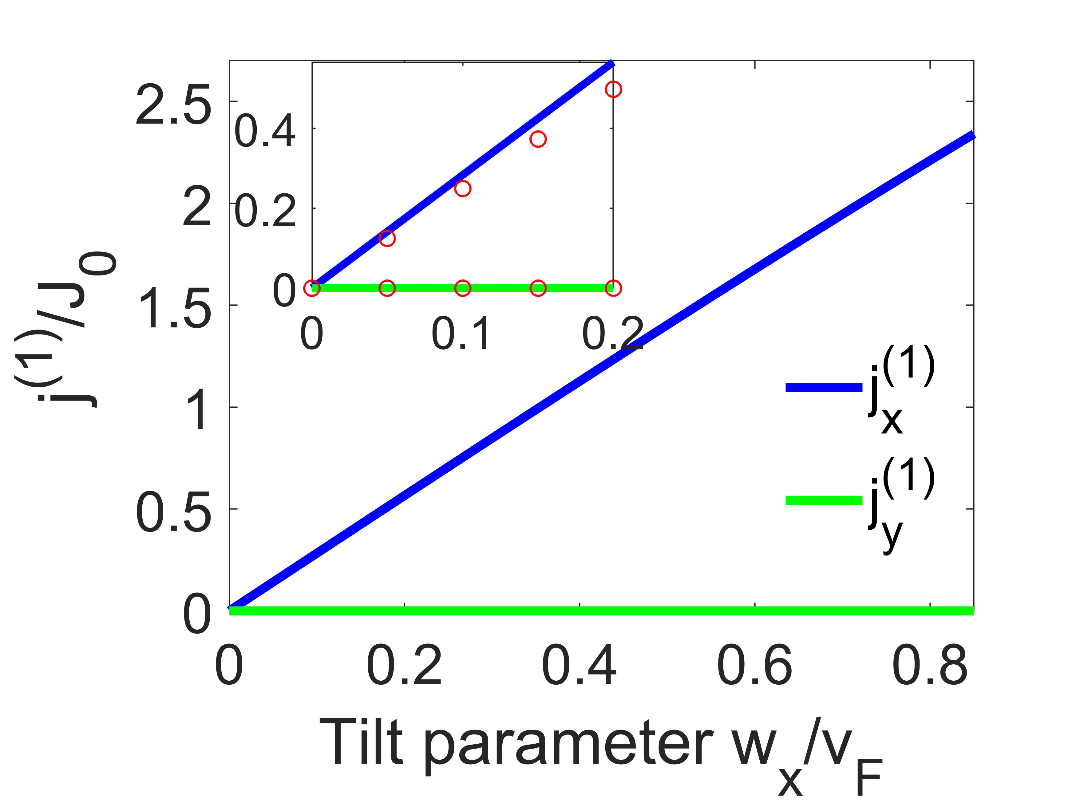
(d)

Figure 2: (Color online) (a)-(c), Plot of longitudinal components of current density $\mathbf{j}^{(0)}$, $\mathbf{j}^{(1)}$ and $\mathbf{j}^{(2)}$ with respect to $x$-component of tilt ($\text{w}_{x}$) when electric field $\mathbf{E}\parallel(\hat{x}+\hat{z})$. We use $J_{0}=\sigma_{0}|\mathbf{E}|$. (d) Plot of $x$ and $y$ components of $\mathbf{j}^{(1)}$ with respect to $x$-component of tilt $\text{w}_{x}$ when $\mathbf{E}||\mathbf{B}||\hat{z}$. Inset: Comparison with the analytical results (red circle), which are in close agreement with the numerical results at the small tilt limit.

Small tilt limit ($|\mathbf{w}|\ll v_{F}$): For small tilt, we expand Eqs. (6), (7) and (II) to the first order in $\mathbf{w}$ using $|\mathbf{v_{k}}|\approx v_{F}+(\hat{\mathrm{k}}\cdot\mathbf{w})+\mathcal{O}\left(|\mathbf{w}|^{2}\right)$. The presence of a finite tilt to the energy dispersion changes the shape of the Fermi surface (FS). However, in the small tilt limit, one can neglect this change and assume the shape of the FS to be spherical. We also consider the low-temperature limit such that we can approximate the distribution function $f^{0}$ to be the step function $\theta(\epsilon-\epsilon_{F})$ and consequently $\partial f^{0}/\partial\epsilon$ can be replaced by a Dirac delta function given by $\delta(\epsilon-\epsilon_{F})$ (note that most of the experimental transport measurements on WSMs are done at low temperatures at which this approximation is valid). Without loss of any generality, we choose the $z$-axis to be aligned along the magnetic field ($\mathbf{B}=B\hat{z}$) and that $\mathbf{w}$ and $\mathbf{B}$ lie in the same plane (Fig. 1(b)). Choosing the plane to be the $x$-$z$ plane, we write, $\mathbf{w}=\text{w}_{\text{{x}}}\hat{x}+\text{w}_{z}\hat{z}$ ($\text{w}_{x}$ and $\text{w}_{z}$ are the components of tilt and $\hat{x}$ and $\hat{z}$ are unit vectors along $x$ and $z$-axis ). Under the above assumptions, we calculate the current densities for a pair of Weyl nodes with opposite chirality to the first order in tilt and to the various orders in magnitude of the magnetic field $B$. While doing so we considered two distinct cases: (I) the tilt changes sign between the valleys with opposite chirality i.e. $\mathbf{w}_{\chi}=\chi\mathbf{w}$, and (II) the sign of the tilt remains unchanged in the two valleys i.e. $\mathbf{w}_{\chi}=\mathbf{w}$.

Case (a): In the small tilt limit, the current density can be evaluated analytically derived from the integrals in Eqs. (6)-(II) with $\mathbf{E}$ is chosen to be along $\parallel(\hat{x}+\hat{z})$. The current density of different orders in $B$ is given by (see the Supplemental Information for more details on the derivation):

$$\mathbf{j}^{(0)} =\frac{8\pi}{3}\sigma_{0}\mathbf{E},$$ (9)

$$\mathbf{j}^{(1)} =\frac{4\pi}{15}\sigma_{0}c_{b}\left[18\left(\mathbf{E}\cdot\mathbf{B}\right)\mathbf{w}+19\left(\mathbf{E}\cdot\mathbf{w}\right)\mathbf{B}\right.$$

$$\left.+\hat{x}\left(\mathbf{E}\times\mathbf{w}\cdot\hat{y}\right)B-\hat{y}\left(\mathbf{E}\times\mathbf{w}\cdot\hat{x}\right)B\right],$$ (10)

$$\mathbf{j}^{(2)} =2\pi\sigma_{0}c_{b}^{2}\left(\frac{1}{3}\left(\mathbf{E}\cdot\mathbf{B}\right)\mathbf{B}+\frac{1}{15}\mathbf{E}\right).$$ (11)

Interestingly, the first-order term is non-vanishing only in the presence of tilt, while the zeroth and second-order terms are independent of the tilt. This tilt dependence can be understood from the following argument. The anisotropic tilt appears in the integrals in Eqs. (6) to (II) because of the dependence of the group velocity $\mathbf{v_{k}}$ on tilt. In the case of both $\mathbf{j}^{(0)}$ and $\mathbf{j}^{(2)}$ all the terms in the integral are even in $\mathbf{k}$ in absence of tilt. However, in the presence of the dispersion tilt, these terms (to the first order in tilt) become odd in $\mathbf{k}$ i.e. the integrals change sign as one goes from $\mathbf{k}$ to $-\mathbf{k}$, and, as a consequence, vanish after integration over the FS (which is taken to be spherical). Conversely, for $\mathbf{j}^{(1)}$, all the terms in the current integral up to the first order in tilt are even in $\mathbf{k}$, and hence integration over the FS is not necessarily zero.

To understand the dependence of tilt on the current, we consider the implications of Eq. (10). We consider two particular cases, first, $\mathbf{E}\parallel\mathbf{B}$ i.e. the measurement set-up for longitudinal magnetoconductivity and second, $\mathbf{E}\perp\mathbf{B}$ i.e. the usual Hall measurement set-up. In the first case, i.e. for $\mathbf{E}\parallel\mathbf{B}\parallel\hat{z}$, we obtain,

$$\mathbf{j}^{(1)} =\sigma_{0}c_{b}\frac{4\pi}{15v_{F}}\left(19B\mathbf{w}+18\mathrm{w}_{z}\mathbf{B}\right)E.$$ (12)

Clearly, the current density has components not only along the direction of the magnetic field but also along the tilt directions. As a consequence, we have current transverse to the external electric field in the $x$-$z$ plane (the plane containing the tilt vector), i.e., $\mathbf{j}_{x}^{(1)}=\hat{x}\left(4\pi/15v_{F}\right)\sigma_{0}c_{b}\left(19|\mathbf{E}|B\text{w}_{x}\right)$ but no transverse current density perpendicular to that plane, i.e., $\mathbf{j}_{y}^{(1)}=0$.

Note that in the case of the longitudinal magneto-conductivity set up i.e. when $\mathbf{E}\parallel\mathbf{B}$, one usually obtains only the longitudinal component of current density since the Lorentz force is zero. However, in this case, we obtain non-zero transverse conductivity in the presence of tilt and Berry curvature. This unusual transverse signal should be readily measurable in this measurement set-up as one does not need to take into account the background Lorentz force induced Hall current. The tilt is a material-specific parameter whose direction and magnitude can, in principle, be determined from the band structure. If these tilt parameters are known, then our model can provide a prediction of the Berry curvature induced current. Numerically, from the plot in Fig. 2(d), we predict a planar Hall (PH) conductivity of $14.79$ $\text{oh}\text{m}^{-1}\text{m}^{-1}$ for a tilt value $\text{w}_{x}=0.1$ along the $x$-direction for Type-I WSM, and $14.21$ $\text{oh}\text{m}^{-1}\text{m}^{-1}$ for a tilt $\text{w}_{x}=1.6$ for Type-II WSM (plot is in the Supplemental).

Similarly, for the $\mathbf{E}\perp\mathbf{B}$ set-up, we derive the analytical expression for current in the small tilt limit to be,

$$\mathbf{j}^{(1)} =\frac{4\pi}{15}\sigma_{0}c_{b}\left[19\left(\mathbf{E}\cdot\mathbf{w}\right)\mathbf{B}-\left(\mathbf{B}\cdot\mathbf{w}\right)\mathbf{E}\right].$$ (13)

From above, we see that the current density has no component along the conventional Hall direction (i.e. parallel to $\mathbf{E}\times\mathbf{B}$). However, there is a non-zero planar Hall (PH) signal. In general, the PH effect is defined as the transverse current in the plane containing the electric and magnetic fields (i.e. along $\mathbf{E}\times(\mathbf{E}\times\mathbf{B})$ direction) when these fields are not parallel to each other. In our particular scenario, the PH current is parallel to $\mathbf{B}$ and is given by $\mathbf{j}_{PH}^{(1)}=\left(4\pi/15v_{F}\right)\sigma_{0}c_{b}19\left(\mathbf{E}\cdot\mathbf{w}\right)\mathbf{B}$.

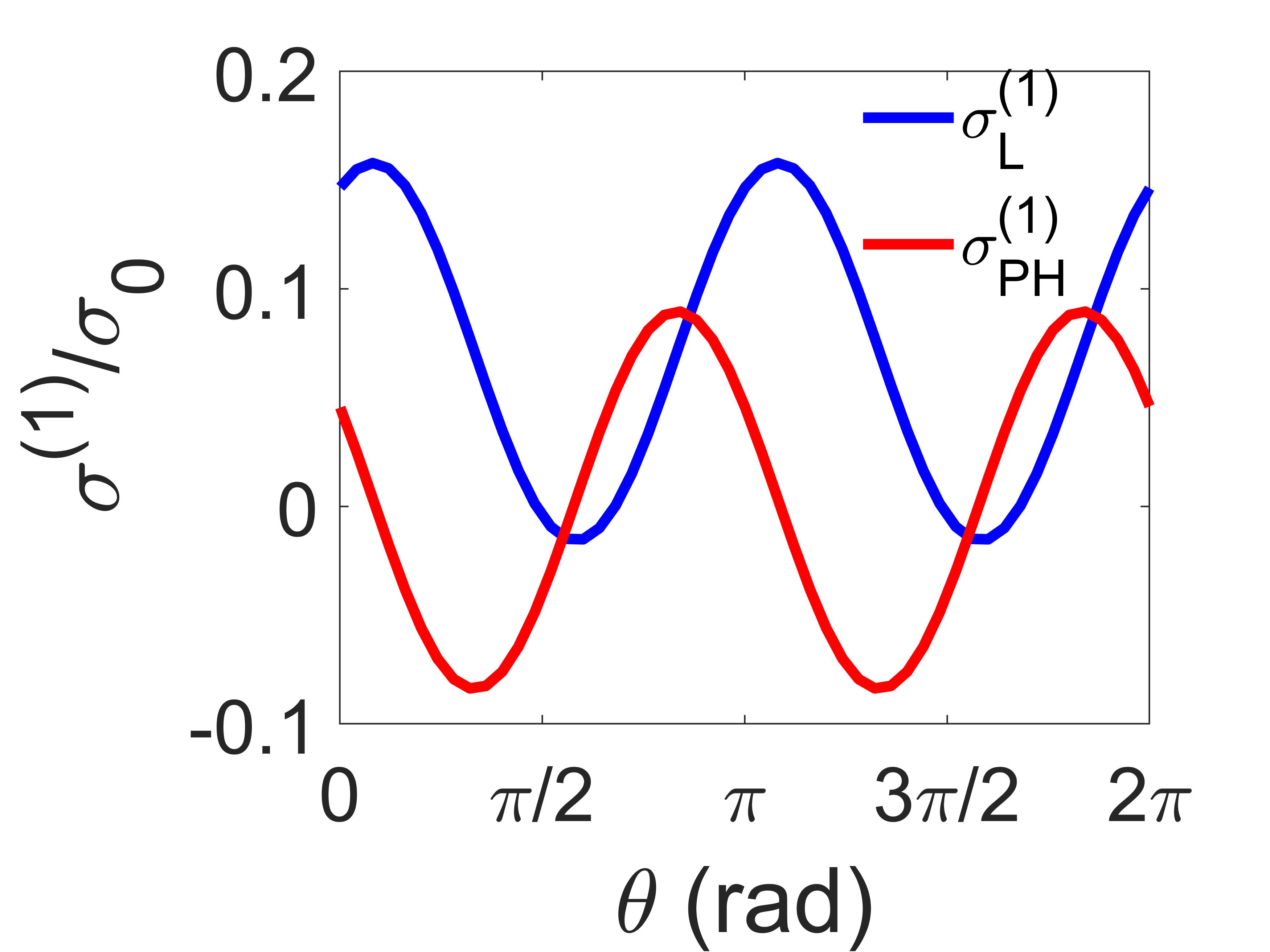
(a)

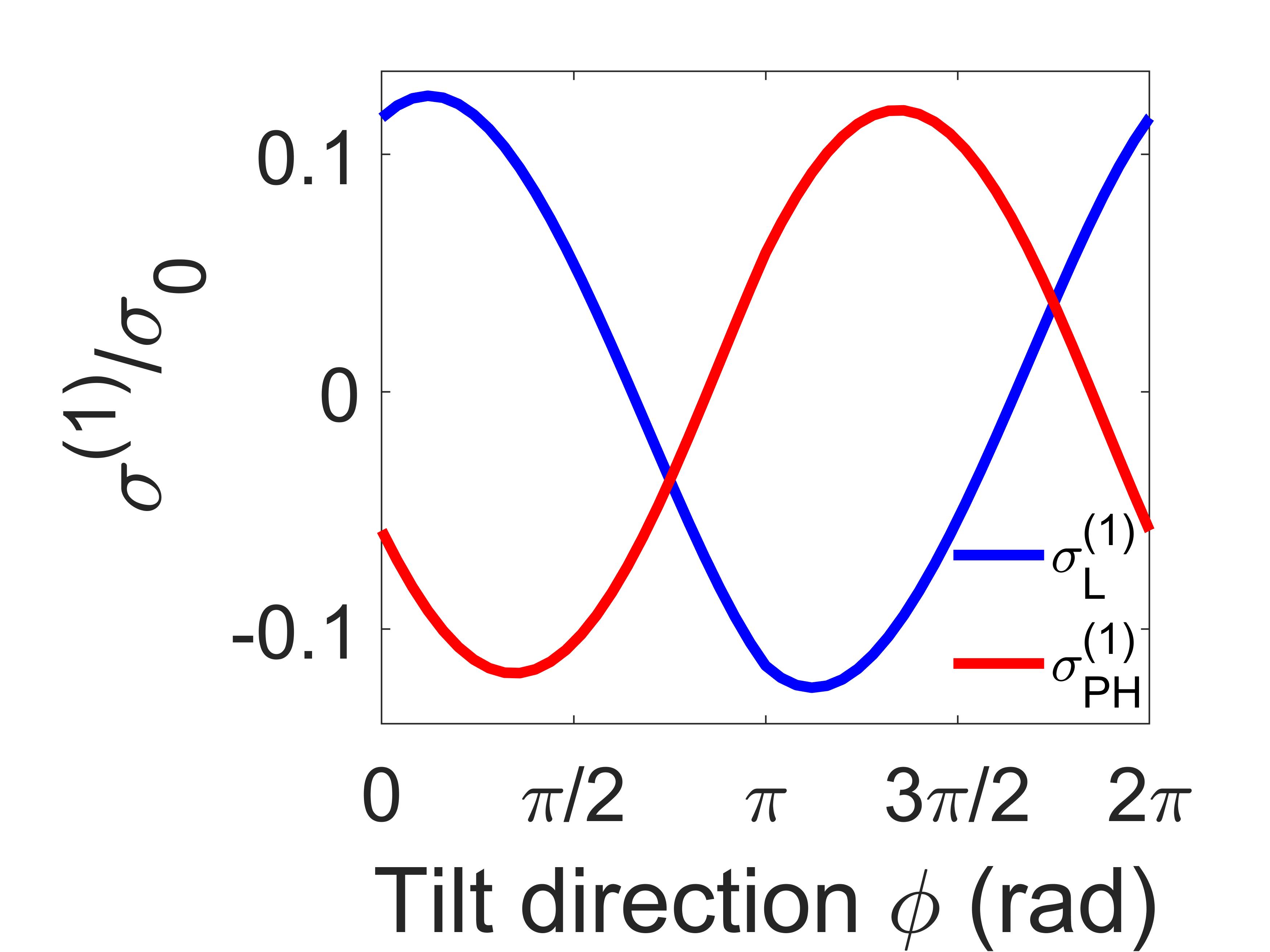
(b)

Figure 3: (Color online) Plot of longitudinal (blue) and PH (red) components of $\mathbf{j}^{(1)}$ with respect to (a) $\theta$, the angle between the electric and magnetic fields, and (b) with respect to the tilt direction $\phi$.

Arbitrary tilt strength: The analytical current density expressions derived in the previous section holds only in the small tilt limit. For arbitrarily large tilt strength, we calculate the conductivity numerically based on equations (6), (7), (II). In our numerical calculations, we assume the characteristic collision time to be $\tau=10^{-13}$ s Zhang2016 ; Huang2015 and Fermi energy $\epsilon_{F}=0.1$ eV. We set the magnetic field to be 3 T, electric field to be $10^{8}$ V/m and the temperature $T=30$ K. With these parameter values we have $\sigma_{0}=52.84$ $\text{Ohm}^{-1}\text{m}^{-1}$. In Fig. 2 (a), (b) and (c), we plot the longitudinal components of the zeroth, first and second-order terms of the current density as a function of the dispersion tilt in the $x$-direction, i.e., $\text{w}_{x}$ ($\mathrm{w}_{z}=0$) when the electric field direction is chosen arbitrarily to be $\mathbf{E}\parallel(\hat{x}+\hat{z})$ (i.e. $\mathbf{E}$ lies in the plane containing $\mathbf{w}$ and $\mathbf{B}$). At small tilt, the zeroth $j^{(0)}$ and second-order term $j^{(2)}$ does not change appreciably with the tilt, confirming our analytical prediction that the two terms are independent of the tilt at the small tilt limit (Eqs. (9) and (11)). However, at sufficiently large tilt ($|\mathbf{w}|/v_{F}>0.2$), the response of those terms to the tilt becomes non-linear. By contrast, the first-order term $j^{(1)}$ varies linearly with the tilt parameter $\text{w}_{x}$ even at large tilt, a response that is in line with the analytical result of Eq. (10).

Note that all the various orders of current density show an increasing trend with the tilt parameter. A possible reason for this increase of current density is due to the fact that the magnitude of the group velocity $\mathbf{v_{k}}$ and the area of the FS both increase with the tilt strength. Although the addition of a tilt term in the Hamiltonian does not change the topological properties of the WSMs, it does change the energy dispersion and as a consequence the shape of the FS. For a Type-I WSM, the shape of FS is ellipsoid where the axis of the ellipsoid is determined by the tilt direction while for Type-II, the shape becomes hyperboloid. As the total current density is calculated by integrating over the FS, the shape and size of the FS have an influence on the current density. The effect of the FS geometry is even more prominent in the case of Type-II WSM (this is discussed at the end of this section based on results given in the Supplemental).

Next, we evaluate numerically the transverse current in the longitudinal magneto-conductivity setup, i.e., $\mathbf{E}\parallel\mathbf{B}\parallel\hat{z}$. In Fig. 2(d), we plot the perpendicular components of $\mathbf{j}^{(1)}$ corresponding to this set up, both in the in-plane ($x$-$z$ plane) and out-of-plane directions, as a function of the tilt parameter $\text{w}_{x}$. In the inset, the numerical results are compared with the analytical prediction of Eq. (12), showing good agreement at the small tilt values. It can be seen that the in-plane transverse component of current density increases linearly with $\text{w}_{x}$ while the out-of-plane component is zero, both trends of which match that of the analytical form in Eq.(12).

The presence of the in-plane transverse current in Fig. 2(d) even in the longitudinal set up where the $\mathbf{E}$ and $\mathbf{B}$ fields are parallel to each other can be understood in terms of the group velocity $\mathbf{v}_{\mathbf{k}}$ in Eq. (7). In the absence of tilt $\mathbf{v}_{\mathbf{k}}\parallel\mathbf{k}\parallel\mathbf{\Omega}_{\mathbf{k}}$, and, thus the second and third terms are odd in $\mathbf{k}$ as a consequence of which the integration over FS is zero for those terms, resulting in the current being parallel to $\mathbf{B}$. However at finite tilt, $|\mathbf{v_{k}}|=v_{F}\hat{\mathrm{k}}+\mathbf{w}$, and as a result a component of the current density along the tilt direction appears. In our case, we considered $\mathbf{w}=\text{w}_{x}\hat{x}$ and thus we obtain a transverse current in the $x$-direction, which is also in accordance with our calculation in Eq. (12).

Next, we consider the longitudinal and PH current densities under varying the angle $\theta$ between the electric and magnetic fields, under varying tilt direction ( denoted by $\phi$). We express the tilt vector as $\mathbf{w}=|\mathbf{w}|(\cos\phi~{}\hat{x}+\sin\phi~{}\hat{z})$, where $\phi$ is the angle between the tilt vector and the $x$-axis. The electric field is chosen to lie on the $x$-$z$ plane, i.e., $\mathbf{E}=|\mathbf{E}|(\sin\theta~{}\hat{x}+\cos\theta~{}\hat{z})$. Substituting the expressions for $\mathbf{w}$ and $\mathbf{E}$ into Eq. (10), the angular dependence of the longitudinal and PH conductivities at the small tilt is given as,

$$\sigma^{(1)}_{L}=\frac{4\pi B|\mathbf{w}|}{15v_{F}}\left(19\sin(2\theta+\phi)+18\sin\phi\right),$$ (14)

and

$$\sigma^{(1)}_{PH}=\frac{4\pi B|\mathbf{w}|}{15v_{F}}19\cos(2\theta+\phi).$$ (15)

Clearly, the tilt introduces an additional anisotropy in both the conductivity terms. In Fig. 3(a), we plot both the longitudinal and PH conductivities with the variation of the field angle $\theta$ for a fix tilt direction of $\phi=\pi/3$ and magnitude of $|\mathbf{w}|=0.1$.

In Fig. 3(b) we plot the variation of both the longitudinal and PH conductivities with the variation of the tilt direction $\phi$, for a fixed angle between electric and magnetic fields ($\theta=\pi/3$). Note that because of the sinusoidal dependence on $\phi$, both current densities change sign, when the tilt direction is reversed, i.e., from $\phi$ to $(\phi+\pi)$. This behavior also matches with the analytical calculation in Eq. (12). Based on this, let us consider the PH current for different tilt configuration of the Dirac cone for a pair of WPs. Now, if, for a certain value of $\phi$, the tilt for a pair of WPs is given by $\mathbf{w}_{\pm}=\pm\mathbf{w}$ then the Dirac cones are tilted towards each other. Then for $(\phi+\pi)$, the tilt vector for the pair becomes $\mathbf{w}_{\pm}=\mp\mathbf{w}$, i.e., the cones are tilted outwards in k-space (see Fig. 1(c) and (d)) and the direction of the PH current is reversed. This suggests that one can control the PH current via tilt engineering. For example, if the dispersion tilt can be controlled by some external parameters such as strain, then one can achieve strain-induced switching of the PH current or voltage due to the reversal of the relative tilt between the dispersion cones at the two WPs.

Case (b): This case corresponds to the scenario where the tilt is uniform, i.e., when $\mathbf{w}_{\chi}=\mathbf{w}$ at all WPs. For this case, the current densities are given by, $\mathbf{j}^{(0)}=(8\pi/3)\sigma_{0}\mathbf{E},$ $\mathbf{j}^{(1)}=0,$ $\mathbf{j}^{(2)}=2\pi\sigma_{0}c_{b}^{2}\left(\frac{1}{3}\left(\mathbf{E}\cdot\mathbf{B}\right)\mathbf{B}+\frac{1}{15}\mathbf{E}\right).$ Specifically, in this case, the PH contribution from the two valleys would cancel out each other giving rise to zero net PH signal. The corresponding plots for the tilt dependence of the zeroth and second-order current densities are plotted in the Supplemental.

Type-II: For the Type-II WSMs ($|\mathbf{w}|>v_{F}$) the FS is open and adopts a hyperboloid configuration. Since, by definition, we are in the large tilt regime, no simple analytical expressions of the current densities can be obtained. Instead, we perform numerical calculations of the conductance in Type-II WSM from the integrations in Eqs. (6), (7) and (II) for different values of tilt parameter $\text{w}_{x}$. These numerical results are plotted in the Supplemental. Interestingly, we find similar trends in the current density compared to that of Type-I WSM, e.g., the current densities tend to increase with the tilt strength. More importantly, the tilt-induced PH signal is still present in the case of Type-II WSM.

IV Conclusion

Using a semiclassical approach, we analyze the magnetotransport of a WSM with Dirac cones that are tilted in the momentum space. We calculate the current density up to the second-order in the $B$-field strength and derive the analytical expression in the small tilt limit. The analytical predictions were verified by numerical calculations for arbitrary tilt values. In addition, we evaluate the planar Hall (PH) current when the magnetic field, electric field, and the tilt vector lies in the same plane. Both the longitudinal and PH conductivity can be controlled by tuning the direction and magnitude of the tilt parameter. A tilt-induced transverse current exists even when $\mathbf{E}\parallel\mathbf{B}$, where the conventional Hall current vanishes. This work is supported by the following grants: MOE Tier I (NUS Grant No. R-263-000-D66-114), MOE Tier II MOE2018-T2-2-117 (NUS Grant No. R-398-000-092-112) and NRF-CRP12-2013-01 (NUS Grant No. R-263-000-B30-281).

References

- [1] Shuichi Murakami. Phase transition between the quantum spin hall and insulator phases in 3d: emergence of a topological gapless phase. New Journal of Physics, 9(9):356, 2007.
- [2] Xiangang Wan, Ari M. Turner, Ashvin Vishwanath, and Sergey Y. Savrasov. Topological semimetal and fermi-arc surface states in the electronic structure of pyrochlore iridates. Phys. Rev. B, 83:205101, May 2011.
- [3] H. B. Nielsen and M. Ninomiya. The Adler-Bell-Jackiw anomaly and Weyl fermions in a crystal. Physics Letters B, 130:389–396, November 1983.
- [4] Frank Arnold, Chandra Shekhar, Shu-Chun Wu, Yan Sun, Ricardo Donizeth dos Reis, Nitesh Kumar, Marcel Naumann, Mukkattu O. Ajeesh, Marcus Schmidt, Adolfo G. Grushin, Jens H. Bardarson, Michael Baenitz, Dmitry Sokolov, Horst Borrmann, Michael Nicklas, Claudia Felser, Elena Hassinger, and Binghai Yan. Negative magnetoresistance without well-defined chirality in the weyl semimetal tap. Nature Communications, 7:11615 EP –, May 2016. Article.
- [5] Cai-Zhen Li, Li-Xian Wang, Haiwen Liu, Jian Wang, Zhi-Min Liao, and Da-Peng Yu. Giant negative magnetoresistance induced by the chiral anomaly in individual cd3as2 nanowires. Nature Communications, 6:10137 EP –, Dec 2015. Article.
- [6] Qiang Li, Dmitri E. Kharzeev, Cheng Zhang, Yuan Huang, I. Pletikosic, A. ?. V. Fedorov, R. ?. D. Zhong, J. ?. A. Schneeloch, G. ?. D. Gu, and T. Valla. Chiral magnetic effect in zrte5. Nature Physics, 12:550 EP –, Feb 2016.
- [7] Xiaochun Huang, Lingxiao Zhao, Yujia Long, Peipei Wang, Dong Chen, Zhanhai Yang, Hui Liang, Mianqi Xue, Hongming Weng, Zhong Fang, Xi Dai, and Genfu Chen. Observation of the chiral-anomaly-induced negative magnetoresistance in 3d weyl semimetal taas. Phys. Rev. X, 5:031023, Aug 2015.
- [8] Jun Xiong, Satya K. Kushwaha, Tian Liang, Jason W. Krizan, Max Hirschberger, Wudi Wang, R. J. Cava, and N. P. Ong. Evidence for the chiral anomaly in the dirac semimetal na3bi. Science, 350(6259):413–416, 2015.
- [9] Cheng-Long Zhang, Su-Yang Xu, Ilya Belopolski, Zhujun Yuan, Ziquan Lin, Bingbing Tong, Guang Bian, Nasser Alidoust, Chi-Cheng Lee, Shin-Ming Huang, Tay-Rong Chang, Guoqing Chang, Chuang-Han Hsu, Horng-Tay Jeng, Madhab Neupane, Daniel S. Sanchez, Hao Zheng, Junfeng Wang, Hsin Lin, Chi Zhang, Hai-Zhou Lu, Shun-Qing Shen, Titus Neupert, M. Zahid Hasan, and Shuang Jia. Signatures of the adler-bell-jackiw chiral anomaly in a weyl fermion semimetal. Nature Communications, 7:10735 EP –, Feb 2016. Article.
- [10] M. O. Goerbig, J.-N. Fuchs, G. Montambaux, and F. Piéchon. Tilted anisotropic dirac cones in quinoid-type graphene and . Phys. Rev. B, 78:045415, Jul 2008.
- [11] Alexey A. Soluyanov, Dominik Gresch, Zhijun Wang, QuanSheng Wu, Matthias Troyer, Xi Dai, and B. Andrei Bernevig. Type-ii weyl semimetals. Nature, 527:495 EP –, Nov 2015.
- [12] Su-Yang Xu, Nasser Alidoust, Guoqing Chang, Hong Lu, Bahadur Singh, Ilya Belopolski, Daniel S. Sanchez, Xiao Zhang, Guang Bian, Hao Zheng, Marious-Adrian Husanu, Yi Bian, Shin-Ming Huang, Chuang-Han Hsu, Tay-Rong Chang, Horng-Tay Jeng, Arun Bansil, Titus Neupert, Vladimir N. Strocov, Hsin Lin, Shuang Jia, and M. Zahid Hasan. Discovery of lorentz-violating type ii weyl fermions in laalge. Science Advances, 3(6), 2017.
- [13] Ke Deng, Guoliang Wan, Peng Deng, Kenan Zhang, Shijie Ding, Eryin Wang, Mingzhe Yan, Huaqing Huang, Hongyun Zhang, Zhilin Xu, Jonathan Denlinger, Alexei Fedorov, Haitao Yang, Wenhui Duan, Hong Yao, Yang Wu, Shoushan Fan, Haijun Zhang, Xi Chen, and Shuyun Zhou. Experimental observation of topological fermi arcs in type-ii weyl semimetal mote2. Nature Physics, 12:1105 EP –, Sep 2016.
- [14] Peng Li, Yan Wen, Xin He, Qiang Zhang, Chuan Xia, Zhi-Ming Yu, Shengyuan A. Yang, Zhiyong Zhu, Husam N. Alshareef, and Xi-Xiang Zhang. Evidence for topological type-ii weyl semimetal wte2. Nature Communications, 8(1):2150, 2017.
- [15] Timothy M. McCormick, Itamar Kimchi, and Nandini Trivedi. Minimal models for topological weyl semimetals. Phys. Rev. B, 95:075133, Feb 2017.
- [16] Zhi-Ming Yu, Yugui Yao, and Shengyuan A. Yang. Predicted unusual magnetoresponse in type-ii weyl semimetals. Phys. Rev. Lett., 117:077202, Aug 2016.
- [17] T. E. O’Brien, M. Diez, and C. W. J. Beenakker. Magnetic breakdown and klein tunneling in a type-ii weyl semimetal. Phys. Rev. Lett., 116:236401, Jun 2016.
- [18] A. A. Zyuzin and R. P. Tiwari. Intrinsic anomalous hall effect in type-ii weyl semimetals. JETP Letters, 103(11):717–722, Jun 2016.
- [19] Yago Ferreiros, A. A. Zyuzin, and Jens H. Bardarson. Anomalous nernst and thermal hall effects in tilted weyl semimetals. Phys. Rev. B, 96:115202, Sep 2017.
- [20] Subhodip Saha and Sumanta Tewari. Anomalous nernst effect in type-ii weyl semimetals. The European Physical Journal B, 91(1):4, Jan 2018.
- [21] S. P. Mukherjee and J. P. Carbotte. Absorption of circular polarized light in tilted type-i and type-ii weyl semimetals. Phys. Rev. B, 96:085114, Aug 2017.
- [22] Da Ma, Hua Jiang, Haiwen Liu, and X. C. Xie. Planar hall effect in tilted weyl semimetals. Phys. Rev. B, 99:115121, Mar 2019.
- [23] S. Nandy, Girish Sharma, A. Taraphder, and Sumanta Tewari. Chiral anomaly as the origin of the planar hall effect in weyl semimetals. Phys. Rev. Lett., 119:176804, Oct 2017.
- [24] Nitesh Kumar, Satya N. Guin, Claudia Felser, and Chandra Shekhar. Planar hall effect in the weyl semimetal gdptbi. Phys. Rev. B, 98:041103, Jul 2018.
- [25] D. T. Son and B. Z. Spivak. Chiral anomaly and classical negative magnetoresistance of weyl metals. Phys. Rev. B, 88:104412, Sep 2013.
- [26] Ganesh Sundaram and Qian Niu. Wave-packet dynamics in slowly perturbed crystals: Gradient corrections and berry-phase effects. Phys. Rev. B, 59:14915–14925, Jun 1999.
- [27] Di Xiao, Ming-Che Chang, and Qian Niu. Berry phase effects on electronic properties. Rev. Mod. Phys., 82:1959–2007, Jul 2010.
- [28] Shin-Ming Huang, Su-Yang Xu, Ilya Belopolski, Chi-Cheng Lee, Guoqing Chang, BaoKai Wang, Nasser Alidoust, Guang Bian, Madhab Neupane, Chenglong Zhang, Shuang Jia, Arun Bansil, Hsin Lin, and M. Zahid Hasan. A weyl fermion semimetal with surface fermi arcs in the transition metal monopnictide taas class. Nature Communications, 6:7373 EP –, Jun 2015. Article.