Stability Analysis of Infinite-dimensional Event-triggered and Self-triggered Control Systems with Lipschitz Perturbations

Abstract.

This paper addresses the following question: “Suppose that a state-feedback controller stabilizes an infinite-dimensional linear continuous-time system. If we choose the parameters of an event/self-triggering mechanism appropriately, is the event/self-triggered control system stable under all sufficiently small nonlinear Lipschitz perturbations?” We assume that the stabilizing feedback operator is compact. This assumption is used to guarantee the strict positiveness of inter-event times and the existence of the mild solution of evolution equations with unbounded control operators. First, for the case where the control operator is bounded, we show that the answer to the above question is positive, giving a sufficient condition for exponential stability, which can be employed for the design of event/self-triggering mechanisms. Next, we investigate the case where the control operator is unbounded and prove that the answer is still positive for periodic event-triggering mechanisms.

Masashi Wakaiki^∗

Graduate School of System Informatics, Kobe University

Nada, Kobe, Hyogo 657-8501, Japan

Hideki Sano

Graduate School of System Informatics, Kobe University

Nada, Kobe, Hyogo 657-8501, Japan

(Communicated by the associate editor name)

1. Introduction

In this paper, we study event/self-triggered control for infinite-dimensional systems. As the time-discretization of control systems, periodic sampling and control-updating are widely used. Various problems on periodic sampled-data control have been studied for infinite-dimensional systems; for example, stabilization [34, 29, 24, 22, 15, 14, 38, 21], robustness analysis of continuous-time stabilization with respect to periodic sampling [30, 23, 31], and output regulation [25, 19, 17, 18, 37]. Event/self-triggering mechanisms are other time-discretization methods, which send measurements and update control inputs when they are needed. In event-triggered control systems, a sensor monitors the plant output and determines when it sends the data to a controller (Figure 1). On the other hand, in self-triggered control systems, the controller computes times at which the sensor transmits the data to the controller (Figure 2). The major difference is that the current output can be used to determine transmission times in event-triggered control systems but not in self-triggered control systems. Therefore, in the state-feedback case where we denote by $x(t)$ the state at time $t\geq 0$, the transmission times $\{t_{k}\}_{k\in\mathbb{N}_{0}}$ of event-triggered control systems are typically computed in the form $t_{k+1}=\inf\big{\{}t>t_{k}:F_{\rm e}\big{(}x(t),x(t_{k})\big{)}>0\big{\}}$ and those of self-triggered control systems are in the form $t_{k+1}=t_{k}+F_{\rm s}\big{(}x(t_{k})\big{)}$ for some functions $F_{\rm e}$ and $F_{\rm s}$.

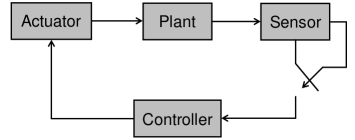
Figure 1. Event-triggered control system.

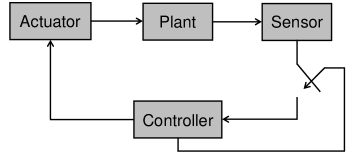
Figure 2. Self-triggered control system.

Event/self-triggered control has been an area of intense research, starting from the seminal works of Tabuada [33], Wang and Lemmon [39], Anta and Tabuada [1] for finite-dimensional systems. Adaptation of sampling periods in sampled-data systems is a topic close to event/self-triggered control, which has been also explored in [12] for finite-dimensional systems. Event-triggered control methods have been extended to some classes of infinite-dimensional systems, e.g., systems with output delays and packet losses [20], first-order hyperbolic systems [6, 7], second-order hyperbolic systems [3], second-order parabolic systems [13, 32, 16], and abstract linear evolution equations [36]. However, relatively little work has been done on self-triggered control for infinite-dimensional systems, compared with event-triggered control.

We consider the following system with state space $X$ and input space $U$ (both Hilbert spaces):

$$\dot{x}(t)=Ax(t)+Bu(t)+\phi\big{(}x(t)\big{)},\quad t\geq 0;\qquad x(0)=x^{0}\in X,$$ (1)

where $A$ is the generator of a strongly continuous semigroup $T(t)$ on $X$, the control operator $B$ is a bounded linear operator from $U$ to the extrapolation space $X_{-1}$ associated with $T(t)$ (see the notation section for the definition of the extrapolation space $X_{-1}$), and the perturbation $\phi$ is a nonlinear operator on $X$ satisfying $\phi(0)=0$ and the Lipschitz condition

$$\|\phi(\xi_{1})-\phi(\xi_{2})\|\leq L\|\xi_{1}-\xi_{2}\|\qquad\forall\xi_{1},\xi_{2}\in X$$

for some Lipschitz constant $L\geq 0$. We call the control operator $B$ in (1) bounded if $B$ maps boundedly from $U$ into $X$. Otherwise, we call $B$ unbounded.

Choose a bounded linear operator $F$ from $X$ to $U$ such that the state-feedback controller $u(t)=Fx(t)$ exponentially stabilizes the linear system $\dot{x}(t)=Ax(t)+Bu(t)$, that is, the strongly continuous semigroup generated by $A+BF$ is exponentially stable. For the infinite-dimensional system (1), we here implement an event/self-triggering controller, which is given by

$$u(t)=Fx(t_{k}),\quad t_{k}\leq t<t_{k+1},~{}k\in\mathbb{N}_{0},$$ (2)

where $\{t_{k}\}_{k\in\mathbb{N}_{0}}$ is determined by a certain event/self-triggering mechanism. If we appropriately choose the parameters of the event/self-triggering mechanism, then the inter-event times $t_{k+1}-t_{k}$ can be small. Therefore, we would expect intuitively that the event/self-triggered controller (2) exponentially stabilizes the system (1) for all perturbations with sufficiently small Lipschitz constants $L$. The main objective of this paper is to show that this intuition is correct.

In addition to stabilization, the minimum inter-event time, $\inf_{k\in\mathbb{N}_{0}}(t_{k+1}-t_{k})$, needs to be strictly positive. Otherwise, data transmissions might occur infinitely fast, which cannot be executed in practical implementation. This is an example of Zeno behavior studied in the context of hybrid systems; see, e.g., [9]. In the infinite-dimensional case, a careful treatment of the minimum inter-event time is required even for state-feedback control. In fact, for finite-dimensional linear systems, if we use the following standard event-triggering mechanism proposed in [33]:

$$t_{k+1}=\inf\{t>t_{k}:\|x(t_{k})-x(t)\|>\varepsilon\|x(t)\|\},\quad k\in\mathbb{N}_{0},~{}\varepsilon>0,$$ (3)

then for every threshold $\varepsilon>0$, there exists $\theta>0$ such that $\inf_{k\in\mathbb{N}_{0}}(t_{k+1}-t_{k})\geq\theta$ for all $x^{0}\in X$; see Corollary IV.1 of [33]. However, for infinite-dimensional linear systems, the same mechanism may not guarantee that the minimum inter-event time is bounded from below by a positive constant as shown in Examples 3.1 and 3.2 in [36].

The important assumption of this paper is that the feedback operator $F$ is compact, which is used for two purposes. First, we guarantee the strict positiveness of inter-event times, using the compactness of the feedback operator. Second, this assumption is employed to prove the existence of the mild solution of the evolution equation (1) and (2) in the unbounded control case.

We start with the case in which $B$ is bounded. In the previous work [36], the following event-triggering mechanism has been considered for the system (1) in the unperturbed case $\phi\equiv 0$:

$$t_{k+1} =\min\big{\{}t_{k}+\tau_{\max},~{}\inf\{t>t_{k}:\|Fx(t_{k})-Fx(t)\|_{U}>\varepsilon\|x(t_{k})\|\}\big{\}}$$ (4)

for $k\in\mathbb{N}_{0}$, where $\tau_{\max}>0$ is an upper bound of inter-event times. The self-triggering mechanism we propose in this paper is based on (4). Before describing it, we briefly explain two different points of the event-triggering mechanism (4) from the standard one (3).

First, the mechanism (4) has the upper bound $\tau_{\max}$ of inter-event times. Since $\|x(t_{k})\|$ is used for the estimation of the implementation-induced error $\|Fx(t_{k})-Fx(t)\|_{U}$ in the mechanism (4), exponential convergence is not guaranteed unless we set an upper bound of inter-event times. The exponential stability of the unperturbed event-triggered control system is achieved for every $\tau_{\max}>0$ under some condition on the threshold $\varepsilon$, although the decay rate becomes small as $\tau_{\max}$ increases; see Theorem 4.1 in [36].

Second, the implementation-induced error of the input, $\|Fx(t_{k})-Fx(t)\|_{U}$, is used in (4). As in the case of the mechanism (3), there exists an infinite-dimensional systems such that an event-triggering mechanism using the condition $\|x(t_{k})-x(t)\|>\varepsilon\|x(t_{k})\|$ does not guarantees that the minimum inter-event time is bounded from below by positive constant; see Example 3.1 in [36]. However, it has been shown in Theorem 3.6 of [36] that the minimum inter-event time of the mechanism (4) is strictly positive if the feedback operator $F$ is compact.

Event-triggering mechanisms using the feedback operator $F$ are not practical in some situations. This is the main motivation of the extension of (4) to a self-triggering mechanism. It is reasonable that the controller uses the mechanism (4) for the computation of transmission times at which the controller sends the control input to the actuator. However, it makes little sense that the sensor uses the mechanism (4) in the situation where the sensor and the controller are separated. Indeed, since the control input is computed in the mechanism (4), the sensor may directly transmit the control input to the actuator without going through the controller; see also the discussion in Section VII-B of [33].

For the bounded control case, we propose the following self-triggering mechanism:

$$t_{k+1} =t_{k}+\min\big{\{}\tau_{\max},~{}\inf\{\tau>0:\alpha_{L,\varepsilon}(x(t_{k}),\tau)\geq\varepsilon\|x(t_{k})\|\}\big{\}}$$ (5)

for $k\in\mathbb{N}_{0}$, where $\alpha_{L,\varepsilon}:X\times\mathbb{R}_{+}\to\mathbb{R}_{+}$ is a certain function depending on $L$ and $\varepsilon$; see Section 2.2 for details. Instead of monitoring the state $x(t)$ continuously, the self-triggering mechanism (5) predicts it to estimate $\|Fx(t_{k})-Fx(t)\|_{U}$, by using the nominal linear model $(T(t),B,F)$, the Lipschitz constant $L$, and the latest transmitted state $x(t_{k})$. Consequently, the self-triggering mechanism (5) can be implemented in the controller. The function $\alpha_{L,\varepsilon}$ is defined so that

$$\|Fx(t_{k})-Fx(t)\|_{U}\leq\alpha_{L,\varepsilon}(x(t_{k}),t-t_{k})$$

holds for every $t\in[t_{k},t_{k+1})$ and $k\in\mathbb{N}_{0}$. Therefore, under the self-triggering mechanism (5), we obtain

$$\|Fx(t_{k})-Fx(t)\|_{U}\leq\varepsilon\|x(t_{k})\|$$

for every $t\in[t_{k},t_{k+1})$ and $k\in\mathbb{N}_{0}$ as under the event-triggering mechanism (4). We show the strict positiveness of inter-event times and provide a sufficient condition for the exponential stability of the self-triggered control system.

Another solution to avoid the use of the feedback operator $F$ in the sensor is the following event-triggering mechanisms:

$$t_{k+1}=\min\big{\{}t_{k}+\tau_{\max},~{}\inf\{t>t_{k}+\tau_{\min}:\|x(t_{k})-x(t)\|>\varepsilon\|x(t_{k})\|\}\big{\}}$$ (6)

for $k\in\mathbb{N}_{0}$, where $\tau_{\min}\in(0,\tau_{\max})$ is a prespecified lower bound of inter-event times. The event-triggering mechanism (6) is based on the one studied in [11] for finite-dimensional systems. The difficulty here is that the event-triggering mechanism (6) does not guarantee that the error $\|x(t_{k})-x(t_{k}+\tau)\|$ is small for $0<\tau<\tau_{\min}$. However, we show that if the lower bound $\tau_{\min}$ is chosen appropriately, then exponential stability is preserved under the event-triggering mechanism (6) for all sufficiently small Lipschitz constants $L>0$ and thresholds $\varepsilon\geq 0$. For the unperturbed case $\phi\equiv 0$, we also provide a simple sufficient condition for exponential stability, in which the upper bound $\tau_{\max}$ of inter-event times does not appear as in the case of the event-triggering mechanism (4). It is worthwhile noticing that the stability analysis under the event-triggering mechanism (6) is new even without Lipschitz perturbations.

Next we investigate the case in which $B$ is unbounded. As in the unperturbed case $\phi\equiv 0$ in Section 5.2 of [36], we apply the following periodic event-triggering mechanism:

$$t_{k+1}:=\min\big{\{}t_{k}+\ell_{\max}h,~{}\min\{\ell h>t_{k}:\|x(t_{k})-x(\ell h)\|>\varepsilon\|x(t_{k})\|,~{}\ell\in\mathbb{N}\}\big{\}},$$ (7)

where $h>0$ is a sampling period and $\ell_{\max}\in\mathbb{N}$ determines an upper bound of inter-event times. The periodic event-triggering mechanism has been studied for finite-dimensional linear systems in [10] and then has been extended to finite-dimensional nonlinear Lipschitz systems in [8]. Compared with the above mechanisms (3), (4), and (6), the periodic event-triggering mechanism (7) behaves in a more time-triggering fashion, because the condition is verified only periodically. This periodic aspect leads to several benefits. First, the minimum inter-event time is bounded from below by $h$. Second, the sensor needs to monitor the state and check the condition only at sampling times, and hence the periodic event-triggering mechanism (7) is more suitable for practical implementations.

In the unbounded control case, we begin by showing that a mild solution of the evolution equation (1) and (2) uniquely exists in $C(\mathbb{R}_{+},X)$. The difficulty arises from the combination of the unboundedness of the control operator $B$ and the nonlinearity of the perturbation $\phi$. To solve the difficulty, we use the fact that if $F$ is compact, then $S_{h}Fx^{0}$ is continuous with respect to $h$ in the norm of $X$ for every $x^{0}\in X$, where

$$S_{h}:=\int^{h}_{0}T(s)Bds.$$

Next, assuming that the operator $\Delta_{h}:=T(h)+S_{h}F,$ which governs the state evolution of the discretized system, is power stable, we extend the stability analysis developed in Section 5.2 of [36] to the perturbed case and show that the exponential stability of the periodic event-triggered control system is achieved for all sufficiently small Lipschitz constants $L>0$ and thresholds $\varepsilon\geq 0$. This is only an existence result, because it is generally difficult in the unbounded control case to estimate how small the sampling period $h$ has to be in order to achieve the exponential stability of the periodic sampled-data system. However, returning to the bounded control case, we develop a simple sufficient condition for exponential stability. Similarly to the mechanisms (4) and (6), the upper bound $\ell_{\max}h$ of inter-event times does not appear in this sufficient condition, and the decay rate of the closed-loop system becomes small as $\ell_{\max}h$ increases.

This paper is organized as follows. In Section 2, we consider the case in which the control operator $B$ is bounded. First we analyze the minimum inter-event time and the exponential stability of the self-triggered control system with the mechanism (5). Next, exponential stability under the event-triggering mechanism (6) is studied. Before proceeding to the unbounded control case, we provide a numerical example in Section 3 to illustrate the proposed event/self-triggering mechanisms for bounded control case, where a heat equation in cascade with an ordinary differential equation (ODE) is considered. In Section 4, we study the case in which the control operator $B$ is unbounded. After proving that a mild solution of the evolution equation uniquely exists, we apply the periodic event-triggering mechanism (7) to infinite-dimensional systems with Lipschitz perturbations.

Notation

We denote by $\mathbb{Z}$ and $\mathbb{N}$ the set of integers and the set of positive integers, respectively. Define $\mathbb{N}_{0}:=\mathbb{N}\cup\{0\}$ and $\mathbb{R}_{+}:=[0,\infty)$. Let $X$ and $Y$ be Banach spaces. Let us denote the space of all bounded linear operators from $X$ to $Y$ by $\mathcal{B}(X,Y)$, and set $\mathcal{B}(X):=\mathcal{B}(X,X)$. Denote by $\mathcal{K}(X,Y)$ the closed subspace of $\mathcal{B}(X,Y)$ consisting of all compact operators. Let $A$ be a linear operator from $X$ to $Y$. The domain of $A$ is denoted by $\mathop{\rm dom}\nolimits(A)$. The resolvent set of a linear operator $A:\mathop{\rm dom}\nolimits(A)\subset X\to X$ is denoted by $\varrho(A)$. For an interval $I\subset\mathbb{R}$, we denote by $C(I,X)$ the space of all continuous functions $f:I\to X$ and by $C^{1}(I,X)$ the space of all continuously differentiable functions $f:I\to X$. For $p\geq 1$, we denote by $L^{p}(I,X)$ the space of all measurable functions $f:I\to X$ such that $\int_{I}\|f(t)\|^{p}dt<\infty$.

Let $X$ be a Banach space. An operator $\Delta\in\mathcal{B}(X)$ is said to be power stable if there exist $\Omega\geq 1$ and $\omega\in(0,1)$ such that $\|\Delta^{k}\|_{\mathcal{B}(X)}\leq\Omega\omega^{k}$ for every $k\in\mathbb{N}_{0}$. Let $T(t)$ be a strongly continuous semigroup on $X$. We say that $T(t)$ is exponentially stable if there exist $\Gamma\geq 1$ and $\gamma>0$ satisfy $\|T(t)\|_{\mathcal{B}(X)}\leq\Gamma e^{-\gamma t}$ for all $t\geq 0$. Let $A$ be the generator of $T(t)$. For $\lambda\in\varrho(A)$, the extrapolation space $X_{-1}$ associated with $T(t)$ is the completion of $X$ with respect to the norm $\|x\|_{-1}:=\|(\lambda I-A)^{-1}x\|$. Different choices of $\lambda$ lead to equivalent norms on $X_{-1}$. The semigroup $T(t)$ can be extended to a strongly continuous semigroup on $X_{-1}$, and its generator on $X_{-1}$ is an extension of $A$ to $X$. We shall use the same symbols $T(t)$ and $A$ for the original ones and the associated extensions. We refer the reader to Section II.5 in [5] and Section 2.10 in [35] for more details on the extrapolation space $X_{-1}$.

2. Event/self-triggering mechanisms for bounded control

In this section, we study event/self-triggered control systems with bounded control operators, i.e, $B\in\mathcal{B}(U,X)$. First, we introduce the infinite-dimensional system considered here. Next, we propose a self-triggering mechanism employing the input error and then analyze the minimum inter-event time and the exponential stability of the self-triggered control system. Finally, we study the exponential stability of event-triggered control systems with mechanisms in which a lower bound of the minimum inter-event time is prespecified.

2.1. Plant dynamics and preliminaries

Let us denote by $X$ and $U$ the state space and the input space, and both of them are Hilbert spaces. We denote by $\|\cdot\|$ the norm of $X$. Take $\tau_{\min}>0$, and let an increasing sequence $\{t_{k}\}_{k\in\mathbb{N}_{0}}$ satisfy $t_{0}=0$ and $t_{k+1}-t_{k}\geq\tau_{\min}$ for every $k\in\mathbb{N}_{0}$. Consider the following infinite-dimensional system:

$$\dot{x}(t) =Ax(t)+Bu(t)+\phi\big{(}x(t)\big{)},\quad t\geq 0;\qquad x(0)=x^{0}\in X$$ (8a)

$$u(t) =Fx(t_{k}),\quad t_{k}\leq t<t_{k+1},~{}k\in\mathbb{N}_{0},$$ (8b)

where $x(t)\in X$ is the state and $u(t)\in U$ is the input for $t\geq 0$. We assume that $A$ is the generator of a strongly continuous semigroup $T(t)$ on $X$. The control operator $B$ and the feedback operator $F$ satisfy $B\in\mathcal{B}(U,X)$ and $F\in\mathcal{B}(X,U)$, respectively. The perturbation $\phi:X\to X$ is a nonlinear operator satisfying the Lipschitz condition

$$\phi(0)=0,\quad\|\phi(\xi_{1})-\phi(\xi_{2})\|\leq L\|\xi_{1}-\xi_{2}\|\qquad\forall\xi_{1},\xi_{2}\in X$$ (9)

for some Lipschitz constant $L\geq 0$.

To study the solution of the evolution equation (8), we consider the following integral equation:

$$x(0) =x^{0}\in X$$ (10a)

$$x(t_{k}+\tau) =T(\tau)x(t_{k})+\int^{\tau}_{0}T(\tau-s)\Big{(}BFx(t_{k})+\phi\big{(}x(t_{k}+s)\big{)}\Big{)}ds$$ (10b)

for all $\tau\in(0,t_{k+1}-t_{k}]$ and all $k\in\mathbb{N}_{0}$. The integral equation (10) has a unique solution in $C(\mathbb{R}_{+},X)$ by Theorem 1.2 on p. 184 of [27]. Moreover, this solution satisfies the evolution equation (8) in a certain sense; see, e.g., Theorem 4.2 in the unbounded control case for details. We say that the continuous solution of the integral equation (10) is a (mild) solution of the evolution equation (8).

We define the exponential stability of the closed-loop system (8).

Definition 2.1 (Exponential stability).

The closed-loop system (8) is exponentially stable if there exist $\Gamma\geq 1$ and $\gamma>0$ such that the solution $x$ of the integral equation (10) satisfies

$$\|x(t)\|\leq\Gamma e^{-\gamma t}\|x^{0}\|\qquad\forall x^{0}\in X,~{}\forall t\geq 0.$$

Define the operators $S_{\tau}\in\mathcal{B}(U,X)$ and $\Delta_{\tau}\in\mathcal{B}(X)$ by

$$S_{\tau}:=\int^{\tau}_{0}T(s)Bds,\qquad\Delta_{\tau}:=T(\tau)+S_{\tau}F.$$ (11)

Using this operator $\Delta_{\tau}$, we can rewrite (10b) as

$$x(t_{k}+\tau)=\Delta_{\tau}x(t_{k})+\int^{\tau}_{0}T(\tau-s)\phi\big{(}x(t_{k}+s)\big{)}ds.$$ (12)

for all $\tau\in(0,t_{k+1}-t_{k}]$ and all $k\in\mathbb{N}_{0}$.

A simple calculation (see, e.g., Exercise 3.3 on p. 129 in [4]) yields the following equivalence of solutions:

Lemma 2.2.

Let $\tau>0$. Assume that $A$ generates a strongly continuous semigroup $T(t)$ on $X$, $B\in\mathcal{B}(U,X)$, $F\in\mathcal{B}(X,U)$, and $u\in L^{1}([0,\tau),U)$. Then the mild solution of

$$\dot{x}(t)=Ax(t)+Bu(t),\quad 0\leq t<\tau;\qquad x(0)=x^{0}\in X\\$$

equals the mild solution of

$$\dot{x}(t)=(A+BF)x(t)+B[u(t)-Fx(t)],\quad 0\leq t<\tau;\qquad x(0)=x^{0}\in X.$$

Let $T_{BF}(t)$ denote the strongly continuous semigroup generated by $A+BF$. Since the evolution equation (8) is rewritten as

$$\dot{x}(t)=(A+BF)x(t)+\phi\big{(}x(t)\big{)}+BF[x(t_{k})-x(t)],\quad t_{k}\leq t<t_{k+1},~{}k\in\mathbb{N}_{0},$$

Lemma 2.2 yields another representation of the solution $x$ given in (10b):

$$x(t_{k}+\tau)=T_{BF}(\tau)x(t_{k}) +\int^{\tau}_{0}T_{BF}(\tau-s)\phi\big{(}x(t_{k}+s)\big{)}ds$$

$$+\int^{\tau}_{0}T_{BF}(\tau-s)BF[x(t_{k})-x(t_{k}+s)]ds$$ (13)

for every $\tau\in(0,t_{k+1}-t_{k}]$ and every $k\in\mathbb{N}_{0}$.

The following lemma provides an upper bound of the state norm between transmission times.

Lemma 2.3.

Assume that the semigroup $T_{BF}(t)$ generated by $A+BF$ is exponentially stable, i.e,

$$\|T_{BF}(t)\|_{\mathcal{B}(X)}\leq\Gamma e^{-\gamma t}\qquad\forall t\geq 0.$$ (14)

holds for some $\Gamma\geq 1$ and $\gamma>0$. If the solution $x$ of the integral equation (10) satisfies

$$\|Fx(t_{k})-Fx(t_{k}+\tau)\|_{U}\leq\varepsilon\|x(t_{k})\|\qquad\forall\tau\in[0,t_{k+1}-t_{k}),~{}\forall k\in\mathbb{N}_{0}$$ (15)

for some $\varepsilon>0$, then

$$\|x(t_{k}+\tau)\|\leq\Gamma e^{\Gamma L\tau}[(1-b_{1}\varepsilon)e^{-\gamma\tau}+b_{1}\varepsilon]\|x(t_{k})\|\quad\forall\tau\in[0,t_{k+1}-t_{k}),~{}\forall k\in\mathbb{N}_{0},$$ (16)

where $b_{1}:=\|B\|_{\mathcal{B}(U,X)}/\gamma$.

Proof.

Let $k\in\mathbb{N}_{0}$ and $\tau\in[0,t_{k+1}-t_{k})$. Using (13) and (15), we obtain

$$\|x(t_{k}+\tau)\| \leq\Gamma e^{-\gamma\tau}\|x(t_{k})\|+\Gamma\int^{\tau}_{0}e^{-\gamma(\tau-s)}\big{\|}\phi\big{(}x(t_{k}+s)\big{)}\big{\|}ds$$

$$\qquad+\Gamma\|B\|_{\mathcal{B}(U,X)}\int^{\tau}_{0}e^{-\gamma(\tau-s)}\|Fx(t_{k})-Fx(t_{k}+s)\|_{U}ds$$

$$=\Gamma[(1-b_{1}\varepsilon)e^{-\gamma\tau}+b_{1}\varepsilon]\|x(t_{k})\|+\Gamma L\int^{\tau}_{0}e^{-\gamma(\tau-s)}\|x(t_{k}+s)\|ds,$$

where $b_{1}:=\|B\|_{\mathcal{B}(U,X)}/\gamma$. Define $y(t_{k}+\tau):=e^{\gamma\tau}\|x(t_{k}+\tau)\|$. Then

$$y(t_{k}+\tau)\leq\Gamma[(1-b_{1}\varepsilon)+b_{1}\varepsilon e^{\gamma\tau}]y(t_{k})+\Gamma L\int^{\tau}_{0}y(t_{k}+s)ds.$$

Gronwall’s inequality yields

$$y(t_{k}+\tau)\leq\Gamma e^{\Gamma L\tau}[(1-b_{1}\varepsilon)+b_{1}\varepsilon e^{\gamma\tau}]y(t_{k}).$$

Thus, we obtain the desired estimate (16). ∎

We write the coefficient of $\|x(t_{k})\|$ in (16) as $\eta_{L,\varepsilon}(\tau)$:

$$\eta_{L,\varepsilon}(\tau):=\Gamma e^{\Gamma L\tau}[(1-\varepsilon\|B\|_{\mathcal{B}(U,X)}/\gamma)e^{-\gamma\tau}+\varepsilon\|B\|_{\mathcal{B}(U,X)}/\gamma],\quad\tau\geq 0.$$ (17)

Suppose that the semigroup $T_{BF}(t)$ is exponentially stable, i.e., (14) holds for some $\Gamma\geq 1$ and $\gamma>0$. Then we define a new norm $|\cdot|$ on $X$ by

$$|x|:=\sup_{t\geq 0}\|e^{\gamma t}T_{BF}(t)x\|,\quad x\in X$$ (18)

as in the proof of Theorem 3.1 in [23]. It has been shown there that this norm satisfies

$$\|x\|\leq|x|\leq\Gamma\|x\|,\quad|T_{BF}(t)x|\leq e^{-\gamma t}|x|\qquad\forall x\in X,~{}\forall t\geq 0.$$ (19)

2.2. Self-triggering mechanism employing input errors

Throughout this and next subsections, we place the following assumption.

Assumption 2.4.

Assume that $A$ generates a strongly continuous semigroup $T(t)$ on $X$, $B\in\mathcal{B}(U,X)$, $F\in\mathcal{K}(X,U)$, and a nonlinear operator $\phi:X\to X$ satisfies the Lipschitz condition (9). Moreover, assume that the semigroup $T_{BF}(t)$ generated by $A+BF$ is exponentially stable, i.e, (14) holds for some $\Gamma\geq 1$ and $\gamma>0$.

We propose a self-triggering mechanism that constructs $\{t_{k}\}_{k\in\mathbb{N}_{0}}$ only from the data on the nominal linear model $(T(t),B,F)$, the Lipschitz constant $L$, and the latest transmitted state $x(t_{k})$. For $\xi\in X$ and $\tau\geq 0$, define

$$\alpha_{L,\varepsilon}(\xi,\tau):=\|F(I-\Delta_{\tau})\xi\|_{U}+L\int_{0}^{\tau}\|FT(\tau-s)\|_{\mathcal{B}(X,U)}\eta_{L,\varepsilon}(s)ds\|\xi\|,$$

where $\eta_{L,\varepsilon}$ is defined by (17). We consider the following self-triggering mechanism:

$$t_{k+1}:=t_{k}+\min\{\tau_{\max},~{}\tau_{k}\};\quad t_{0}:=0$$ (20a)

$$\tau_{k}:=\inf\big{\{}\tau>0:\alpha_{L,\varepsilon}(x(t_{k}),\tau)\geq\varepsilon\|x(t_{k})\|\big{\}},\qquad k\in\mathbb{N}_{0},$$ (20b)

where $\varepsilon>0$ is a threshold parameter and $\tau_{\max}>0$ is an upper bound of inter-event times, i.e., $t_{k+1}-t_{k}\leq\tau_{\max}$ for every $k\in\mathbb{N}_{0}$. The important feature of this mechanism is to determine the transmission times $\{t_{k}\}_{k\in\mathbb{N}_{0}}$ without using the present state $x(t)$. Therefore, it can be implemented at the controller.

Remark 2.5 (Role of $\tau_{\max}$).

By (16), we only have $\limsup_{\tau\to\infty}\|x(t_{k}+\tau)\|\leq\Gamma b_{1}\varepsilon\|x(t_{k})\|$ even in the unperturbed case $\phi\equiv 0$. To achieve exponential stability, we set an upper bound $\tau_{\max}$ of the inter-event times when we use triggering mechanisms that compare the last-released data $\|x(t_{k})\|$, not the present data $\|x(t)\|$, with an implementation-induced error such as $Fx(t_{k})-Fx(t_{k}+\tau)$. In Theorem 4.2 of [36], an event-triggering mechanism that compares the present data $\|x(t)\|$ with the implementation-induced error was investigated for infinite-dimensional systems, and a sufficient condition for exponential stability was obtained with the help of the classical Lyapunov equation. In this theorem, however, the rather restrictive assumption that a lower bound on the decay of $T(t)$ is strictly positive is placed. The recent developments of Lyapunov functions for input-to-state stability (see, e.g., [26]) may yield interesting results on event/self-triggered control for infinite-dimensional systems, but we leave it for future work.

To investigate the minimum inter-event time, we use the following result, in which the compactness of the feedback operator $F$ plays an important role.

Lemma 2.6 (Lemma 3.5 in [36]).

Let $T(t)$ be a strongly continuous semigroup on $X$, $B\in\mathcal{B}(U,X)$, and $F\in\mathcal{K}(X,U)$. Then the operator $\Delta_{\tau}\in\mathcal{B}(X)$ defined by (11) satisfies

$$\lim_{\tau\downarrow 0}\|F(I-\Delta_{\tau})\|_{\mathcal{B}(X,U)}=0.$$ (21)

Using this lemma, we now show that the minimum inter-event time of the self-triggered control system is bounded from below by a positive constant. Moreover, we provides a sufficient condition for exponential stability.

Theorem 2.7.

Under Assumption 2.4, the following two statements hold:

1. For every $L\geq 0$ and $\varepsilon,\tau_{\max}>0$, there exists $\theta>0$ such that for every $x^{0}\in X$, the increasing sequence $\{t_{k}\}_{k\in\mathbb{N}_{0}}$ defined by the self-triggering mechanism (20) satisfies $\inf_{k\in\mathbb{N}_{0}}(t_{k+1}-t_{k})\geq\theta.$

2. The system (8) with the self-triggering mechanism (20) is exponentially stable if $L\geq 0$ and $\varepsilon,\tau_{\max}>0$ satisfy

   $$\max\left\{\frac{\Gamma}{\gamma}L,~{}\varpi(L,\varepsilon,\tau_{\max})\right\}+\frac{\Gamma\|B\|_{\mathcal{B}(U,X)}}{\gamma}\varepsilon<1,$$ (22)

   where

   $$\varpi(L,\varepsilon,\tau):=\frac{1}{e^{\gamma\tau}-1}\bigg{(} \left(1-\frac{\varepsilon\Gamma\|B\|_{\mathcal{B}(U,X)}}{\gamma}\right)\ (e^{\Gamma L\tau}-1)$$

   $$\quad\qquad+\frac{\varepsilon\Gamma\|B\|_{\mathcal{B}(U,X)}}{\gamma}\frac{\Gamma L(e^{(\Gamma L+\gamma)\tau}-1)}{\Gamma L+\gamma}\bigg{)}.$$ (23)

Proof.

a) Let $L\geq 0$, and $\varepsilon,\tau_{\max}>0$ be given. For the first term of $\alpha_{L,\varepsilon}$, we obtain

$$\|F(I-\Delta_{\tau})\xi\|_{U}\leq\|F(I-\Delta_{\tau})\|_{\mathcal{B}(X,U)}~{}\!\|\xi\|\qquad\forall\xi\in X,$$

and $\lim_{\tau\downarrow 0}\|F(I-\Delta_{\tau})\|_{\mathcal{B}(X,U)}=0$ by Lemma 2.6. Moreover, the integral term of $\alpha_{L,\varepsilon}$,

$$\int_{0}^{\tau}\|FT(\tau-s)\|_{\mathcal{B}(X,U)}~{}\!\eta_{L,\varepsilon}(s)ds,$$

is continuous with respect to $\tau$ (see, e.g., Proposition 1.3.2 on p. 22 of [2] for the continuity property of convolutions) and goes to 0 as $\tau\to 0$. Hence $t_{1}-t_{0}\geq\theta$ for some $\theta>0$, and $\theta$ does not depend on the initial state $x^{0}$. Since $x(t_{k})\in X$ for every $k\in\mathbb{N}$, we obtain $\inf_{k\in\mathbb{N}_{0}}(t_{k+1}-t_{k})\geq\theta$ by induction.

b) We first show that

$$\|Fx(t_{k})-Fx(t_{k}+\tau)\|_{U}\leq\varepsilon\|x(t_{k})\|\qquad\forall\tau\in[0,t_{k+1}-t_{k}),~{}\forall k\in\mathbb{N}_{0}.$$ (24)

Assume, to get a contradiction, that there exists $k\in\mathbb{N}_{0}$ such that

$$\tau_{1}:=\inf\{\tau\geq 0:\|Fx(t_{k})-Fx(t_{k}+\tau)\|_{U}>\varepsilon\|x(t_{k})\|\}\in[0,t_{k+1}-t_{k}).$$

By the continuity of $x$,

$$\|Fx(t_{k})-Fx(t_{k}+\tau_{1})\|_{U}=\varepsilon\|x(t_{k})\|.$$ (25)

Moreover,

$$\|Fx(t_{k})-Fx(t_{k}+\tau)\|_{U}\leq\varepsilon\|x(t_{k})\|\qquad\forall\tau\in[0,\tau_{1}],$$

and hence (12) and Lemma 2.3 yield

$$\|Fx(t_{k})-Fx(t_{k}+\tau)\|_{U} \leq\alpha_{L,\varepsilon}(x(t_{k}),\tau)\qquad\forall\tau\in[0,\tau_{1}].$$

Since $\tau_{1}<t_{k+1}-t_{k}$, it follows from the self-triggering mechanism (20) that

$$\alpha_{L,\varepsilon}(x(t_{k}),\tau)<\varepsilon\|x(t_{k})\|\qquad\forall\tau\in[0,\tau_{1}].$$

This implies that

$$\|Fx(t_{k})-Fx(t_{k}+\tau_{1})\|_{U}<\varepsilon\|x(t_{k})\|,$$

which contradicts (25).

Using the same argument as in the proof of Lemma 2.3, we have from (19) and (24) that

$$|x(t_{k}+\tau)|\leq e^{\Gamma L\tau}[(1-b_{\rm s}\varepsilon)e^{-\gamma\tau}+b_{\rm s}\varepsilon]~{}\!|x(t_{k})|$$

for every $\tau\in(0,t_{k+1}-t_{k}]$ and every $k\in\mathbb{N}_{0}$, where $b_{\rm s}:=\Gamma\|B\|_{\mathcal{B}(U,X)}/\gamma$. Therefore,

$$\left|\int^{\tau}_{0}T_{BF}(\tau-s)\phi\big{(}x(t_{k}+s)\big{)}ds\right| \leq\Gamma L\int^{\tau}_{0}e^{-\gamma(\tau-s)}|x(t_{k}+s)|ds$$

$$\leq\Gamma L\int^{\tau}_{0}e^{-\gamma(\tau-s)}e^{\Gamma Ls}[(1-b_{\rm s})\varepsilon e^{-\gamma s}+b_{\rm s}\varepsilon]ds|x(t_{k})|$$

for every $\tau\in(0,t_{k+1}-t_{k}]$ and every $k\in\mathbb{N}_{0}$. Note that $\varpi(L,\varepsilon,\tau)$ defined by (23) satisfies

$$\varpi(L,\varepsilon,\tau)=\frac{\Gamma L}{1-e^{-\gamma\tau}}\int^{\tau}_{0}e^{-\gamma(\tau-s)}e^{\Gamma Ls}[(1-b_{\rm s}\varepsilon)e^{-\gamma s}+b_{\rm s}\varepsilon]ds.$$

Moreover, a routine calculation shows that

$$\sup_{0<\tau\leq\tau_{\max}}\varpi(L,\varepsilon,\tau) =\max\left\{\lim_{\tau\downarrow 0}\varpi(L,\varepsilon,\tau),~{}\varpi(L,\varepsilon,\tau_{\max})\right\}$$

$$=\max\left\{\frac{\Gamma}{\gamma}L,~{}\varpi(L,\varepsilon,\tau_{\max})\right\}=:\varpi_{\rm s}(L,\varepsilon,\tau_{\max}).$$

It follows that

$$\left|\int^{\tau}_{0}T_{BF}(\tau-s)\phi\big{(}x(t_{k}+s)\big{)}ds\right|\leq\varpi_{\rm s}(L,\varepsilon,\tau_{\max})(1-e^{-\gamma\tau})|x(t_{k})|$$ (26)

for every $\tau\in(0,t_{k+1}-t_{k}]$ and every $k\in\mathbb{N}_{0}$.

Using (19) and (24) again, we obtain

$$\left|\int^{\tau}_{0}T_{BF}(\tau-s)BF[x(t_{k})-x(t_{k}+s)]ds\right|\leq b_{\rm s}\varepsilon(1-e^{-\gamma\tau})|x(t_{k})|$$ (27)

for every $\tau\in(0,t_{k+1}-t_{k}]$ and every $k\in\mathbb{N}_{0}$. Applying these estimates (26) and (27) to (13), we have

$$|x(t_{k}+\tau)|\leq e^{-\gamma\tau}|x(t_{k})|+(\varpi_{\rm s}(L,\varepsilon,\tau_{\max})+b_{\rm s}\varepsilon)(1-e^{-\gamma\tau})|x(t_{k})|$$

for every $\tau\in(0,t_{k+1}-t_{k}]$ and every $k\in\mathbb{N}_{0}$. By the condition (22), $\beta_{\rm s}(L,\varepsilon,\tau_{\max}):=\varpi_{\rm s}(L,\varepsilon,\tau_{\max})+b_{\rm s}\varepsilon<1.$ Define

$$f_{\rm s}(\tau):=\frac{-\log\big{(}e^{-\gamma\tau}+\beta_{\rm s}(L,\varepsilon,\tau_{\max})(1-e^{-\gamma\tau})\big{)}}{\tau}.$$

Since

$$e^{-\gamma\tau}+\beta_{\rm s}(L,\varepsilon,\tau_{\max})(1-e^{-\gamma\tau}) =[1-\beta_{\rm s}(L,\varepsilon,\tau_{\max})]e^{-\gamma\tau}+\beta_{\rm s}(L,\varepsilon,\tau_{\max})<1$$

for all $\tau>0$, it follows that $f_{\rm s}(\tau)>0$ for every $\tau>0$. Moreover, a straightforward calculation shows that $f_{\rm s}$ is monotonically decreasing on $(0,\infty)$. Hence

$$|x(t_{k}+\tau)|\leq e^{-\gamma_{0}\tau}|x(t_{k})|\qquad\forall\tau\in(0,t_{k+1}-t_{k}],~{}\forall k\in\mathbb{N}_{0},$$

where $\gamma_{0}:=f_{\rm s}(\tau_{\max})>0$. By induction on $k\in\mathbb{N}_{0}$, we obtain

$$\|x(t_{k}+\tau)\|\leq|x(t_{k}+\tau)|\leq e^{-\gamma_{0}\tau}|x(t_{k})|\leq\Gamma e^{-\gamma_{0}(t_{k}+\tau)}\|x^{0}\|$$

for every $x^{0}\in X$, $\tau\in(0,t_{k+1}-t_{k}]$, and $k\in\mathbb{N}_{0}$. Thus, the system (8) with the self-triggering mechanism (20) is exponentially stable. ∎

Remark 2.8 (Dependence on $\tau_{\max}$).

The upper bound $\tau_{\max}$ of inter-event times affects the performance of the closed-loop system in the following two ways. First, $L$ and $\varepsilon$ depend on $\tau_{\max}$ in (22) if $\varpi(L,\varepsilon,\tau_{\max})\geq\Gamma L/\gamma$, which occurs, e.g., for large $\tau_{\max}$ and $L$. Second, the lower bound $\gamma_{0}$ of the decay rate of the self-triggered control system becomes smaller as $\tau_{\max}$ increases.

2.3. Event-triggering mechanism enforcing minimal inter-event time

We define the increasing sequence $\{t_{k}\}_{k\in\mathbb{N}_{0}}$ by

$$t_{k+1}:=\min\{t_{k}+\tau_{\max},~{}{\bar{t}}_{k+1}\};\quad t_{0}:=0$$ (28a)

$${\bar{t}}_{k+1}:=\inf\big{\{}t>t_{k}+\tau_{\min}:\|x(t_{k})-x(t)\|>\varepsilon\|x(t_{k})\|\big{\}},\quad k\in\mathbb{N}_{0},$$ (28b)

where $\varepsilon\geq 0$ is a threshold parameter and $\tau_{\max}>\tau_{\min}>0$ are upper and lower bounds on inter-event times, respectively, i.e., $\tau_{\min}\leq t_{k+1}-t_{k}\leq\tau_{\max}$ for every $k\in\mathbb{N}_{0}$. Here we consider the situation where high-performance sensors are used for the continuous measurement of the state but the capacity of communication channels and the actuator capability are limited, i.e., we cannot transmit data or update control inputs so frequently. Practically, $\tau_{\min}$ is first determined, and then we choose the threshold $\varepsilon$ so that the event-triggered control system is exponentially stable.

If the threshold $\varepsilon=0$, then the event-triggered control system with the mechanism (28) can be regarded as a periodic sampled-data system with sampling period $\tau_{\min}$. Unlike the case of periodic sampling, the sensor needs to measure the state $x(t)$ continuously after $t>t_{\min}$ in the event-triggering mechanism (28). Therefore, the processing load of the sensor is high in the event-triggered control system. However, the event-triggering mechanism (28) has a potential to reduce the number of data transmissions, because it determines transmission times depending on the state $x(t)$. We see it from numerical simulations in Section 3.

We first show that a suitable choice of the threshold $\varepsilon$ and the lower bound $\tau_{\min}$ of inter-event times makes the event-triggered control system exponentially stable under all sufficiently small Lipschitz perturbations.

Theorem 2.9.

Suppose that Assumption 2.4 holds. For every $\tau_{\max}>0$, there exist constants $L^{*},\varepsilon^{*}>0$ and $\tau_{\min}^{*}\in(0,\tau_{\max})$ such that the system (8) with the event-triggering mechanism (28) is exponentially stable for every $L\in[0,L^{*}]$, $\varepsilon\in[0,\varepsilon^{*}]$, and $\tau_{\min}\in(0,\tau_{\min}^{*}]$.

Proof.

In the proof, we first investigate the integral terms in the mild solution (13) and obtain upper bounds of their norms $|\cdot|$ defined by (18). Using these upper bounds, we next prove that

$$|x(t_{k}+\tau)| \leq e^{-\gamma_{0}\tau}|x(t_{k})|\qquad\forall\tau\in[\tau_{\min},t_{k+1}-t_{k}],~{}\forall k\in\mathbb{N}_{0}$$ (29)

for some $\gamma_{0}>0$. Finally, we show that the event-triggered control system is exponentially stable, by using the above estimate (29) and the properties (19) of the norm $|\cdot|$.

1. Under the event-triggering mechanism (28), the solution $x$ of the integral equation (10) satisfies

$$\|x(t_{k})-x(t_{k}+s)\|\leq\varepsilon\|x(t_{k})\|\qquad\forall s\in[\tau_{\min},t_{k+1}-t_{k}),~{}\forall k\in\mathbb{N}_{0}.$$

Note that the above inequality may not hold for $s\in(0,\tau_{\min})$. Therefore, compared with the case of the event-triggering mechanism (4) studied in the previous study [36], the careful estimate of the term in the mild solution (13),

$$\int^{\tau}_{0}T_{BF}(\tau-s)BF[x(t_{k})-x(t_{k}+s)]ds,$$

is required.

From the properties (19) of the norm $|\cdot|$, it follows that for every $\tau\in[\tau_{\min},t_{k+1}-t_{k}]$,

$$\left|\int^{\tau}_{\tau_{\min}}T_{BF}(\tau-s)BF[x(t_{k})-x(t_{k}+s)]ds\right|$$

$$\qquad\qquad\leq\Gamma\|BF\|_{\mathcal{B}(X)}\int^{\tau}_{\tau_{\min}}e^{-\gamma(\tau-s)}\|x(t_{k})-x(t_{k}+s)\|ds$$

$$\qquad\qquad\leq b_{\rm e}\varepsilon\big{(}1-e^{-\gamma(\tau-\tau_{\min})}\big{)}|x(t_{k})|,$$ (30)

where $b_{\rm e}:=\Gamma\|BF\|_{\mathcal{B}(X)}/\gamma.$ To estimate

$$\left|\int^{\tau_{\min}}_{0}T_{BF}(\tau-s)BF[x(t_{k})-x(t_{k}+s)]ds\right|,\qquad\tau_{\min}\leq\tau\leq t_{k+1}-t_{k},$$

we define

$$c_{1}:=c_{1}(\tau_{\min})=\sup_{0\leq\tau\leq\tau_{\min}}\|\Delta_{\tau}\|,\quad c_{2}:=c_{2}(\tau_{\min})=\sup_{0\leq\tau\leq\tau_{\min}}\|T(\tau)\|.$$ (31)

By (12) and Gronwall’s inequality,

$$\|x(t_{k}+\tau)\|\leq c_{1}\|x(t_{k})\|+c_{2}L\int^{\tau}_{0}\|x(t_{k}+s)\|ds\leq c_{1}e^{c_{2}L\tau}\|x(t_{k})\|$$ (32)

for every $\tau\in[0,\tau_{\min}]$ and every $k\in\mathbb{N}_{0}$. Therefore, using (12) again, we obtain

$$\|BF[x(t_{k})-x(t_{k}+\tau)]\| \leq\left(\|BF(I-\Delta_{\tau})\|_{\mathcal{B}(X)}+c_{1}\|BF\|_{\mathcal{B}(X)}(e^{c_{2}L\tau}-1)\right)\|x(t_{k})\|.$$

Define

$$g(L,\tau_{\min}):=\Gamma\sup_{0\leq\tau\leq\tau_{\min}}\left(\|BF(I-\Delta_{\tau})\|_{\mathcal{B}(X)}+c_{1}\|BF\|_{\mathcal{B}(X)}(e^{c_{2}L\tau}-1)\right).$$

The properties (19) of the norm $|\cdot|$ yield

$$\left|\int^{\tau_{\min}}_{0}T_{BF}(\tau-s)BF[x(t_{k})-x(t_{k}+s)]ds\right|\leq\tau_{\min}g(L,\tau_{\min})|x(t_{k})|$$ (33)

for every $\tau\in[\tau_{\min},t_{k+1}-t_{k}]$.

To estimate the other integral term in the mild solution (13),

$$\int^{\tau}_{0}T_{BF}(\tau-s)\phi\big{(}x(t_{k}+s)\big{)}ds,$$

first note that, in the same way as in the proof of Lemma 2.3, one can obtain

$$\|x(t_{k}+\tau)\|\leq\Gamma e^{(\Gamma L-\gamma)(\tau-\tau_{\min})}\|x(t_{k}+\tau_{\min})\|+\widetilde{\eta}_{L,\varepsilon}(\tau-\tau_{\min})\|x(t_{k})\|$$

for every $\tau\in[\tau_{\min},t_{k+1}-t_{k})$, where

$$\widetilde{\eta}_{L,\varepsilon}(\tau):=\frac{\varepsilon\Gamma\|BF\|_{\mathcal{B}(X)}}{\gamma}\big{(}e^{\Gamma L\tau}-e^{(\Gamma L-\gamma)\tau}\big{)}.$$

Combining this with (32), we obtain

$$\|x(t_{k}+\tau)\|\leq\Upsilon_{L,\varepsilon,\tau_{\min}}(\tau)\|x(t_{k})\|\qquad\forall\tau\in[0,t_{k+1}-t_{k}),$$ (34)

where

$$\Upsilon_{L,\varepsilon,\tau_{\min}}(\tau):=\begin{cases}c_{1}e^{c_{2}L\tau},&0\leq\tau\leq\tau_{\min},\\ c_{1}\Gamma e^{c_{2}L\tau_{\min}}e^{(\Gamma L-\gamma)(\tau-\tau_{\min})}+\widetilde{\eta}_{L,\varepsilon}(\tau-\tau_{\min}),&\tau\geq\tau_{\min}.\end{cases}$$

Then

$$\left|\int^{\tau}_{0}T_{BF}(\tau-s)\phi\big{(}x(t_{k}+s)\big{)}ds\right| \leq\Gamma L\int^{\tau}_{0}e^{-\gamma(\tau-s)}\Upsilon_{L,\varepsilon,\tau_{\min}}(s)ds|x(t_{k})|$$

$$\leq\beta_{\rm e}(L,\varepsilon,\tau_{\min},\tau_{\max})(1-e^{-\gamma\tau})|x(t_{k})|,$$ (35)

for every $\tau\in[\tau_{\min},t_{k+1}-t_{k}]$ and every $k\in\mathbb{N}_{0}$, where

$$\beta_{\rm e}(L,\varepsilon,\tau_{\min},\tau_{\max}):=\sup_{\tau_{\min}\leq\tau\leq\tau_{\max}}\frac{\Gamma L}{1-e^{-\gamma\tau}}\int^{\tau}_{0}e^{-\gamma(\tau-s)}\Upsilon_{L,\varepsilon,\tau_{\min}}(s)ds.$$ (36)

2. Combining (13) with the estimates (30), (33), and (2.3), we obtain

$$|x(t_{k}+\tau)| \leq\nu(\tau)|x(t_{k})|\qquad\forall\tau\in[\tau_{\min},t_{k+1}-t_{k}],~{}\forall k\in\mathbb{N}_{0},$$ (37)

where

$$\nu(\tau):=e^{-\gamma\tau}+\tau_{\min}g(L,\tau_{\min})+\beta_{\rm e}(L,\varepsilon,\tau_{\min},\tau_{\max})(1-e^{-\gamma\tau})+b_{\rm e}\varepsilon\big{(}1-e^{-\gamma(\tau-\tau_{\min})}\big{)}.$$ (38)

We will prove $\sup_{\tau\geq\tau_{\min}}\nu(\tau)<1$. To this end, define

$$\kappa_{1}(\tau) :=e^{-\gamma\tau}+\tau g(L,\tau)$$

$$\kappa_{2}(\tau) :=e^{-\gamma\tau}-e^{-\gamma\tau_{\min}}+\beta_{\rm e}(L,\varepsilon,\tau_{\min},\tau_{\max})(1-e^{-\gamma\tau})+b_{\rm e}\varepsilon\big{(}1-e^{-\gamma(\tau-\tau_{\min})}\big{)}.$$

Then $\nu(\tau)=\kappa_{1}(\tau_{\min})+\kappa_{2}(\tau)$.

First we investigate $\kappa_{1}(\tau_{\min})$. Since $e^{-\gamma\tau}<1-\gamma\tau e^{-\gamma\tau}$ for every $\tau>0$, it follows that

$$\kappa_{1}(\tau)<1-\gamma\tau+[\gamma(1-e^{-\gamma\tau})+g(L,\tau)]\tau\qquad\forall\tau>0.$$

Lemma 2.6 shows that for every $L>0$,

$$\lim_{\tau_{\min}\downarrow 0}g(L,\tau_{\min})=0.$$ (39)

Choose $\varsigma\in(0,\gamma)$ arbitrarily, and let $L^{*}_{0}>0$. There exists $\tau_{\min}^{*}\in(0,\tau_{\max})$ such that

$$\gamma(1-e^{-\gamma\tau_{\min}^{*}})+g(L^{*}_{0},\tau_{\min}^{*})\leq\varsigma.$$ (40)

Let $\tau_{\min}\in(0,\tau_{\min}^{*}]$ be given. For every $L\in[0,L^{*}_{0}]$,

$$\kappa_{1}(\tau_{\min})<1-(\gamma-\varsigma)\tau_{\min}.$$ (41)

To estimate $\kappa_{2}(\tau)$, we first obtain

$$\kappa_{2}^{\prime}(\tau)=\gamma\left(\beta_{\rm e}(L,\varepsilon,\tau_{\min},\tau_{\max})+b_{\rm e}\varepsilon e^{\gamma\tau_{\min}}-1\right)e^{-\gamma\tau}.$$

Since

$$\lim_{\tau\downarrow 0}\frac{1}{1-e^{-\gamma\tau}}\int^{\tau}_{0}e^{-\gamma(\tau-s)}\Upsilon_{L,\varepsilon,\tau_{\min}}(s)ds=\frac{c_{1}}{\gamma},$$

it follows from the definition (36) of $\beta_{\rm e}$ that there exist $L^{*}\in(0,L^{*}_{0}]$ and $\varepsilon^{*}>0$, independent of $\tau_{\min}$, such that

$$\sup_{0<\tau\leq\tau_{\min}^{*}}\left(\beta_{\rm e}(L^{*},\varepsilon^{*},\tau,\tau_{\max})+b_{\rm e}\varepsilon^{*}e^{\gamma\tau}\right)<\frac{\gamma-\varsigma}{\gamma}~{}(<1).$$ (42)

Choose $L\in[0,L^{*}]$ and $\varepsilon\in[0,\varepsilon^{*}]$. Then $\kappa_{2}^{\prime}(\tau)<0$ for every $\tau>0$, and hence

$$\kappa_{2}(\tau)\leq\kappa_{2}(\tau_{\min})=\beta_{\rm e}(L,\varepsilon,\tau_{\min},\tau_{\max})(1-e^{-\gamma\tau_{\min}})\qquad\forall\tau\geq\tau_{\min}.$$ (43)

By (41) and (43),

$$\nu(\tau)\leq\kappa_{1}(\tau_{\min})+\kappa_{2}(\tau_{\min})<1-(\gamma-\varsigma)\tau_{\min}+\beta_{\rm e}(L,\varepsilon,\tau_{\min},\tau_{\max})(1-e^{-\gamma\tau_{\min}})$$

for every $\tau\geq\tau_{\min}$. If we define a function $w$ on $(0,\infty)$ by

$$w(\tau):=\frac{(\gamma-\varsigma)\tau}{1-e^{-\gamma\tau}},$$

then $w$ is increasing on $(0,\infty)$ and $\lim_{\tau\downarrow 0}w(\tau)=(\gamma-\varsigma)/\gamma$. Since (42) yields

$$\beta_{\rm e}(L,\varepsilon,\tau_{\min},\tau_{\max})<\frac{\gamma-\varsigma}{\gamma}<\frac{(\gamma-\varsigma)\tau_{\min}}{1-e^{-\gamma\tau_{\min}}},$$

it follows that $\sup_{\tau\geq\tau_{\min}}\nu(\tau)<1$. Hence

$$\gamma_{0}:=\inf_{\tau_{\min}\leq\tau\leq\tau_{\max}}\frac{-\log\nu(\tau)}{\tau}>0,$$

and (37) yields

$$|x(t_{k}+\tau)|\leq e^{-\gamma_{0}\tau}|x(t_{k})|\qquad\forall\tau\in[\tau_{\min},t_{k+1}-t_{k}],~{}\forall k\in\mathbb{N}_{0}.$$ (44)

3. Substituting $\tau=t_{k+1}-t_{k}$ into (44) gives

$$|x(t_{k+1})|\leq e^{-\gamma_{0}(t_{k+1}-t_{k})}|x(t_{k})|\qquad\forall k\in\mathbb{N}_{0}.$$

Applying induction, we obtain

$$|x(t_{k})| \leq e^{-\gamma_{0}t_{k}}|x^{0}|\qquad\forall x^{0}\in X,~{}\forall k\in\mathbb{N}_{0}.$$

By (32) and (44), there exists $M\geq 1$ such that

$$\|x(t_{k}+\tau)\|\leq M\|x(t_{k})\|\qquad\forall\tau\in[0,t_{k+1}-t_{k}],~{}\forall k\in\mathbb{N}_{0}.$$

Therefore,

$$\|x(t_{k}+\tau)\|\leq M\|x(t_{k})\|\leq M|x(t_{k})|\leq Me^{-\gamma_{0}t_{k}}|x^{0}|\leq\big{(}M\Gamma e^{\gamma_{0}\tau_{\max}}\big{)}e^{-\gamma_{0}(t_{k}+\tau)}\|x^{0}\|$$

for all $x^{0}\in X$, $\tau\in[0,t_{k+1}-t_{k}]$, and $k\in\mathbb{N}_{0}$. Thus, the event-triggered control system is exponentially stable. ∎

Remark 2.10 (Conditions on $L^{*}$, $\varepsilon^{*}$, and $\tau_{\min}^{*}$).

We see from (40) and (42) that, for a given $\tau_{\max}>0$, the bounds $L^{*},\varepsilon^{*}>0$ and $\tau_{\min}^{*}\in(0,\tau_{\max})$ in Theorem 2.9 have to satisfy the following two inequalities:

$$\gamma e^{-\gamma\tau_{\min}^{*}}-\Gamma\sup_{0\leq\tau\leq\tau^{*}_{\min}}\Big{(}\|BF(I-\Delta_{\tau})\|_{\mathcal{B}(X)}+c_{1}(\tau_{\min}^{*})\|BF\|_{\mathcal{B}(X)}(e^{c_{2}(\tau_{\min}^{*})L^{*}\tau}-1)\Big{)}$$

$$=:\varsigma_{1}>0$$

$$\sup_{0<\tau\leq\tau_{\min}^{*}}\left(\beta_{\rm e}(L^{*},\varepsilon^{*},\tau,\tau_{\max})+\frac{\varepsilon^{*}e^{\gamma\tau}\Gamma\|BF\|_{\mathcal{B}(X)}}{\gamma}\right)<\frac{\varsigma_{1}}{\gamma},$$

where we define $c_{1}(\tau_{\min})$ and $c_{2}(\tau_{\min})$ by (31) and $\beta_{\rm e}(L,\varepsilon,\tau_{\min},\tau_{\max})$ by (36).

The conditions given in Remark 2.10 look complicated. However, in the unperturbed case $\phi\equiv 0$, we obtain a simple sufficient condition for exponential stability, which can be used for the design of the event-triggering mechanism (28). Here we assume that $BF\not=0$; otherwise $T(t)$ is exponentially stable under Assumption 2.4, and hence the stabilization problem we consider would be trivial.

Corollary 2.11.

Let Assumption 2.4, $BF\not=0$, and $\phi\equiv 0$ be satisfied. If $\varepsilon\geq 0$ and $\tau_{\min}\in(0,\tau_{\max})$ satisfy

$$\varepsilon<\frac{\gamma e^{-\gamma\tau_{\min}}-\Gamma\sup_{0\leq\tau\leq\tau_{\min}}\|BF(I-\Delta_{\tau})\|_{\mathcal{B}(X)}}{e^{\gamma\tau_{\min}}\Gamma\|BF\|_{\mathcal{B}(X)}},$$ (45)

the system (8) with the event-triggering mechanism (28) is exponentially stable for every $\tau_{\max}>0$.

Proof.

Substituting $L^{*}=0$ into the conditions in Remark 2.10, we obtain the condition (45). ∎

Remark 2.12 (Dependence on $\tau_{\max}$).

In (45), $\tau_{\max}$ does not appear. However, the decay rate of the closed-loop system may become small as $\tau_{\max}$ increases, as in the self-triggered case.

Remark 2.13 (Robustness to linear perturbations).

Note that the event-triggering mechanism (28) may allow larger linear perturbations than the self-triggered mechanism (20). The reason is that the event-triggering mechanism (28) does not use the model of the plant. To see this, suppose that the plant $(A,B)$ is changed to $(\widetilde{A},\widetilde{B})$, where $\widetilde{A}$ is the generator of a strongly continuous semigroup on $X$ and $\widetilde{B}\in\mathcal{B}(U,X)$. The perturbed event-triggering control system is exponentially stable as long as $\varepsilon>0$ and $\tau_{\min}\in(0,\tau_{\max})$ satisfies the counterpart of (45) in the perturbed case $(\widetilde{A},\widetilde{B})$. We observe this robustness of the event-triggering mechanism (28) against linear perturbations from numerical simulations in the next section

Remark 2.14 (Periodic case).

Consider the unperturbed periodic sampled-data system, that is, the case $\phi\equiv 0$ and $t_{k+1}-t_{k}\equiv h$. In the proof of Theorem 3.1 of [23], the following sufficient condition for the periodic sample-data system to be exponentially stable is provided under Assumption 2.4:

$$\Gamma e^{\gamma h}\sup_{0\leq t\leq h}\big{\|}T(h-t)BF[I-T_{BF}(t)]\big{\|}_{\mathcal{B}(X)}<\gamma.$$ (46)

From (45) with $\varepsilon=0$, we also obtain a sufficient condition

$$\Gamma e^{\gamma h}\sup_{0\leq t\leq h}\|BF(I-\Delta_{t})\|_{\mathcal{B}(X)}<\gamma$$ (47)

for the periodic sample-data system with $t_{k+1}-t_{k}\equiv h$ to be exponentially stable. These sufficient conditions (46) and (47) are essentially same, because the technique used to prove Theorem 3.1 of [23] is applied for the inequality (41) in the proof of Theorem 2.9.

3. Numerical example in bounded control case

In this section, we provide numerical simulations of the event/self-triggering mechanisms studied in Section 2. Before presenting with simulation results, we explain the applicability of the proposed methods. Recall that the semigroup $T_{BF}(t)$ generated by $A+BF$ is exponentially stable under Assumption 2.4. Exponential stabilization by a compact feedback operator $F$ is achieved in the bounded control case only if $A$ has only finitely many unstable eigenvalues; see Theorem IV.8.24 on p. 469 of [5]. Therefore, the proposed methods can be applied to systems with finitely many unstable poles such as heat equations and retarded delay differential equations, but not to systems with infinitely many unstable poles such as undamped wave equations.

3.1. Heat equation in cascaded with ODE

We consider a heat equation in cascade with an ODE:

$$\frac{\partial z_{1}}{\partial t}(\xi,t)=\frac{\partial^{2}z_{1}}{\partial\xi^{2}}(\xi,t)+b(\xi)\psi\big{(}z_{2}(t)\big{)},\quad\xi\in[0,1],~{}t\geq 0$$ (48a)

$$\frac{\partial z_{1}}{\partial\xi}(0,t)=0,\quad\frac{\partial z_{1}}{\partial\xi}(1,t)=0,\quad t\geq 0;\quad z_{1}(\xi,0)=z_{1}^{0}(\xi),\quad\xi\in[0,1]$$ (48b)

$$\dot{z}_{2}(t)=Gz_{2}(t)+Hu(t),\quad t\geq 0;\qquad z_{2}(0)=z_{2}^{0},$$ (48c)

where $b=\begin{bmatrix}b_{1}&\cdots&b_{p}\end{bmatrix}\in L^{2}([0,1],\mathbb{R}^{1\times p})$, $G\in\mathbb{R}^{p\times p}$, and $H\in\mathbb{R}^{p\times m}$. In (48), $z_{1}(\xi,t)\in\mathbb{R}$ is the temperature at position $\xi\in[0,1]$ and time $t\geq 0$, $z_{2}(t)\in\mathbb{R}^{p}$ is the state of the ODE, $u(t)\in\mathbb{R}^{m}$ is the input, and $\psi:\mathbb{R}^{p}\to\mathbb{R}^{p}$ represents the actuator nonlinearity of the heat equation.

First we reformulate the cascaded system (48) as an abstract evolution equation in the form of (8a). We write $L^{2}(0,1)$ in place of $L^{2}([0,1],\mathbb{C})$. The state space $X$ and the input space $U$ are defined by $X:=L^{2}(0,1)\times\mathbb{C}^{p}$ and $U:=\mathbb{C}^{m}$, respectively. The state space $X$ is a Hilbert space endowed with the inner product

$$\left\langle\begin{bmatrix}x_{1}\\ x_{2}\end{bmatrix},~{}\begin{bmatrix}y_{1}\\ y_{2}\end{bmatrix}\right\rangle:=\langle x_{1},y_{1}\rangle_{L^{2}}+\left\langle x_{2},y_{2}\right\rangle_{\mathbb{C}^{p}}.$$

Set

$$x(t):=\begin{bmatrix}x_{1}(t)\\ x_{2}(t)\end{bmatrix}\text{~{}~{}with~{}~{}$x_{1}(t):=z_{1}(\cdot,t)$ and $x_{2}(t):=z_{2}(t)$};\qquad x^{0}:=\begin{bmatrix}z_{1}^{0}\\ z_{2}^{0}\end{bmatrix}\in X.$$

Let $f_{0}(\xi):=1$ and $f_{n}(\xi):=\sqrt{2}\cos(n\pi\xi)$ for $n\in\mathbb{N}$. Then $\{f_{n}\}_{n\in\mathbb{N}_{0}}$ forms an orthonormal basis for $L^{2}(0,1)$. Define $A_{1}:\mathop{\rm dom}\nolimits(A_{1})\subset L^{2}(0,1)\to L^{2}(0,1)$ by

$$A_{1}x_{1}:=-\sum_{n=0}^{\infty}n^{2}\pi^{2}\langle x_{1},f_{n}\rangle_{L^{2}}f_{n}$$ (49)

with domain

$$\mathop{\rm dom}\nolimits(A_{1}):=\left\{x_{1}\in L^{2}(0,1):\sum_{n=0}^{\infty}n^{4}\pi^{4}|\langle x_{1},f_{n}\rangle_{L^{2}}|^{2}<\infty\right\}$$

and $B_{1}:\mathbb{C}^{p}\to L^{2}(0,1)$ by

$$B_{1}x_{2}:=bx_{2},\quad x_{2}\in\mathbb{C}^{p}.$$

As shown in Example 2.3.7 on p. 45 in [4], $A_{1}$ given in (49) is the operator that governs the state evolution of the uncontrolled heat equation with Neumann boundary conditions. If we define the operators $A:\mathop{\rm dom}\nolimits(A)\subset X\to X$, $B:U\to X$, and $\phi:X\to X$ by

$$A :=\begin{bmatrix}A_{1}&B_{1}\\ 0&G\end{bmatrix}\quad\text{with~{}~{}$\mathop{\rm dom}\nolimits(A):=\mathop{\rm dom}\nolimits(A_{1})\times\mathbb{C}^{p}$}$$

$$B :=\begin{bmatrix}0\\ H\end{bmatrix},\quad\phi\left(\begin{bmatrix}x_{1}\\ x_{2}\end{bmatrix}\right):=\begin{bmatrix}B_{1}\psi(x_{2})-B_{1}x_{2}\\ 0\end{bmatrix},$$

then the cascaded system (48) is reformulated as an abstract evolution equation (8a).

Let the feedback operator $F:X\to U$ be in the form of

$$F\begin{bmatrix}x_{1}\\ x_{2}\end{bmatrix}:=F_{1}\langle x_{1},f_{0}\rangle+F_{2}x_{2},$$ (50)

where $F_{1}\in\mathbb{C}^{m}$ and $F_{2}\in\mathbb{C}^{m\times p}$. By construction, the controller uses the average temperature $\langle x_{1}(t),f_{0}\rangle$ for the computation of the control input $u(t)$. Similarly, the self-triggering mechanism (20) computes the transmission time $t_{k+1}$ from the average temperature $\langle x_{1}(t_{k}),f_{0}\rangle$ and the $L^{2}$ norm $\|x_{1}(t_{k})\|_{L^{2}}$. In fact, a simple calculation shows that

$$FT(t)\begin{bmatrix}x_{1}\\ x_{2}\end{bmatrix} =\begin{bmatrix}F_{1}&Q(t)\end{bmatrix}\begin{bmatrix}\langle x_{1},f_{0}\rangle\\ x_{2}\end{bmatrix}$$ (51a)

$$FS_{t}F\begin{bmatrix}x_{1}\\ x_{2}\end{bmatrix} =\begin{bmatrix}\int^{t}_{0}Q(s)HF_{1}ds&\int^{t}_{0}Q(s)HF_{2}ds\end{bmatrix}\begin{bmatrix}\langle x_{1},f_{0}\rangle\\ x_{2}\end{bmatrix}$$ (51b)

for every $t\geq 0$, where $Q(t)\in\mathbb{C}^{m\times p}$ is defined by

$$Q(t):=F_{1}\begin{bmatrix}\langle b_{1},f_{0}\rangle_{L^{2}}&\cdots&\langle b_{p},f_{0}\rangle_{L^{2}}\end{bmatrix}\int^{t}_{0}e^{Gs}ds+F_{2}e^{Gt},\quad t\geq 0.$$

Moreover, this implies that the time sequence $\{t_{k}\}_{k\in\mathbb{N}_{0}}$ of the self-triggering mechanism (20) can be calculated by matrix operations.

When the prespecified lower bound $\tau_{\min}$ of inter-event times is $0$ in the event-triggering mechanism (28), an inter-event time can be made arbitrarily close to $0$ in this example. To see this, let $\varepsilon>0$ and define

$$t_{1}(x^{0}):=\inf\big{\{}t>0:\|x^{0}-x(t)\|>\varepsilon\|x^{0}\|\},\quad x^{0}\in X.$$

Then

$$\lim_{n\to\infty}t_{1}\left(\begin{bmatrix}f_{n}\\ 0\end{bmatrix}\right)=0.$$

3.2. Numerical simulation: Self-triggered control

Let $p=m=1$ and

$$b=b_{1}=5\mathds{1}_{[0.4,0.6]},~{}~{}G=1,~{}~{}H=1,~{}~{}F_{1}=-4,~{}~{}F_{2}=-5,$$ (52)

where $\mathds{1}_{[0.4,0.6]}$ is the indicator function of the interval $[0.4,0.6]$. By Proposition 6.1 and its proof of [36], for every $\gamma\in(0,2)$, there exists $\Gamma\geq 1$ such that

$$\|T_{BF}(t)\|_{\mathcal{B}(X)}\leq\Gamma e^{-\gamma t}\qquad\forall t\geq 0.$$ (53)

We see that $\Gamma=1.92$ and $\gamma=1$ satisfies (53) from numerical computation based on the eigenfunction decomposition by $\{f_{n}\}_{n\in\mathbb{N}_{0}}$ as in Section 6 of [36]. The initial states $z_{1}(\xi,0)$ and $z_{2}(0)$ are given by $z_{1}(\xi,0)\equiv 2$ and $z_{2}(0)=-2$.

In the simulation, the actuator nonlinearity $\psi:\mathbb{R}\to\mathbb{R}$ of the heat equation is given by

$$\psi(x):=\begin{cases}(1+r_{1})x,&\text{$0\leq x<\vartheta$},\\ (1-r_{2})x+(r_{1}+r_{2})\vartheta,&\text{$x\geq\vartheta$},\\ -\psi(-x),&\text{$x<0$}\end{cases}$$

for $\vartheta>0$ and $0<r_{1},r_{2}<1$. This nonlinearity $\psi$ represents the energy efficiency of the actuator of the heat equation. The actuator efficiency takes the higher value $1+r_{1}$ than the nominal value $1$ for small inputs but the lower value $1-r_{2}$ for large inputs. The constant $\vartheta$ is the threshold of the actuator efficiency.

Define $\psi_{0}(x):=\psi(x)-x$ for $x\in\mathbb{R}$ and $r:=\max\{r_{1},r_{2}\}$. Then $|\psi_{0}(x)-\psi_{0}(y)|\leq r|x-y|$ for every $x,y\in\mathbb{R}$. Hence the Lipschitz constant $L$ of $\phi$ is given by $L=r\|B_{1}\|_{\mathcal{B}(\mathbb{C},L^{2}(0,1))}=\sqrt{5}r$, which does not depend on the threshold $\vartheta$ because we consider a global Lipschitz condition. Therefore, we do not need to know the exact value of the threshold $\vartheta$ for the design of the event/self-triggering mechanisms. We set $\vartheta=0.5$ in the simulations below.

Figures 3 and 4 show the state norm $\|x(t)\|$ and the input $u(t)$ of the self-triggered control system with the mechanism (20), respectively. We set $\tau_{\max}=0.5$ and consider the large perturbation case $(r_{1},r_{2},\varepsilon)=(0.1,0.1,0.29)$ and the small perturbation case $(r_{1},r_{2},\varepsilon)=(0.05,0.05,0.40)$, both of which satisfy the sufficient condition (22) for exponential stability. The blue and red lines in Figures 3 and 4 depict the time responses in the large perturbation case and the small perturbation case, respectively. We see from Figure 3 that the convergence speed of the state norm in the large perturbation case is slower, which is mainly due to the low efficiency of the actuator of the heat equation. Moreover, by looking at the update behavior on $[0.3,0.5]$ in Figure 4, we find that the self-triggering mechanism in the large perturbation case is conservative, i.e., the control input is updated even when the difference $Fx(t_{k+1})-Fx(t_{k})$ is small. It is worthwhile to mention that if $\tau_{\max}>0.91$, then $(r_{1},r_{2},\varepsilon)=(0.1,0.1,0.29)$ does not satisfy the sufficient condition (22).

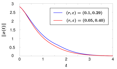
Figure 3. State norm $\|x(t)\|$ of self-triggered control system.

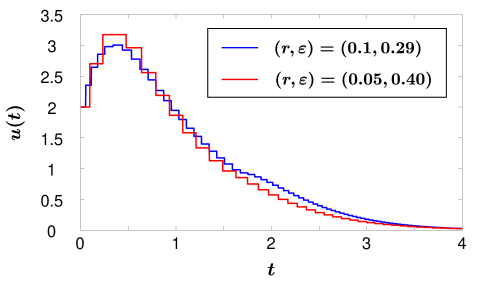
Figure 4. Input $u(t)$ of self-triggered control system.

Figure 5 illustrates inter-event times $t_{k+1}-t_{k}$ in the large perturbation case (blue circle) and the small perturbation case (red squire). The following lower bounds $\theta$ of the minimum inter-event time $\inf_{k\in\mathbb{N}_{0}}(t_{k+1}-t_{k})$ can be computed:

$$\inf_{k\in\mathbb{N}_{0}}(t_{k+1}-t_{k})\geq\theta:=\inf_{\tau\geq 0}\left\{\|F(I-\Delta_{\tau})\|+L\int_{0}^{\tau}\|FT(\tau-s)\|\eta_{L,\varepsilon}(s)ds\geq\varepsilon\right\}.$$

Indeed, using the matrix representations (51), we obtain $\theta=0.0102$ in the large perturbation case and $\theta=0.0147$ in the small perturbation case.

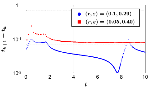
Figure 5. Inter-event times $t_{k+1}-t_{k}$ of self-triggered control system.

As expected from Figure 4, the state is frequently transmitted in the large perturbation case. Moreover, the inter-event times in the large perturbation case take values close to the lower bound $\theta=0.0102$ for $7.6\leq t\leq 7.8$. We see from Figure 5 that the behaviors of inter-event times in the two cases are different. More specifically, inter-event times in the large perturbation case have a periodic nature, and those in the small perturbation case converge. The understanding of the behaviors of inter-event times remains limited even for finite-dimensional linear systems; see, e.g., [28]. Further investigation would be needed to establish the analysis of inter-event times.

3.3. Numerical simulation: Event-triggered control

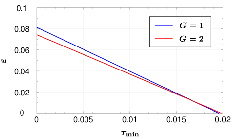
Figure 6. Bound on threshold $\varepsilon$ and lower bound $\tau_{\min}$ of inter-event times of event-triggering mechanism (28).

Next, we provide numerical simulations of the event-triggering mechanism (28). To see the robustness against linear perturbations explained in Remark 2.13, we here do not consider the nonlinear perturbation, that is, we assume that $\psi(x_{2})=x_{2}$ for every $x_{2}\in\mathbb{R}$. Figure 6 shows bounds on the threshold $\varepsilon$ and the lower bound $\tau_{\min}$ of inter-event times obtained from the sufficient condition (45). The blue and red lines depict the bounds in the cases $G=1$ and $G=2$, respectively, where the other parameters of the plant and the controller are set as in (52). In the case $G=2$, we set $\Gamma=2.101$ and $\gamma=1$ for (53). We see from Figure 6 that the difference between the cases $G=1$ and $G=2$ is small and that for example, $(\varepsilon,\tau_{\min})=(0.07,0.001)$ satisfies (45) in both cases. Therefore, the event-triggering mechanism (28) with $(\varepsilon,\tau_{\min})=(0.07,0.001)$ achieves exponential stability for both $G=1$ and $G=2$. In contrast, the sufficient condition (22) does not guarantee that the self-triggering mechanism (20) constructed for $G=1$ achieves exponential stability for any threshold $\varepsilon>0$ in the case $G=2$, since (22) is violated for $L=1$. Note that there is no point in comparing the thresholds $\varepsilon$ between the event-triggering mechanism (28) and the self-triggering mechanism (20). The event-triggering mechanism (28) measures $\|x(t_{k})-x(t)\|$, whereas the self-triggering mechanism (20) estimates $\|Fx(t_{k})-Fx(t)\|$.

Figures 7 and 8 compare the time responses of the event-triggered control system and the periodic sampled-data system in the unperturbed case. We depict the state norm $\|x(t)\|$ in Figure 7 and the input $u(t)$ in Figure 8. The blue and red lines in these figures are for the event-triggered control system and the periodic sampled-data system, respectively. We set the parameters of the plant and the controller as in the previous subsection. The parameters of the event-triggering mechanism (28) are $(\varepsilon,\tau_{\min},\tau_{\max})=(0.07,0.001,0.5)$. The sampling period of the periodic system is $h=0.0205$, which is the numerically obtained maximum value satisfying the sufficient condition (46) for exponential stability. We see from Figure 7 that the state norms of the event-triggered control system and the periodic system look almost identical. In Figure 9, the blue circles and the red squires depict the inter-event times of the event-triggered control system and the periodic system, respectively. We see from Figures 8 and 9 that the number of data transmissions in the even-triggered control system is much smaller than that in the periodic system. This illustrates the effectiveness of event-triggering mechanisms, whose advantage is to change transmission times depending on the state.

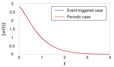
Figure 7. Comparison of state norm $\|x(t)\|$ between event-triggered control system and periodic sampled-data system.

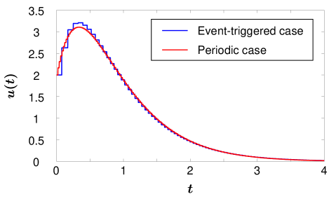
Figure 8. Comparison of input $u(t)$ between event-triggered control system and periodic sampled-data system.

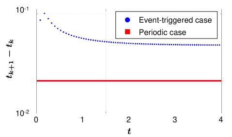
Figure 9. Comparison of inter-event times $t_{k+1}-t_{k}$ between event-triggered control system and periodic sampled-data system.

Finally, we make a comparison of inter-event times between the self-triggering mechanism (20) and the event-triggering mechanism (28). We consider the self-triggering mechanism with $(L,\varepsilon,\tau_{\max})=(\sqrt{5}/20,0.40,0.5)$, which is used for the small perturbation case in the previous subsection, and the event-triggering mechanism with $(\varepsilon,\tau_{\min},\tau_{\max})=(0.07,0.001,0.5)$ as in the simulations for Figures 7–9. As shown above, the lower bounds of inter-event times are $0.0147$ and $0.001$ for the self-triggering mechanism and the event-triggering mechanism, respectively. We see from Figures 5 and 9 that the inter-event times of the self-triggering mechanism are larger than those of the event-triggering mechanism. Hence, the self-triggering mechanism is better with respect to inter-event times than the event-triggering mechanism in this example. The reason is that the self-triggering mechanism estimates the input error $Fx(t)-Fx(t_{k})$, which is more essential for control than the state error $x(t)-x(t_{k})$ used in the event-triggering mechanism.

4. Periodic event-triggering mechanism for unbounded control

In this section, we study event-triggered control for infinite-dimensional systems with unbounded control operators. We consider the evolution equation in the form of (8), but the difference from the bounded control case in Section 2 is that the control operator $B$ is unbounded, i.e., $B\in\mathcal{B}(U,X_{-1})$, where $X_{-1}$ is the extrapolation space of $X$ associated with $T(t)$. In the unbounded control case, we cannot apply standard results on solutions of evolution equations with Lipschitz perturbations developed in Chapter 6 of [27]. Therefore, we need to begin by showing that the integral equation (10) has a unique solution even in the unbounded control case and that this solution satisfies the evolution equation (8) interpreted in $X_{-1}$. To this end, the compactness of the feedback operator plays an important role. Next, we provide the existence result of periodic event-triggering mechanisms that achieve exponential stability. Finally, we turn back to the bounded control case and give a simple sufficient condition for the exponential stability of the periodic event-triggered control system.

4.1. Solution of evolution equation

The following properties of $S_{\tau}$ obtained in Lemma 2.2 of [23] are useful in the analysis of the infinite-dimensional system (8) with an unbounded control operator:

Lemma 4.1 (Lemma 2.2 of [23]).

Let $T(t)$ be a strongly continuous semigroup on $X$ and $B\in\mathcal{B}(U,X_{-1})$, where $X_{-1}$ is the extrapolation space of $X$ associated with $T(t)$. For any $\tau\geq 0$, the operator $S_{\tau}$ defined by

$$S_{\tau}:=\int^{\tau}_{0}T(s)Bds$$

satisfies $S_{\tau}\in\mathcal{B}(U,X)$ and

$$\sup_{0\leq t\leq\tau}\|S_{t}\|_{\mathcal{B}(U,X)}<\infty.$$

Moreover, for every $F\in\mathcal{K}(X,U)$,

$$\lim_{\tau\downarrow 0}\|S_{\tau}F\|_{\mathcal{B}(X)}=0.$$ (54)

Using these properties of $S_{\tau}$, we obtain a result on the existence and regularity of the solution of the integral equation (10).

Theorem 4.2.

Let $\tau_{\min}>0$ and an increasing sequence $\{t_{k}\}_{k\in\mathbb{N}_{0}}$ satisfy $t_{0}=0$ and $t_{k+1}-t_{k}\geq\tau_{\min}$ for every $k\in\mathbb{N}_{0}$. Assume that $A$ is the generator of a strongly continuous semigroup $T(t)$ on $X$, $B\in\mathcal{B}(U,X_{-1})$, $F\in\mathcal{K}(X,U)$, and a nonlinear operator $\phi:X\to X$ satisfies the Lipschitz condition (9). Then the integral equation (10) has a unique solution $x$ in $C(\mathbb{R}_{+},X)$. Furthermore, this solution $x$ satisfies

$$x|_{[t_{k},t_{k+1})}\in C^{1}\big{(}[t_{k},t_{k+1}),X_{-1}\big{)}\qquad\forall k\in\mathbb{N}_{0}$$

and

$$\dot{x}(t)=Ax(t)+BFx(t_{k})+\phi\big{(}x(t)\big{)}\qquad\forall t\in(t_{k},t_{k+1}),~{}\forall k\in\mathbb{N}_{0},$$

which is interpreted in the extrapolation space $X_{-1}$.

By this theorem, we say as in the bounded control case that the solution of the integral equation (10) is called a (mild) solution of the evolution equation (8).

Let $t_{1}>0$ be given. We begin by investigating the integral equation

$$x(t)=T(t)x^{0}+\int^{t}_{0}T(t-s)\Big{(}BFx^{0}+\phi\big{(}x(s)\big{)}\Big{)}ds,~{}~{}t\in[0,t_{1}];\quad x^{0}\in X.$$ (55)

Lemma 4.3.

Assume the same hypotheses on $A,B,F,\phi$ as in Theorem 4.2. Then the integral equation (55) has a unique solution in $C\big{(}[0,t_{1}],X\big{)}$.

Proof.

By Corollary 1.3 on p. 185 in [27], it suffices to show that

$$\zeta(t):=\int^{t}_{0}T(t-s)BFx^{0}ds=S_{t}Fx^{0}$$

satisfies $\zeta\in C\big{(}[0,t_{1}],X\big{)}$.

Let $t\in[0,t_{1})$ and $\tau\in(0,t_{1}-t)$ be given. By the strong continuity of $T(t)$, there exists $c\geq 1$ such that $\|T(t)\|_{\mathcal{B}(X)}\leq c$ for every $t\in[0,t_{1}]$. Since

$$S_{t+\tau}Fx^{0}-S_{t}Fx^{0}=\int^{t+\tau}_{t}T(s)BFx^{0}ds=T(t)\int^{\tau}_{0}T(s)BFx^{0}ds=T(t)S_{\tau}Fx^{0},$$

it follows that

$$\|S_{t+\tau}Fx^{0}-S_{t}Fx^{0}\|\leq c\|S_{\tau}Fx^{0}\|.$$

Lemma 4.1 yields

$$\lim_{\tau\downarrow 0}\|\zeta(t+\tau)-\zeta(t)\|=0,$$

which implies that $\zeta$ is right continuous on $[0,t_{1})$. Similarly, one can show that $\zeta$ is left continuous on $(0,t_{1}]$. Thus, $\zeta\in C\big{(}[0,t_{1}],X\big{)}$. ∎

We next study the differentiability of the solution of the integral equation (55).

Lemma 4.4.

Assume the same hypotheses on $A,B,F,\phi$ as in Theorem 4.2. The solution $x\in C\big{(}[0,t_{1}],X\big{)}$ of the integral equation (55) satisfies

$$x|_{[0,t_{1})}\in C^{1}\big{(}[0,t_{1}),X_{-1}\big{)}$$

and

$$\dot{x}(t)=Ax(t)+BFx(t_{k})+\phi\big{(}x(t)\big{)}\qquad\forall t\in[0,t_{1}),$$

which is interpreted in the extrapolation space $X_{-1}$.

Proof.

Define $g_{1}(t):=BFx^{0}$ and $g_{2}(t):=\phi\big{(}x(t)\big{)}$ for $t\in[0,t_{1})$. By Theorem 2.4 on p. 107 in [27], it is enough to show that for each $i\in\{1,2\}$, $g_{i}\in C\big{(}[0,t_{1}),X_{-1}\big{)}$ and $v_{i}$ defined by

$$v_{i}(t):=\int^{t}_{0}T(t-s)g_{i}(s)ds,\quad t\in[0,t_{1})$$

satisfies $v_{i}\in X$ for every $t\in[0,t_{1})$ and $Av_{i}\in C\big{(}[0,t_{1}),X_{-1}\big{)}$.

Clearly, the constant function $g_{1}$ belongs to $C\big{(}[0,t_{1}),X_{-1}\big{)}$. Since

$$v_{1}(t)=S_{t}Fx^{0},$$

it follows from Lemma 4.1 that $v_{1}(t)\in X$ for every $t\in[0,t_{1})$. Moreover,

$$Av_{1}(t)=(T(t)-I)BFx^{0},$$

and hence $Av_{1}\in C\big{(}[0,t_{1}),X_{-1}\big{)}$ by the strong continuity of $T(t)$.

Let us next investigate $g_{2}$ and $v_{2}$. Since $x\in C\big{(}[0,t_{1}],X\big{)}$ and $\phi$ is Lipschitz continuous on $X$, it follows that $g_{2}\in C\big{(}[0,t_{1}),X\big{)}$. Let $\lambda\in\varrho(A)$ and $(X_{-1},\|\cdot\|_{X_{-1}})$ be the completion of $(X,\|\cdot\|_{-1})$, where $\|x\|_{-1}:=\|(\lambda I-A)^{-1}x\|$ for $x\in X$. Since

$$\|x\|_{X_{-1}}=\|x\|_{-1}\leq\|(\lambda I-A)^{-1}\|_{\mathcal{B}(X)}~{}\!\|x\|\qquad\forall x\in X,$$ (56)

it follows that $g_{2}\in C\big{(}[0,t_{1}),X_{-1}\big{)}$. By definition, $v_{2}(t)\in X$ for every $t\in[0,t_{1})$. To show $Av_{2}\in C\big{(}[0,t_{1}),X_{-1}\big{)}$, it is enough to prove $Ag_{2}\in C\big{(}[0,t_{1}),X_{-1}\big{)}$, because

$$Av_{2}(t)=\int^{t}_{0}T(t-s)Ag_{2}(s)ds;$$

see, e.g., Proposition 1.3.4 on p. 24 in [2] for the continuity property of convolutions.

Since $\lambda I-A$ is an isometry from $X$ to $X_{-1}$ (see, e.g., Theorem II.5.5 on p. 126 in [5]), it follows that for every $t,s\in[0,t_{1})$,

$$\|Ag_{2}(t)-Ag_{2}(s)\|_{X_{-1}} \leq\big{\|}\phi\big{(}x(t)\big{)}-\phi\big{(}x(s)\big{)}\big{\|}+|\lambda|~{}\!\big{\|}\phi\big{(}x(t)\big{)}-\phi\big{(}x(s)\big{)}\big{\|}_{X_{-1}}.$$ (57)

Using $x\in C\big{(}[0,t_{1}],X\big{)}$, the Lipschitz continuity of $\phi$ on $X$, and (56), we obtain $Ag_{2}\in C\big{(}[0,t_{1}),X_{-1}\big{)}$. This completes the proof. ∎

Proof of Theorem 4.2.

Since $x(t_{k})\in X$ for every $k\in\mathbb{N}_{0}$ by Lemma 4.3, we obtain the desired conclusion by repeating the argument in Lemmas 4.3 and 4.4. ∎

4.2. Periodic event-triggering mechanism

We define the increasing sequence $\{t_{k}\}_{k\in\mathbb{N}_{0}}$ by

$$t_{k+1}:=\min\{t_{k}+\ell_{\max}h,~{}\bar{t}_{k+1}\};\quad t_{0}:=0$$ (58a)

$$\bar{t}_{k+1}:=\min\big{\{}\ell h>t_{k}:\|x(\ell h)-x(t_{k})\|>\varepsilon\|x(t_{k})\|,~{}\ell\in\mathbb{N}\big{\}},\quad k\in\mathbb{N}_{0},$$ (58b)

where $h>0$ is a sampling period, $\varepsilon\geq 0$ is a threshold parameter, and $\ell_{\max}\in\mathbb{N}$ determines an upper bound of inter-event times as follows: $t_{k+1}-t_{k}\leq\ell_{\max}h$ for every $k\in\mathbb{N}_{0}$. We call (58) a periodic event-triggering mechanism [10]. In the case $\varepsilon=0$, the state $x(t)$ is transmitted at every $t=kh$, $k\in\mathbb{N}_{0}$, unless $x(kh+h)=x(kh)$. Therefore, the periodic event-triggering mechanism (58) with $\varepsilon=0$ can be regarded as the conventional periodic sampling process. The periodic event-triggering mechanism (58) checks the condition only periodically unlike the event-triggering mechanism (28). This discrete behavior may degrade the control performance for a large $h$, but it makes the periodic event-triggering mechanism (58) better suited for practical implementations.

We analyze the periodic event-triggered control system by discretizing the closed-loop system with period $h$. The resulting discrete-time system has a bounded control operator by Lemma 4.1. Combining this with an estimate of the perturbation term by Gronwall’s inequality, we obtain a sufficient condition for exponential stability.

Lemma 4.5.

Assume that $A$ generates a strongly continuous semigroup $T(t)$ on $X$, $B\in\mathcal{B}(U,X_{-1})$, $F\in\mathcal{K}(X,U)$, and a nonlinear operator $\phi:X\to X$ satisfies the Lipschitz condition (9). Moreover, assume that $\Delta_{h}$ defined by (11) is power stable for some $h>0$, i.e., there exist $\Omega\geq 1$ and $\omega\in(0,1)$ such that

$$\|\Delta_{h}^{k}\|_{\mathcal{B}(X)}\leq\Omega\omega^{k}\qquad\forall k\in\mathbb{N}_{0}.$$

Then the event-triggered control system (8) with the mechanism (58) is exponentially stable for every $\ell_{\max}\in\mathbb{N}$ if $L,\varepsilon\geq 0$ satisfy

$$\varepsilon\Omega\big{(}\|S_{h}F\|_{\mathcal{B}(X)}+c_{3}(e^{c_{2}Lh}-1)\big{)}<1-\omega-c_{1}\Omega(e^{c_{2}Lh}-1),$$ (59)

where

$$c_{1}:=\sup_{0\leq\tau\leq h}\|\Delta_{\tau}\|_{\mathcal{B}(X)},~{}~{}c_{2}:=\sup_{0\leq\tau\leq h}\|T(\tau)\|_{\mathcal{B}(X)},~{}~{}c_{3}:=\sup_{0\leq\tau\leq h}\|S_{\tau}F\|_{\mathcal{B}(X)}.$$ (60)

Proof.

As in the proof of Theorem 5.8 in [36], define a new norm $|\cdot|_{\rm d}$ on $X$ by

$$|x|_{\rm d}:=\sup_{\ell\in\mathbb{N}_{0}}\|\omega^{-\ell}\Delta_{h}^{\ell}x\|,\quad x\in X.$$ (61)

Similarly to the norm $|\cdot|$ defined by (18), the discrete-time counterpart $|\cdot|_{\rm d}$ satisfies

$$\|x\|\leq|x|_{\rm d}\leq\Omega\|x\|,\quad|\Delta_{h}^{k}x|_{\rm d}\leq\omega^{k}|x|_{\rm d}\qquad\forall x\in X,~{}\forall k\in\mathbb{N}_{0}.$$ (62)

For the time sequence $\{t_{k}\}_{k\in\mathbb{N}_{0}}$ defined by (58), let $\ell_{k}\in\mathbb{N}_{0}$ satisfy $t_{k}=\ell_{k}h$. The error $e$ induced by the event-triggering implementation is given by

$$e(\ell h):=x(\ell_{k}h)-x(\ell h),\quad\ell\in[\ell_{k},\ell_{k+1})\cap\mathbb{N}_{0},~{}k\in\mathbb{N}_{0}.$$

Under the periodic event-triggering mechanism (58), the error $e$ satisfies

$$\|e(\ell h)\|\leq\varepsilon\|x(\ell_{k}h)\|\qquad\forall\ell\in[\ell_{k},\ell_{k+1})\cap\mathbb{N}_{0},~{}\forall k\in\mathbb{N}_{0}.$$ (63)

The solution of the integral equation (10) can be rewritten as

$$x(\ell h+\tau)=\Delta_{\tau}x(\ell h)+\int^{\tau}_{0}T(\tau-s)\phi\big{(}x(\ell h+s)\big{)}ds+S_{\tau}Fe(\ell h)$$ (64)

for every $\tau\in(0,h]$ and $\ell\in\mathbb{N}_{0}$. Gronwall’s inequality yields

$$\|x(\ell h+\tau)\| \leq\big{(}c_{1}\|x(\ell h)\|+\varepsilon c_{3}\|x(\ell_{k}h)\|\big{)}+c_{2}L\int^{\tau}_{0}\|x(\ell h+s)\|ds$$

$$\leq e^{c_{2}L\tau}\big{(}c_{1}\|x(\ell h)\|+\varepsilon c_{3}\|x(\ell_{k}h)\|\big{)}$$ (65)

for every $\tau\in(0,h]$, $\ell\in[\ell_{k},\ell_{k+1})\cap\mathbb{N}_{0}$, and $k\in\mathbb{N}_{0}$, where $c_{1},c_{2},c_{3}\geq 0$ are defined by (60). It follows from (64) with $\tau=h$ that

$$\big{|}x\big{(}(\ell+1)h\big{)}\big{|}_{\rm d} \leq\omega|x(\ell h)|_{\rm d}+\varepsilon\Omega\|S_{h}F\|_{\mathcal{B}(X)}|x(\ell_{k}h)|_{\rm d}$$

$$\qquad+c_{2}L\Omega\int^{h}_{0}e^{c_{2}Ls}ds\big{(}c_{1}|x(\ell h)|_{\rm d}+\varepsilon c_{3}|x(\ell_{k}h)|_{\rm d}\big{)}$$

$$\leq\widetilde{\omega}_{1}(L)|x(\ell h)|_{\rm d}+\delta_{1}(L,\varepsilon)|x(\ell_{k}h)|_{\rm d},$$ (66)

where

$$\widetilde{\omega}_{1}(L):=\omega+c_{1}\Omega(e^{c_{2}Lh}-1),\quad\delta_{1}(L,\varepsilon):=\varepsilon\Omega\big{(}\|S_{h}F\|_{\mathcal{B}(X)}+c_{3}(e^{c_{2}Lh}-1)\big{)}.$$

Proceeding by induction, we have

$$\big{|}x(\ell_{k+1}h)\big{|}_{\rm d} \leq\widetilde{\omega}_{1}(L)^{p_{k}}|x(\ell_{k}h)|_{\rm d}+\frac{1-\widetilde{\omega}_{1}(L)^{p_{k}}}{1-\widetilde{\omega}_{1}(L)}\delta_{1}(L,\varepsilon)|x(\ell_{k}h)|_{\rm d}$$

$$=\big{(}\widetilde{\omega}_{1}(L)^{p_{k}}[1-\delta_{2}(L,\varepsilon)]+\delta_{2}(L,\varepsilon)\big{)}|x(\ell_{k}h)|_{\rm d}\qquad\forall k\in\mathbb{N}_{0},$$

where

$$p_{k}:=\ell_{k+1}-\ell_{k},\quad\delta_{2}(L,\varepsilon):=\frac{\delta_{1}(L,\varepsilon)}{1-\widetilde{\omega}_{1}(L)}.$$

For $L,\varepsilon\geq 0$, (59) holds if and only if $\widetilde{\omega}_{1}(L)<1$ and $\delta_{2}(L,\varepsilon)<1$. Let $L,\varepsilon\geq 0$ satisfy (59), and define $\widetilde{\omega}:=\widetilde{\omega}_{1}(L)$ and $\delta:=\delta_{2}(L,\varepsilon)$. If we define the function $f_{\rm p}$ on $\mathbb{N}$ by

$$f_{\rm p}(\ell):=\frac{-\log(\widetilde{\omega}^{\ell}(1-\delta)+\delta)}{\ell h},$$

then $f_{\rm p}$ is positive and monotonically decreasing on $\mathbb{N}$. Therefore,

$$\big{|}x(\ell_{k+1}h)\big{|}_{\rm d}\leq e^{-\gamma_{0}p_{k}h}|x(\ell_{k}h)|_{\rm d}\qquad\forall k\in\mathbb{N}_{0},$$

where $\gamma_{0}:=f_{\rm p}(\ell_{\max})>0$. By induction, we obtain

$$|x(\ell_{k}h)|_{\rm d}\leq e^{-\gamma_{0}\ell_{k}h}|x^{0}|_{\rm d}\qquad\forall x^{0}\in X,~{}\forall k\in\mathbb{N}_{0}.$$

Using (65) and (66) again, we obtain

$$\|x(\ell_{k}h+\tau)\| \leq Me^{-\gamma_{0}\ell_{k}h}\|x^{0}\|$$

$$\leq(Me^{\gamma_{0}\ell_{\max}h})e^{-\gamma_{0}(\ell_{k}h+\tau)}\|x^{0}\|\qquad\forall\tau\in[0,p_{k}h],~{}\forall k\in\mathbb{N}_{0}$$

for some $M>0$. Thus, the event-triggered control system is exponentially stable. ∎

Define an operator $A_{BF}$ on $X$ by

$$A_{BF}x:=(A+BF)x\quad\text{with~{}~{}}\mathop{\rm dom}\nolimits(A_{BF}):=\{x\in X:(A+BF)x\in X\},$$ (67)

which we distinguish from the unbounded operator $A+BF$ on $X_{-1}$ with $\mathop{\rm dom}\nolimits(A+BF)=X$. Under the assumption that $T(t)$ is analytic, Theorem 4.8 in [23] shows that the exponential stability of linear periodic sampled-data systems is robust with respect to sampling.

Theorem 4.6 (Theorem 4.8 in [23]).

Assume that $A$ generates an analytic semigroup $T(t)$ on $X$, $B\in\mathcal{B}(U,X_{-1})$, and $F\in\mathcal{K}(X,U)$. Moreover, assume that the semigroup generated by $A_{BF}$ given in (67) is exponentially stable. Then there exists $h^{*}>0$ such that for every $h\in(0,h^{*})$, the linear periodic sampled-data system (8) with $\phi\equiv 0$ and $t_{k+1}-t_{k}\equiv h$ is exponentially stable.

See also [31] for another result on robustness of stabilization with respect to sampling in the unbounded control case.

Combining Lemma 4.5 and Theorem 4.6, we obtain a result on the existence of a periodic event-triggering mechanism that achieves exponential stability.

Theorem 4.7.

Assume the same hypotheses on $A,B,F,T(t)$ as in Theorem 4.6, and choose $h>0$ so that the linear periodic sampled-data system (8) with $\phi\equiv 0$ and $t_{k+1}-t_{k}\equiv h$ is exponentially stable. Moreover, assume that a nonlinear operator $\phi:X\to X$ satisfies the Lipschitz condition (9). Then there exist $\varepsilon^{*}=\varepsilon^{*}(h)>0$ and $L^{*}=L^{*}(h)>0$ such that for every $\varepsilon\in[0,\varepsilon^{*}]$ and every $L\in[0,L^{*}]$, the system (8) with the periodic event-triggering mechanism (58) is exponentially stable.

Proof.

By Lemma 2.3 in [23], the linear periodic sampled-data system (8) with $\phi\equiv 0$ and $t_{k+1}-t_{k}\equiv h$ is exponentially stable if and only if the operator $\Delta_{h}$ is power stable. Combining this with Lemma 4.5, we obtain the desired result. ∎

Finally, we return to the bounded control case $B\in\mathcal{B}(U,X)$. Suppose that the semigroup $T_{BF}(t)$ is exponentially stable, i.e, (14) holds for some $\Gamma\geq 1$ and $\gamma>0$. For $h>0$, define

$$W(h):=\Gamma e^{\gamma h}\sup_{0\leq t\leq h}\big{\|}T(h-t)BF[I-T_{BF}(t)]\big{\|}_{\mathcal{B}(X)}.$$ (68)

As explained in Remark 2.14, $\Delta_{h}$ defined by (11) is power stable if $W(h)<\gamma$. In such a case, we obtain

$$\|\Delta_{h}^{k}\|_{\mathcal{B}(X)}\leq\Gamma\omega^{k}\qquad\forall k\in\mathbb{N}_{0},$$

where $\omega:=1-[\gamma-W(h)]e^{-\gamma h}h$; see (3.6) in the proof of Theorem 3.1 of [23]. This fact, together with Lemma 4.5, yields a simple sufficient condition for the periodic event-triggered control system to be exponentially stable. To avoid the trivial case in which the open-loop system is exponentially stable, we here additionally assume that $S_{h}F\not=0$ holds for every $h>0$ satisfying $W(h)<\gamma$.

Corollary 4.8.

Suppose that Assumption 2.4 is satisfied and $S_{h}F\not=0$ holds for every $h>0$ satisfying $W(h)<\gamma$. The system (8) with the periodic event-triggering mechanism (58) is exponentially stable for every $\ell_{\max}\in\mathbb{N}$ if $h>0$ and $L,\varepsilon\geq 0$ satisfy

$$\varepsilon<\frac{[\gamma-W(h)]e^{-\gamma h}h-c_{1}\Gamma(e^{c_{2}Lh}-1)}{\Gamma\big{(}\|S_{h}F\|_{\mathcal{B}(X)}+c_{3}(e^{c_{2}Lh}-1)\big{)}},$$ (69)

where $c_{1},c_{2},c_{3}\geq 0$ are defined by (60).

For the numerical example of the unperturbed case $\psi(x_{2})=x_{2}$ in Section 3, one can observe that the bounds of the parameters $(\varepsilon,h)$ satisfying (69) are similar to to those of $(\varepsilon,\tau_{\min})$ shown in Figure 6. Moreover, as expected easily, if $h$ is small, then numerical simulations of the periodic event-triggered control systems are also closely similar to those in Figures 7–9. We omit these figures because they show almost identical trends as Figures 6–9.

5. Conclusion

In this paper, we have analyzed the exponential stability of infinite-dimensional event/self-triggered control systems with Lipschitz perturbations. The fundamental assumption is that the feedback operator is compact, which guarantees the strict positiveness of inter-event times and the existence of the mild solution of the evolution equation with an unbounded control operator. We have shown that if the parameters of the event/self-triggering mechanisms are appropriately chosen, then exponential stability is preserved under all perturbations with sufficiently small Lipschitz constants. Moreover, in the bounded control case, we have provided simple sufficient conditions for exponential stability.

Received xxxx 20xx; revised xxxx 20xx.

References

• [1] A. Anta and P. Tabuada, To sample or not to sample: Self-triggered control for nonlinear systems, IEEE Trans. Automat. Control, 55 (2010), 2030–2042.
• [2] W. Arendt, C. J. K. Batty, M. Hieber and F. Neubrander, Vector-valued Laplace Transforms and Cauchy Problems, Basel: Birkhäuser, 2001.
• [3] L. Baudouin, S. Marx and S. Tarbouriech, Event-triggered damping of a linear wave equation, Proc. CPDE-CEPS’19 (2019) 58–63.
• [4] R. F. Curtain and H. J. Zwart, An Introduction to Infinite-Dimensional Linear Systems Theory, New York: Springer, 1995.
• [5] K.-J. Engel and R. Nagel, One-Parameter Semigroups for Linear Evolution Equations, New York: Springer, 2000.
• [6] N. Espitia, A. Girard, N. Marchand and C. Prieur, Event-based control of linear hyperbolic systems of conservation laws, Automatica, 70 (2016), 275–287.
• [7] N. Espitia, A. Girard, N. Marchand and C. Prieur, Event-based boundary control of a linear $2\times 2$ hyperbolic system via backstepping approach, IEEE Trans. Automat. Control, 63 (2018), 2686–2693.
• [8] L. Etienne, S. Di Gennaro and J.-P. Barbot, Periodic event-triggered observation and control for nonlinear Lipschitz systems using impulsive observers, Int. J. Robust Nonlinear Control, 27 (2017), 4363–4380.
• [9] R. Goebel, R. Sanfelice and A. Teel, Hybrid dynamical systems, IEEE Control Syst. Mag., 29 (2009), 28–93.
• [10] W. P. M. H. Heemels, M. C. F. Donkers and A. R. Teel, Periodic event-triggered control for linear systems, IEEE Trans. Automat. Control, 58 (2013), 847–861.
• [11] W. P. M. H. Heemels, J. Sandee and P. van den Bosch, Analysis of event-driven controllers for linear systems, Int. J. Control, 81 (2008), 571–590.
• [12] A. Ilchmann, Z. Ke and H. Logemann, Indirect sampled-data control with sampling period adaptation, Int. J. Control, 84 (2011), 424–431.
• [13] Z. Jiang, B. Cui, W. Wu and B. Zhuang, Event-driven observer-based control for distributed parameter systems using mobile sensor and actuator, Comput. Math. Appl., 72 (2016), 2854–2864.
• [14] W. Kang and E. Fridman, Distributed sampled-data control of Kuramoto-Sivashinsky equation, Automatica, 95 (2018), 514–524.
• [15] I. Karafyllis and M. Krstic, Sampled-data boundary feedback control of 1-D parabolic PDEs, Automatica, 87 (2018), 226–237.
• [16] I. Karafyllis, M. Krstic and K. Chrysafi, Adaptive boundary control of constant-parameter reaction-diffusion PDEs using regulation-triggered finite-time identification, Automatica, 103 (2019), 166–179.
• [17] Z. Ke, H. Logemann and R. Rebarber, Approximate tracking and disturbance rejection for stable infinite-dimensional systems using sampled-data low-gain control, SIAM J. Control Optim., 48 (2009), 641–671.
• [18] Z. Ke, H. Logemann and R. Rebarber, A sampled-data servomechanism for stable well-posed systems, IEEE Trans. Automat. Control, 54 (2009), 1123–1128.
• [19] Z. Ke, H. Logemann and S. Townley, Adaptive sampled-data integral control of stable infinite-dimensional linear systems, Systems Control Lett., 58 (2009), 233–240.
• [20] D. Lehmann and J. Lunze, Event-based control with communication delays and packet losses, Int. J. Control, 85 (2012), 563–577.
• [21] P. Lin, H. Liu and G. Wang, Output feedback stabilization for heat equations with sampled-data controls, J. Differential Equ., 268 (2020), 5823–5854.
• [22] H. Logemann, Stabilization of well-posed infinite-dimensional systems by dynamic sampled-data feedback, SIAM J. Control Optim., 51 (2013), 1203–1231.
• [23] H. Logemann, R. Rebarber and S. Townley, Stability of infinite-dimensional sampled-data systems, Trans. Amer. Math. Soc., 355 (2003), 3301–3328.
• [24] H. Logemann, R. Rebarber and S. Townley, Generalized sampled-data stabilization of well-posed linear infinite-dimensional systems, SIAM J. Control Optim., 44 (2005), 1345–1369.
• [25] H. Logemann and S. Townley, Discrete-time low-gain control of uncertain infinite-dimensional systems, IEEE Trans. Automat. Control, 42 (1997), 22–37.
• [26] A. Mironchenko and C. Prieur, Input-to-state stability of infinite-dimensional systems: recent results and open questions, SIAM Review, 62 (2020), 529–614.
• [27] A. Pazy, Semigroups of Linear Operators and Applications to Partial Differential Equations, New York: Springer, 1983.
• [28] R. Postoyan, R. G. Sanfelice and W. P. M. H. Heemels, Inter-event times analysis for planar linear event-triggered controlled systems, Proc. 58th IEEE CDC (2019), 1662–1667.
• [29] R. Rebarber and S. Townley, Generalized sampled data feedback control of distributed parameter systems, Systems Control Lett., 34 (1998), 229–240.
• [30] R. Rebarber and S. Townley, Nonrobustness of closed-loop stability for infinite-dimensional systems under sample and hold, IEEE Trans. Automat. Control, 47 (2002), 1381–1385.
• [31] R. Rebarber and S. Townley, Robustness with respect to sampling for stabilization of Riesz spectral systems, IEEE Trans. Automat. Control, 51 (2006), 1519–1522.
• [32] A. Selivanov and E. Fridman, Distributed event-triggered control of diffusion semilinear PDEs, Automatica, 68 (2016), 344–351.
• [33] P. Tabuada, Event-triggered real-time scheduling of stabilizing control tasks, IEEE Trans. Automat. Control, 52 (2007), 1680–1685.
• [34] T. J. Tarn, J. R. Zavgern and X. Zeng, Stabilization of infinite-dimensional systems with periodic gains and sampled output, Automatica, 24 (1988), 95–99.
• [35] M. Tucsnak and G. Weiss, Observation and Control of Operator Semigroups, Basel: Birkhäuser, 2009.
• [36] M. Wakaiki and H. Sano, Event-triggered control of infinite-dimensional systems, SIAM J. Control Optim., 58 (2020), 605–635.
• [37] M. Wakaiki and H. Sano, Sampled-data output regulation of unstable well-posed infinite-dimensional systems with constant reference and disturbance signals, Math. Control Signals Systems, 32 (2020), 43–100.
• [38] M. Wakaiki and Y. Yamamoto, Stability analysis of perturbed infinite-dimensional sampled-data systems, Systems Control Lett., 138 (2020), 1–8, Article 104652.
• [39] X. Wang and M. D. Lemmon, Self-triggered feedback control systems with finite-gain $\mathcal{L}_{2}$ stability, IEEE Trans. Automat. Control, 54 (2009), 452–467.