A shape theorem for a one-dimensional growing particle system with a bounded number of occupants per site

Abstract

We consider a one-dimensional discrete-space birth process with a bounded number of particle per site. Under the assumptions of the finite range of interaction, translation invariance, and non-degeneracy, we prove a shape theorem. We also derive a limiting estimate and an exponential estimate on the fluctuations of the position of the rightmost particle.

Mathematics subject classification: 60K35, 82C22.

1 Introduction

In this paper we consider a one-dimensional growing particle system with a finite range of interaction. A configuration is specified by assigning to each site $x\in\mathbb{Z}$ a number of particles ${\eta(x)\in\{0,1,...,N\}}$, $n\in\mathbb{N}$, occupying $x$. The state space of the process is thus $\{0,1,...,N\}^{\mathbb{Z}}$. Under additional assumptions such as non-degeneracy and translation invariance, we show that the system spreads linearly in time and the speed can be expressed as an average value of a certain functional over a certain measure. A respective shape theorem and a fluctuation result are given.

The first shape theorem was proven in [Ric73] for a discrete-space growth model. A general shape theorem for discrete-space attractive growth models can be found in [Dur88, Chapter 11]. In the continuous-space settings shape results for growth models have been obtained in [Dei03] for a model of growing sets, and in [BDPK⁺17] for a continuous-space particle birth process.

The asymptotic behavior of the position of the rightmost particle of the branching random walk under various assumptions is given in [Dur83], [Gan00], and [Dur79], see also references therein. A sharp condition for a shape theorem for a random walk with restriction is given in [BDPKT]. The speed of propagation for a one-dimensional discrete-space supercritical branching random walk with an exponential moment condition can be found in [Big95]. More refined limiting properties have been obtained recently, such as the limiting law of the minimum or the limiting process seen from its tip, see [Aïd13, ABBS13, ABK13, ABR09]. Blondel [Blo13] proves a shape result for the East model, which is a non-attractive particle system.

In many cases the underlying stochastic model is attractive, which enables the application of a subadditive ergodic theorem. Typically shape results have been obtained using the subadditivity property in one form or another. This is not only the case for the systems of motionless particles listed above (see, among others, [Dur88, Dei03, BDPK⁺17]) but also for those with moving particles, see e.g. shape theorem for the frog model [AMP02]. A certain kind of subadditivity was also used in [KS08], where a shape theorem for a non-attractive model involving two types of moving particles is given. In the present paper our model is not attractive and we do not rely on subadditivity (see also Remark 2.6). We work with motionless particles.

In addition to the shape theorem, we also provide a sub-Gaussian limit estimate on the deviation of the position of the rightmost particle from the mean. Various sub-exponential and -Gaussian estimates on the convergence rate for the first passage percolation under different assumptions can be found in e.g. [Kes93, Ahl19]. We also derive an exponential non-asymptotic bound valid for all times.

On Page 2 we describe a particular model with the birth rate declining in crowded locations. This is achieved by augmenting the free branching rate with certain multipliers describing the effects of the competition on the parent’s ability to procreate and offspring’s ability to survive in a dense location. This process is in general non-attractive.

The paper is organized as follows. In Section 2 we describe our model in detail, give our assumptions, and formulate the main results. In Section 3 we outline the construction of the process as a unique solution to a stochastic equation driven by a Poisson point process. We note here that this very much resembles the construction via graphical representation. In Section 4 we prove the main results, Theorems 2.4, 2.7, and 2.8. Some numerical simulations are discussed in Section 5.

2 Model and the main results

We consider here a one dimensional continuous-time discrete-space birth process with multiple particles per site allowed. The state space of our process is $\mathcal{X}:=\{0,1,...,N\}^{\mathbb{Z}}$. For $\eta\in\mathcal{X}$ and $x\in\mathbb{Z}$, $\eta(x)$ is interpreted as the number of particles, or individuals, at $x$.

The evolution of the process can be described as follows. If the system is in the state $\eta\in\mathcal{X}$, a single particle is added at $x\in\mathbb{Z}$ (that is, the $\eta(x)$ is increased by $1$) at rate $b(x,\eta)$ provided that $\eta(x)<N$; the number of particles at $x$ does not grow anymore once it reaches $N$. Here $b:\mathbb{Z}\times\mathcal{X}\to\mathbb{R}_{+}$ is the map called a ‘birth rate’. The heuristic generator of the model is given by

$$LF(\eta)=\sum\limits_{x\in\mathbb{Z}}b(x,\eta)[F(\eta^{+x})-F(\eta)],$$ (1)

where $\eta^{+x}(y)=\eta(y)$, $y\neq x$, and

$$\eta^{+x}(x)=\begin{cases}\eta(x)+1,&\text{ if }\eta(x)<N,\\ \eta(x),&\text{ if }\eta(x)=N.\end{cases}$$ (2)

We make the following assumptions about $b$. For $y\in\mathbb{Z}$, $\eta\in\mathcal{X}$, let $\eta\odot y\in\mathcal{X}$ be the shift of $\eta$ by $y$, so that $[\eta\odot y](x)=\eta(x-y)$.

Condition 2.1 (Translation invariance).

For any $x,y\in\mathcal{X}$ and $\eta\in\mathcal{X}$,

$$b(x+y,\eta\odot y)=b(x,\eta).$$

Condition 2.2 (Finite range of interaction).

For some $R\in\mathbb{N}$,

$$b(x,\eta)=b(x,\xi),\ \ \ \ x\in\mathbb{Z},\ \eta,\xi\in\mathcal{X}$$ (3)

whenever $\eta(z)=\xi(z)$ for all $z\in\mathbb{Z}$ with $|x-z|\leq R$.

Put differently, Condition 2.2 means that interaction in the model has a finite range $R$. Since the number of particles occupying a given site cannot grow larger than $N$, with no loss in generality we can also assume that

$$b(x,\eta)=0,\ \ \ \ \text{if }\eta(x)=N.$$ (4)

For $\eta\in\mathcal{X}$ we define the set of occupied sites

$$\text{occ}(\eta)=\{z\in\mathbb{Z}:\eta(z)>0\}.$$

Condition 2.3 (non-degeneracy).

For every $x\in\mathbb{Z}$ and $\eta\in\mathcal{X}$, $b(x,\eta)>0$ if and only if there exists $y\in\text{occ}(\eta)$ with $|x-y|\leq R$.

Note that by translation invariance, $\sup\limits_{x\in\mathbb{Z},\eta\in\mathcal{X}}b(x,\eta)$ is finite because this supremum is equal to

$$\overline{\mathbf{b}}:=\max\{b(0,\eta)\mid\eta\in\mathcal{X},\eta(y)=0\text{ for all }y\text{ with }|y|>R\}.$$ (5)

Similarly, it follows from translation invariance and non-degeneracy that

$$\underline{\mathbf{b}}:=\inf\limits_{\begin{subarray}{c}x\in\mathbb{Z},\eta\in\mathcal{X},\\ dist(x,\text{occ}(\eta))\leq R\end{subarray}}b(x,\eta)>0.$$ (6)

The construction of the birth process is outlined in Section 3. Let $(\eta_{t})_{t\geq 0}=(\eta_{t})$ be the birth process with birth rate $b$ and initial condition $\eta_{0}(k)=\mathds{1}\{k=0\}$, $k\in\mathbb{Z}$. For an interval $[a,b]\subset\mathbb{R}$ and $c>0$, $c[a,b]$ denotes the interval $[ca,cb].$ The following theorem characterizes the growth of the set of occupied sites.

Theorem 2.4.

There exists $\lambda_{r},\lambda_{l}>0$ such that for every $\varepsilon>0$ a.s. for sufficiently large $t$,

$$\bigg{(}(1-\varepsilon)[-\lambda_{l}t,\lambda_{r}t]\cap\mathbb{Z}\bigg{)}\subset\textnormal{occ}(\eta_{t})\subset(1+\varepsilon)[-\lambda_{l}t,\lambda_{r}t].$$ (7)

Remark 2.5.

If we assume additionally that the birth rate is symmetric, that is, if for all $x\in\mathbb{Z}$, $\eta\in\mathcal{X}$,

$$b(x,\eta)=b(-x,\tilde{\eta}),$$

where $\tilde{\eta}(y)=\eta(-y)$, then, as can be seen from the proof, $\lambda_{l}=\lambda_{r}$ holds true in Theorem 2.4.

Remark 2.6.

Note that under our assumptions the following attractiveness property does not have to hold: if for two initial configuration $\eta^{1}_{0}\leq\eta^{2}_{0}$, then $\eta^{1}_{t}\leq\eta^{2}_{t}$ for all $t\geq 0$. This renders inapplicable the techniques based on a subadditive ergodic theorem (e.g. [Lig85]) which are usually used in the proof of shape theorems (see e.g. [Dur88, Dei03, BDPK⁺17]). On the other hand, our technique relies heavily on the dimension being one as the analysis is based on viewing the process from its tip. It would be of interest to extend the result to dimensions $\mathrm{d}\geq 2$. To the best of our knowledge, even for the following modification of Eden’s model, the shape theorem has not been proven. Take $\mathrm{d}=2$, $N=1$ (only one particle per site is allowed), and for $x\in\mathbb{Z}^{2}$ and $\eta\subset\mathbb{Z}^{2}$ with $\eta(x)=0$ let

$$b(x,\eta)=\mathds{1}\left\{\sum\limits_{y\in\mathbb{Z}^{2}:|y-x|=1}\eta(y)\in\{1,2\}\right\}.$$

and define $\xi_{t}=\eta_{t}\cup\{y\in\mathbb{Z}^{2}:y\text{ is surrounded by particles of }\eta_{t}\}$, $t\geq 0$. It is reasonable to expect the shape theorem to hold for $\xi_{t}$. Note that the classical Eden model can be seen as a birth process with rate

$$b(x,\eta)=\mathds{1}\left\{\sum\limits_{y\in\mathbb{Z}^{2}:|y-x|=1}\eta(y)>0\right\}$$

started from a single particle at the origin.

For $\eta\in\mathcal{X}$ with $\sum\limits_{x\in\mathbb{Z}}\eta(x)<\infty$, let

$$\text{tip}(\eta):=\max\{m\in\mathbb{Z}:\eta(m)>0\}$$

be the position of the rightmost occupied site. Let

$$X_{t}=\text{tip}(\eta_{t}).$$ (8)

By Theorem 2.4 a.s.

$$\frac{X_{t}}{t}\to\lambda_{r},\ \ \ t\to\infty.$$ (9)

We now give two results on the deviations of $X_{t}$ from the mean. The first theorem gives a sub-Gaussian limiting estimate on the fluctuations around the mean, while the second provices an exponential estimate for all $t\geq 0$. Let $\lambda_{r}$ be as in (9).

Theorem 2.7.

There exist $\mathrm{C}_{1},\sigma>0$ such that

$$\limsup\limits_{t\to\infty}\mathbb{P}\left\{|X_{t}-\lambda_{r}t|\geq q\sqrt{t}\right\}\leq\mathrm{C}_{1}e^{-q^{2}\sigma^{2}},\ \ \ q>0.$$ (10)

Theorem 2.8.

There exist $\mathrm{C}_{2},\theta>0$ such that

$$\mathbb{P}\left\{|\frac{X_{t}}{t}-\lambda_{r}|\geq q\right\}\leq\mathrm{C}_{2}e^{-\theta qt},\ \ \ q>0,\ t>0.$$ (11)

Of course, Theorems 2.7 and 2.8 also apply to the position of the leftmost occupied site provided that $\lambda_{r}$ is replaced with $\lambda_{l}$.

Birth rate with regulation via fecundity and establishment. As an example of a non-trivial model satisfying our assumptions, consider the birth process in $\mathcal{X}$ with birth rate

$$\begin{multlined}b(x,\eta)=\exp\left\{-\sum\limits_{u\in\mathbb{Z}}\phi(u-x)\eta(u)\right\}\sum\limits_{y\in\mathbb{Z}}\left[a(x-y)\eta(y)\exp\left\{-\sum\limits_{v\in\mathbb{Z}}\psi(v-y)\eta(v)\right\}\right],\\ x\in\mathbb{Z},\eta\in\mathcal{X},\eta(x)<N.\end{multlined}b(x,\eta)=\exp\left\{-\sum\limits_{u\in\mathbb{Z}}\phi(u-x)\eta(u)\right\}\sum\limits_{y\in\mathbb{Z}}\left[a(x-y)\eta(y)\exp\left\{-\sum\limits_{v\in\mathbb{Z}}\psi(v-y)\eta(v)\right\}\right],\\ x\in\mathbb{Z},\eta\in\mathcal{X},\eta(x)<N.$$ (12)

where $a,\phi,\psi:\mathbb{Z}\to\mathbb{R}_{+}$ have a finite range, $\sum\limits_{x\in\mathbb{Z}}a(x)>0$. The birth rate (12) is a modification of the free branching rate

$$\begin{multlined}b(x,\eta)=\sum\limits_{y\in\mathbb{Z}}a(x-y)\eta(y),\ \ \ x\in\mathbb{Z},\eta\in\mathcal{X},\eta(x)<N.\end{multlined}b(x,\eta)=\sum\limits_{y\in\mathbb{Z}}a(x-y)\eta(y),\ \ \ x\in\mathbb{Z},\eta\in\mathcal{X},\eta(x)<N.$$

The purpose of the modification is to include damping mechanisms reducing the birth rate in the dense regions. The first exponent multiplier in (12), $\exp\left\{-\sum\limits_{u\in\mathbb{Z}}\phi(u-x)\eta(u)\right\}$, represents the reduction in establishment at location $x$ if $\eta$ has many individuals around $x$. The second exponent multiplier, $\exp\left\{-\sum\limits_{v\in\mathbb{Z}}\psi(v-y)\eta(v)\right\}$, represents diminishing fecundity of an individual at $y$ surrounded by many other individuals. Further description and motivation for an equivalent continuous-space model can be found in [FKK13, BDF⁺]. We note here that the birth process with birth rate (12) does not in general possess the attractiveness property mentioned in Remark 2.6. Some numerical observations on this model are collected in Section 5.

3 Construction of the process

Similarly to [Gar95], [GK06], [BDPK⁺17], we construct the process as a solution to the stochastic equation

$$\eta_{t}(k)=\int\limits_{(0,t]\times\{k\}\times[0,\infty)}\mathds{1}_{[0,b(i,\eta_{s-})]}(u)P(ds,di,du)+\eta_{0}(k),\quad t\geq q,\ k\in\mathbb{Z},$$ (13)

where $(\eta_{t})_{t\geq 0}$ is a càdlàg $\mathcal{X}$-valued solution process, $P$ is a Poisson point process on $\mathbb{R}_{+}\times\mathbb{Z}\times\mathbb{R}_{+}$, the mean measure of $P$ is $ds\times\#\times du$ ($\#$ is the counting measure on $\mathbb{Z}$ ). We require the processes $P$ and $\eta_{0}$ to be independent of each other. Equation (13) is understood in the sense that the equality holds a.s. for every $k\in\mathbb{Z}$ and $t\geq 0$. In the integral on the right-hand side of (13), $i=k$ is the location and $s$ is the time of birth of a new particle. Thus, the integral from $0$ to $t$ represents the number of births at $k\in\mathbb{Z}$ which occurred before $t$.

This section follows closely Section 5 in [BDPK⁺17]. Note that the only difference to Theorem 5.1 from [BDPK⁺17] is that the ‘geographic’ space is discrete ($\mathbb{Z}$) rather than continuous ($\mathbb{R}^{\mathrm{d}}$ as in [BDPK⁺17]). This change requires no new arguments, ideas, or techniques in comparison to [BDPK⁺17].

We will make the following assumption on the initial condition:

$$\mathbb{E}\sum\limits_{i\in\mathbb{Z}}\eta_{0}(i)<\infty.$$ (14)

Let $P$ be defined on a probability space $(\Omega,\mathscr{F},\mathbb{P})$. We say that the process $P$ is compatible with an increasing, right-continuous and complete filtration of $\sigma$-algebras $(\mathscr{F}_{t},t\geq 0)$, $\mathscr{F}_{t}\subset\mathscr{F}$, if $P$ is adapted, that is, all random variables of the type $P(\bar{T}_{1}\times U)$, $\bar{T}_{1}\in\mathscr{B}([0;t])$, $U\in\mathscr{B}(\mathbb{Z}\times\mathbb{R}_{+})$, are $\mathscr{F}_{t}$-measurable, and all random variables of the type $P((t,t+h]\times U)$, $h\geq 0$, $U\in\mathscr{B}(\mathbb{Z}\times\mathbb{R}_{+})$, are independent of $\mathscr{F}_{t}$ (here we consider the Borel $\sigma$-algebra for $\mathbb{Z}$ to be the collection $2^{\mathbb{Z}}$ of all subsets of $\mathbb{Z}$).

We equip $\mathcal{X}$ with the product set topology and $\sigma$-algebra generated by the open sets in this topology.

Definition 3.1.

A (weak) solution of equation (13) is a triple $((\eta_{t})_{t\geq 0},P)$, $(\Omega,\mathscr{F},\mathbb{P})$, $(\{\mathscr{F}_{t}\}_{t\geq 0})$, where

(i) $(\Omega,\mathscr{F},\mathbb{P})$ is a probability space, and $\{\mathscr{F}_{t}\}_{t\geq 0}$ is an increasing, right-continuous and complete filtration of sub-$\sigma$-algebras of $\mathscr{F}$,

(ii) $P$ is a Poisson point process on $\mathbb{R}_{+}\times\mathbb{Z}\times\mathbb{R}_{+}$ with intensity $ds\times\#\times du$,

(iii) $\eta_{0}$ is a random $\mathscr{F}_{0}$-measurable element in $\mathcal{X}$ satisfying (14),

(iv) the processes $P$ and $\eta_{0}$ are independent, $P$ is compatible with $\{\mathscr{F}_{t}\}_{t\geq 0}$,

(v) $(\eta_{t})_{t\geq 0}$ is a càdlàg $\mathcal{X}$-valued process adapted to $\{\mathscr{F}_{t}\}_{t\geq 0}$, $\eta_{t}\big{|}_{t=0}=\eta_{0}$,

(vi) all integrals in (13) are well-defined,

$$\mathbb{E}\int\limits_{0}^{t}ds\sum\limits_{i\in\mathbb{Z}}b(i,\eta_{s-})<\infty,\ \ \ t>0,$$

(vii) equality (13) holds a.s. for all $t\in[0,\infty]$ and all $k\in\mathbb{Z}$.

Let

$$\mathscr{S}^{0}_{t}=\sigma\bigl{\{} \eta_{0},P([0,q]\times\{k\}\times C),$$ (15)

$$q\in[0,t],k\in\mathbb{Z},C\in\mathscr{B}(\mathbb{R}_{+})\bigr{\}},$$

and let $\mathscr{S}_{t}$ be the completion of $\mathscr{S}^{0}_{t}$ under $P$. Note that $\{\mathscr{S}_{t}\}_{t\geq 0}$ is a right-continuous filtration.

Definition 3.2.

A solution of (13) is called strong if $(\eta_{t})_{t\geq 0}$ is adapted to $(\mathscr{S}_{t},t\geq 0)$.

Definition 3.3.

We say that pathwise uniqueness holds for (13) if for any two (weak) solutions $((\eta_{t})_{t\geq 0},P)$, $(\Omega,\mathscr{F},\mathbb{P})$, $(\{\mathscr{F}_{t}\}_{t\geq 0})$ and $((\eta_{t}^{\prime})_{t\geq 0},P)$, $(\Omega,\mathscr{F},\mathbb{P})$, $(\{\mathscr{F}_{t}\}_{t\geq 0})$ with $\eta_{0}=\eta_{0}^{\prime}$ we have

$$\mathbb{P}\left\{\eta_{t}=\eta_{t}^{\prime}\text{ for all }t\geq 0\right\}=1.$$ (16)

Definition 3.4.

We say that joint uniqueness in law holds for equation (13) with an initial distribution $\nu$ if any two (weak) solutions $((\eta_{t}),P)$ and $((\eta_{t}^{\prime}),P^{\prime})$ of (13), $Law(\eta_{0})=Law(\eta_{0}^{\prime})=\nu$, have the same joint distribution:

$$Law((\eta_{t}),P)=Law((\eta_{t}^{\prime}),P^{\prime}).$$

Theorem 3.5.

Pathwise uniqueness, strong existence and joint uniqueness in law hold for equation (13). The unique solution is a Markov process with respect to the filtration $(\mathscr{S}_{t},t\geq 0)$.

The proof follows exactly the proof of Theorem 5.1 in [BDPK⁺17] and is therefore omitted. We also note here that the unique solution of (13) satisfies a.s. $\eta_{t}(x)\leq N$ for $x\in\mathbb{Z}$ and $t\geq 0$ by (4).

4 Proofs

Let $\mathbb{Z}_{+}=\mathbb{N}\cup\{0\}$, $\mathbb{Z}_{-}=-\mathbb{Z}_{+}$, and $\beta_{t}:\mathbb{Z}_{-}\to\mathbb{Z}_{+}$ be $\eta_{t}$ seen from its tip defined by

$$\beta_{t}(-n)=\eta_{t}(\text{tip}(\eta_{t})-n),\ \ \ n=0,1,2,...$$

Let $h_{t}$ be the position of first block of $R$ sites occupied by $N$ particles seen from the tip,

$$h_{t}:=\max\{m\in\mathbb{Z}_{-}:\beta_{t}(m-1)=\beta_{t}(m-2)=...=\beta_{t}(m-R)=N\}\vee\min\{m\in\mathbb{Z}_{-}:\beta_{t}(m)>0\}.$$

We adopt here the convention $\max\{\varnothing\}=-\infty$, so that if there are no blocks of $R$ consecutive sites occupied by $N$ particles, $h_{t}$ equals to the furthest from the origin occupied site for $\beta_{t}$. Finally, define $\alpha_{t}:\mathbb{Z}_{-}\to\{0,1,...,N\}$ by

$$\alpha_{t}(m)=\beta_{t}(m)\mathbf{I}\{m\geq h_{t}\}.$$

Thus, $\alpha_{t}$ can be interpreted as the part of $\eta_{t}$ seen from its tip until the first block of $R$ sites occupied by $N$ particles. The process $(\alpha_{t},t\geq 0)$ takes values in a countable space

$$\Upsilon:=\left\{\gamma\middle|\gamma:\mathbb{Z}_{-}\to\{0,1,...,N\},\sum\limits_{x\in\mathbb{Z}_{-}}\gamma(x)<\infty\right\}.$$

Let us underline that $\alpha_{t}$ is a function of $\eta_{t}$; we denote by $\mathcal{A}$ the respective mapping $\mathcal{A}:\mathcal{X}\to\Upsilon$, so that $\alpha_{t}=\mathcal{A}(\eta_{t})$.

Lemma 4.1.

The process $(\alpha_{t},t\geq 0)$ is a continuous-time positive recurrent Markov process with a countable state space. Furthermore, $(\alpha_{t},t\geq 0)$ is strongly ergodic.

Proof. We start from a key observation: for $t\geq 0$, conditionally on the event

$$\eta(m)=\eta(m+1)=...=\eta(m+R)=N$$

for some $m\in\mathbb{Z}$, the families $\{\eta_{s}(y),s\geq t,y<m\}$ and $\{\eta_{s}(y),s\geq t,y>m+R\}$ are independent. Consequently, $(\alpha_{t},t\geq 0)$ is an irreducible continuous-time Markov chain. The definitions and properties of continuous-time Markov chains used here can be found e.g. in [Che04, Section 4.4]. Translation invariance Condition 2.1 ensures that $(\alpha_{t},t\geq 0)$ is time-homogeneous. Define $\mathbf{0}_{\Upsilon}\in\Upsilon$ by $\mathbf{0}_{\Upsilon}(m)=0$, $m=0,-1,-2,...$ Now, let us note that

$$\inf\limits_{\gamma\in\Upsilon}\mathbb{P}\left[\alpha_{t+1}=\mathbf{0}_{\Upsilon}\middle|\alpha_{t}=\gamma\right]=\inf\limits_{\gamma\in\Upsilon}\mathbb{P}\left[\alpha_{1}=\mathbf{0}_{\Upsilon}\middle|\alpha_{0}=\gamma\right]>0.$$ (17)

Indeed, for $\eta_{0}$ such that $\mathcal{A}(\eta_{0})=\alpha_{0}=\gamma$,

$$\mathbb{P}\left\{\alpha_{1}=\mathbf{0}_{\Upsilon}\right\}\geq\mathbb{P}\left\{\text{tip}(\eta_{1})=\text{tip}(\eta_{0})\right\}$$

$$\times\mathbb{P}\left\{\eta_{1}(\text{tip}(\eta_{1}))=\eta_{1}(\text{tip}(\eta_{1}-1))=...=\eta_{1}(\text{tip}(\eta_{1})-R+1)=N\right\}>0,$$

and the last expression is separated from $0$ uniformly in $\gamma$. It follows from (17) that the state $\mathbf{0}_{\Upsilon}$ is positive recurrent. Since $(\alpha_{t},t\geq 0)$ is irreducible, it follows that it is also positive recurrent. The strong ergodicity follows from (17). ∎

Denote by $\pi$ the ergodic measure for $(\alpha_{t},t\geq 0)$. For $\gamma\in\Upsilon$, let $\eta^{\gamma}\in\mathcal{X}$ be

$$\eta^{\gamma}(m)=\begin{cases}\gamma(m),&\ \ \ m\leq 0\\ 0,&\ \ \ m>0\end{cases}$$ (18)

Note that $\mathcal{A}(\eta^{\gamma})=\gamma$. Define $f:\Upsilon\to\mathbb{R}_{+}$ by

$$f(\gamma)=\sum\limits_{m=1}^{N}mb(x,\eta^{\gamma}).$$

Note that

$$\sup\limits_{\gamma\in\Upsilon}f(\gamma)\leq\frac{R(R+1)}{2}\overline{\mathbf{b}}.$$ (19)

Since $f$ is bounded, by the ergodic theorem for continuous-time Markov chains a.s.

$$\frac{1}{t}\int\limits_{0}^{t}f(\alpha_{s})ds\to\langle f\rangle_{\pi},$$ (20)

where $\langle f\rangle_{\pi}:=\sum\limits_{\gamma\in\Upsilon}\pi(\gamma)f(\gamma)$ (here for convenience $\pi(\{\gamma\})$ is denoted by $\pi(\gamma)$, $\gamma\in\Upsilon$).

Recall that $X_{t}=\text{tip}(\eta_{t})$. The process $(X_{t},t\geq 0)$ is an increasing pure jump type Markov process, and the rate of jump of size $m\in\{1,2,...,R\}$ at time $t$ is $b(X_{t}+m,\eta_{t})$. Indeed, note that

$$\begin{split}X_{t}&=\sum\limits_{k=1}^{R}k\int\limits_{(0,t]\times\mathbb{Z}\times[0,\infty)}\mathds{1}\{i=k+X_{s-}\}\mathds{1}_{[0,b(k+X_{s-},\eta_{s-})]}(u)P(ds,di,du)\\ &=\sum\limits_{k=1}^{R}k\int\limits_{(0,t]\times[0,\infty)}\mathds{1}_{[0,b(k+X_{s-},\eta_{s-})]}(u)P^{(k)}(ds,du),\end{split}$$ (21)

where the integrator is defined by

$$\begin{multlined}P^{(k)}(A\times B)=P\big{(}\{(t,i,u)\in\mathbb{R}_{+}\times\mathbb{Z}\times\mathbb{R}_{+}\big{|}X_{t-}+k=i,(t,u)\in A\times B\}\big{)},\\ \ \ A,B\in\mathscr{B}(\mathbb{R}_{+}),\ \ k\in\{1,...,m\}.\end{multlined}P^{(k)}(A\times B)=P\big{(}\{(t,i,u)\in\mathbb{R}_{+}\times\mathbb{Z}\times\mathbb{R}_{+}\big{|}X_{t-}+k=i,(t,u)\in A\times B\}\big{)},\\ \ \ A,B\in\mathscr{B}(\mathbb{R}_{+}),\ \ k\in\{1,...,m\}.$$

In other words, $P^{(k)}(A\times B)$ is $P(A\times\{i\}\times B)$ if $A\subset\{t:X_{t-}+k=i\}$ and $B\in\mathscr{B}(\mathbb{R}_{+})$. Note that $P^{(k)}$ is a Poisson point process on $\mathbb{R}_{+}\times\mathbb{R}_{+}$ with mean measure $ds\times du$ (this follows for example from the strong Markov property of a Poisson point process, as formulated in the appendix in [BDPK⁺17], applied to the jump times of $(X_{t},t\geq 0)$ ). The indicators in (21) are

$$\begin{aligned} &\mathds{1}\{i=k+X_{s-}\}=\begin{cases}1,&\text{ if }i=k+X_{s-},\\ 0,&\text{ otherwise },\\ \end{cases}\\ \end{aligned} \begin{aligned} &\mathds{1}_{[0,b(k+X_{t},\eta_{s-})]}(u)=\begin{cases}1,&\text{ if }u\in[0,b(k+X_{t},\eta_{s-})],\\ 0,&\text{ otherwise }.\\ \end{cases}\\ \end{aligned}$$

Therefore, by e.g. (3.8) in Section 3, Chapter 2 of [IW89], the process

$$M_{t}:=X_{t}-\int\limits_{0}^{t}\sum\limits_{k=1}^{R}kb(X_{t}+k,\eta_{s})ds=X_{t}-\int\limits_{0}^{t}f(\alpha_{s})ds.$$ (22)

is a martingale with respect to the filtration $(\mathscr{S}_{t},t\geq 0)$ defined below (15).

We now formulate a strong law of large numbers for martingales. The following theorem is an abridged version of [HH80, Theorem 2.18].

Theorem 4.2.

Let $\{S_{n}=\sum\limits_{i=1}^{n}x_{i},n\in\mathbb{N}\}$ be an $\{\mathscr{S}_{n}\}$-martingale and $\{U_{n}\}_{n\in\mathbb{N}}$ be a non-decreasing sequence of positive real numbers, $\lim\limits_{n\to\infty}U_{n}=\infty$. Then for $p\in[1,2]$ we have

$$\lim\limits_{n\to\infty}U_{n}^{-1}S_{n}=0$$

a.s. on the set $\left\{\sum\limits_{i=1}^{\infty}U_{n}^{-p}\mathbb{E}\big{\{}|x_{i}|^{p}\big{|}\mathscr{F}_{i-1}\big{\}}<\infty\right\}$.

Lemma 4.3.

Strong law of large numbers applies to $(M_{t},t\geq 0)$:

$$\mathbb{P}\left\{\frac{M_{t}}{t}\to 0\right\}=1.$$ (23)

Proof. Let $\Delta M_{n}=M_{n+1}-M_{n}$. Then $\Delta M_{n}$ is stochastically dominated by $\mathrm{V}_{1}+2\mathrm{V}_{2}+...+R\mathrm{V}_{R}+\frac{R(R+1)}{2}\overline{\mathbf{b}}$, where $\mathrm{V}_{1},...,\mathrm{V}_{R}$ are independent Poisson random variables with mean $\overline{\mathbf{b}}$, independent of $\mathscr{F}_{n}$. Applying the strong law of large numbers for martingales from Theorem 4.2 with $p=\frac{3}{2}$ and $U_{n}=n$, we get a.s.

$$\frac{1}{n}\sum\limits\Delta M_{n}\to 0.$$ (24)

Since a.s. for every $\varepsilon>0$,

$$\mathbb{P}\left\{\sup\limits_{s\in[0,1]}|M_{n+s}-M_{s}|\geq\varepsilon n\text{ for infinitely many }n\right\}=0,$$

(23) follows. ∎

Proof of Theorem 2.4. Let $\lambda_{r}=\langle f\rangle_{\pi}$. From (20) and Lemma 4.3 we get a.s.

$$\frac{1}{t}X_{t}-\langle f\rangle_{\pi}\to 0,$$ (25)

or

$$\frac{1}{t}\text{tip}(\eta_{t})-\lambda_{r}\to 0.$$ (26)

In the same way (due to the symmetric nature of our assumptions) we can show the equivalent of (26) for the leftmost occupied site $Y_{t}$ for $\eta_{t}$: there exists $\lambda_{l}>0$ such that for any $\varepsilon>0$ a.s. for large $t$,

$$\frac{|Y_{t}|}{t}-\lambda_{l}\to 0.$$ (27)

Hence the second inclusion in (7) holds. (As an aside we point out here that $\lambda_{l}$ can be expressed as an average value in the same way as $\lambda_{r}=\langle f\rangle_{\pi}$. To do so, we would need to define the opposite direction counterparts to $(\beta_{t},t\geq 0)$, $(\alpha_{t},t\geq 0)$, $f$, and other related objects.)

To show the first inclusion in (7), we fix $\varepsilon>0$, and for each $x\in\mathbb{Z}$. By (26) and (27), a.s. for large $t$

$$\left[-\lambda_{l}t\left(1+\frac{\varepsilon}{4}\right)^{-1},\lambda_{r}t\left(1+\frac{\varepsilon}{4}\right)^{-1}\right]\subset[Y_{t},X_{t}].$$ (28)

For $x\in\mathbb{Z}$, let

$$\begin{split}\sigma(x)&:=\inf\{t\geq 0:dist(x,\text{occ}(\eta_{t}))\leq R\},\\ \tau(x)&:=\inf\{t\geq 0:\eta_{t}(x)\geq 1\}=\inf\{t\geq 0:x\in\text{occ}(\eta_{t})\}.\end{split}$$ (29)

Clearly, for any $x\in\mathbb{Z}$, $0\leq\sigma(x)\leq\tau(x)$. Because of the finite range assumption, by (28) a.s. for $x\in\mathbb{N}$ with large $|x|$

$$\sigma(x)\leq\frac{(1+\frac{\varepsilon}{4})|x|}{\lambda_{r}}.$$ (30)

By (6), the random variable $\tau(x)-\sigma(x)$ is stochastically dominated by an exponential random variable with mean $\underline{\mathbf{b}}^{-1}$. In particular

$$\mathbb{P}\left\{\tau(x)-\sigma(x)\geq\frac{\varepsilon|x|}{4\lambda_{r}}\right\}\leq\exp\{-\frac{\varepsilon|x|\underline{\mathbf{b}}}{4\lambda_{r}}\}.$$

Since $\sum\limits_{x\in\mathbb{N}}\exp\{-\frac{\varepsilon|x|\underline{\mathbf{b}}}{4\lambda_{r}}\}<\infty$, a.s. for all but finitely many $x\in\mathbb{N}$ we have

$$\tau(x)-\sigma(x)\leq\frac{\varepsilon|x|}{4\lambda_{r}}.$$

Hence from (30) a.s. for all but finitely many $x\in\mathbb{N}$,

$$\tau(x)\leq\frac{(1+\frac{\varepsilon}{2})|x|}{\lambda_{r}}.$$ (31)

From (31) it follows that a.s. if $t$ is large and $x\in\mathbb{N}$, $|x|\leq\frac{\lambda_{r}t}{1+\frac{\varepsilon}{2}}$, then $\tau(x)\leq t$. Note that $\text{occ}(\eta_{t})=\{x\in\mathbb{Z}:\tau(x)\leq t\}$. Thus for large $t$.

$$\left[0,\frac{\lambda_{r}t}{1+\frac{\varepsilon}{2}}\right]\cap\mathbb{Z}\subset\text{occ}(\eta_{t}).$$ (32)

Repeating this argument verbatim for $-x\in\mathbb{N}$ and $\lambda_{l}$ in place of $x\in\mathbb{N}$ and $\lambda_{r}$ respectively, we find that

$$\left[-\frac{\lambda_{l}t}{1+\frac{\varepsilon}{2}},0\right]\cap\mathbb{Z}\subset\text{occ}(\eta_{t}).$$ (33)

Since $1-\varepsilon\leq\frac{1}{1+\frac{\varepsilon}{2}}$ for $\varepsilon>0$, the first inclusion in (7) follows from (32) and (33). ∎

Lemma 4.4.

For some $\varrho^{2}\in(0,+\infty)$ a.s.

$$\frac{1}{t}[M]_{t}\to\varrho^{2},\ \ \ t\to\infty.$$ (34)

Proof. Let $\theta_{0}=0$ and denote by $\theta_{n}$, $n\in\mathbb{N}$, the moment of $n$-th hitting of $\mathbf{0}_{\Upsilon}$ by the Markov chain $(\alpha_{t},t\geq 0)$. For $n\in\mathbb{N}$, define a random piecewise constant function $Z_{n}$ by

$$Z_{n}(t)=\alpha_{(t+\theta_{n})\wedge\theta_{n+1}},\ \ \ t\geq 0.$$ (35)

The sequence $\{Z_{n}\}_{n\in\mathbb{N}}$ can be seen as a sequence of independent random elements in the Skorokhod space $\mathcal{D}:=D([0,\infty),\Upsilon)$ endowed with the usual Skorokhod topology.

Let $G:\mathcal{D}\to\mathbb{Z}_{+}$ be the functional such that $G(Z_{n})=[M]_{\theta_{n+1}-\theta_{n}}$ is the change of $([M]_{t})$ between $\theta_{n}$ and $\theta_{n+1}$. The function $G$ can be written down explicitly, but it is not necessary for our purposes. Now, since the number of jumps for $Z_{1}$ has exponential tails, for any $m\in\mathbb{N}$

$$\mathbb{E}\left\{G^{m}(Z_{1})\right\}<\infty.$$ (36)

By the strong law of large numbers, a.s.

$$\frac{1}{n}\sum\limits_{i=1}^{n}G(Z_{i})\to\mathbb{E}\left\{G(Z_{1})\right\}>0.$$ (37)

Since $\theta_{2}-\theta_{1}$, $\theta_{3}-\theta_{2}$, …, are i.i.d. random variables, a.s.

$$\frac{\theta_{n}}{n}\to\mathbb{E}\left\{\theta_{2}-\theta_{1}\right\}>0.$$ (38)

For $t>0$, let $n=n(t)\in\mathbb{N}$ be such that $t\in[\theta_{n},\theta_{n+1})$. Then by (37) and (38) a.s.

$$\lim\limits_{t\to\infty}\frac{[M]_{t}}{t}=\lim\limits_{t\to\infty}\frac{[M]_{\theta_{1}}+\sum\limits_{i=1}^{n(t)}G(Z_{i})}{t}=\lim\limits_{t\to\infty}\frac{\sum\limits_{i=1}^{n(t)}G(Z_{i})}{n(t)}\frac{n(t)}{t}=\frac{\mathbb{E}\left\{G(Z_{1})\right\}}{\mathbb{E}\left\{\theta_{2}-\theta_{1}\right\}}>0.$$ (39)

∎

Before proceeding with the final part of the paper, we formulate a central limit theorem for martingales used in the proof of Theorem 2.7. The statement below is a corollary of [Hel82, Theorem 5.1].

Proposition 4.5.

Assume that (34) holds and that for some $K>0$ a.s.

$$\sup\limits_{t\geq 0}|M_{t}-M_{t-}|\leq K.$$

Then

$$\frac{1}{\sqrt{t}}M_{t}\overset{d}{\to}\mathcal{N}(0,\varrho^{2}),\ \ \ t\to\infty.$$ (40)

Proposition 4.5 follows from [Hel82, Theorem 5.1, (b)] by taking $M_{n}$ in notation of [Hel82] to be $\frac{M_{tn}}{n}$ in our notation.

Proof of Theorem 2.7. By Lemma 4.1, the continuous-time Markov chain $(\alpha_{t},t\geq 0)$ is strongly ergodic. Since the function $f$ is bounded, the central limit theorem holds for $(\alpha_{t},t\geq 0)$ by [LZ15, Theorem 3.1]. That is, the convergence in distribution takes place

$$\frac{1}{\sqrt{t}}\left[\int\limits_{0}^{t}f(\alpha_{s})ds-\langle f\rangle_{\pi}\right]\overset{d}{\to}\mathcal{N}(0,\sigma^{2}_{f}),\ \ \ t\to\infty,$$ (41)

where $\sigma^{2}_{f}\geq 0$ is a constant depending on $f$, and $\mathcal{N}(c,\sigma^{2})$ is the normal distribution with mean $c\in\mathbb{R}$ and variance $\sigma^{2}\geq 0$. Recall that $\langle f\rangle_{\pi}=\lambda_{r}$. By (41), for some $C_{1},\sigma_{1}>0$

$$\limsup\limits_{t\to\infty}\mathbb{P}\left\{\left|\int\limits_{0}^{t}f(\alpha_{s})ds-\lambda_{r}t\right|\geq q\sqrt{t}\right\}\leq C_{1}e^{-q^{2}\sigma_{1}^{2}},\ \ \ q>0.$$ (42)

Recall that $M_{t}$ was defined in (22). By Lemma 4.4 for some $\varrho^{2}\in(0,+\infty)$ a.s.

$$\frac{1}{t}[M]_{t}\to\varrho^{2},\ \ \ t\to\infty.$$ (43)

By the martingale central limit theorem (Proposition 4.5)

$$\frac{1}{\sqrt{t}}M_{t}\overset{d}{\to}\mathcal{N}(0,\varrho^{2}),\ \ \ t\to\infty.$$ (44)

Hence for some $C_{2},\sigma_{2}>0$

$$\limsup\limits_{t\to\infty}\mathbb{P}\left\{\left|X_{t}-\int\limits_{0}^{t}f(\alpha_{s})ds\right|\geq q\sqrt{t}\right\}\leq C_{2}e^{-q^{2}\sigma_{2}^{2}},\ \ \ q>0.$$ (45)

By (42) and (45),

$$\limsup\limits_{t\to\infty}\mathbb{P}\left\{\left|X_{t}-\lambda_{r}t\right|\geq q\sqrt{t}\right\}\leq C_{3}e^{-q^{2}\sigma_{3}^{2}},\ \ \ q>0,$$ (46)

for some $C_{3},\sigma_{3}>0$. ∎

Proof of Theorem 2.8. By (21), (22), and [IW89, (3.9), Page 62, Section 3, Chapter 2], the predictable quadratic variation

$$\langle M\rangle_{t}=\langle X\rangle_{t}=\int\limits_{0}^{t}\sum\limits_{k=1}^{R}k^{2}b(k+X_{s-},\eta_{s-})ds=\int\limits_{0}^{t}g(\alpha_{s-})ds,$$ (47)

where $g:\Upsilon\to\mathbb{R}_{+}$ is such that $g(\alpha)=\sum\limits_{k=1}^{R}k^{2}b(k+\text{tip}(\eta),\eta)$ whenever $\mathcal{A}(\eta)=\alpha$. Recall that the mapping $\mathcal{A}$ was defined on Page 4; $g(\alpha)$ does not depend on the choice of $\eta\in\mathcal{A}^{-1}(\alpha)$.

By [CG08, Theorem 1.1] (see also [Wu00, Theorem 1 and Remark 3a])

$$\mathbb{P}\left\{\left|\frac{1}{t}\int\limits_{0}^{t}g(\alpha_{s-})ds-\langle g\rangle_{\pi}\right|\geq q\right\}\leq C_{1}e^{-\delta_{q}t},\ \ \ q>0,t\geq 0,$$ (48)

where $C_{1}>0$, $\delta_{q}>0$ depends on $q$ but not on $t$, and $\delta_{q}$ grows not slower than linearly as a function of $q$. Note that the jumps of $(M_{t},t\geq 0)$ do not exceed $R$. By an exponential inequality for martingales with bounded jumps, [vdG95, Lemma 2.1], for any $a,b>0$

$$\mathbb{P}\left\{|M_{t}|\geq a,\langle M\rangle_{t}\leq b\text{ for some }t\geq 0\right\}\leq\exp\left\{-\frac{a^{2}}{2(aR+b)}\right\}.$$ (49)

Taking here $a=rt$, $b=\langle g\rangle_{\pi}(1+\varepsilon)t$ for $r>0$, $\varepsilon\in(0,1)$, we get for $t\geq 0$

$$\mathbb{P}\left\{|M_{t}|\geq rt,\langle M\rangle_{t}\leq\langle g\rangle_{\pi}(1+\varepsilon)t\right\}\leq\exp\left\{-\frac{r^{2}}{2(rR+\langle g\rangle_{\pi}(1+\varepsilon))}t\right\}.$$ (50)

By (47) and (48),

$$\mathbb{P}\left\{\langle M\rangle_{t}>\langle g\rangle_{\pi}(1+\varepsilon)t\right\}\leq\mathbb{P}\left\{\frac{1}{t}|\langle M\rangle_{t}-\langle g\rangle_{\pi}|\geq\varepsilon\langle g\rangle_{\pi}\right\}\leq C_{1}e^{-\delta_{\varepsilon\langle g\rangle_{\pi}}t}.$$ (51)

By (50) and (51) we get

$$\begin{gathered}\mathbb{P}\left\{|M_{t}|\geq rt\right\}\leq\mathbb{P}\left\{|M_{t}|\geq rt,\langle M\rangle_{t}\leq\langle g\rangle_{\pi}(1+\varepsilon)t\right\}+\mathbb{P}\left\{\langle M\rangle_{t}>\langle g\rangle_{\pi}(1+\varepsilon)t\right\}\\ \leq\exp\left\{-\frac{r^{2}}{2(rR+\langle g\rangle_{\pi}(1+\varepsilon))}t\right\}+Ce^{-\delta_{\varepsilon\langle g\rangle_{\pi}}t}\leq Ce^{-\delta_{1}rt},\ \ \ t\geq 0,\end{gathered}$$ (52)

where $\delta_{1}>0$ does not depend on $r$ or $t$.

Recalling the definition of $M$ in (22), we rewrite (52) as

$$\mathbb{P}\left\{\left|X_{t}-\int\limits_{0}^{t}f(\alpha_{s})ds\right|\geq r\right\}\leq C_{2}e^{-\delta_{2}rt},\ \ \ t\geq 0,$$ (53)

where $C_{2},\delta_{2}>0$. By [CG08, Theorem 1.1] (or [Wu00, Theorem 1, Remark 3a]),

$$\mathbb{P}\left\{\left|\frac{1}{t}\int\limits_{0}^{t}f(\alpha_{s-})ds-\langle f\rangle_{\pi}\right|\geq r\right\}\leq C_{3}e^{-\delta_{3}rt},\ \ \ t\geq 0,$$ (54)

where the constant $\delta_{3}$ does not depend on $r$. Combining (53) and (54) yields (11) and completes the proof. ∎

Remark 4.6.

We see from the proofs that the non-degeneracy condition can be weakened. In particular, (6) can be removed if we instead require $(\alpha_{t},t\geq 0)$ to be strongly ergodic with the ergodic measure satisfying $\langle f\rangle_{\pi}>0$. Of course, $\text{occ}(\eta)$ in Theorem 2.4 would need to be replaced with the set of sites surrounded by $\text{occ}(\eta)$. Some changes in the proof would have to be made. In particular, if $\pi(\mathbf{0}_{\Upsilon})=0$, the moments of time $\theta_{n}$ in the proof of Lemma 4.4 would need to be redefined as the hitting moments of a state $\gamma\in\Upsilon$ with $\pi(\gamma)>0$.

Remark 4.7.

It would be of interest to see if the finite range condition can be weakened to include interactions decaying exponentially or polynomially fast with the distance. If the interaction range is infinite, there is no reason for $(\alpha_{t},t\geq 0)$ to be a recurrent Markov chain, let alone a strongly ergodic one. It may be the case however that the process seen from the tip $(\beta_{t},t\geq 0)$ turns out to possess some kind of a mixing property, which would enable application of limit theorems.

5 Numerical simulations and monotonicity of the speed

We start this section with the following conjecture claiming that the speed is a monotone functional of the birth rate. Consider two birth processes $(\eta^{(1)}_{t},t\geq 0)$ and $(\eta^{(2)}_{t},t\geq 0)$ with different birth rates $b_{1}$ and $b_{2}$, respectively, satisfying conditions of Theorem 2.4. Denote by $\lambda_{r}^{(j)}$ the speed at which $(\eta^{(j)}_{t},t\geq 0)$ is spreading to the right in the sense of Theorem 2.4, $j=1,2$.

Question 5.1.

Assume that for all $x\in\mathbb{Z}$ and $\eta\in\mathcal{X}$

$$b_{1}(x,\eta)\leq b_{2}(x,\eta).$$ (55)

Is it always true that $\lambda_{r}^{(1)}\leq\lambda_{r}^{(2)}$?

The answer to Question 5.1 is positive if $b_{2}$ is additionally assumed to be monotone in the second argument, that is, if

$$b_{2}(x,\eta)\leq b_{2}(x,\zeta),\ \ \ x\in\mathbb{Z}$$

whenever $\eta\leq\zeta$. Indeed, in this case the two birth processes $(\eta^{(1)}_{t},t\geq 0)$ and $(\eta^{(2)}_{t},t\geq 0)$ with rates $b_{1}$ and $b_{2}$ are coupled in such a way that a.s.

$$\eta^{(1)}_{t}\leq\eta^{(2)}_{t},\ \ \ t\geq 0$$

(see Lemma 5.1 in [BDPK⁺17]). One might think that the answer is positive in a general case, too.

It turns out that the birth rate with fecundity and establishment regulation discussed on Page 2 links up naturally with Question 5.1. Let the birth rate $b$ be as in (12) with $R=N=3$, $a(x)=\mathds{1}\{|x|\leq 3\}$,

$$\psi(x)=c_{\text{fec}}\left[\mathds{1}\{|x|=0\}+\frac{1}{2}\mathds{1}\{|x|=1\}\right],\ \ \ \psi(x)=c_{\text{est}}\left[\mathds{1}\{|x|=0\}+\frac{1}{2}\mathds{1}\{|x|=1\}\right].$$

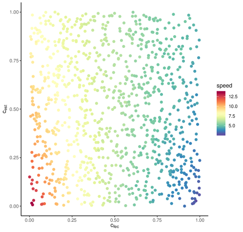
Figure 1: The speed of the tip for various $c_{\text{fec}},c_{\text{est}}$. For each pair, the speed is computed as the average speed of the tip $X_{t}$ between $t_{1}=100$ and $t_{2}=1000$, that is, as $\frac{X_{t_{2}}-X_{t_{1}}}{t_{2}-t_{1}}$. Early evolution is excluded to reduce bias.

Note that $b$ decreases as either of the parameters $c_{\text{fec}}$ and $c_{\text{est}}$ increases. Figure 1 shows the speed of the model with birth rate (12) for a thousand randomly chosen from $[0,1]^{2}$ pairs of parameters $(c_{\text{fec}},c_{\text{est}})$.

Interestingly, we observe that for the values of $c_{\text{fec}}$ close to one, the speed increases as a function of $c_{\text{est}}$. This phenomenon is more apparent on Figure 2, where the speed is computed as a function of $c_{\text{est}}$ with $c_{\text{fec}}=1$. This example demonstrates that the answer to Question 5.1 is negative without additional assumptions on $b_{1}$ and $b_{2}$.

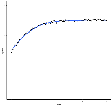
Figure 2: The speed as a function of $c_{\text{est}}$. The other parameter with is fixed $c_{\text{fec}}=1$. Each estimate is computed as $\frac{X_{t_{2}}-X_{t_{1}}}{t_{2}-t_{1}}$ with $t_{1}=100$ and $t_{2}=10000$.

On Figure 3 ten different trajectories with $c_{\text{fec}}=c_{\text{est}}=0.5$ are shown. Numerical analysis was conducted in R [R C19] and figures were produced using the package ggplot2 [Wic09].

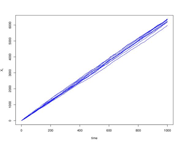
Figure 3: Ten trajectories of the tip. The parameters are $c_{\text{fec}}=c_{\text{est}}=0.5$.

References

- [ABBS13] Elie Aïdékon, Julien Berestycki, Éric Brunet, and Zhan Shi. Branching brownian motion seen from its tip. Probability Theory and Related Fields, 157(1-2):405–451, 2013.
- [ABK13] Louis-Pierre Arguin, Anton Bovier, and Nicola Kistler. The extremal process of branching brownian motion. Probability Theory and related fields, 157(3-4):535–574, 2013.
- [ABR09] Louigi Addario-Berry and Bruce Reed. Minima in branching random walks. Ann. Probab., 37(3):1044–1079, 2009.
- [Ahl19] Daniel Ahlberg. A temporal perspective on the rate of convergence in first-passage percolation under a moment condition. Braz. J. Probab. Stat., 33(2):397–401, 2019.
- [Aïd13] Elie Aïdékon. Convergence in law of the minimum of a branching random walk. The Annals of Probability, 41(3A):1362–1426, 2013.
- [AMP02] O. S. M. Alves, F. P. Machado, and S. Yu. Popov. The shape theorem for the frog model. Ann. Appl. Probab., 12(2):533–546, 2002.
- [BDF+] Viktor Bezborodov, Luca Di Persio, Dmitri Finkelshtein, Yuri Kondratiev, and Oleksandr Kutoviy. Fecundity regulation in a spatial birth-and-death process. Stoch. Dyn. To appear.
- [BDPK+17] V. Bezborodov, L. Di Persio, T. Krueger, M. Lebid, and T. Ożański. Asymptotic shape and the speed of propagation of continuous-time continuous-space birth processes. Advances in Applied Probability, 50(1):74–101, 2017.
- [BDPKT] V. Bezborodov, L. Di Persio, T. Krueger, and P. Tkachov. Spatial growth processes with long range dispersion: microscopics, mesoscopics, and discrepancy in spread rate. Ann. Appl. Probab. To appear.
- [Big95] J. D. Biggins. The growth and spread of the general branching random walk. Ann. Appl. Probab., 5(4):1008–1024, 1995.
- [Blo13] O. Blondel. Front progression in the East model. Stochastic Process. Appl., 123(9):3430–3465, 2013.
- [CG08] Patrick Cattiaux and Arnaud Guillin. Deviation bounds for additive functionals of Markov processes. ESAIM Probab. Stat., 12:12–29, 2008.
- [Che04] Mu-Fa Chen. From Markov chains to non-equilibrium particle systems. World Scientific Publishing Co., Inc., River Edge, NJ, second edition, 2004.
- [Dei03] M. Deijfen. Asymptotic shape in a continuum growth model. Adv. in Appl. Probab., 35(2):303–318, 2003.
- [Dur79] Richard Durrett. Maxima of branching random walks vs. independent random walks. Stochastic Processes and their Applications, 9(2):117–135, 1979.
- [Dur83] R. Durrett. Maxima of branching random walks. Z. Wahrsch. Verw. Gebiete, 62(2):165–170, 1983.
- [Dur88] Richard Durrett. Lecture notes on particle systems and percolation. The Wadsworth & Brooks/Cole Statistics/Probability Series. Wadsworth & Brooks/Cole Advanced Books & Software, Pacific Grove, CA, 1988.
- [FKK13] Dmitri Finkelshtein, Yuri Kondratiev, and Oleksandr Kutoviy. Establishment and fecundity in spatial ecological models: statistical approach and kinetic equations. Infin. Dimens. Anal. Quantum Probab. Relat. Top., 16(2):24, 2013.
- [Gan00] Nina Gantert. The maximum of a branching random walk with semiexponential increments. Ann. Probab., 28(3):1219–1229, 2000.
- [Gar95] N. L. Garcia. Birth and death processes as projections of higher-dimensional poisson processes. Adv. in Appl. Probab., 27(4):911–930, 1995.
- [GK06] N. L. Garcia and T. G. Kurtz. Spatial birth and death processes as solutions of stochastic equations. ALEA Lat. Am. J. Probab. Math. Stat., 1:281–303, 2006.
- [Hel82] Inge S. Helland. Central limit theorems for martingales with discrete or continuous time. Scand. J. Statist., 9(2):79–94, 1982.
- [HH80] P. Hall and C. C. Heyde. Martingale limit theory and its application. Academic Press, Inc. [Harcourt Brace Jovanovich, Publishers], New York-London, 1980. Probability and Mathematical Statistics.
- [IW89] N. Ikeda and Sh. Watanabe. Stochastic differential equations and diffusion processes, volume 24 of North-Holland Mathematical Library. North-Holland Publishing Co., Amsterdam; Kodansha, Ltd., Tokyo, second edition, 1989.
- [Kes93] Harry Kesten. On the speed of convergence in first-passage percolation. Ann. Appl. Probab., 3(2):296–338, 1993.
- [KS08] H. Kesten and V. Sidoravicius. A shape theorem for the spread of an infection. Ann. of Math. (2), 167(3):701–766, 2008.
- [Lig85] T. M. Liggett. An improved subadditive ergodic theorem. Ann. Probab., 13(4):1279–1285, 1985.
- [LZ15] Yuanyuan Liu and Yuhui Zhang. Central limit theorems for ergodic continuous-time Markov chains with applications to single birth processes. Front. Math. China, 10(4):933–947, 2015.
- [R C19] R Core Team. R: A Language and Environment for Statistical Computing. R Foundation for Statistical Computing, Vienna, Austria, 2019.
- [Ric73] D. Richardson. Random growth in a tessellation. Proc. Cambridge Philos. Soc., 74:515–528, 1973.
- [vdG95] Sara van de Geer. Exponential inequalities for martingales, with application to maximum likelihood estimation for counting processes. Ann. Statist., 23(5):1779–1801, 1995.
- [Wic09] Hadley Wickham. ggplot2: Elegant Graphics for Data Analysis. Springer-Verlag New York, 2009.
- [Wu00] Liming Wu. A deviation inequality for non-reversible Markov processes. Ann. Inst. H. Poincaré Probab. Statist., 36(4):435–445, 2000.