Decomposed Structured Subsets for Semidefinite and Sum-of-Squares Optimization

Abstract

Semidefinite programs (SDPs) are standard convex problems that are frequently found in control and optimization applications. Interior-point methods can solve SDPs in polynomial time up to arbitrary accuracy, but scale poorly as the size of matrix variables and the number of constraints increases. To improve scalability, SDPs can be approximated with lower and upper bounds through the use of structured subsets (e.g., diagonally-dominant and scaled-diagonally dominant matrices). Meanwhile, any underlying sparsity or symmetry structure may be leveraged to form an equivalent SDP with smaller positive semidefinite constraints. In this paper, we present a notion of decomposed structured subsets to approximate an SDP with structured subsets after an equivalent conversion. The lower/upper bounds found by approximation after conversion become tighter than the bounds obtained by approximating the original SDP directly. We apply decomposed structured subsets to semidefinite and sum-of-squares optimization problems with examples of $\mathcal{H}_{\infty}$ norm estimation and constrained polynomial optimization. An existing basis pursuit method is adapted into this framework to iteratively refine bounds.

1 Introduction

Semidefinite programs (SDPs) are a class of convex optimization problems with a linear objective, affine constraints, and an additional positive semidefinite (PSD) constraint on the decision variable. SDPs include common optimization problems such as Linear Programs (LPs) and Second-order Cone Programs (SOCPs). A more general conic program has a cost $C\in\mathbb{S}_{n}$, constraint matrices $A_{1},\ldots,A_{m}\in\mathbb{S}^{n}$, and constraint values $b\in\mathbf{R}^{m}$. Variables are restricted to a proper cone $K$ and dual cone $K^{*}$, where $\langle\cdot,\cdot\rangle$ denotes the canonical inner product between elements in cones. A conic program has the following primal and dual forms:

$$p^{*}= \min_{X}\;\langle C,X\rangle$$

s.t. $$b_{i}=\langle A_{i},X\rangle\mid_{i=1}^{m}$$ (1)

$$X\in K{\color[rgb]{0,0,0},}$$

$$d^{*}= \max_{y,Z}\;\langle b,y\rangle$$

s.t. $$C=Z\!+\!\textstyle\sum_{i=1}^{m}y_{i}A_{i}$$ (2)

$$y\in\mathbb{R}^{m},\;Z\in K^{*}{\color[rgb]{0,0,0}.}$$

The objectives in (1) and (1) are related by $p^{*}\geq d^{*}$, which is known as weak duality [10]. Strong duality, where $p^{*}=d^{*}$, may hold under appropriate constraint qualification conditions (e.g. Slater). SDPs are conic programs with $K=K^{*}=\mathbb{S}_{+}^{n}$, where $\mathbb{S}_{+}^{n}$ denotes the set of PSD matrices. The dual form (1) of an SDP is also known as a Linear Matrix Inequality (LMI) [9].

Classical interior-point methods (IPMs) can solve an SDP to $\epsilon$-accuracy in polynomial time with complexity $\mathcal{O}(n^{2}m^{2}+n^{3}m{\color[rgb]{0,0,0}+m^{3}})$ per iteration [5]. When $m$ is fixed, the speed of IPMs can be greatly improved by reducing the size of PSD cone $\mathbb{S}^{n}_{+}$. This motivates a variety of decomposition methods, which exploit problem structures to break up a large PSD constraint into a product of smaller PSD constraints. For example, sparsity in problem data $(C,A_{i})$ motivates a notion of chordal decomposition [1, 15], and symmetry/common *-algebra structure of $(C,A_{i})$ restricts optimization to an invariant subspace [33].

Structured subset methods restrict (1) to simple subsets $K_{\text{inner}}\subset\mathbb{S}^{n}_{+}\subset K_{\text{outer}}$ to develop inner and outer approximations resulting in optima $p^{*}_{\text{outer}}\leq p^{*}_{\text{SDP}}\leq p^{*}_{\text{inner}}$. These simple subsets include (scaled-) diagonally dominant (DD or SDD) cones [7, 8]. Solving (1) where $X$ is DD is an LP, and the scenario where $X$ is SDD is an SOCP. These simplified formulations yielding possibly conservative bounds are often much faster to solve than the original SDP. Structured subset approximations can be iteratively refined through a change of basis scheme [16]; see [25] for an overview of decomposition methods and structured subsets in solving SDPs. We note that polynomial optimization problems can be approximated by a hierarchy of sum-of-squares (SOS) programs, which can be cast as structured SDPs [29]. The method of structured subsets has also been used to find bounds on polynomial optimization problems when the standard SOS method leads to prohibitively large SDPs; see [24]. Structured subset techniques (DD/SDD matrices) ignore any underlying sparsity and reducible properties in the original SDP. For example, a diagonally dominant constraint imposes that each diagonal element is greater than the sum of all absolute values on its row/column. Even if the original problem is sparse (comparatively few elements appear in cost or constraints), the problem approximated by standard DD/SDD constraints will still be dense and may have a slower runtime than the sparse-converted SDP [34]. On the other side, an SDP with sparse/symmetric structure may still have overly large blocks after conversion, and these PSD blocks may dominate the computational performance.

This paper presents the notion of Decomposed Structured Subsets to find improved lower/upper bounds to semidefinite programs, which exploits problem properties (e.g. sparsity and symmetry) before approximating it with a structured subset. Eigenvalue tests of the primal/dual solution can be used to certify if an approximation achieves the true SDP optimum, and containment properties of decomposed structured subsets are presented with their effects on the resultant bounds. The cones in the decomposition may be mixed, such that large PSD blocks are approximated with structured subsets while small blocks remain PSD to yield tighter bounds than a uniform cone approximation.

Some preliminary results were presented at the virtual IFAC 2020 world congress in [26]. This paper additionally explores SDPs with multiple kinds of structure, including SDPs that simultaneously have sparsity and symmetry. Decomposed structured subsets are applied to polynomial optimization problems through sum-of-squares approximations. The analysis of the iterative change of basis algorithm to our framework is extended.

The rest of this paper is organized as follows. Section 2 introduces preliminaries regarding chordal decomposition and structured subsets. Section 3 unites these concepts with decomposed structured subsets and performs a containment analysis. Section 4 discusses how to apply decomposed structured subsets to semidefinite programs and the change of basis algorithm. This approach is demonstrated through $\mathcal{H}_{\infty}$ norm estimation of networked systems in Section 4.4. The extension to SOS optimization is covered in Section 5. We conclude this paper in Section 6. Appendix A contains details of DD/SDD decompositions, and Appendix B extends the decomposed structured subset framework to problems with algebraic symmetry.

2 Preliminaries

2.1 Structured Subsets

A basic structured subset of the PSD cone $\mathbb{S}^{n}_{+}$ is diagonal nonnegative matrices $\mathcal{D}$. Two additional subsets are the cones of diagonally dominant (DD) [7] and scaled diagonally dominant (SDD) matrices [8]:

$$\mathcal{D}^{n} =\{A\in\mathbb{S}^{n}:A=\text{diag}(a_{1},\ldots,a_{n}),a_{i}\geq 0\},$$

$$\mathcal{D}\mathcal{D}^{n} =\{A\in\mathbb{S}^{n}:\;a_{ii}\geq\textstyle{\color[rgb]{0,0,0}\sum_{j\neq i}}{\lvert a_{ij}\rvert},i=1,2,\ldots,n\},$$ (3)

$$\mathcal{S}\mathcal{D}\mathcal{D}^{n} =\{A\in\mathbb{S}^{n}:\;\exists D\in\mathcal{D}^{n}\;|\;DAD\in\mathcal{D}\mathcal{D}^{n}\}.$$

These subsets satisfy the following containment relation

$$\mathcal{D}^{n}\subset\mathcal{D}\mathcal{D}^{n}\subset\mathcal{S}\mathcal{D}\mathcal{D}^{n}\subset\mathbb{S}^{n}_{+}.$$ (4)

Optimizing conic program (1) by setting $K$ equal to these cones with a minimization objective will find bounds:

$$p_{\mathcal{D}}\geq p_{\mathcal{D}\mathcal{D}}\geq p_{\mathcal{S}\mathcal{D}\mathcal{D}}\geq p_{\text{SDP}}.$$ (5)

Solving the conic program over $\mathcal{D}^{n}$ and $\mathcal{D}\mathcal{D}^{n}$ (i.e., setting $K=\mathcal{D}^{n}$ or $K=\mathcal{D}\mathcal{D}^{n}$ in (1)) is an LP, and over $\mathcal{S}\mathcal{D}\mathcal{D}^{n}$ (i.e., setting $K=\mathcal{S}\mathcal{D}\mathcal{D}^{n}$ in (1)) is an SOCP [4]. As there exist very efficient solvers for LPs and SOCPs, these inner approximations to SDPs can scale to very large-dimension problems.

Factor width matrices also form a structured subset of $\mathbb{S}^{n}_{+}$. A matrix $M\in\mathcal{F}\mathcal{W}^{n}_{k}$ if there exists a rectangular matrix $U$ such that $M=UU^{\mathsf{T}}$ where each column of $U$ has cardinality at most $k$ [8]. An intuitive interpretation is that factor width-$k$ matrices are the sum of $k\times k$ PSD matrices that are embedded in $n\times n$ larger matrices. Factor width matrices can be extended to partitions of indices. A block factor-width $k$ matrix given a partition of indices is a matrix $M=UU^{T}$ where each column of $U$ has nonzero elements in at most $k$ sets in the partition [45]. In Section 4.4, $B_{k}$ is defined as the set of block factor-width 2 matrices where each block is of size $k$ (up to divisibility).

2.1.1 Change of Basis

The change of basis method is an iterative algorithm that sharpens bounds from structured subsets [3]. Given a basis-change matrix $B\in\mathbb{R}^{n\times n}$ and a structured subset cone $K\subset\mathbb{S}^{n}_{+}$, the basis-changed cone is $K(B)=\{BQB^{\mathsf{T}}\mid Q\in K\}$. PSD matrices $X\not\in K$ can be made $X\in K(B)$ for some appropriate basis $B$. To start the iterative refinement process, we first solve a conic optimization problem over a structured subset $K$ such as in (1), leading to the iterate $X_{0}$. The Cholesky decomposition $X_{0}=L_{0}L_{0}^{\mathsf{T}}$ can be used to find the next optimal solution $X_{1}$:

$$X_{1}=\operatorname*{arg\!\,min}_{X} \langle C,X\rangle$$ (6)

s.t. $$\langle A_{i},X\rangle=b_{i},i=1,\ldots,m,$$

$$X\in K(L_{0}).$$

Use $X_{1}=L_{1}L_{1}^{T}$, and solve the same problem over $K^{n}(L_{1})$ to find optimal point $X_{2}$. The cost $\langle C,X\rangle$ of iterate $t$ is upper bounded by the cost at iterate $t-1$, because both $X_{t-1}$ and $X_{t}$ are members of the feasible set $K(L_{t-1})$ at iteration $t$. If the structured subset chosen $K^{n}=\mathcal{D}\mathcal{D}^{n}$, then the SDP is approximated by an iterative sequence of LPs. We note that this procedure might not converge to the true SDP optimum. An analogous process can occur on the dual side to find an increasing sequence of lower bounds to the true SDP cost; see [16] for details.

2.2 Chordal Decomposition

An SDP is sparse if only a few entries of $X\in\mathbb{S}_{+}^{n}$ are involved in the cost and constraints. For example, if $C_{jk}=(A_{i})_{jk}=0,\ \forall i=1,\ldots,m$, the values of $X_{jk}$ and $X_{kj}$ are simply present to ensure that $X\succeq 0$. The aggregate sparsity pattern of $(C,A_{i})$ can be encoded by a graph $\mathcal{G}(\mathcal{V},\mathcal{E})$, where there is an edge between vertices $i$ and $j$ if any of $C,A_{1},\ldots,A_{m}$ is nonzero at indices $(i,j)$. We now introduce a few graph-theoretic notions. A chord in a graph is an edge between two non-consecutive vertices in a cycle, and a graph is chordal if every cycle of length 4 or more has a chord [34]. Non-chordal graphs can be chordal-extended by adding edges, and heuristics exist to approximate minimum fill-in [40]. A clique $\mathcal{C}$ is a set of vertices that forms a complete graph: $\forall v_{i},v_{j}\in\mathcal{C},(v_{i},v_{j})\in\mathcal{E}$. Maximal cliques are cliques that are not contained in another clique. The cardinality of a maximal clique is denoted as $|\mathcal{C}|$.

Following notation from [19], the set of sparse symmetric matrices with pattern $\mathcal{G}$ forms a cone $\mathbb{S}^{n}(\mathcal{E},0)=\{X\in\mathbb{S}^{n}\mid\ X_{ij}=0,\ \forall i\neq j,\ (i,j)\not\in\mathcal{E}\}$. The sparse PSD cone defined by $\mathcal{E}$ is $\mathbb{S}^{n}_{+}(\mathcal{E},0)=\mathbb{S}^{n}(\mathcal{E},0)\cap\mathbb{S}_{+}^{n}$. The dual cone $[\mathbb{S}^{n}_{+}(\mathcal{E},0)]^{*}=\mathbb{S}^{n}_{+}(\mathcal{E},?)$ is the set of sparse symmetric matrices that admit a PSD completion.

For a vector $x\in\mathbb{R}^{n}$ and a clique $\mathcal{C}\subseteq\mathcal{V}$, there exists a vector $x_{\mathcal{C}}\in\mathbb{R}^{\lvert\mathcal{C}\rvert}$ that selects the entries of $x$ with indices $\mathcal{C}$. Let $E_{\mathcal{C}}\in\mathbb{R}^{|\mathcal{C}|\times n}$ be $0/1$ entry selector matrices such that $x_{\mathcal{C}}=E_{\mathcal{C}}x,{\color[rgb]{0,0,0}\ \forall x\in\mathbb{R}^{n}}$. The cones $\mathbb{S}^{n}_{+}(\mathcal{E},?)$, and $\mathbb{S}^{n}_{+}(\mathcal{E},0)$ have a decomposable structure if $\mathcal{G}$ is chordal:

Theorem 1 (Grone’s Theorem [15]).

Let $\mathcal{G}(\mathcal{V},\mathcal{E})$ be a chordal graph with a set of maximal cliques $\{\mathcal{C}_{1},\mathcal{C}_{2},\ldots,\mathcal{C}_{p}\}$. Then, $X\in\mathbb{S}^{n}_{+}(\mathcal{E},?)$ if and only if

$$X_{k}=E_{\mathcal{C}_{k}}XE_{\mathcal{C}_{k}}^{\mathsf{T}}\in\mathbb{S}^{|\mathcal{C}_{k}|}_{+},\qquad k=1,\,\ldots,\,p.$$

Theorem 2 (Agler’s Theorem [1]).

Let $\mathcal{G}(\mathcal{V},\mathcal{E})$ be a chordal graph with a set of maximal cliques $\{\mathcal{C}_{1},\mathcal{C}_{2},\ldots,\mathcal{C}_{p}\}$. Then, $Z\in\mathbb{S}^{n}_{+}(\mathcal{E},0)$ if and only if there exist $Z_{k}\in\mathbb{S}^{|\mathcal{C}_{k}|}_{+},k=1,\,\ldots,\,p,$ such that

$$Z =\sum_{k=1}^{p}{E_{\mathcal{C}_{k}}^{\mathsf{T}}Z_{k}E_{\mathcal{C}_{k}}}.$$

Theorem 1 breaks up a large sparse PSD constraint $X\in\mathbb{S}^{n}_{+}(\mathcal{E},?)$ into a series of smaller coupled PSD constraints $X_{k}\succeq 0,k=1,\ldots,p$. This result can be applied to primal SDPs with a chordal sparsity pattern $\mathcal{E}$, i.e., problem (1) with $K=\mathbb{S}^{n}_{+}(\mathcal{E},?)$ can be decomposed as

$$\min_{X} \langle C,X\rangle$$ (7)

subject to $$\langle A_{i},X\rangle=b_{i},i=1,\ldots,m,$$

$$E_{\mathcal{C}_{k}}XE_{\mathcal{C}_{k}}^{\mathsf{T}}\in\mathbb{S}^{|\mathcal{C}_{k}|}_{+},k=1,\ldots,p.$$

Analogous results can be obtained for sparse dual SDPs, with a characterization of $Z\in\mathbb{S}^{n}_{+}(\mathcal{E},0)$ using Theorem 2. These decomposed SDPs can be solved using first order methods to low accuracy via variable splits $E_{\mathcal{C}_{k}}XE_{\mathcal{C}_{k}}^{\mathsf{T}}=X_{k}$ (see [43] for details), but interior point methods may suffer from the increase of the equality constraints introduced by the decomposition [34]. Conversion utilities such as SparseCoLO [12] internally perform domain- and range-space decompositions to exploit chordal sparse structures. An algorithm to trade off between PSD block sizes and added equality constraints was discussed in [13].

3 Decomposed Structured Subsets

This section combines decomposition methods and structured subsets into decomposed structured subsets.

As an example, consider problem (1) with $K=\mathbb{S}^{6}_{+}(\mathcal{E},?)$ where $\mathcal{E}$ is the sparsity pattern shown in Figure 1. Theorem 1 poses an optimization problem over the cliques $\{X_{k}\in\mathbb{S}_{+}^{3}\}_{k=1}^{4}$. Now consider a structured subset restriction. If we require $X=[x_{ij}]\in\mathcal{D}\mathcal{D}^{6}$, this constraint requires $x_{11}\geq\sum_{i=2}^{6}{|x_{1i}|}$. Instead, if we consider a decomposition and impose structured subset restriction on the cliques, e.g.. $X_{1}\in\mathcal{D}\mathcal{D}^{3}$, then it requires $x_{11}\geq\lvert x_{12}\rvert+\lvert x_{16}\rvert$, which is less restrictive than competing against all variables in the same row/column. Decomposed Structured Subsets arise from performing decompositions before applying structured subsets, and are presented in detail in this section. Figure 1 shows a chordal graph and its maximal cliques $\mathcal{C}_{k},k=1,\ldots,4$.

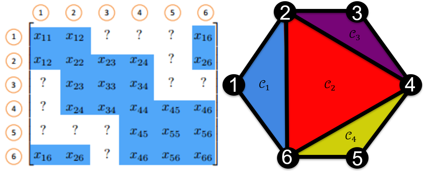
Figure 1: Left: A $6\times 6$ PSD completable cone $\mathbb{S}^{n}_{+}(\mathcal{E},?)$. Right: corresponding chordal graph $\mathcal{G}(\mathcal{V},\mathcal{E})$ with maximal cliques $\{\mathcal{C}_{k}\}_{k=1}^{4}$.

3.1 Definition of decomposed structured subsets

A clique edge cover of a graph $\mathcal{G}(\mathcal{V},\mathcal{E})$ is a set of subsets $\{\mathcal{C}_{k}\}_{k=1}^{p}$ such that every max. clique of $\mathcal{G}$ is contained in at least one clique $\mathcal{C}_{k}$. Clique edge covers allow for clique extensions and merges for possibly non-chordal graphs.

Definition 1.

We define sparse DD and SDD matrices as:

$$\mathcal{D}\mathcal{D}^{n}(\mathcal{E},0) =\mathbb{S}^{n}(\mathcal{E},0){\color[rgb]{0,0,0}\ \cap\ \mathcal{D}\mathcal{D}^{n}},$$

$$\mathcal{S}\mathcal{D}\mathcal{D}^{n}(\mathcal{E},0) =\mathbb{S}^{n}(\mathcal{E},0){\color[rgb]{0,0,0}\ \cap\ \mathcal{S}\mathcal{D}\mathcal{D}^{n}}.$$

These sparse matrices obey the containment:

$$\mathcal{D}\mathcal{D}^{n}(\mathcal{E},0)\subset\mathcal{S}\mathcal{D}\mathcal{D}^{n}(\mathcal{E},0)\subset\mathbb{S}^{n}_{+}(\mathcal{E},0).$$

The following result is proven in Appendix A:

Proposition 1.

Let $\mathcal{G}(\mathcal{V},\mathcal{E})$ be a graph with a clique edge cover $\{\mathcal{C}_{1},\mathcal{C}_{2},\ldots,\mathcal{C}_{p}\}$. Then,

1. $Z\in\mathcal{D}\mathcal{D}^{n}(\mathcal{E},0)$ iff

   $$Z=\textstyle\textstyle\sum_{k=1}^{p}{E_{\mathcal{C}_{k}}^{\mathsf{T}}Z_{k}E_{\mathcal{C}_{k}}},\quad Z_{k}\in\mathcal{D}\mathcal{D}^{|\mathcal{C}_{k}|},\;k=1,\,\ldots,\,p.$$

2. $Z\in\mathcal{S}\mathcal{D}\mathcal{D}^{n}(\mathcal{E},0)$ iff

   $$Z=\textstyle\textstyle\sum_{k=1}^{p}{E_{\mathcal{C}_{k}}^{\mathsf{T}}Z_{k}E_{\mathcal{C}_{k}}},\quad Z_{k}\in\mathcal{S}\mathcal{D}\mathcal{D}^{|\mathcal{C}_{k}|},\;k=1,\,\ldots,\,p.$$

Motivated by Theorems 1 and 2, and Proposition 1, we let $\mathcal{E}$ be a sparsity pattern, $\mathcal{K}=\{K_{k}\}_{k=1}^{p}$ be a set of cones corresponding to a clique edge cover $\mathcal{C}_{1},\ldots,\mathcal{C}_{p}$, where each individual cone $K_{k}$ is some structured subset in $\mathbb{S}^{|\mathcal{C}_{k}|}$. We define two decomposed structured subsets:

$$\mathcal{K}(\mathcal{E},0) :=\Big{\{}Z\in\mathbb{S}^{n}\mid Z=\sum_{k=1}^{p}{E_{\mathcal{C}_{k}}^{\mathsf{T}}Z_{k}E_{\mathcal{C}_{k}}},\Big{.}\;$$ (8)

. $$\qquad\qquad\qquad\qquad Z_{{}_{k}}\in K_{k},\;k=1,\,\ldots,\,p\Big{\}},$$

$$\mathcal{K}(\mathcal{E},?) :=\Big{\{}X\in\mathbb{S}^{n}\mid E_{\mathcal{C}_{k}}XE_{\mathcal{C}_{k}}^{\mathsf{T}}\in K_{k},\!k=1,\ldots,p\Big{\}}.$$

The decomposed structured subset $\mathcal{K}(\mathcal{E},0)$ generalizes $\mathcal{D}\mathcal{D}^{n}(\mathcal{E},0)$, $\mathcal{S}\mathcal{D}\mathcal{D}^{n}(\mathcal{E},0)$, and $\mathbb{S}^{n}_{+}(\mathcal{E},0)$ in the following sense:

$$\mathcal{K}(\mathcal{E},0) =\mathcal{D}\mathcal{D}^{n}(\mathcal{E},0), \text{if}\;K_{k}=\mathcal{D}\mathcal{D}^{|\mathcal{C}_{k}|},k=1,\ldots,p.$$

$$\mathcal{K}(\mathcal{E},0) =\mathcal{S}\mathcal{D}\mathcal{D}^{n}(\mathcal{E},0), \text{if}\;K_{k}=\mathcal{S}\mathcal{D}\mathcal{D}^{|\mathcal{C}_{k}|},k=1,\ldots,p.$$

If $$\mathcal{E}$$ is chordal, the additional results hold for PSD cones:

$$\mathcal{K}(\mathcal{E},0) =\mathbb{S}^{n}_{+}(\mathcal{E},0),\; \text{if}\;K_{k}=\mathbb{S}^{|\mathcal{C}_{k}|}_{+},k=1,\ldots,p,$$

$$\mathcal{K}(\mathcal{E},?) =\mathbb{S}^{n}_{+}(\mathcal{E},?),\; \text{if}\;K_{k}=\mathbb{S}^{|\mathcal{C}_{k}|}_{+},k=1,\ldots,p.$$

3.2 Containment Analysis

Definition 2.

For a graph $\mathcal{G}(\mathcal{V},\mathcal{E})$ with clique cover $\mathcal{C}_{1},\ldots,\mathcal{C}_{p}$, let $\mathcal{K}=\{K_{k}\}_{k=1}^{p}$ and $\tilde{\mathcal{K}}=\{\tilde{K}_{k}\}_{k=1}^{p}$ be two sets of clique-cones. The partial ordering $\subseteq$ is defined as:

$$\mathcal{K}\subseteq\tilde{\mathcal{K}}\quad\text{iff}\quad K_{k}\subseteq\tilde{K}_{k}\quad\forall\;k=1\ldots p.$$

Remark 1.

If clique-cones $\mathcal{K}\subset\tilde{\mathcal{K}}$ for a clique edge cover $\mathcal{C}_{1},\ldots,\mathcal{C}_{p}$ of a graph $\mathcal{G}(\mathcal{V},\mathcal{E})$, then by definition, we have

$$\mathcal{K}(\mathcal{E},0)\subseteq\tilde{\mathcal{K}}(\mathcal{E},0)\quad\text{and}\quad\mathcal{K}(\mathcal{E},?)\subseteq\tilde{\mathcal{K}}(\mathcal{E},?){\color[rgb]{0,0,0}.}$$

The relationship above is simple yet has useful implications in semidefinite optimization. In particular, the cone $\mathcal{D}\mathcal{D}^{n}(\mathcal{E},0)$ has the same cone on each clique $\mathcal{C}_{k}$ with $X_{k}\in\mathcal{D}\mathcal{D}^{\lvert\mathcal{C}_{k}\rvert}$. Mixing cones with $\mathcal{K}:K_{k}\supseteq\mathcal{D}\mathcal{D}^{\lvert\mathcal{C}_{k}\rvert},\forall k=1\ldots p$ where not all $K_{k}=\mathcal{D}\mathcal{D}^{\lvert\mathcal{C}_{k}\rvert}$ will form a cone $\mathcal{K}(\mathcal{E},0)\supset\mathcal{D}\mathcal{D}(\mathcal{E},0)$. Mixing cones therefore results in cones closer to $\mathbb{S}^{n}_{+}(\mathcal{E},0)$. Similar statements hold for $\mathbb{S}_{+}^{n}(\mathcal{E},?)$. This allows us to get better lower and upper bounds for problem (1). As an example, consider the following matrix parameterized by $(a,b)$:

$$M(a,b)=\begin{bmatrix}1&\frac{1}{2}+a&?&?\\ \frac{1}{2}+a&2&{-2a}&a+b\\ ?&{-2a}&5&\frac{b}{2}\\ ?&a+b&\frac{b}{2}&2\end{bmatrix},$$ (9)

where $?$ denotes unspecified entries. The sparsity pattern of $M(a,b)$ has two maximal cliques: $\{2,3,4\}$ and $\{1,2\}$. By Theorem 1, $M(a,b)\in\mathbb{S}_{+}^{4}(\mathcal{E},?)$ if:

$$M_{1}(a,b) =\begin{bmatrix}2&{-2a}&a+b\\ {-2a}&5&b/2\\ a+b&b/2&2\end{bmatrix}\succeq 0$$

$$M_{2}(a,b) =\begin{bmatrix}1&1/2+a\\ 1/2+a&2\end{bmatrix}\succeq 0.$$

Given a cone set $\mathcal{K}=\{\mathcal{K}_{1},\mathcal{K}_{2}\}$, we define the feasibility set for $M\in\mathcal{K}(\mathcal{E},?)$ as

$$\{(a,b)\mid M_{1}(a,b)\in\mathcal{K}_{1}\ \text{and}\ M_{2}(a,b)\in\mathcal{K}_{2}\}.$$

The black sets in Figure 2 are subsets of the $(a,b)$-plane where the matrix $M(a,b)$ has a PSD-completion ($M(a,b)\in\mathbb{S}_{+}(\mathcal{E},?)$). The blue feasibility sets are regions where $M_{1}(a,b)\in\mathcal{D}\mathcal{D}^{4}$ and $M_{2}(a,b)\in\mathcal{D}\mathcal{D}^{2}$. As expected, the blue set is contained within the black set since $\mathcal{D}\mathcal{D}^{4}(\mathcal{E},?)\subset\mathbb{S}_{+}^{4}(\mathcal{E},?)$. The orange set in the right panel has $M_{1}(a,b)\in\mathbb{S}^{3}_{+}$ and $M_{2}(a,b)\in\mathcal{D}\mathcal{D}^{2}$. Note how the orange set includes the blue set (all $\mathcal{D}\mathcal{D}$) and expands to nearly fill the left side of the black set (all $\mathbb{S}_{+}$). The green set in the left panel has $M_{2}(a,b)\in\mathbb{S}_{+}^{2}$ instead, which expands the $\mathcal{D}\mathcal{D}$ blue set with a small rightward bump.

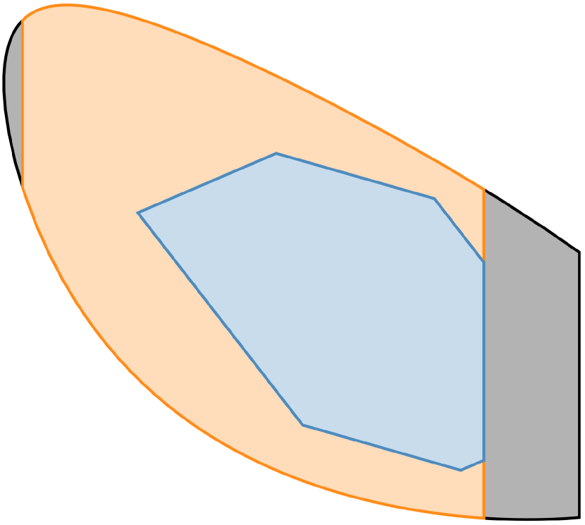
Figure 2: Mixing cones broadens feasibility regions for $M\in\mathcal{K}(\mathcal{E},?)$ in (9). Left: ${\color[rgb]{0.37109375,0.71875,0.359375}\mathcal{K}^{1}=\{\mathcal{D}\mathcal{D}^{3},\mathbb{S}_{+}^{2}\}}$; Right: ${\color[rgb]{1,0.546875,0.1015625}\mathcal{K}^{2}=\{\mathbb{S}_{+}^{3},\mathcal{D}\mathcal{D}^{2}\}}$.

Definition 3.

A sparse matrix $X\in{\color[rgb]{0,0,0}\mathbb{S}}^{n}(\mathcal{E},0)$ has a $K$-completion for a structured subset $K\subseteq\mathbb{S}_{+}^{n}$ if there exists an $\bar{X}\in K$ such that $X_{ij}=\bar{X}_{ij},\ \forall(i,j)\in\mathcal{E}$.

For a structured subset $K\subseteq\mathbb{S}_{+}^{n}$ and a sparsity pattern $\mathcal{G}(\mathcal{V},\mathcal{E})$, the set of $K$-completable matrices with pattern $\mathcal{E}$ is contained within $K(\mathcal{E},?)$. Figure 3 illustrates and compares feasibility sets for $M(a,b)\in K(\mathcal{E},?)$ (cliques of $M(a,b)$ in $K$) and when $M(a,b)$ has a $K$-completion. The blue $\mathcal{D}\mathcal{D}^{4}(\mathcal{E},?)$ and black $\mathbb{S}_{+}(\mathcal{E},?)$ feasibility set are the same in Figure 3 as in 2. The left panel additionally shows the feasible regions where $M(a,b)$ is $\mathcal{D}\mathcal{D}^{4}$-completable (red). The right plot echoes the left plot, where imposing that $M_{1}(a,b)\in\mathcal{S}\mathcal{D}\mathcal{D},M_{2}(a,b)\in\mathcal{S}\mathcal{D}\mathcal{D}$ yields a broader feasibility set than requiring that $M(a,b)$ has an $\mathcal{S}\mathcal{D}\mathcal{D}$-completion.

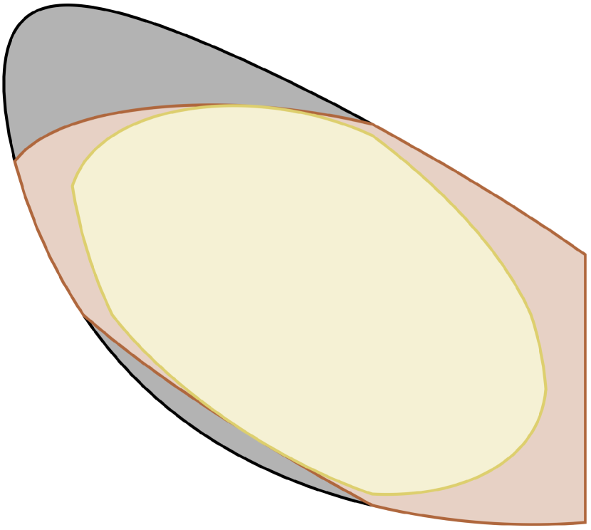
Figure 3: Regions of the $(a,b)$ plane for which the matrix $M(a,b)$ from Eq. (9) is ${\color[rgb]{0.90625,0.19140625,0.19921875}\mathcal{D}\mathcal{D}^{4}}$-completable, ${\color[rgb]{0.29296875,0.546875,0.75}\mathcal{D}\mathcal{D}^{4}(\mathcal{E},?)}$, or $\mathbb{S}^{4}_{+}(\mathcal{E},?)$ (Left), and ${\color[rgb]{0.86328125,0.8125,0.4296875}\mathcal{S}\mathcal{D}\mathcal{D}^{4}}$-completable, ${\color[rgb]{0.6875,0.40234375,0.2421875}\mathcal{S}\mathcal{D}\mathcal{D}^{4}(\mathcal{E},?)}$, or $\mathbb{S}_{+}^{4}(\mathcal{E},?)$ (Right). The containment of the plotted regions reflect the cone inclusions ${\color[rgb]{0.90625,0.19140625,0.19921875}\mathcal{D}\mathcal{D}^{4}}$-completable $\subset{\color[rgb]{0.29296875,0.546875,0.75}\mathcal{D}\mathcal{D}^{4}(\mathcal{E},?)}\subset\mathbb{S}^{4}_{+}(\mathcal{E},?)$ (Left); ${\color[rgb]{0.86328125,0.8125,0.4296875}\mathcal{S}\mathcal{D}\mathcal{D}^{4}}$-completable $\subset{\color[rgb]{0.6875,0.40234375,0.2421875}\mathcal{S}\mathcal{D}\mathcal{D}^{4}(\mathcal{E},?)}\subset\mathbb{S}_{+}^{4}(\mathcal{E},?)$ (Right).

Decomposed structured subsets can be posed over dual cones that are larger than the PSD cone.

Proposition 2.

Let $\mathcal{K}=\{K_{k}\}_{k=1}^{p}$ be a set of cones with dual $\mathcal{K}^{*}=\{K^{*}_{k}\}^{p}_{k=1}$, where $K_{k}$ is a structured subset in $\mathbb{S}^{|\mathcal{C}_{k}|}_{+}$ (i.e., $\mathcal{D}\mathcal{D}^{|\mathcal{C}_{k}|}$, $\mathcal{S}\mathcal{D}\mathcal{D}^{|\mathcal{C}|_{k}}$, or $\mathbb{S}^{|\mathcal{C}_{k}|}_{+}$), and $\mathcal{C}_{k}$ is a set of maximal cliques for $\mathcal{E}$. Then, we have

$$[\mathcal{K}(\mathcal{E},0)]^{*} =\mathcal{K}^{*}(\mathcal{E},?),$$ (10)

$$\qquad[\mathcal{K}(\mathcal{E},?)]^{*} \subseteq\mathcal{K}^{*}(\mathcal{E},0).$$ (11)

For the equivalence in Equation (10):

Proof.

Recall the definition of $\mathcal{K}(\mathcal{E},0)$ and $\mathcal{K}(\mathcal{E},?)$ in (8). We now verify that

$$[\mathcal{K}(\mathcal{E},0)]^{*}$$

$$= \{M\in\mathbb{S}^{n}\mid\langle M,N\rangle\geq 0,\forall N\in\mathcal{K}(\mathcal{E},0)\}$$

$$= \left\{M\in\mathbb{S}^{n}\mid\left\langle M,\sum_{k=1}^{p}E_{\mathcal{C}_{k}}^{\mathsf{T}}N_{k}E_{\mathcal{C}_{k}}\right\rangle\geq 0,\forall N_{k}\in K_{k}\right\}$$

$$= \left\{M\in\mathbb{S}^{n}\mid\sum_{k=1}^{p}\left\langle E_{\mathcal{C}_{k}}ME_{\mathcal{C}_{k}}^{\mathsf{T}},N_{k}\right\rangle\geq 0,\forall N_{k}\in K_{k}\right\}$$

$$= \left\{M\in\mathbb{S}^{n}\mid E_{\mathcal{C}_{k}}ME_{\mathcal{C}_{k}}^{\mathsf{T}}\in K_{k}^{*},k=1,\ldots,p\right\}$$

$$= \mathcal{K}^{*}(\mathcal{E},?),$$

where the second to last equality used the following fact: if any $E_{\mathcal{C}_{t}}ME_{\mathcal{C}_{t}}^{\mathsf{T}}\notin K_{t}^{*}$ for some $t$, we can choose $N_{t}\in K_{t}$ such that

$$\langle E_{\mathcal{C}_{t}}ME_{\mathcal{C}_{t}}^{\mathsf{T}},N_{t}\rangle<0.$$

Now, by choosing $N_{k}=0\in K_{k},k\neq t$, we have

$$\sum_{k=1}^{p}\left\langle E_{\mathcal{C}_{k}}ME_{\mathcal{C}_{k}}^{\mathsf{T}},N_{k}\right\rangle=\langle E_{\mathcal{C}_{t}}ME_{\mathcal{C}_{t}}^{\mathsf{T}},N_{t}\rangle<0,$$

which contradict line 4. Thus, we must have $E_{\mathcal{C}_{k}}ME_{\mathcal{C}_{k}}^{\mathsf{T}}\in K_{k}^{*},k=1,\ldots,p$.

∎

For the containment in Equation (11):

$$[\mathcal{K}(\mathcal{E},?)]^{*}=\mathcal{K}^{*}(\mathcal{E},0).$$

Proof.

Given any $M\in\mathcal{K}^{*}(\mathcal{E},0)$, we show $M\in[\mathcal{K}(\mathcal{E},?)]^{*}$. By definition (6), there exist $M_{k}\in K_{k}^{*},k=1,\ldots,p$, such that

$$M=\sum_{k=1}^{p}E_{\mathcal{C}_{k}}^{\mathsf{T}}M_{k}E_{\mathcal{C}_{k}}.$$

We now verify that $\forall N\in\mathcal{K}(\mathcal{E},?)$

$$\langle M,N\rangle =\left\langle\sum_{k=1}^{p}E_{\mathcal{C}_{k}}^{\mathsf{T}}M_{k}E_{\mathcal{C}_{k}},N\right\rangle$$

$$=\sum_{k=1}^{p}\left\langle M_{k},E_{\mathcal{C}_{k}}NE_{\mathcal{C}_{k}}^{\mathsf{T}}\right\rangle$$

$$=\sum_{k=1}^{p}\langle M_{k}\in K^{*}_{k},N_{k}\in K_{k}\rangle\quad\forall N_{k}\in K_{k}$$

$$\geq 0,$$

where the last inequality used the definition of $N\in\mathcal{K}(\mathcal{E},?)$. Thus, $M\in[\mathcal{K}(\mathcal{E},?)]^{*}$. We can conclude $\mathcal{K}^{*}(\mathcal{E},0)\subseteq[\mathcal{K}(\mathcal{E},?)]^{*}$ ∎

The reverse inclusion ($\mathcal{K}^{*}(\mathcal{E},0)\supseteq[\mathcal{K}(\mathcal{E},?)]^{*}$) is only guaranteed to hold if the clique cover $\mathcal{C}_{k}$ of $\mathcal{E}$ are disjoint: $\mathcal{C}_{k}\cap\mathcal{C}_{k^{\prime}}=\ \forall k\neq k^{\prime}$.

4 Applications to semidefinite optimization

In this section, we develop inner and outer approximations of semidefinite programs using the notion of decomposed structured subsets, and discuss an application of $\mathcal{H}_{\infty}$ norm estimation of network systems. All code is publicly available at https://github.com/zhengy09/SDPfw within the folder decomposed_structured_subsets.

4.1 Decomposed structured subsets in semidefinite programs

A semidefinite program in primal form (1) with $(X\in\mathbb{S}_{+}^{n})$ and dual form (1) $(Z\in\mathbb{S}_{+}^{n})$ will have matching optima $p^{*}=d^{*}$ when strong duality holds. By complementary slackness, $\langle X,Z\rangle=0$. Assume this semidefinite program has an aggregate sparsity pattern $\mathcal{E}$. With an optimization problem (1) over $X\in\mathbb{S}^{n}_{+}(\mathcal{E},?)$ and a cone set $\mathcal{K}$, an upper bound is attained by imposing $X\in\mathcal{K}(\mathcal{E},?)$ in (1), and a lower bound is found by restricting $Z\in\mathcal{K}(\mathcal{E},0)$ in (1).

The conic optimization problem (1) for a decomposed structured subset $\mathcal{K}(\mathcal{E},?)$ is:

$$\min_{X} \langle C,X\rangle$$ (12)

subject to $$\langle A_{i},X\rangle=b_{i},\;i=1,2,\ldots,m$$

$$E_{\mathcal{C}_{k}}XE_{\mathcal{C}_{k}}^{\mathsf{T}}\in K_{k}.$$

An example of decomposed structured subsets in action is a random SDP with block arrow sparsity pattern with 80 equality constraints, where each of the 15 blocks has size 10 and the arrowhead has width 10 (see Figure 4 for the aggregate sparsity pattern). The original SDP has $X\in\mathbb{S}_{+}^{160}$, and chordal decomposition has $X_{k}\in\mathbb{S}_{+}^{20}$ that are equal in the $10\times 10$ bottom right corner (blue pattern $\mathcal{E}$). A coarser chordal decomposition is the union of blue and magenta blocks in Figure 4 (fill-in $\mathcal{E}_{F}$), which has block sizes $(\mathbb{S}_{+}^{50})^{2}\times\mathbb{S}_{+}^{41}\times(\mathbb{S}_{+}^{30})^{2}$ that are each equal in the bottom right corner. Clique consistency for $\mathcal{E}_{F}$ adds 230 equality constraints, and for $\mathcal{E}$ adds 770.

Cost values of this SDP and its approximants are recorded in Table 1. Rows are different structured subsets and the columns apply the structured subsets: imposing that $X\in K$ and then that the cliques of $X_{k}\in K_{k}$, where cliques are set based on the graphs $\mathcal{E}_{F}$ and $\mathcal{E}$. We introduce shorthand $B_{k}$ as a cone of block factor-width 2 matrices where each block has $k$ components (so $B_{1}$ = $\mathcal{S}\mathcal{D}\mathcal{D}$) and membership constraints in $\mathbb{S}^{2k}_{+}$ are imposed. As an example, the row-column pair $(B_{5},K)$ corresponds to the cone $B_{5}^{160}$ and $(B_{1}0,K(\mathcal{E}_{F},?)$ refers to the cone $B_{1}0^{160}(\mathcal{E}_{F},?)$.’

By Agler’s theorem, all entries of $K=\mathbb{S}_{+}^{{\color[rgb]{0,0,0}160}}$ have the same optima. All entries $K=\mathcal{D}\mathcal{D}^{{\color[rgb]{0,0,0}160}}$ are infeasible, and objectives decrease towards the bottom right corner of the table as expected in the above containment analysis. Table 1 demonstrates that merging blocks together may degrade the resultant approximation quality. Merging strategies such as [13] must therefore be used with caution. Even well-chosen merges that speed up program execution may worsen the approximated SDP bound.

Figure 4: Block arrow sparsity pattern and extension

	$K$	$K(\mathcal{E}_{F},?)$	$K(\mathcal{E},?)$
$\mathcal{D}\mathcal{D}$	Inf.	Inf.	Inf.
$B_{1}$	64.5	34.7	19.4
$B_{2}$	51.4	27.1	13.9
$B_{5}$	32.1	15.0	5.34
$B_{10}$	20.8	7.10	-1.23
$\mathbb{S}_{+}$	-1.23	-1.23	-1.23

Table 1: Cost vs. subset and pattern in Fig. 4

4.2 Certifying Optimality

Karush-Kuhn-Tucker (KKT) conditions can be used to certify if an SDP approximated by structured subsets reaches the same cost as the original SDP [2]. For a cone $K\subset\mathbb{S}_{+}\subset K^{*}$ and an SDP of type (1), KKT relations on the left side will hold for an optimal primal-dual triple $(X,y,Z)\in(K^{n},\mathbb{R}^{m},K^{n^{*}})$ while optimizing over $X\in K$. All KKT conditions over $K$ in Equation (4.2) are also guaranteed to hold over $\mathbb{S}_{+}$ in Equation (4.2) except for dual feasibility ($Z\in K^{*}$):

$$X \in K$$

$$Z \in K^{*}$$ (13)

$$XZ =0$$

$$b_{i} =\langle A_{i},X\rangle\mid_{i=1}^{m}$$

$$C =S+\sum_{i=1}^{m}y_{i}A_{i},$$

$$X \in\mathbb{S}_{+}$$

$$Z \in\mathbb{S}_{+}$$ (14)

$$XZ =0$$

$$b_{i} =\langle A_{i},X\rangle\mid_{i=1}^{m}$$

$$C =S+\sum_{i=1}^{m}y_{i}A_{i}.$$

If the dual matrix $Z$ is PSD, then $(X,y,Z)$ solves the original SDP with the same optimal cost. Checking if $Z$ has a negative eigenvalue can be accomplished by inverse iteration (power method on $Z^{-1}$). SDP-optimality of decomposed structured subsets can be certified in the same framework given a set of clique cones $\mathcal{K}$. When finding lower bounds to semidefinite programs, the clique cones $\mathcal{K}$ have $K_{k}\supseteq\mathbb{S}_{+}$. Tightness is certified if each $X_{k}\in\mathbb{S}_{+}$. Upper bounds have $K_{k}\subseteq\mathbb{S}_{+}$. For each clique $\mathcal{C}_{k}$ in the clique cone $\mathcal{K}$, check if the corresponding dual block $Z_{k}\in\mathbb{S}_{+}$. The dual clique blocks $Z_{k}$ can be obtained by computing $Z=C-\sum_{i=1}^{m}{y_{i}A_{i}}$.

4.3 Decomposed Change of Basis

Decomposed structured subsets are compatible with the change of basis algorithm as reviewed in Section 2.1.1. Assume that $X_{0}\in\mathcal{K}(\mathcal{E},?)$ is a solution to Problem (1). Define Cholesky factorization matrices $L_{k}^{0}$ for each clique $k=1\ldots p$ such that $L_{k}^{0}L_{k}^{0{\mathsf{T}}}=E_{\mathcal{C}_{k}}X_{0}E_{\mathcal{C}_{k}}^{\mathsf{T}}$. The next iteration of the change of basis algorithm will solve

$$X_{1}=\arg\min_{X} \langle C,X\rangle$$ (15)

s.t. $$\langle A_{i},X\rangle=b_{i},\;i=1,2,\ldots,m$$

$$E_{\mathcal{C}_{k}}XE_{\mathcal{C}_{k}}^{\mathsf{T}}\in K_{k}(L_{k}^{0}).$$

The solution to (15) can be used to find a new set of factor matrices $L^{1}_{k}$ by finding $L_{k}^{1}L_{k}^{1{\mathsf{T}}}=E_{\mathcal{C}_{k}}X_{1}E_{\mathcal{C}_{k}}^{\mathsf{T}}$. Each clique $\mathcal{C}_{k}$ is described by basis $L_{k}$, and different bases may describe the same elements of $X$ on clique-overlaps.

Remark 2.

Performing a decomposed change-of-basis over $K^{n}(\mathcal{E},?)$ will result in a lower cost as compared to applying change-of-basis over $K^{n}$ at the first iteration. No conclusions can be drawn after the first iterations. In experiments, the cost sequence obtained from performing change-of-basis over $K^{n}$ remains above $K^{n}(\mathcal{E},?)$’s cost sequence.

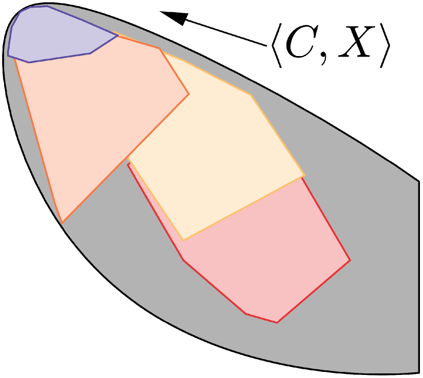
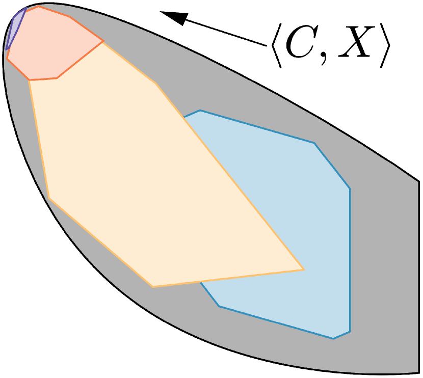
Figure 5: Decomposed vs. Standard Change of Basis on (9). Left: Start from ${\color[rgb]{0.90625,0.19140625,0.19921875}\mathcal{D}\mathcal{D}^{4}}$; Right: Start from ${\color[rgb]{0.29296875,0.546875,0.75}\mathcal{D}\mathcal{D}^{4}(\mathcal{E},?)}$.

Figure 5 illustrates the change of basis technique on a standard (left) and decomposed (right) structured subsets in the direction of $\langle C,X\rangle$. The intermediate costs are recorded in Table 2 for the first three iterations:

Table 2: Decreasing costs over Change of Basis

	Change of Basis Iteration
	0	1	2	3
$\mathcal{D}\mathcal{D}^{4}$	-1.41	-2.50	-3.08	-3.15
$\mathcal{D}\mathcal{D}^{4}(\mathcal{E},?)$	-1.41	-3.02	-3.13	-3.17

Figure 6 shows the output of the change of basis algorithm for the cone $B_{5}^{{\color[rgb]{0,0,0}160}}$ on the block arrow system shown in Figure 4. Over the course of 20 iterations, the basis-changed cone starting with $B_{5}^{{\color[rgb]{0,0,0}160}}(\mathcal{E},?)$ (green curve) eventually matches the SDP optimum.

Figure 6: Change of basis on Block Arrow SDP

A similar process can be done over the sparse cone $Z\in\mathcal{K}(\mathcal{E},0)$ (dual SDP), where bases $\mathcal{L}=\{L_{k}\}_{k=1}^{p}$ are tracked for each clique component $Z_{k}$ forming the clique-sum $Z=\sum_{k}{E_{\mathcal{C}_{k}}^{\mathsf{T}}Z_{k}E_{\mathcal{C}_{k}}}$ for $Z\in\mathcal{K}(\mathcal{L})(\mathcal{E},0)$.

4.4 H-infinity Norm Estimation for Networked Systems

Here, we present a special applications of SDPs in $\mathcal{H}_{\infty}$ norm estimation. Consider a state-space stable dynamical system $G(s)$:

$$\dot{x} =Ax+Bu,$$

$$y =Cx+Du.$$

The $\mathcal{H}_{\infty}$ norm of $G(s)$ is the supremum over frequencies $\omega$ of the maximum singular value of $G(j\omega)$. The norm $\lVert G\rVert_{\infty}$ is finite when $A$ is Hurwitz. The Bounded Real Lemma can be used to find upper bounds on $\lVert G\rVert_{\infty}$:

Theorem 3 (Bounded Real Lemma [9]).

The following statements are equivalent:

1. $\lVert G\rVert_{\infty}<\gamma,$

2. There exists a $P\succ 0$ such that

   $$\begin{bmatrix}PA+A^{\mathsf{T}}P+C^{\mathsf{T}}C&P^{\mathsf{T}}B+C^{\mathsf{T}}D\\ B^{\mathsf{T}}P+D^{\mathsf{T}}C&-\gamma^{2}I\end{bmatrix}\prec 0.$$

If the dynamical system is sparse (has a network structure), a dense $P\succ 0$ will give the tightest $H_{\infty}$ approximation but will destroy the sparsity pattern. Choosing a $P$ structure to be compatible with the LMI sparsity pattern will form a computationally tractable upper bound of $\lVert G(s)\rVert_{\infty}$. One structure on a block-diagonal $P$ that respects the network sparsity pattern is when the size of each agent’s block in $P$ equals its number of states [44].

As an example of applying decomposed structured subsets to $\mathcal{H}_{\infty}$ estimation, we present the ‘sea star’ networked system. The sea star system is composed of a set of agents clustered into a head and a set of arms. Each agent has internal linear dynamics ($n_{i}$ states, $m_{i}$ inputs, $d_{i}$ outputs), and they communicate and respond to a sparse selection of other agents. The left panel of Figure 7 shows a sea star network with 70 densely connected agents in the head and other agents distributed into 12 arms. Each arm is composed of 2 densely connected ‘knuckles’. Each knuckle has 10 agents, and every knuckle in the arm communicates with 4 agents in the next and previous knuckle (or the head as appropriate). The individual agent dynamics combine to form global dynamics $[A,B,C,D]$, where $A$ is Hurwitz.

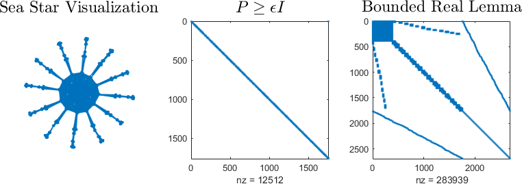
Figure 7: Sea Star network topology and LMI sparsity

Estimating $\lVert G(s)\rVert_{\infty}=\lVert C(sI-A)^{-1}B+D\rVert_{\infty}$ can be accomplished by using the bounded real lemma to minimize $\gamma^{2}$. The resultant LMI has two semidefinite variables, and the center and right panels of Figure 7 displays the sparsity pattern of constraints on these variables. The top left corner of the Bounded Real LMI shows a structure induced by the network interconnections. On their own, the two semidefinite blocks are of size 1760 and 2691.

This LMI system strongly exhibits chordal sparsity with edges $\mathcal{E}$, and can be posed as an optimization problem over the cone $\mathbb{S}_{+}(\mathcal{E},0)$. $\lvert\mathcal{C}_{k}\rvert$ is shown in Figure 8. There is a run of cliques of sizes ranging from 1-11, a set of cliques from sizes 37-90, and a solitary clique of size 387.

Figure 8: Maximal cliques of $\mathcal{E}$ from LMI with size thresholds

Results of $\mathcal{H}_{\infty}$ norm estimation of the sea star system are presented in Figures 3, 4, and 5. Columns are cones $K$ where $K=\mathcal{D}\mathcal{D}$ or $K=B_{q}$ if $q$ is an integer 2.1. Rows are size thresholds: the cone $K(\mathcal{E},0)$ has all cliques in $K$, and $\mathcal{K}_{60}(\mathcal{E},0)$ is a mixed cone where cliques with $\lvert\mathcal{C}\rvert\leq 60$ are PSD and $\lvert\mathcal{C}\rvert>60$ are in $K$. All experiments were written in MatlabR2018a and performed on Mosek [6] on a Intel i7 CPU with a clock frequency of 2.7GHz and 16.0 GB of RAM.

Table 3: Time to find $\gamma$ by upper bound $K$ (minutes)

Times in Figure 3 were measured solving the primal program over $K$. All displayed values achieved the SDP optimal solution, as certified in Section 4.2. The cones $\mathcal{D}\mathcal{D}$ with size thresholds 0 and 11 were primal infeasible, other non-displayed values did not attain the optimal $\gamma=1.137$. The cone $B_{5}$ was fastest at 1.84 minutes.

Table 4: $\gamma$ found by lower bound $K^{*}$

Table 5: Time to find lower bound $\gamma$ over $K^{*}$ (minutes)

Figure 4 displays lower bounds for $\gamma$ by over the dual cone $\mathcal{K}^{*}(\mathcal{E},0)$. Lower bounds tighten as cone complexity and size thresholds increase. The true $\gamma$ is obtained with a block-size of 55 and size-thresholds of 60 and 100 taking 34.8 and 34.0 minutes. Figure 5 contains the time taken to find all lower bounds. The computer running experiments ran out of memory attempting to solve the LMI over $\mathbb{S}_{+}(\mathcal{E},0)$.

5 Applications to Polynomial Optimization

This section reviews sum-of-squares methods for approximating the optimal values of polynomial optimization problems, and demonstrates how decomposed structured subsets may be applied.

5.1 Preliminaries for Polynomial Optimization

A polynomial optimization problem may be approximated by semidefinite programming. Other methods include using nonsymmetrtic cone optimization [28], applying Sketchy-CGAL [41] under limited memory requirements and low rank SDP solution structure, and exploiting the Constant Trace Property of moment relaxations [23, 22].

The task of minimizing a polynomial $p(x)\in\mathbb{R}[x]_{\leq d}$ of bounded degree $d$ is equivalent to solving [21]:

$$p^{*}= \max_{\gamma}{\gamma}$$ (16)

$$p(x)-\gamma\geq 0.$$

The imposition of a polynomial nonnegativity constraint is generically NP hard. Sum-of-squares (SOS) methods offer a convex relaxation of polynomial nonnegativity through SDPs. The square of a real number is always nonnegative, so a polynomial $q(x)=\sum_{i}\sigma_{i}(x)^{2}$ for polynomoials $q(x)\mathbb{R}[x]$ is also nonnegative. The cone of SOS polynomials $q(x)\in\Sigma[x]_{\leq d}$ is the set of polynomials of degree $\leq d$ that admit such a decomposition into terms $q(x)$. If $v_{d}(x)$ denotes a monomial map lifting $x$ into a set monomials up to degree $d$, then every SOS polynomial $\sigma(x)\in\Sigma[x]_{\leq d}$ has an equivalent description of $\sigma(x)=v(x)^{\mathsf{T}}Qv(x)$ for some $Q\succeq 0$. The SOS relaxation of degree $d$ of Equation (16) is:

$$p_{d}^{*}= \max_{\gamma}{\gamma}$$ (17)

$$p(x)-\gamma=\sigma(x)$$

$$\sigma(x)\in\Sigma[x]_{\leq d}.$$

Equation 17 is a semidefinite program in terms of the Gram matrix $Q$ that defines $\sigma(x)$. The coefficient matching conditions of $p(x)-\gamma=\sigma(x)$ are linear constraints in the entries of $Q$. Given an optimal $Q$, the SOS decomposition of $\sigma(x)$ can be recovered by a matrix factorization of $Q$ (e.g. Cholesky). The sequence $\{p_{d}^{*}\}$ is a increasing set of lower bounds to $p^{*}$.

Constrained polynomial optimization can be approached through SOS methods. A basic semialgebraic set $\mathbb{K}$ is defined by a finite number of bounded-degree polynomial inequality and equality constraints:

$$\mathbb{K}=\{x\mid g_{i}(x)\geq 0,\quad h_{j}(x)=0\}.$$ (18)

More generally, a semialgebraic set is the closure of basic semialgebraic sets under finite unions and projections down to coordinates. A constrained polynomial optimization problem can be formulated as Equation 16 with the added condition that $x\in\mathbb{K}$. If there exists a sufficiently large constant $R$ such that $\mathbb{K}\subset\{x\mid R-\lVert x\rVert_{2}^{2}\geq 0\}$, then the Putinar Positivstellensatz (Psatz) yields an equivalent formulation for polynomial constraint-multipliers $\zeta_{i}(x)$ and $\phi_{j}(x)$ [31]:

$$p^{*} =\max_{\gamma,\ \sigma,\ \zeta,\ \phi_{j}}{\gamma}$$ (19)

$$p(x)-\gamma=\sigma_{(}x)+\sum_{i}{\zeta_{i}(x)g_{i}(x)}+\sum_{j}{h_{j}(x)\phi_{j}(x)}$$

$$\sigma(x)\in\Sigma[x]\qquad\zeta(x)\in\Sigma[x]\qquad\phi_{j}(x)\in\mathbb{R}[x].$$

Equation (19) is an SDP when restricted to polynomials $\sigma(x),\zeta_{i}(x),\phi_{j}(x)$ of bounded degree $d$. If $\mathbb{K}$ satisfies an Archimedean condition then the sequence of lower bounds $p_{d}^{*}\leq p^{*}_{d+1}\leq\ldots$ will reach $p^{*}$ at a finite degree $d$ (Theorem 5.6 and 4.1 of [21]). The size of the Gram matrix $Q$ scales as $O(N^{d})$ for $x\in\mathbb{R}^{N}$, and SDP performance is polynomial in $N$ [21].

Utilizing sparsity in polynomial optimization can reduce computational complexity. Waki introduced a Correlative Sparsity Graph (CSP) $\mathcal{G}(\mathcal{V},\mathcal{E})$ where vertices $\mathcal{V}$ are variables $x_{i}$ in the problem. An edge $(x_{i},x_{j})\in\mathcal{E}$ appears if $x_{i}$ and $x_{j}$ are multiplied together in a monomial in the cost $p(x)$, or if they appear together in at least one constraint $g_{i}(x)$ or $h_{j}(x)$ [35]. Let $\mathcal{C}_{k}$ denote the cliques of the chordal-completed CSP graph, and $E_{k}x=x_{k}$ be the variables of $x$ present in CSP clique $\mathcal{C}_{k}$. The Putinar Psatz in Equation (19) can formulated as a sparse problem over per-clique polynomials [20]:

$$p^{*} =\max_{\gamma,\ \zeta_{i},\ \phi_{j}}{\gamma}$$ (20)

$$p(x)-\gamma=\sum_{k}\sigma_{k}(x)+\sum_{i,k}{\zeta_{ik}(x)g_{i}(x)}+\sum_{j,k}{h_{jk}(x)\phi_{j}(x)}$$

$$\zeta_{ik}(x_{k})\in\Sigma[x_{k}]\qquad\sigma_{k}(x_{k})\in\Sigma[x_{k}]\qquad\zeta_{ik}(x)\in\Sigma[x_{k}].$$

If the size of the largest CSP clique has cardinality $\kappa$, then the Psatz of degree $d$ in equation (20) will have expected $O(\kappa^{d})$ complexity. Other methods allow for decompositions according to the monomial structure in constraints. Josz uses monomial sparsity, which is a subset of the correlative sparsity graph [18]. Wang introduced a Term sparsity graph (TSSOS) based on links between monomials. The term sparsity graph allows for moment matrices to be block-diagonalized with an equivalent and mutually recoverable objective as SOS program [37]. Term sparsity may be combined with Correlative Sparsity to maximize performance [38]. Each of these methods use the structure of $p(x)$ and $\mathbb{K}$ to form computationally efficient semidefinite programs for polynomial optimization. Another cone for sparse POP approximation as an alternative to SOS polynomials is the Sum of Nonnegative Circuit polynomials [17, 11, 36].

5.2 Decomposed Structured Subsets for POPs

Computational complexity can also be reduced by restricting polynomials to structured subsets. Given that $p(x)\in SOS$ implies that $p(x)=v(x)^{\mathsf{T}}Qv(x),\ Q\geq 0$, setting $Q\in\mathcal{D}\mathcal{D}$ or $Q\in\mathcal{S}\mathcal{D}\mathcal{D}$ results in polynomial cones $p(x)\in DSOS$ or $p(x)\in SDSOS$ respectively [24].

Decomposed structured subsets can be integrated into polynomial optimization. For a single SOS polynomial $p(x)\in SOS$, with chordal Gram sparsity pattern $\mathcal{G}(\mathcal{V},\mathcal{E})$ and maximal cliques $\{\mathcal{C}_{k}\}_{k=1}^{p}$, Agler’s theorem forms an equivalence of optima between $Q\in\mathbb{S}_{+}^{n}$ and $Q\in\mathbb{S}_{+}^{n}(\mathcal{E},0)$. Restricting to standard structured subsets $p(x)\in DSOS$ forms $Q\in(\mathcal{D}\mathcal{D}\cap\mathbb{S}^{n}(\mathcal{E},0))=\mathcal{D}\mathcal{D}^{n}(\mathcal{E},0)$, and likewise $p(x)\in SDSOS$ forms $Q\in(\mathcal{S}\mathcal{D}\mathcal{D}\cap\mathbb{S}^{n}(\mathcal{E},0))=\mathcal{S}\mathcal{D}\mathcal{D}^{n}(\mathcal{E},0)$. Allowing for mixed clique cones yields $\mathcal{K}(\mathcal{E},0)$, which may be broader than $\mathcal{D}\mathcal{D}(\mathcal{E},0)$ or $\mathcal{S}\mathcal{D}\mathcal{D}(\mathcal{E},0)$ alone.

An example of decomposed structured subsets for polynomial optimization is the minimization of the (Rosenbrock-inspired) polynomial $f(x)=f_{Q}(x)+f_{R}(x)$, where

$$f_{R}(x) =\sum_{i=1}^{N-3}{10(x_{i+2}+2x_{i+1}-x_{i}^{2})^{2}+(1-x_{i}-x_{i+3})^{2}},$$

$$f_{Q}(x) =x_{1:N/6}^{\mathsf{T}}Ax_{1:N/6}.$$

$f_{Q}(x)$ is a quadric where $A$ is the Lerner matrix defined as $\text{min}(i/j,j/i)$. With an 120 variable problem, the correlative sparsity graph of the Lehmer-Rosenbrock (LR) function $f(x)$ has cliques with size $\{4,8,11,15,231\}$. The size 15 occurs 97 times and all other clique sizes appear once. The Lehmer-Rosenbrock function is chosen to highlight a set of SDPs with one very large clique. The standard Rosenbrock function is highly sparse, and does not have one giant component.

Table 6 shows the results of this optimization for the correlative sparsity pattern based on Sparse Sum of Squares [42]. This method is based on the sparsity of the Gram matrix $Q$ and optimizes over the cone of SOS polynomials of bounded degree. Table 6 therefore shows a hierarchy of lower bounds to the minimum of $f(x)$ on $\mathbb{R}^{120}$. In the Cost and Time section, $K(\mathcal{E},0)$ is the cone where all cliques are in $K$, and $\mathcal{K}(\mathcal{E},0)$ is the cone where the largest (231-sized) clique is in $K$ and all other cliques are in $\mathbb{S}_{+}$. Upper bounds in this context would approximate the second-order moment relaxation, and would not give any useful bounds on the true polynomial optimum. Cells are merged if the cones are equal (as implemented).

Table 6: CSP $f(x)$ Lower Bounds

	Cost		Time (s)
Cone	$K^{*}(\mathcal{E},0)$	$\mathcal{K}^{*}(\mathcal{E},0)$	$K^{*}(\mathcal{E},0)$	$\mathcal{K}^{*}(\mathcal{E},0)$
$\mathcal{D}\mathcal{D}$	-Inf.	-Inf.	0.75	0.86
$\mathcal{S}\mathcal{D}\mathcal{D}$	-113.91	-111.25	42.8	33.2
$B_{2}$	-111.63	-111.19	15.7	12.6
$B_{3}$	-111.52	-111.18	12.5	12.0
$B_{5}$	-111.06	-111.05	12.75	12.6
$B_{11}$	-110.85		27.1
$B_{21}$	-110.39		45.9
$B_{40}$	-110.26		112.7
$\mathbb{S}_{+}$	-110.20		219.6

Constrained polynomial optimization offers additional freedom of cone-selection for decomposed structured subsets. Cones in $\mathcal{K}$ can be chosen for each SOS constrained polynomial $p(x)$ and $\sigma_{i}(x)$. The following examples cover minimizing $f(x)$ over the semialgebraic set $x_{i}\in[1,2]$. This region can be represented as $\mathbb{K}=\{g_{i}(x)=(x-1)(2-x)\geq 0\}$. TSSOS [37] supports constrained polynomial optimization problems and exploits term sparsity in the constraint functions $g(x)$. The TSSOS clique sizes of minimizing the LR function $f(x)$ over $\mathbb{R}^{120}$ (unconstrained) and over $\mathbb{K}$ (constrained) in the $d=2$ level of the Lasserre hierarchy are displayed in Figure 9. This decomposition was obtained after the block hierarchy stabilized using the ‘clique’ option in the TSSOS Julia implementation. TSSOS resulted in smaller clique sizes (compare 121 for TSSOS vs. 231 for CSP) as shown in Figure 9 at the expense of preprocessing time.

Figure 9: Cliques for LR TSSOS unconstrained and constrained optimization.

Figures 7 and 8 display the time taken to provide lower bounds of $f(x)$ over the regions $\mathbb{R}^{120}$ and $[1,2]^{120}$ at the second Moment relaxation. Time is labeled in minutes to best provide contrast and intuition. Only values achieving the SDP optimum are displayed. In the constrained case, the lower bound of 4939.1 is attained in 31.8 minutes with the cone $B_{3}^{*}$ and size threshold 45, compared to 63.4 minutes on the full SDP $\mathbb{S}_{+}(\mathcal{E},?)$.

Table 7: Time to find unconstrained LR lower bound by TSSOS over $K^{*}$ (minutes)

Table 8: Time to find constrained LR lower bound by TSSOS over $K^{*}$ (minutes)

6 Conclusions

Structured subsets can be used to find upper and lower bounds of SDP optima. Decomposition methods may be able to convert large PSD constraints into smaller PSD blocks. This paper combines the two methods into decomposed structured subsets. Properties of these subsets are analyzed with their bound quality, and the facility to mix cones adds additional flexibility. Improved approximations are demonstrated on $\mathcal{H}_{\infty}$ norm and polynomial optimization problems. Future directions include applying these techniques to network $\mathcal{H}_{\infty}$-optimal control and more POPs. It would also be valuable to investigate compromises between cone complexity, additional consistency constraints, and approximation quality.

Appendix A Proof of Proposition 1

In this Appendix, we provide the proof for Proposition 1 where $\mathcal{E}$ is not necessarily a chordal graph.

$\Leftarrow:$ If $Z_{k}\in\mathcal{D}\mathcal{D}^{|\mathcal{C}_{k}|}$ then ${E_{\mathcal{C}_{k}}^{\mathsf{T}}Z_{k}E_{\mathcal{C}_{k}}}\in\mathcal{D}\mathcal{D}^{n}$ because diagonal elements of $Z_{k}$ will remain on the diagonal of ${E_{\mathcal{C}_{k}}^{\mathsf{T}}Z_{k}E_{\mathcal{C}_{k}}}$, and the diagonal dominance relation is preserved in the embedded matrix. $\mathcal{D}\mathcal{D}^{n}$ is a cone, so $Z=\sum_{k=1}^{p}{E_{\mathcal{C}_{k}}^{\mathsf{T}}Z_{k}E_{\mathcal{C}_{k}}}\in\mathcal{D}\mathcal{D}^{n}$ for multiple cliques in $\mathcal{C}$. Let $\mathcal{E}^{c}\supseteq\mathcal{E}$ be a chordal completion of $\mathcal{E}$ with a clique cover $\mathcal{C}^{c}$. All of the induced submatrices of $Z$ by cliques in $\mathcal{C}^{c}$ are $DD$, so from Agler’s theorem we have $Z\in\mathbb{S}^{n}(\mathcal{E},0)$. Thus, $Z\in\mathcal{D}\mathcal{D}^{n}(\mathcal{E},0)$.

$\Rightarrow:$ Let $e_{i}\in\mathbb{R}^{n},e_{j}\in\mathbb{R}^{n}$ where $i\neq j$ be standard basis vectors, we define the following $DD$ basis matrices:

$$v_{i} =e_{i}e_{i}^{\mathsf{T}}, v^{\pm}_{ij} =(e_{i}\pm e_{j})(e_{i}\pm e_{j})^{\mathsf{T}}.$$

Given a symmetric $Z\in\mathcal{D}\mathcal{D}^{n}(\mathcal{E},0)$ for a (not-necessarily chordal) sparsity pattern $\mathcal{E}$, define the slack quantities $\Delta_{i}=Z_{ii}-\sum_{j\neq i}|Z_{ij}|\geq 0$. Such a $Z$ can be decomposed as:

$$Z =\textstyle\sum_{i=1}^{n}\Delta_{i}v_{i}+\textstyle\sum_{(i,j)\in\mathcal{P}}Z_{ij}v^{+}_{ij}+\textstyle\sum_{(i,j)\in\mathcal{N}}|Z_{ij}|v^{-}_{ij}$$

$$\mathcal{P} :=\{(i,j)\mid Z_{ij}>0,\ i<j\}$$

$$\mathcal{N} :=\{(i,j)\mid Z_{ij}<0,\ i<j\}.$$

By this characterization, $Z\in\mathcal{D}\mathcal{D}^{n}(\mathcal{E},0)$ can be represented as the sum of $DD$ matrices with the same pattern $\mathcal{E}$ and clique cover $\mathcal{C}$. The terms $v_{ij}^{+},\ v_{ij}^{-}$ with $Z_{ij}\neq 0$ can be uniquely assigned to some clique $(i,j)\in\mathcal{C}_{k}$, and the slack terms $\Delta_{i}v_{i}$ can be distributed among all cliques in $\mathcal{C}$ that include $i$. Grouping summands into cliques yields

$$Z =\textstyle\sum_{k=1}^{p}{E_{\mathcal{C}_{k}}^{\mathsf{T}}Z_{k}E_{\mathcal{C}_{k}}},\quad Z_{k}\in\mathcal{D}\mathcal{D}^{|\mathcal{C}_{k}|}, k=1,\,\ldots,\,p.$$

Let $D$ be a positive definite (PD) diagonal matrix, and define matrices $D_{\mathcal{C}_{k}}=E_{\mathcal{C}_{k}}DE_{\mathcal{C}_{k}}^{\mathsf{T}}$ with inverses $D_{\mathcal{C}_{k}}^{-1}=E_{\mathcal{C}_{k}}D^{-1}E_{\mathcal{C}_{k}}^{\mathsf{T}}$. By definition (3) there exists a PD diagonal matrix $D$ for a $Z\in\mathcal{S}\mathcal{D}\mathcal{D}^{n}(\mathcal{E},0)$ such that $DZD\in\mathcal{D}\mathcal{D}^{n}$. Since pre and post-multiplying by a diagonal matrix does not change the sparsity pattern, $DZD\in\mathcal{D}\mathcal{D}^{n}(\mathcal{E},0)$. By the decomposition of $\mathcal{D}\mathcal{D}^{n}$ matrices:

$$DZD=\textstyle\sum_{k=1}^{p}{E_{\mathcal{C}_{k}}^{\mathsf{T}}\tilde{Z}_{k}E_{\mathcal{C}_{k}}},$$

where $\tilde{Z}_{k}\in\mathcal{D}\mathcal{D}^{\lvert\mathcal{C}_{k}\rvert},k=1,\ldots,p$. This leads to

$$Z=\textstyle\sum_{k=1}^{p}{D^{-1}E_{\mathcal{C}_{k}}^{\mathsf{T}}\tilde{Z}_{k}E_{\mathcal{C}_{k}}D^{-1}}=\sum_{k=1}^{p}{E_{\mathcal{C}_{k}}^{\mathsf{T}}{Z}_{k}E_{\mathcal{C}_{k}}},$$

where $Z_{k}=D^{-1}_{\mathcal{C}_{k}}\tilde{Z}_{k}D^{-1}_{\mathcal{C}_{k}}\in\mathcal{S}\mathcal{D}\mathcal{D}^{|\mathcal{C}_{k}|}$, since $E_{\mathcal{C}_{k}}D^{-1}=D^{-1}_{\mathcal{C}_{k}}E_{\mathcal{C}_{k}}$ and $D_{\mathcal{C}_{k}}^{-1}=E_{\mathcal{C}_{k}}D^{-1}E_{\mathcal{C}_{k}}^{\mathsf{T}}$, completing the proof.

Appendix B Combining Decompositions

This section of the appendix reviews symmetry and *-algebra structure, shows how these structures can be incorporated into the Decomposed Structured Subset framework, and demonstrates how exploiting multiple forms of structure results in finer approximations.

B.1 Symmetry/*-algebra Decomposition

An additional form of structure occurs when all constraint and cost matrices $(C,A_{i})$ can be simultaneously block diagonalized with a unitary matrix $P$:

$$\langle C,X\rangle=\langle P^{T}CP,\tilde{X}\rangle=\sum_{k}{\langle\tilde{C}_{k},\tilde{X}_{k}\rangle}\\$$

Application of $P$ effectively breaks the large PSD variable $X=P\tilde{X}P^{T}$ into a product of smaller PSD variables $\tilde{X_{k}}$, and the SDP in $(\tilde{C}_{k},\tilde{A_{i}}_{k})$ will have an equivalent optimum as $(C,A_{i})$. This block diagonalization can occur if all matrices $(C,A_{i})$ lie in a common *-algebra $\mathcal{A}$. *-algebras are subsets of matrices that are closed under addition, products, and transposition. If $(C,A_{i})$ are all symmetric of size $n$, the blocks are free symmetric matrices of size $n_{i}$ with multiplicity $m_{i}$. This is expressed in the Wedderburn decomposition [39]:

$$\mathcal{A}\cong\bigoplus_{i=1}^{p}{I_{m_{i}}\otimes S^{n_{i}}}\qquad\langle C,X\rangle=\sum_{i}m_{i}\langle\tilde{C}_{i},\tilde{X}_{i}\rangle$$

The Wedderburn decomposition of a *-algebra, given its basis, can be calculated numerically by randomized linear algebra [27]. Group-invariant SDPs are a specific case of *-algebra structure. The Wedderburn decomposition of $G$-invariant matrices is related to the isotypic decomposition, and if $G$ is known in advance, the block-diagonalizing matrix $P$ may be calculated explicitly. Jordan decomposition generalizes symmetry and *-algebra decomposition, and involves projections onto an invariant subspace followed by splitting into the product of Jordan subalgebras (also requiring randomized computation) [30]. While preprocessing group and *-algebra structure is usually more expensive than exploiting chordal decompositions, their block-diagonalizability ensures that there are no overlaps between blocks (unlike clique-consistency constraints).

If the semialgebraic set $\mathbb{K}$ is invariant under a symmetry group $G$, this structure can be exploited to reduce the computational burden. There exists an extensive literature on polynomial invariant and equivariant theory [32], and the main reference for SOS-based symmetry in polynomial optimization is [14]. The Hironaka decomposition of the invariant ring $\mathbb{R}[x]^{G}$ effects a block-diagonalization, which applies to $\mathbb{K}$ only if each polynomial $g_{i}(x),h_{j}(x)$ is invariant under $G$-actions. The methods of this paper can be applied after symmetry processing to restrict each block to a structured subsets, after first applying sparsity.

B.2 Symmetry structure

Decomposed structured subsets can be applied to symmetric SDPs in the same manner as chordally sparse problems. In the *-algebra framework, the cone-set $\mathcal{K}$ refers to the cone of each symmetric block in the program.

A semidefinite program may contain more than one kind of structure. Figure 10 shows block-arrow (sparse) matrices in the invariant ring $[\mathbb{S}^{90}]^{G}$ under block-permutation action. The permutation structure is illustrated in the top-left pane of Figure 10. Matrices $X\in[\mathbb{S}^{90}]^{G}$ are invariant under swapping blocks of the same color, and some blocks are additionally invariant under swapping the top and bottom halves (checkered pattern, split blocks). The permutation group $G$ acting on these matrices is:

$$G=(S_{4}\times\mathbb{Z}_{2})\times Id\times\mathbb{Z}_{2}\times\mathbb{Z}_{2}$$

The top right pane of Figure 10 shows a one such matrix $X\in[\mathbb{S}^{90}]^{G}$. All such matrices can be block diagonalized (bottom right) under unitary action by the matrix $P$ (bottom left, based on the Discrete Cosine Transform). The block-sizes and multiplicities are:

$$(m,n)=\{(3,5),(1,10),(4,5),(1,5),(1,40)^{sparse}\}$$

Table 9 shows the cost and time of running a randomly generated $G$-invariant SDP with 80 equality constraints under the cone $\mathcal{S}\mathcal{D}\mathcal{D}$. The columns show if the matrix has been block-diagonalized before applying $\mathcal{S}\mathcal{D}\mathcal{D}$, and the rows indicate if Grone’s theorem has been applied to apply $\mathcal{S}\mathcal{D}\mathcal{D}$ to cliques. (Full, Sparse) has the same cost as (Sym, Sparse), but takes longer to run because block-diagonalization eliminates redundancies in blocks with multiplicities. Wedderburn Decomposition, whole blocks (green, brown orbits) contribute blocks of size 10 while split blocks have block-sizes of 5.

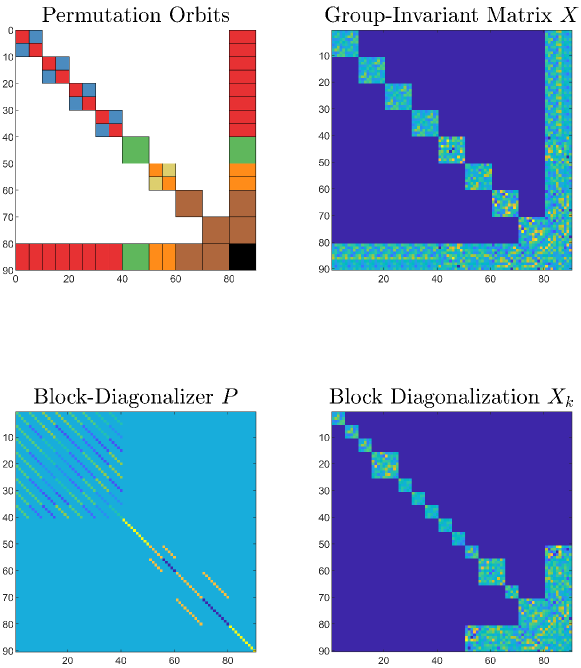
Figure 10: Sparse and Symmetric *-algebra

Table 9: $\mathcal{S}\mathcal{D}\mathcal{D}$ Block Arrow with Symmetry

Cost	Full	Sym.		Time (s)	Full	Sym.
Full	12.96	10.86		Full	124.5	19.3
Sparse	9.49	8.44		Sparse	38.2	12.0

References

- [1] Jim Agler, William Helton, and et al. Positive semidefinite matrices with a given sparsity pattern. Linear algebra and its applications, 107:101–149, 1988.
- [2] Amir Ali Ahmadi, Sanjeeb Dash, and Georgina Hall. Optimization over structured subsets of positive semidefinite matrices via column generation. Discrete Optim., 24:129–151, 2017.
- [3] Amir Ali Ahmadi and Georgina Hall. Sum of Squares Basis Pursuit with Linear and Second Order Cone Programming. In Algebraic and Geometric Methods in Discrete Mathematics, chapter 2, pages 27–54. AMS, Oxford, 4 2017.
- [4] Amir Ali Ahmadi and Anirudha Majumdar. Dsos and sdsos optimization: more tractable alternatives to sum of squares and semidefinite optimization. SIAM Journal on Applied Algebra and Geometry, 3(2):193–230, 2019.
- [5] Farid Alizadeh. Interior Point Methods in Semidefinite Programming with Applications to Combinatorial Optimization. SIAM J. Optim., 5(1):13–51, 1995.
- [6] Erling D Andersen and Knud D Andersen. The Mosek Interior Point Optimizer for Linear Programming: An Implementation of the Homogeneous Algorithm. In High performance optimization, pages 197–232. Springer, 2000.
- [7] George Barker and David Carlson. Cones of diagonally dominant matrices. PAC J. MATH, 57(1):15–32, 1975.
- [8] Erik G Boman, Doron Chen, Ojas Parekh, and Sivan Toledo. On factor width and symmetric H-matrices. Linear algebra and its applications, 405:239–248, 2005.
- [9] Stephen Boyd, Laurent El Ghaoui, Eric Feron, and Venkataramanan Balakrishnan. Linear Matrix Inequalities in System and Control Theory, volume 15. SIAM, 1994.
- [10] Stephen Boyd and Lieven Vandenberghe. Convex Optimization. Cambridge University Press, 2004.
- [11] Mareike Dressler, Janin Heuer, Helen Naumann, and Timo de Wolff. Global Optimization via the Dual SONC Cone and Linear Programming. In Proceedings of the 45th International Symposium on Symbolic and Algebraic Computation, pages 138–145, 2020.
- [12] K Fujisawa, S Kim, M Kojima, Y Okamoto, and M Yamashita. User’s manual for sparsecolo: Conversion methods for sparse conic-form linear optimization problems. Research Report B-453, Dept. of Math. and Comp. Sci. Japan, Tech. Rep., pages 152–8552, 2009.
- [13] Michael Garstka, Mark Cannon, and Paul Goulart. A clique graph based merging strategy for decomposable SDPs. IFAC-PapersOnLine, 53(2):7355–7361, 2020.
- [14] Karin Gatermann and Pablo A Parrilo. Symmetry groups, semidefinite programs, and sums of squares. J. Pure Appl. Algebra., 192(1-3):95–128, 2004.
- [15] Robert Grone, Charles R Johnson, Eduardo M Sá, and Henry Wolkowicz. Positive definite completions of partial Hermitian matrices. Linear Algebra Appl., 58:109–124, 1984.
- [16] Georgina Hall. Optimization over Nonnegative and Convex Polynomials With and Without Semidefinite Programming. arXiv preprint arXiv:1806.06996, 2018.
- [17] Sadik Iliman and Timo De Wolff. Lower Bounds for Polynomials with Simplex Newton Polytopes Based on Geometric Programming. SIAM J. Optim., 26(2):1128–1146, 2016.
- [18] Cédric Josz and Daniel K Molzahn. Lasserre Hierarchy for Large Scale Polynomial Optimization in Real and Complex Variables. SIAM J. Optim., 28(2):1017–1048, 2018.
- [19] Naonori Kakimura. A direct proof for the matrix decomposition of chordal-structured positive semidefinite matrices. Linear Algebra Appl., 433(4):819–823, 2010.
- [20] Jean B Lasserre. Convergent SDP-relaxations in polynomial optimization with sparsity. SIAM J. Optim., 17(3):822–843, 2006.
- [21] Jean-Bernard Lasserre. Moments, Positive Polynomials and Their Applications, volume 1. World Scientific, 2010.
- [22] Ngoc Hoang Anh Mai, Jean-Bernard Lasserre, Victor Magron, and Jie Wang. Exploiting constant trace property in large-scale polynomial optimization, 2020.
- [23] Ngoc Hoang Anh Mai, Victor Magron, and Jean-Bernard Lasserre. A hierarchy of spectral relaxations for polynomial optimization. arXiv preprint arXiv:2007.09027, 2020.
- [24] Anirudha Majumdar, Amir Ali Ahmadi, and Russ Tedrake. Control and verification of high-dimensional systems with DSOS and SDSOS programming. In 53rd IEEE Conference on Decision and Control, pages 394–401. IEEE, 2014.
- [25] Anirudha Majumdar, Georgina Hall, and Amir Ali Ahmadi. Recent Scalability Improvements for Semidefinite Programming with Applications in Machine Learning, Control, and Robotics. Annual Review of Control, Robotics, and Autonomous Systems, 3:331–360, 2020.
- [26] Jared Miller, Yang Zheng, Mario Sznaier, and Antonis Papachristodoulou. Decomposed Structured Subsets for Semidefinite Optimization. IFAC-PapersOnLine, 53(2):7374–7379, 2020. 21th IFAC World Congress.
- [27] Kazuo Murota, Yoshihiro Kanno, Masakazu Kojima, and Sadayoshi Kojima. A numerical algorithm for block-diagonal decomposition of matrix *-algebras with application to semidefinite programming. Japan Journal of Industrial and Applied Mathematics, 27(1):125–160, 2010.
- [28] Dávid Papp and Sercan Yildiz. Sum-of-squares optimization without semidefinite programming. SIAM J. Optim., 29(1):822–851, 2019.
- [29] Pablo A Parrilo. Structured Semidefinite Programs and Semialgebraic Geometry Methods in Robustness and Optimization. PhD thesis, California Institute of Technology, 2000.
- [30] Frank Permenter and Pablo A Parrilo. Dimension reduction for semidefinite programs via Jordan algebras. Mathematical Programming, pages 1–34, 2016.
- [31] Mihai Putinar. Positive Polynomials on Compact Semi-algebraic Sets. Indiana University Mathematics Journal, 42(3):969–984, 1993.
- [32] Bernd Sturmfels. Algorithms in invariant theory. Springer Science & Business Media, 2008.
- [33] Frank Vallentin. Symmetry in semidefinite programs. Linear Algebra Appl., 1(430):360–369, 2009.
- [34] Lieven Vandenberghe, Martin S Andersen, et al. Chordal Graphs and Semidefinite Optimization. Foundations and Trends in Optimization, 1(4):241–433, 2015.
- [35] Hayato Waki, Sunyoung Kim, Masakazu Kojima, and Masakazu Muramatsu. Sums of Squares and Semidefinite Program Relaxations for Polynomial Optimization Problems with Structured Sparsity. SIAM J. Optim., 17(1):218–242, 2006.
- [36] Jie Wang and Victor Magron. A second order cone characterization for sums of nonnegative circuits. In Proceedings of the 45th International Symposium on Symbolic and Algebraic Computation, pages 450–457, 2020.
- [37] Jie Wang, Victor Magron, and Jean-Bernard Lasserre. TSSOS: A Moment-SOS hierarchy that exploits term sparsity, 2019.
- [38] Jie Wang, Victor Magron, and Jean-Bernard Lasserre. Chordal-TSSOS: A Moment-SOS Hierarchy That Exploits Term Sparsity with Chordal Extension. SIAM J. Optim., 31(1):114–141, 2021.
- [39] Joseph Henry Maclagan Wedderburn. Lectures on Matrices, volume 17. American Mathematical Society, 1934.
- [40] Mihalis Yannakakis. Computing the Minimum Fill-In is NP-complete. SIAM J. Alg. Discr. Meth., 2(1), 1981.
- [41] Alp Yurtsever, Joel A Tropp, Olivier Fercoq, Madeleine Udell, and Volkan Cevher. Scalable Semidefinite Programming. SIAM Journal on Mathematics of Data Science, 3(1):171–200, 2021.
- [42] Y. Zheng, G. Fantuzzi, and A. Papachristodoulou. Sparse sum-of-squares (SOS) optimization: A bridge between DSOS/SDSOS and SOS optimization for sparse polynomials. In 2019 American Control Conference (ACC), pages 5513–5518, July 2019.
- [43] Yang Zheng, Giovanni Fantuzzi, Antonis Papachristodoulou, Paul Goulart, and Andrew Wynn. Chordal decomposition in operator-splitting methods for sparse semidefinite programs. Mathematical Programming, pages 1–44, 2019.
- [44] Yang Zheng, Maryam Kamgarpour, Aivar Sootla, and Antonis Papachristodoulou. Scalable analysis of linear networked systems via chordal decomposition. In 2018 European Control Conference (ECC), pages 2260–2265. IEEE, 2018.
- [45] Yang Zheng, Aivar Sootla, and Antonis Papachristodoulou. Block Factor-width-two Matrices and Their Applications to Semidefinite and Sum-of-squares Optimization. arXiv preprint arXiv:1909.11076, 2019.