Playing Games in the Dark: An approach for cross-modality transfer in reinforcement learning

Abstract.

In this work we explore the use of latent representations obtained from multiple input sensory modalities (such as images or sounds) in allowing an agent to learn and exploit policies over different subsets of input modalities. We propose a three-stage architecture that allows a reinforcement learning agent trained over a given sensory modality, to execute its task on a different sensory modality—for example, learning a visual policy over image inputs, and then execute such policy when only sound inputs are available. We show that the generalized policies achieve better out-of-the-box performance when compared to different baselines. Moreover, we show this holds in different OpenAI gym and video game environments, even when using different multimodal generative models and reinforcement learning algorithms.

1. Introduction

Recent works have shown how low-dimensional representations captured by generative models can be successfully exploited in reinforcement learning (RL) settings. Among others, these generative models have been used to learn low-dimensional latent representations of the state space to improve the learning efficiency of RL algorithms Zhang et al. (2018); Gelada et al. (2019), or to allow the generalization of policies learned on a source domain to other target domains Finn et al. (2016); Higgins et al. (2017). The DisentAngled Representation Learning Agent (DARLA) approach Higgins et al. (2017), in particular, builds such latent representations using variational autoencoder (VAE) methods Kingma and Welling (2013); Rezende et al. (2014), and shows how learning disentangled features of the observed environment can allow an RL agent to learn a policy robust to some shifts in the original domain.

In this work, we explore the application of these latent representations in capturing different input sensory modalities to be considered in the context of RL tasks. We build upon recent work that extends VAE methods to learn joint distributions of multiple modalities, by forcing the individual latent representations of each modality to be similar Suzuki et al. (2016); Yin et al. (2017). These multimodal VAEs allow for cross-modality inference, replicating more closely what seems to be the nature of the multimodal representation learning performed by humans Damasio (1989); Meyer and Damasio (2009). Inspired by these advances, we explore the impact of such multimodal latent representations in allowing a reinforcement learning agent to learn and exploit policies over different input modalities. Among others, we envision, for example, scenarios where reinforcement learning agents are provided the ability of learning a visual policy (a policy learned over image inputs), and then (re-)using such policy at test time when only sound inputs are available. Figure 1 instantiates such example to the case of video games—a policy is learned over images and then re-used when only the game sounds are available, i.e., when playing “in the dark”.

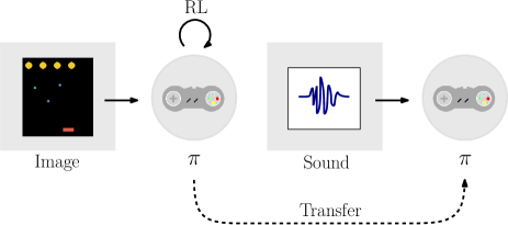
Figure 1. Concrete scenario where a policy trained over one input modality (game videoframes) is transferred to a different modality (game sound).

To achieve this, we contribute an approach for multimodal transfer reinforcement learning, which effectively allows an RL agent to learn robust policies over input modalities, achieving better out-of-the-box performance when compared to different baselines. We start by first learning a generalized latent space over the different input modalities that the agent has access to. This latent space is constructed using a multimodal generative model, allowing the agent to establish mappings between the different modalities—for example, “which sounds do I typically associate with this visual sensory information”. Then, in the second step, the RL agent learns a policy directly on top of this latent space. Importantly, during this training step, the agent may only have access to a subset of the input modalities (say, images but not sound). In practice, this translates in the RL agent learning a policy over a latent space constructed relying only on some modalities. Finally, the transfer occurs in the third step, where, at test time, the agent may have access to a different subset of modalities, but still perform the task using the same policy. These results hold consistently across different OpenAI Gym Brockman et al. (2016) and Atari-like Bellemare et al. (2013) environments. This is the case even when using different multimodal generative models Yin et al. (2017) and reinforcement learning algorithms Mnih et al. (2015); Lillicrap et al. (2015).

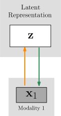
(a)

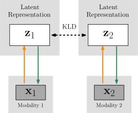
(b)

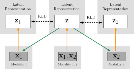
(c)

Figure 2. Networks of different generative models, highlighting the models’ data encoding (orange) and decoding (green) pipelines. The similarity constraints imposed by their training procedures are presented in dashed lines. 2(a)) The VAE model learns a latent representation of the data distribution of a single modality. 2(b)) On the other hand, the AVAE model extends the previous framework to account for multiple modalities, allowing for cross-modality inference. 2(c)) Finally, the JMVAE model learns a representation of both modalities, allowing for both single and joint modality reconstruction, and cross-modality inference.

The third and last step unveils what sets our work apart from the existing literature. By using (single-modality) VAE methods, the current state-of-art approaches implicitly assume that the source and target domains are characterized by similar inputs, such as raw observations of a camera. In these approaches, the latent space is used to capture isolated properties (such as colors or shapes) that may vary throughout the tasks. This is in contrast with our approach, where the latent space is seen as a mechanism to create a mapping between different input modalities.

The remainder of the paper is structured as follows. We start in Section 2 by introducing relevant background and related work on generative models and reinforcement learning. Then, in Section 3 we introduce our approach to multimodal transfer reinforcement learning, and evaluate it in Section 4. We finish with some final considerations in Section 5.

2. Preliminaries

This section introduces required background on deep generative models and deep reinforcement learning.

2.1. Deep Generative Models

2.1.1. Variational Autoencoders

Deep generative models have shown great promise in learning generalized representations of data. For single-modality data, the variational autoencoder model (VAE) is widely used. The VAE model Kingma and Welling (2013) learns a joint distribution $p_{\theta}(\boldsymbol{x},\boldsymbol{z})$ of data $\boldsymbol{x}$, which is generated by a latent variable $\boldsymbol{z}$. Figure 2(a) depicts this model. The latent variable is often of lower dimensionality in comparison with the modality itself, and acts as the representation vector in which data is encoded.

The joint distribution takes the form $p_{\theta}(\boldsymbol{x},\boldsymbol{z})=p_{\theta}(\boldsymbol{x}\,|\,\boldsymbol{z})\,p(\boldsymbol{z})$, where $p(\boldsymbol{z})$ (the prior distribution) is often a unitary Gaussian ($\boldsymbol{z}\sim\mathcal{N}(\boldsymbol{0},\boldsymbol{\mathrm{I}})$). The generative distribution $p_{\theta}(\boldsymbol{x}\,|\,\boldsymbol{z})$, parameterized by $\theta$, is usually composed with a simple likelihood term (e.g. Bernoulli or Gaussian).

The training procedure of the VAE model involves the maximization of the evidence likelihood $p(\boldsymbol{x})$, by marginalizing over the latent variable and resorting to an inference network $q_{\phi}(\boldsymbol{z}|\boldsymbol{x})$ to approximate the posterior distribution. We obtain a lower-bound on the log-likelihood of the evidence (ELBO) $\log p(\boldsymbol{x})\geq\mathcal{L}_{\text{VAE}}(\boldsymbol{x})$, with

$$\mathcal{L}_{\text{VAE}}(\boldsymbol{x})=\lambda\,\mathbb{E}_{q_{\phi}(\boldsymbol{z}|\boldsymbol{x})}\left[\log p_{\theta}(\boldsymbol{x}|\boldsymbol{z})\right]-\,\beta\,\operatorname{\mathbb{K}\mathbb{L}}\left[q_{\phi}(\boldsymbol{z}|\boldsymbol{x})\,\|\,p(\boldsymbol{z})\right],$$

where the Kullback-Leibler divergence term $\operatorname{\mathbb{K}\mathbb{L}}\left[q_{\phi}(\boldsymbol{z}|\boldsymbol{x})\,\|\,p(\boldsymbol{z})\right]$ promotes a balance between the latent channel’s capacity and the encoding process of data. Moreover, in the model’s training procedure, the hyperparameters $\lambda$ and $\beta$ weight the importance of reconstruction quality and latent space independence, respectively. The optimization of the ELBO is performed resorting to gradient-based methods.

2.1.2. Multimodal Variational Autoencoders

VAE models have been extended in order to perform inference across different modalities. The Associative Variational Autoencoder (AVAE) model Yin et al. (2017), depicted in Figure 2(b), is able to learn a common latent representation of two modalities ($\boldsymbol{x},\boldsymbol{y}$). It does so by imposing a similarity restriction on the separate single-modality latent representations ($\boldsymbol{z}_{x},\boldsymbol{z}_{y}$), employing a KL divergence term on the ELBO of the model:

$$\mathcal{L}_{\text{AVAE}}(\boldsymbol{x},\boldsymbol{y})=\mathcal{L}_{\text{VAE}}(\boldsymbol{x})+\mathcal{L}_{\text{VAE}}(\boldsymbol{y})-\,\alpha\operatorname{\mathbb{K}\mathbb{L}}^{\star}\left[q_{\phi}(\boldsymbol{z}_{x}|\boldsymbol{x})\,\|\,q_{\phi}(\boldsymbol{z}_{y}|\boldsymbol{y})\right]$$

where $\operatorname{\mathbb{K}\mathbb{L}}^{\star}\left[p\,\|\,q\right]$ is the symmetrical Kullback-Leibler between two distributions $p$ and $q$, and $\alpha$ is a constant that weights the importance of keeping similar latent spaces in the training procedure Yin et al. (2017). We note that each modality is associated with a different encoder-decoder pair. Moreover, the encoder and the decoder can be implemented as neural networks with different architectures.

Other models aim at learning a joint distribution of both modalities $p_{\theta}(\boldsymbol{x},\boldsymbol{y})$. Examples include the Joint Multimodal Variational Autoencoder (JMVAE) Suzuki et al. (2016) or the Multi-Modal Variational Autoencoder (M²VAE) Korthals (2019). These generative models are able to build a representation space of both modalities simultaneously while maintaining similarity restrictions with the single-modality representations, as shown in the JMVAE model presented in Figure 2(c).

However, a fundamental feature of all multimodal generative models is the ability to perform cross-modality inference, that is the ability to input modality-specific data, encode the corresponding latent representation, and, from that representation, generate data of a different modality. This is possible due to the forced approximation of the latent representations of each modality, and the process follows the orange and green arrows in Figure 2.

2.2. Reinforcement Learning

Reinforcement learning (RL) is a framework for optimizing the behaviour of an agent operating in a given environment. This framework is formalized as a Markov decision process (MDP)—a tuple $\mathcal{M}=(\mathcal{X},\mathcal{A},P,r,\gamma)$ that describes a sequential decision problem under uncertainty. $\mathcal{X}$ and $\mathcal{A}$ are the state and action spaces, respectively, and both are known by the agent. When the agent takes an action $a\in\mathcal{A}$ while in state $x\in\mathcal{X}$, the world transitions to state $y\in\mathcal{X}$ with probability $P(y\mid x,a)$ and the agent receives an immediate reward $r(x,a)$. Typically, functions $P$ and $r$ are unknown to the agent. Finally, the discount factor $\gamma\in[0,1)$ sets the relative importance of present and future rewards.

Solving the MDP consists in finding an optimal policy $\pi^{*}$—a mapping from states to actions—which ensures that the agent collects as much reward as possible. Such policy can be found from the optimal $Q$-function, which is defined recursively for every state action pair $\left(x,a\right)\in\mathcal{X}\times\mathcal{A}$ as

$$Q^{*}(x,a)=r(x,a)+\gamma\sum_{y\in\mathcal{X}}P(y\mid x,a)\max_{a^{\prime}\in\mathcal{A}}Q^{*}(y,a^{\prime}).$$

Multiple methods can be used in computing this function Sutton and Barto (1998), for example $Q$-learning Watkins (1989).

More recently, research has geared towards applying deep learning methods in RL problems, leading to new methods. For example, Deep $Q$ Network (DQN) is a variant of the $Q$-learning algorithm that uses a deep neural network to parameterize an approximation of the $Q$-functions $Q(x,a;\theta)$, with parameters $\theta$. DQN assumes discrete action spaces $\mathcal{A}$, and has been proved suitable for learning policies that beat Atari games Mnih et al. (2015). Continuous action spaces require specialized algorithms. For example, Deep Deterministic Policy Gradient (DDPG) is an actor-critic, policy gradient algorithm that can deal with continuous action spaces, and has been shown to perform well in complex control tasks Lillicrap et al. (2015).

3. Multimodal Transfer Reinforcement Learning

Consider an agent facing a sequential decision problem described as an MDP $\mathcal{M}=\left(\mathcal{X},\mathcal{A},P,r,\gamma\right)$. This agent is endowed with a set $\left\{I_{1},I_{2},\dots,I_{N}\right\}$ of $N$ different input modalities, which can be used in perceiving the world and building a possibly partial observation of the current state $x\in\mathcal{X}$. Different modalities may provide more, or less, perceptual information than others. Some modalities may be redundant (i.e., provide the same perceptual information) or complement each other (i.e., jointly provide more information). Figure 3 provides an abstract illustration of the connection between different input modalities, and corresponding impact in the state space that can be perceived by the agent.

Our goal is for the agent to learn a policy while observing only a subset of input modalities $\boldsymbol{I}_{\mathrm{train}}$, and then use that same policy when observing a possibly different subset of modalities, $\boldsymbol{I}_{\mathrm{test}}$, with as minimal performance degradation as possible.

Our approach consists of a three-stages pipeline:

1. Learn a perceptual model of the world.

2. Learn to act in the world.

3. Transfer policy.

We now discuss each step in further detail.

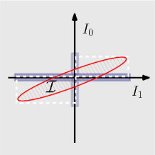
Figure 3. Connection between two abstract input modalities $I_{1}$ and $I_{2}$, and corresponding impact in the agent’s perceptual information. The elliptic surface $\mathcal{I}$ depicts the complete perceptual space the agent can perceive with both modalities. The colored projections in the axes depict the (reduced) perceptions of the agent when using single modalities.

3.1. Learn a perceptual model of the world

Let $\mathcal{I}$ denote the Cartesian product of input modalities, $\mathcal{I}=I_{1}\times I_{2}\times\dots\times I_{N}$. Intuitively, we can think of $\mathcal{I}$ as the complete perceptual space of the agent. We write $\boldsymbol{i}$ to denote an element of $\mathcal{I}$. Figure 4(a) depicts an example on a game, where the agent can have access to two modalities, $I_{\mathrm{image}}$ and $I_{\mathrm{sound}}$, corresponding to visual and sound information.

At each moment $t$, the agent may not have access to the complete perception $\boldsymbol{i}(t)\in\mathcal{I}$, but only to a partial view thereof. Following our discussion in Section 1, we are interested in learning a multimodal latent representation of the perceptions in $\mathcal{I}$. Such representation amounts to a set of latent mappings $\mathcal{F}=\{F_{1},\ldots,F_{L}\}$. Each map $F_{\ell}$ takes the form $F_{\ell}:\mathrm{proj}_{\ell}\to\mathcal{Z}$, where $\mathcal{Z}$ is a common latent space and $\mathrm{proj}_{\ell}$ projects $\mathcal{I}$ to some subspace of $K$ modalities, $\mathcal{I}_{\ell}=I_{\ell_{1}}\times I_{\ell_{2}}\times\ldots\times I_{\ell_{K}}$. In Figure 4(a) the set of mappings $\mathcal{F}$ is used to compute a latent representation $\boldsymbol{z}$ from sound and image data.

To learn such mappings, we start by collecting a dataset of $M$ examples of simultaneous sensorial information:

$$\mathcal{D}(\mathcal{I})=\big{\{}\boldsymbol{i}^{(1)},\ldots,\boldsymbol{i}^{(M)}\big{\}}.$$

We then follow an unsupervised learning approach, and train a multimodal VAE on dataset $\mathcal{D}(\mathcal{I})$ to learn a generalized latent space over the agent’s input modalities. The latent mappings in $\mathcal{F}$ correspond to the encoders of the VAE model, while the decoders can be seen as a set of inverse latent mappings, $\mathcal{F}^{-1}=\{F^{-1}_{1},\ldots,F^{-1}_{L}\}$ that allow for modality reconstruction and cross-modality inference. Figure 4(b) depicts an example of how the multimodal latent space can be used for performing cross-modality inference of sound data given an image input using the modality-specific maps.

The collection of the initial data needed to generate $\mathcal{D}(\mathcal{I})$ can be easier/harder depending on the complexity of the task. In Section 4 we discuss mechanisms to perform this.

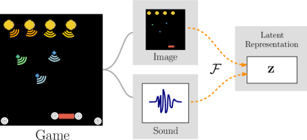
(a)

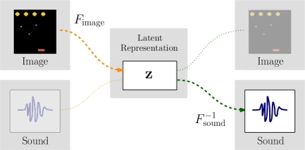
(b)

Figure 4. 4(a)) Each time step of a game includes visual and sound components that are intrinsically coupled. This coupling can be encoded in a latent representation using the family of latent maps $\mathcal{F}$. 4(b)) shows how the multimodal latent representation can be used in inferring the sound associated with a given image, using the image latent map $F_{\mathrm{image}}$ and sound inverse latent map $F_{\mathrm{sound}}^{-1}$.

3.2. Learn to act in the world

After learning a perceptual model of the world, the agent then learns how to perform the task. We follow a reinforcement learning approach to learn an optimal policy for the task described by MDP $\mathcal{M}$. During this learning phase, we assume the agent may only have access to a subset of input modalities $\boldsymbol{I}_{\mathrm{train}}$. As a result, during its interaction with the environment, the agent collects a sequence of triplets

$$\left\{\left(\boldsymbol{i}_{\mathrm{train}}^{(0)},a^{(0)},r^{(0)}\right),\left(\boldsymbol{i}_{\mathrm{train}}^{(1)},a^{(1)},r^{(1)}\right),\dots\right\},$$

where $\boldsymbol{i}_{\mathrm{train}}^{(t)}$, $a^{(t)}$, $r^{(t)}$ correspond to the perceptual observations, action executed, and rewards obtained at timestep $t$, respectively.

However, our reinforcement learning agent does not use this sequence of triplets directly. Instead, it pre-processes the perceptual observations using the previously learned latent maps $\mathcal{F}$ to encode the multimodal latent state at each time step as $\boldsymbol{z}^{(t)}=F_{\mathrm{train}}\left(\boldsymbol{i}_{\mathrm{train}}^{(t)}\right)$, where $F_{\mathrm{train}}\in\mathcal{F}$ maps $I_{\mathrm{train}}$ into $\mathcal{Z}$. In practice, the RL agent uses a sequence of triplets

$$\left\{\left(\boldsymbol{z}^{(0)},a^{(0)},r^{(0)}\right),\left(\boldsymbol{z}^{(1)},a^{(1)},r^{(1)}\right),\dots\right\}$$

to learn a policy $\pi:\mathcal{Z}\to\mathcal{A}$, that maps the latent states to actions. Any continuous-state space reinforcement learning algorithm can be used to learn this policy $\pi$ over the latent states. These latent states are encoded using the generative model trained in the previous section, and as such, the weights of this model should remain frozen during the RL training.

3.3. Transfer policy

The transfer of policies happens once the agent has learned how to perceive and act in the world. At this time, we assume the agent may now have access to a subset of input modalities $\boldsymbol{I}_{\mathrm{test}}$, potentially different from $\boldsymbol{I}_{\mathrm{train}}$, i.e., the set of modalities it used in learning the task policy $\pi$. As a result, during its interaction with the environment, at each time step $t$, the agent will now observe perceptual information $\boldsymbol{i}_{\mathrm{test}}^{(t)}$.

In order to reuse the policy $\pi$, the agent starts by pre-processing this perceptual observation, again using the set of maps $\mathcal{F}$ previously trained, but now generating a latent state $\boldsymbol{z}^{(t)}=F_{\mathrm{test}}\left(\boldsymbol{i}_{\mathrm{test}}^{(t)}\right)$, where $F_{\mathrm{test}}\in\mathcal{F}$ now maps $I_{\mathrm{test}}$ into $\mathcal{Z}$. Since policy $\pi$ maps the latent space $\mathcal{Z}$ to the action space $\mathcal{A}$, it can now be used directly to select the optimal action at the new state $\boldsymbol{z}^{(t)}$.

Effectively, the agent is reusing a policy $\pi$ that was learned over a (possibly) different set of input modalities, with no additional training. This corresponds to a zero-shot transfer of policies. Figure 5 summarizes the three-steps pipeline hereby described.

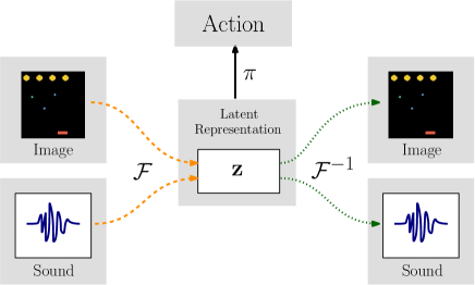
Figure 5. Summary of the three-steps approach for cross-modality transfer in reinforcement learning. The first step learns a perceptual model of the world, described by the latent mappings $\mathcal{F}$ (and corresponding inverses), which map perceptions to a common latent space $\mathcal{Z}$. In the second step, the agent learns a policy $\pi$ that maps the latent space to actions, with an RL approach using observations from a given subset of input modalities. The third step concerns the reuse off the same policy $\pi$, assuming new observations from a potentially different subset of modalities. This is possible by first encoding the new observations in the multimodal latent space.

4. Experimental Evaluation

We evaluate and analyze the performance of our approach on different scenarios of increasing complexity, not only on the task but also on the input modalities. We start by considering a modified version of the pendulum environment from OpenAI gym, with a simple sound source. Then, we consider hyperhot, a space invaders-like game that assesses the performance of our approach in scenarios with more complex and realistic generation of sounds.

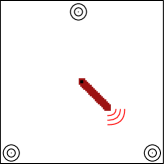
Figure 6. Visual and sound perceptual information in the pendulum scenario. The tip of the pendulum emits a frequency that is received by three microphones placed at the bottom left and right ($bl,br$) and middle top $(mt)$.

4.1. pendulum

We consider a modified version of the pendulum environment from OpenAI gym—a classic control problem, where the goal is to swing the pendulum up so it stays upright. We modify this environment so that the observations include both an image and a sound component. For the sound component, we assume that the tip of the pendulum emits a constant frequency $f_{0}$, which is received by a set of $S$ sound receivers $\left\{\rho_{1},\dots,\rho_{S}\right\}$. Figure 6 depicts this scenario, where the pendulum and its sound are in red, and the sound receivers correspond to the circles.

Formally, we let $\mathcal{I}=I_{\mathrm{image}}\times I_{\mathrm{sound}}$ denote the complete perceptual space of the agent. The visual input modality of the agent, $I_{\mathrm{image}}$, consists of the raw image observation of the environment. On the other hand, the sound input modality, $I_{\mathrm{sound}}$, consists of the frequency and amplitude received by each of the $S$ microphones of the agent. Moreover, both image and sound observations may be stacked to account for the dynamics of the scenario.

In this scenario, we assume a simple model for the sound generation. Specifically, we assume that, at each timestep, the frequency $f^{\prime}_{i}$ heard by each sound receiver $\rho_{i}$ follows the Doppler effect. The Doppler effect measures the change in frequency heard by an observer as it moves towards or away from the source. Slightly abusing our notation, we let $\boldsymbol{\rho}_{i}$ denote the position of sound receiver $\rho_{i}$ and $\boldsymbol{e}$ the position of the sound emitter. Formally,

$$f^{\prime}_{i}=\left(\frac{c+\dot{\boldsymbol{\rho}}_{i}\cdot\left(\boldsymbol{e}-\boldsymbol{\rho}_{i}\right)}{c-\dot{\boldsymbol{e}}\cdot\left(\boldsymbol{\rho}_{i}-\boldsymbol{e}\right)}\right)f_{0},$$

where $c$ is the speed of sound and we use the dot notation to represent velocities. Figure 7(a) depicts the Doppler effect in the pendulum scenario.

We then let the amplitude $a_{i}$ heard by receiver $\rho_{i}$ follow the inverse square law

$$a_{i}=\frac{K}{\|\boldsymbol{e}-\boldsymbol{\rho}_{i}\|^{2}},$$

where $K$ is a scaling constant. Figure 7(b) depicts the inverse square law applied to the pendulum scenario, showing how the amplitude of the sound generated decreases with the distance to the source.

We now provide details on how our approach was set up. All constants and training hyper-parameters used are summarized in Appendix A.1.

4.1.1. Learn a perceptual model of the world

For this task, we adopted the Associative Variational AutoEncoder (AVAE) to learn the family of latent mappings $\mathcal{F}$. The AVAE was trained over a dataset $\mathcal{D}(\mathcal{I})$ with $M$ observations of images and sounds $\boldsymbol{i}^{m}=\left(i_{\mathrm{image}}^{m},i_{\mathrm{sound}}^{m}\right)$, collected using a random controller. The random controller proved to be enough to cover the state space. Before training, the images were preprocessed to black and white and resized to $60\times 60$ pixels. The sounds were normalized to the range $[0,1]$, assuming the minimum and maximum values found in the $M$ samples.

For the image-specific encoder we adopted an architecture with two convolutional layers and two fully connected layers. The two convolutional layers learned $32$ and $64$ filters, respectively, each with kernel size $4$, stride $2$ and padding $1$. The two fully connected layers had $256$ neurons each. Swish activations Ramachandran et al. (2017) were used. For the sound-specific encoder, we adopted an architecture with two fully connected layers, each with $50$ neurons. One dimension batch normalization was used between the two layers. The decoders followed similar architectures. The optimization used Adam gradient with pytorch’s default parameters, and learning rate $\eta_{\textsc{avae}}$.

The AVAE loss function penalized poor reconstruction of the image and sound. Image reconstruction loss was measured by binary cross entropy scaled by constant $\lambda_{\mathrm{image}}$, and sound reconstruction loss was measured by mean squared error scaled by constant $\lambda_{\mathrm{sound}}$. The prior divergence loss terms were scaled by $\beta$, and the symmetrical KL divergence term by $\alpha$.

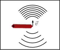
(a)

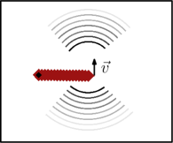
(b)

Figure 7. Different sound properties in the pendulum scenario. 7(a)) Depicts the Doppler effect. As the sound source moves near (away from) the observer, the arrival time of the emitted waves decreases (increases), thus increasing (decreasing) the frequency. 7(b)) Depicts the how the amplitude of the sound decreases with the distance from the source. Fading semi-circles denote smaller intensities.

4.1.2. Learn to act in the world

The agent learned how to perform the task using the DDPG algorithm, while only having access to the image input modality—that is $\boldsymbol{I}_{\mathrm{train}}=I_{\mathrm{image}}$. These image observations are encoded into the latent space using $\mathcal{F}_{\mathrm{train}}=\mathcal{F}_{\mathrm{image}}$—the image-specific encoder of the AVAE trained in 4.1.1. Thus, the agent learns a policy $\pi$ that maps latent states to actions.

The actor and critic networks consisted of two fully connected layers of $256$ neurons each. The replay buffer was initially filled with samples obtained using a controller based on the Ornstein-Uhlenbeck process, with the parameters suggested by Lillicrap et al. (2015). The Adam gradient was used for optimizing both networks, with learning rates $\eta_{\textsc{critic}}$ and $\eta_{\textsc{actor}}$.

4.1.3. Transfer policy

We evaluated the performance of the policy trained in 4.1.2, when the agent only has access to the sound input modality, i.e., $\boldsymbol{I}_{\mathrm{test}}=I_{\mathrm{sound}}$.

Given a sound observation, the agent first preprocesses it using the latent map $\mathcal{F}_{\mathrm{test}}=\mathcal{F}_{\mathrm{sound}}$, generating a multimodal latent state $\boldsymbol{z}$—we denote this process as avae_s. The agent then uses the policy to select the optimal action in this latent state.

As a result, we are measuring the zero-shot transfer performance of policy $\pi$—that is, the ability of the agent to perform its task while being provided perceptual information that is completely different from what it saw during the reinforcement learning step, without any further training. Table 1 summarizes the transfer performance in terms of average reward observations throughout an episode of $300$ frames. Our approach avae_s + ddpg is compared with two baselines:

• random baseline, which depicts the performance of an untrained agent. This effectively simulates the performance one would expect from a non-transferable policy trained over image inputs, and later tested over sound inputs.

• sound ddpg baseline, a DDPG agent trained directly over sound inputs (i.e. the sounds correspond to the states). Provides an estimate on the performance an agent trained directly over the test input modality may achieve.

From Table 1, we conclude our approach provides the agent with an out-of-box performance improvement of over $300\%$, when compared to the untrained agent (non-transferable policy). It is also interesting to observe that the difference in performance between our agent and sound ddpg seems small, supporting our empirical observation that the transfer policy succeeds very often in the task: swinging the pole up.

4.2. hyperhot

We consider the hyperhot scenario, a novel top-down shooter game scenario inspired by the space invaders Atari game, where the goal of the agent is to shoot the enemies above, while avoiding their bullets by moving left and right.

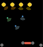
Figure 8. Visual and sound perceptual information in the hyperhot scenario. All enemies and bullets emit sounds that are received by four microphones at bottom left and right ($bl,br$) and paddle left and right ($pl,pr$).

Table 1. Zero-shot performance of the policy trained over the image input modality, when using sound inputs only. Presents the average reward per episode, over $75$ episodes. Results averaged over $10$ randomly seeded runs.

pendulum
	Rewards
Approach	avg ${\boldsymbol{\pm}}$ std
avaes + ddpg	$-2.00\pm 0.97$
random	$-6.30\pm 0.29$
sound ddpg	$-1.41\pm 0.91$

Similarly to the pendulum, in this scenario, the observations of the environment include both image and sound components. In hyperhot, however, the environmental sound is generated by multiple entities $e_{i}$ emitting a predefined frequency $f_{0}^{(i)}$:

• Left-side enemy units, $e_{0}$, and right-side enemy units, $e_{1}$, emit sounds with frequencies $f_{0}^{(0)}$ and $f_{0}^{(1)}$, respectively.

• Enemy bullets. $e_{2}$, emit sounds with frequency $f_{0}^{(2)}$.

• The agent’s bullets, $e_{3}$, emit sounds with frequency $f_{0}^{(3)}$.

The sounds produced by these entities are received by a set of $S$ sound receivers $\left\{\rho_{1},\dots,\rho_{S}\right\}$. Figure 8 depicts the scenario, where the yellow circles are the enemies; the green and blue bullets are friendly and enemy fire, respectively; the the agent is in red; and the sound receivers correspond to the white circles. The agent is rewarded for shooting the enemies, with the following reward function:

$$r=\begin{cases}10&\text{if all enemies are killed, \emph{i.e.}, win}\\ -1&\text{if player is killed or time is up, \emph{i.e.}, lose}\\ 0&\text{otherwise}\end{cases}$$

The environment resets whenever the agent collects a non-zero reward, be it due to winning or losing the game.

We assume the perceptual space of the agent as $\mathcal{I}=I_{\mathrm{image}}\times I_{\mathrm{sound}}$, with the visual input modality of the agent, $I_{\mathrm{vision}}$, consisting in the raw image observation of the environment. The sound, however, is generated in a more complex and realistic way. We model the sinusoidal wave of each sound-emitter $e_{i}$ considering its specific frequency $f_{0}^{(i)}$ and amplitude $a_{0}^{(i)}$. At every frame, we consider the sound waves of every emitter present in the screen, according to their distance to each sound receiver in $S$. The sound wave generated by emitter $e_{i}$ is observed by receiver $\rho_{j}$ as

$$a^{(i)}=a_{0}^{(i)}\exp{\left(-\delta\|\boldsymbol{e}_{i}-\boldsymbol{\rho}_{j}\|^{2}\right)}$$

where $\delta$ is a scaling constant, $\boldsymbol{e}_{i}$ and $\boldsymbol{\rho}_{j}$ denote the positions of sound emmitter $e_{i}$ and sound receiver $\rho_{j}$, respectively. We generate each sinusoidal sound wave for a total of $1047$ discrete time steps, considering an audio sample rate of $31\,400$ Hz and a video frame-rate of 30 fps. As such, each sinusoidal sound wave represents the sound heard for the duration of a single video-frame of the game. Finally, for each sound receiver, we sum all emitted waves and encode the amplitude values in 16-bit audio depth, considering a maximum amplitude value of $a_{M}$ and a minimum value of $-a_{M}$.

We now provide details on how our approach was set up. All constants and training hyper-parameters used are again summarized in Appendix A.1.

4.2.1. Learn a perceptual model of the world

We trained an AVAE model to learn the family of latent mapping $\mathcal{F}$, with a dataset $\mathcal{D}(\mathcal{I})$ with $M$ observations of images and sounds collected using a random controller. Before training, the images were preprocessed to black and white and resized to $80\times 80$ pixels, and the sounds normalized to the range $\left[0,1\right]$.

For the image-specific encoder we adopted an architecture with three convolutional layers and two fully connected layers. The three convolutional layers learned $32,64$ and $64$ filters, respectively. The filters were parameterized by kernel sizes $8,4$ and $2$; strides $4,2$ and $1$; and paddings $2,1$ and $1$. ReLU activations were used throughout. For the sound-specific component, we used two fully connected layers of $512$ neurons each, with one dimension batch normalization between the layers. The decoders followed similar architectures. The increase in size of these layers when compared to the pendulum task is due to more complex nature of the sounds considered in this scenario. The optimizer and loss function were configured in the same way as in the previous scenario.

4.2.2. Learn to act in the world

The agent learned how to play the game using the DQN algorithm, while having access only to image observations, $\boldsymbol{I}_{\mathrm{train}}=I_{\mathrm{image}}$, corresponding to the video game frames. The image observations are encoded into the latent space using $\mathcal{F}_{\mathrm{train}}=\mathcal{F}_{\mathrm{image}}$—the image-specific encoder of the AVAE model trained in the previous step. As such, the policy learned to play the game, maps these latent states to actions.

The policy and target networks consisted of two fully connected layers of $512$ neurons each, and we adopted a decaying $\epsilon$-greedy policy.

4.2.3. Transfer policy

We then evaluated the performance of the policy learned with image inputs, when the agent only has access to the sound modality, i.e., $\boldsymbol{I}_{\mathrm{test}}=I_{\mathrm{sound}}$. Given a sound observation, the agent preprocesses it using the latent map $\mathcal{F}_{\mathrm{test}}=\mathcal{F}_{\mathrm{sound}}$, thus generating a multimodal latent state $\boldsymbol{z}$—this process is denoted as avae_s. The agent then uses the policy to select the optimal action in this latent state.

Table 2 summarizes the transfer performance of the policy produced by our approach avae_s + dqn, in terms of average discounted rewards and game win rates over $100$ episodes. We compare the performance of our approach with additional baselines:

• avae_v + dqn, an agent similar to ours, but encodes the latent space with visual observations (as opposed to sounds).

• image dqn, a DQN agent trained directly over the visual inputs.

Considering the results in Table 2, we observe:

• A considerable performance improvement of our approach over the untrained agent. The average discounted reward of the random baseline is negative, meaning this agent tends to get shot often, and rather quickly. This is in contrast with the positive rewards achieved by our approach. Moreover, the win rates achieved by our approach surpass those of the untrained agent by $5$-fold.

• A performance comparable to that of the agent trained directly on the sound, sound dqn. In fact, the average discounted rewards achieved by our approach are slightly higher. However, we note that the sound dqn agent followed the same DQN architecture and number of training steps used in our approach. It is plausible that with further parameter tuning, the sound dqn agent could achieve better performances.

• The approach that could fine-tune to the most informative perceptual modality, image dqn, achieved the highest performances. Our approach, while achieving lower rewards, is the only able to perform cross-modality policy transfer, that is, being able to reuse a policy trained on a different modality. One may argue that this trade-off is worthwhile.

The DQN networks of all approaches followed similar architectures and were trained for the same number of iterations.

Table 2. Zero-shot performance of the policy trained over the image modality, when using sound inputs only. Provides a comparison with different baselines. Middle column is the average discounted reward per episode. Right column is the win rate of the agent. Both averaged over $100$ episodes. Results averaged over $10$ randomly seeded runs.

hyperhot
	Rewards	Win pct
Approach	avg $\pm$ std	avg $\pm$ std
avaes + dqn	$0.15$ p m 0.16	$36.1$ p m 10.38
avaev + dqn	$0.21$ p m 0.11	$43.20$ p m 7.03
random	$-0.33$ p m 0.16	$8.3$ p m 5.75
sound dqn	$0.1$ p m 0.22	$27.3$ p m 21.44
image dqn	$1.54$ p m 0.20	$75.00$ p m 5.33

4.3. Discussion

The experimental evaluation performed shows the efficacy and applicability of our approach. The results show that this approach effectively enables an agent to learn and exploit policies over different subsets of input modalities. This sets our work apart from existing ideas in the literature. For example, DARLA follows a similar three-stages architecture to allow RL agents to learn policies that are robust to some shifts in the original domains Higgins et al. (2017). However, that approach implicitly assumes that the source and target domains are characterized by similar inputs, such as raw observations of a camera. This is in contrast with our work, which allows agents to transfer policies across different input modalities.

Our approach achieves this by first learning a shared latent representation that captures the different input modalities. In our experimental evaluation, for this first step, we used the AVAE model, which approximates modality-specific latent representations, as discussed in Section 3.1. This model is well-suited to the scenarios considered, since these focused on the transfer of policies trained and reused over distinct input modalities. We envision other scenarios where training could potentially take into account multiple input modalities at the same time. Our approach supports these scenarios as well, when considering a generative model such as JMVAE Suzuki et al. (2016), which can learn joint modality distributions and encode/decode both modalities simultaneously.

Furthermore, our approach also supports scenarios where the agent has access to more than two input modalities. The AVAE model can be extended to approximate additional modalities, by introducing extra loss terms that compute the divergence of the new modality specific latent spaces. However, it may be beneficial to employ generative models specialized on larger number of modalities, such as the M²VAE Korthals (2019).

5. Conclusions

In this paper we explored the use of multimodal latent representations for capturing multiple input modalities, in order to allow agents to learn and reuse policies over different modalities. We were particularly motivated by scenarios of RL agents that learn visual policies to perform their tasks, and which afterwards, at test time, may only have access to sound inputs.

To this end, we formalized the multimodal transfer reinforcement learning problem, and contributed a three stages approach that effectively allows RL agents to learn robust policies over input modalities. The first step builds upon recent advances in multimodal variational autoencoders, to create a generalized latent space that captures the dependencies between the different input modalities of the agent, and allow for cross-modality inference. In the second step, the agent learns how to perform its task over this latent space. During this training step, the agent may only have access to a subset of input modalities, with the latent space being encoded accordingly. Finally, at test time, the agent may execute its task while having access to a possibly different subset of modalities.

We assessed the applicability and efficacy of our approach in different domains of increasing complexity. We extended well-known scenarios in the reinforcement learning literature to include, both the typical raw image observations, but also the novel sound components. The results show that the policies learned by our approach were robust to these different input modalities, effectively enabling reinforcement learning agents to play games in the dark.

Appendix A Appendix

A.1. Constants and hyper-parameters

	$f_{0}$	$440.0$Hz
	$K$	$1.0$
scenario	$c$	$20.0$
	sound receivers	$\left\{lb,rb,mt\right\}$
	frame stack	$2$
	latent space	$10$
	$\lambda_{\mathrm{image}},\lambda_{\mathrm{sound}},\beta,\alpha$	$1.0$
avae	batch size	128
	epochs	500
	$\eta_{\textsc{avae}}$	$1\mathrm{e}{-3}$
	$M$	$20\,000$
	batch size	128
	$\eta_{\textsc{actor}}$, $\eta_{\textsc{critic}}$	$1\mathrm{e}{-4}$, $1\mathrm{e}{-3}$
ddpg	$\gamma$	$0.99$
	max episode length	300 frames
	replay buffer	$25\,000$
	max frames	$150\,000$
	$\tau$	$1\mathrm{e}{-3}$

Table 3. Constants used in the pendulum scenario.

	$f_{0}^{0},\ f_{0}^{1},\ f_{0}^{2},\ f_{0}^{3}$	$(261,329,392,466)$ Hz
	$a_{0}^{0},\ a_{0}^{1},\ a_{0}^{2},\ a_{0}^{3},\ a_{M}$	$1.0$
scenario	$\delta$	$0.025$
	$c$	$20.0$
	sound receivers	$\left\{lb,rb,pl,pr\right\}$
	frame stack	$2$
	latent space	$40$
	$\lambda_{\mathrm{image}}$	$0.02$
	$\lambda_{\mathrm{sound}}$	$0.015$
	$\beta$	$1\mathrm{e}{-5}$
avae	$\alpha$	$0.05$
	batch size	128
	epochs	250
	$\eta_{\textsc{avae}}$	$1\mathrm{e}{-3}$
	$M$	$32\,000$
	batch size	128
	$\eta$	$1\mathrm{e}{-5}$
dqn	$\gamma$	$0.99$
	max episode length	450 frames
	replay buffer	$350\,000$
	max frames	$1\,750\,000$

Table 4. Constants used in hyperhot scenario.

References

- (1)
- Bellemare et al. (2013) Marc G. Bellemare, Yavar Naddaf, Joel Veness, and Michael Bowling. 2013. The Arcade Learning Environment: An Evaluation Platform for General Agents. Journal of Artificial Intelligence Research 47 (Jun 2013), 253—279.
- Brockman et al. (2016) Greg Brockman, Vicki Cheung, Ludwig Pettersson, Jonas Schneider, John Schulman, Jie Tang, and Wojciech Zaremba. 2016. OpenAI Gym. (2016). arXiv:cs.LG/1606.01540
- Damasio (1989) Antonion R. Damasio. 1989. Time-locked multiregional retroactivation: A systems-level proposal for the neural substrates of recall and recognition. Cognition 33, 1-2 (1989), 25–62.
- Finn et al. (2016) Chelsea Finn, Xin Yu Tan, Yan Duan, Trevor Darrell, Sergey Levine, and Pieter Abbeel. 2016. Deep spatial autoencoders for visuomotor learning. In 2016 IEEE International Conference on Robotics and Automation (ICRA). IEEE, 512–519.
- Gelada et al. (2019) Carles Gelada, Saurabh Kumar, Jacob Buckman, Ofir Nachum, and Marc G. Bellemare. 2019. DeepMDP: Learning Continuous Latent Space Models for Representation Learning. (2019). arXiv:cs.LG/1906.02736
- Higgins et al. (2017) Irina Higgins, Arka Pal, Andrei Rusu, Loic Matthey, Christopher Burgess, Alexander Pritzel, Matthew Botvinick, Charles Blundell, and Alexander Lerchner. 2017. DARLA: Improving Zero-Shot Transfer in Reinforcement Learning. In Proceedings of the 34th International Conference on Machine Learning (Proceedings of Machine Learning Research), Vol. 70. PMLR, 1480–1490.
- Kingma and Welling (2013) Diederik P. Kingma and Max Welling. 2013. Auto-Encoding Variational Bayes. (2013). arXiv:stat.ML/1312.6114
- Korthals (2019) Timo Korthals. 2019. M2VAE - Derivation of a Multi-Modal Variational Autoencoder Objective from the Marginal Joint Log-Likelihood. (2019). arXiv:cs.LG/1903.07303
- Lillicrap et al. (2015) Timothy P. Lillicrap, Jonathan J. Hunt, Alexander Pritzel, Nicolas Heess, Tom Erez, Yuval Tassa, David Silver, and Daan Wierstra. 2015. Continuous control with deep reinforcement learning. (2015). arXiv:cs.LG/1509.02971
- Meyer and Damasio (2009) Kaspar Meyer and Antonio Damasio. 2009. Convergence and divergence in a neural architecture for recognition and memory. Trends in Neurosciences 32, 7 (2009), 376–382.
- Mnih et al. (2015) Volodymyr Mnih, Koray Kavukcuoglu, David Silver, Andrei A Rusu, Joel Veness, Marc G Bellemare, Alex Graves, Martin Riedmiller, Andreas K Fidjeland, Georg Ostrovski, et al. 2015. Human-level control through deep reinforcement learning. Nature 518, 7540 (2015), 529.
- Ramachandran et al. (2017) Prajit Ramachandran, Barret Zoph, and Quoc V. Le. 2017. Searching for Activation Functions. (2017). arXiv:cs.NE/1710.05941
- Rezende et al. (2014) Danilo Jimenez Rezende, Shakir Mohamed, and Daan Wierstra. 2014. Stochastic Backpropagation and Approximate Inference in Deep Generative Models. (2014). arXiv:stat.ML/1401.4082
- Sutton and Barto (1998) Richard Sutton and Andrew Barto. 1998. Reinforcement Learning: An Introduction. MIT press Cambridge.
- Suzuki et al. (2016) Masahiro Suzuki, Kotaro Nakayama, and Yutaka Matsuo. 2016. Joint Multimodal Learning with Deep Generative Models. (2016). arXiv:stat.ML/1611.01891
- Watkins (1989) Christopher Watkins. 1989. Learning from delayed rewards. Ph.D. Dissertation. Cambridge University.
- Yin et al. (2017) Hang Yin, Francisco S. Melo, Aude Billard, and Ana Paiva. 2017. Associate Latent Encodings in Learning from Demonstrations. In Proceedings of the Thirty-First AAAI Conference on Artificial Intelligence (AAAI’17). AAAI Press, 3848–3854.
- Zhang et al. (2018) Marvin Zhang, Sharad Vikram, Laura Smith, Pieter Abbeel, Matthew J. Johnson, and Sergey Levine. 2018. SOLAR: Deep Structured Representations for Model-Based Reinforcement Learning. (2018). arXiv:cs.LG/1808.09105