How weakened cold pools open for convective self-aggregation

Abstract

In radiative-convective equilibrium (RCE) simulations, convective self-aggregation (CSA) is the spontaneous organization into segregated cloudy and cloud-free regions. Evidence exists for how CSA is stabilized, but how it arises favorably on large domains is not settled. Using large-eddy simulations (LES), we link the spatial organization emerging from the interaction of cold pools (CPs) to CSA. We systematically weaken simulated rain evaporation to reduce maximal CP radii, $R_{\text{max}}$, and find reducing $R_{\text{max}}$ causes CSA to occur earlier. We further identify a typical rain cell generation time and a minimum radius, $R_{\text{min}}$, around a given rain cell, within which the formation of subsequent rain cells is suppressed. Incorporating $R_{\text{min}}$ and $R_{\text{max}}$, we propose a toy model that captures how CSA arises earlier on large domains: when two CPs of radii $r_{i,j}\in[R_{\text{min}},R_{\text{max}}]$ collide, they form a new convective event. These findings imply that interactions between CPs may explain the initial stages of CSA.

I Key Points

1. Smaller cold pool radii in large-eddy simulations (LES) diminishes the time to reach convective self-aggregation.

2. Incorporating the maximal cold pool radius and the radius of suppressed regions into a simple model gives realistic self-aggregation.

3. The model supports the role of cold pools and captures the effect of domain size, where larger domain size facilitates self-aggregation.

II Plain Language Summary

Convective self-aggregation (CSA) describes the emergence of persistently dry, cloud-free areas in numerical simulations. It has been suggested as a possible mechanism for tropical cyclone formation and large-scale events such as the Madden-Julian Oscillation. Some understanding of the persistence of CSA exists. However, how CSA initially emerges remains poorly understood. Recently, the dynamics of cold pools (CPs) have been associated with the organization of convective events. CPs are radially expanding pockets of dense air that form under precipitating thunderstorms. In this work, we ask how weakening CPs could facilitate the emergence of CSA. By analyzing high-resolution numerical simulations, we show that reducing rain evaporation shortens the time before CSA sets in. These simulations demonstrate that CPs reach greater radii when rain evaporation is large. In addition, we find that new convective events occur near the point where two CPs collide. Finally, we find a minimum CP radius within which CPs are too negatively buoyant to initialize new convective events. Building on these numerical findings, we propose a simple idealized mathematical model that approximates CPs as expanding and colliding circles. We show that this model can capture the emergence of CSA. We conclude that the lack of CPs facilitates CSA.

III Introduction

When evaporation of rain from convective clouds is strong, so is the associated sub-cloud cooling and density increase Simpson [1980], Engerer et al. [2008], forcing the resulting cold pools (CPs) to spread more quickly and cover larger areas Romps and Jeevanjee [2016], Torri et al. [2015], Zuidema et al. [2017]. Such pronounced CP activity has repeatedly been suggested to hamper convective self-aggregation (CSA) in radiative-convective equilibrium (RCE) numerical experiments Jeevanjee and Romps [2013], Muller and Bony [2015], Holloway and Woolnough [2016], Hohenegger and Stevens [2016], Yanase et al. [2020]. In these simulations, the atmosphere gradually organizes from an initial homogeneous population of convective updrafts into a segregated pattern with strongly convecting regions and dry, precipitation-free regions Held et al. [1993], Tompkins and Craig [1998], Bretherton et al. [2005], Hohenegger and Stevens [2016], Wing et al. [2017].

Generically, CSA is characterized by the appearance of long-lived dry and warm patches, within which rain is suppressed Holloway et al. [2017]. Further drying increasingly occurs through enhanced radiative cooling in already dry regions and the resulting subsidence. Later, the dry regions expand and merge, eventually leaving only one contiguous moist area with intense low-level convergence feeding convection. Surface latent and sensible heat fluxes — which increase under stronger surface wind speed — may further increase such low-level moisture convergence.

CPs are capable of mediating organization, as they effectively relay ”information” between one precipitating cloud and its surroundings. Physically, CPs spread as density currents along the surface, carry kinetic energy and buoyancy, and modify the thermodynamic structure near the CP edges Tompkins [2001], Langhans and Romps [2015], de Szoeke et al. [2017]. CPs thereby act to pattern the convectively unstable atmosphere, establishing connections between the loci where new convective cells emerge and loci at which the previous cells dissipated. In particular, new cells were suggested to be spawned by the CP gust front alone or by collisions between mobile gust fronts de Szoeke et al. [2017], Glassmeier and Feingold [2017], Cafaro and Rooney [2018], Fuglestvedt and Haerter [2020]. Inspired by the notion of CP interactions, conceptual work has formulated CPs as cellular automata Böing [2016], Windmiller [2017], Haerter et al. [2019, 2020], and CP representations have been incorporated into large-scale models Grandpeix and Lafore [2010].

Studies on convective self-aggregation often argue that sufficiently large domain size is required for the phenomenon to emerge Bretherton et al. [2005], Muller and Bony [2015], especially when the horizontal resolution is coarse, e.g., at least 500 km for resolutions finer than 2 km Yanase et al. [2020]. To examine this claim more closely, for deliberately small domain sizes and fine horizontal resolution, we here show that CSA sets in earlier when CPs are weakened through reductions in rain evaporation — that is, when the CP maximal radius, termed $R_{\text{max}}$, is reduced. We track the CP gust fronts to motivate that loci of gust front collisions are preferable for subsequent convective rain cells — hence, that CP interactions are essential in organizing the precipitation field. Dependent on rain evaporation, we further detect a minimal distance $R_{\text{min}}$, within which subsequent rain cells are unlikely to form, as well as a typical generation time. Using these findings, we build, simulate, and analyze a simple mathematical model, which helps understand cloud-free regions’ formation. We explore the phase diagram of this model and find that, when initialized at a high density of rain cells, the population of subsequent rain cells will either remain high or transition to a low state with only a subregion covered by rain cells. The change from high to low density occurs later for large $R_{\text{max}}$ or small domain sizes $L$.

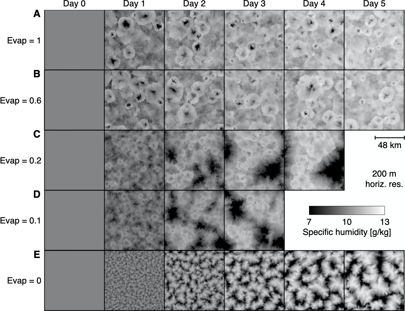
Figure 1: The onset of convective self-aggregation. Near-surface specific humidity $q_{v}$(50 m) the first 10 min of each simulation day in RCE simulations with various degrees of rain evaporation. (A) Realistic rain evaporation (control simulation). (B) 60%, (C) 20%, (D) 10%, and (E) 0% rain evaporation relative to (A). Within cold pool centers, note the pronounced moisture reduction in (A–B) and the weakened moisture reduction in (C–D). Besides, note the evolving moisture segregation, which is typical of convective self-aggregation (C–D) and moisture coarsening progression (E).

IV Materials and Methods

Large-eddy simulations. We carried out (96 km)² simulations of the convective atmosphere for up to five simulation days using the University of California, Los Angeles (UCLA) Large Eddy Simulator with sub-grid scale turbulence parametrized after Smagorinsky Smagorinsky [1963]. We combine with a delta four-stream radiation Pincus and Stevens [2009] and a two-moment cloud microphysics scheme Stevens et al. [2005]. Rain evaporation is accounted for by Seifert and Beheng (2006). All five simulations are identical, except that rain evaporation is varied within fractions $\{0,.1,.2,.6,1.0\}$ of its default. In the following, the corresponding simulations are labeled ”Evap=0”, ”Evap=0.1”, etc. We reduce computed rain evaporation by the corresponding factor — hence, less hydrometeor mass is converted to water vapor. Surface temperatures are set constant to 300 K, and insolation is fixed using a constant equatorial zenith angle of 50^∘ (constant 655 W m^-2) Bretherton et al. [2005]. Surface heat fluxes are computed interactively and depend on the vertical temperature and humidity gradients and horizontal wind speed, which is approximated using the Monin-Obukhov similarity theory. Temperature and humidity are initialized using a prior approximately 3-day spin-up using 400 m horizontal resolution (see Fig. S1). The horizontal model grid is regular, and periodic boundary conditions are applied in both lateral dimensions. Vertically, the model resolution varies from 100 m below 1 km, stretching to 200 m near 6 km and finally 400 m in the upper layers. There are 75 vertical levels. The Coriolis force and the mean wind were set to zero with weak random initial perturbations added as noise to break complete spatial symmetry. At each output time step of 10 min, instantaneous surface precipitation intensity, specific humidity, temperature, liquid water mixing ratio, outgoing long-wave radiation, and 3D velocities are output at various model levels. To explore resolution effects, we supplemented the simulations described above using Evap=1 by otherwise similar simulations at 1km, 2km, and 4km horizontal resolution, each using $480\times 480$ horizontal grid boxes.

Tracking of cold pools. Cold pool (CP) gust fronts are tracked using tracer particles Haerter et al. [2019], Henneberg et al. [2020]. In any given time step, a sufficient number of tracers, $n_{tr}$, are placed at the edges (8-neighborhood) of an existing surface precipitation patch, which is a spatially contiguous area of rainy pixels (intensity $I>I_{0}$, with $I_{0}\equiv$ .5 mm h^-1). The first tracers are placed when the patch is first detected, and this time defines the time origin for each CP ($t$ = 0 in Fig. 2B). If the number of tracers placed is less than a maximal number $n_{tr,max}\equiv$ 100, i.e., $n_{tr}<n_{tr,max}$, then further tracers are placed at the patch edges during the subsequent timesteps until $n_{tr,max}$ is reached. If the rain patch disappears before $n_{tr,max}$ is reached, fewer tracers are used for that CP. This procedure was found sufficient in reliably tracking the gust fronts. Using a simple Euler method, the tracer particles are advected along with the radial velocity component in the lowest model level ($z$ = 50 m) and reliably settle in the gust fronts surrounding each CP. As this tracking method is implemented to run ”offline,” it uses only the recorded discrete 10 min output time steps. In the initial stages of tracking each CP, this sometimes leads to particles having to ”catch up” with the gust front (see Fig. 2A, for examples of such CPs). However, it is found that tracers consistently settle in the gust front after few time steps due to the strong radial velocity gradient. To transparently compare CP radii between the different simulations, which differ in time of rainfall onset (Fig. 2B), we first determine the time of onset for each simulation, that is, the time when the first surface rain patch with $I>I_{0}$ occurred. We then track all CP gust fronts during 1100 min. This interval was found sufficient to yield significant statistics on the spreading of each CP, but short enough so that not many CP collisions were encountered. Conversely, to study collision effects (Fig. 3), we used a late-stage ($\sim$ 4 days after initialization) of the realistic simulation (Evap=1). As CPs are space-filling, any new CP inevitably collides with recent CPs in its surroundings.

Mathematical model. We initialize $N_{1}=L^{2}/(10R_{\text{min}}^{2})$ points — the subscript indicates ”generation one” — at random locations selected uniformly on a 2D domain of size $L\times L$ with double-periodic boundary conditions. All points grow into circles representing CPs with equal and constant radial speed. The expanding circles have centers at $\overline{c}_{i}=[x_{i},y_{i}]$ and increasing radii $r_{i}$. At the collision point, [$x,y$], of two circles belonging to the same generation $g$ and having radii $r_{i}$ and $r_{j}$, a new expanding circle belonging to the subsequent generation $g+1$ emerges only if $R_{\text{min}}<r_{i},r_{j}<R_{\text{max}}$. Hence, for two CPs to form a new circle, their centers’ separation distance needs to be greater than $2R_{\text{min}}$ and less than $2R_{\text{max}}$. Colliding circles continue expanding, and new circles start growing instantaneously; hence, all circles, at all times, expand with equal and constant speed.

We find the collision point by solving $(x-x_{i})^{2}+(y-y_{i})^{2}=(r_{i}+dr)^{2}$ and $(x-x_{j})^{2}+(y-y_{j})^{2}=(r_{j}+dr)^{2}$, where $dr$ is the distance from the two circles’ rims to the collision point. Only collisions that fall onto the straight line between the two circle centers are allowed since that is the collision point with the highest momentum, yielding $y=\frac{x-x_{i}}{x_{j}-x_{i}}(y_{j}-y_{i})+y_{i}\,.$ These three quadratic equations have three unknowns ($x,y,dr$), and two solutions. One of these two solutions can be ruled out because only the positive real solution is relevant to this model.

Similar to the analytical approach in Haerter et al. [2019], we do not run the model strictly chronologically. To reduce simulation time, we take advantage of the fact that circles belonging to different generations cannot interact since they grow with equal and constant speed. Thereby, we calculate all collision points for each generation before proceeding to the next generation. Generally, the last circle in any generation will initiate later than the next generation’s first circle. Therefore, when moving to the next generation, we return to the time when the first circle of that generation was seeded.

The list of potential collision points is calculated for each generation and sorted incrementally by $dr$. We update the system by inserting circles at the collision points if $R_{\text{min}}<r_{i},r_{j}<R_{\text{max}}$, and if the subsequent generation does not occupy the collision point. This process is simulated until circle generation number 500 is reached.

V Results

Weakening cold pools in RCE simulations speeds up the onset of self-aggregation. A control simulation with realistic rain evaporation (Fig. 1A) shows no indication of CSA. We check this by computing the inter-quartile specific humidity difference (Fig. S2A), finding a weak initial increase when first CPs set in but no further increase over time. While leaving the total number of rain cells and domain-average rainfall approximately unchanged (Figs. S2B and S3), decreasing the rate of rain evaporation (Fig. 1B–E) yields a monotonic increase in humidity variation (Fig. S2A) and overall higher near-surface temperature (Fig. S2C), along with a systematically earlier onset of persistent dry patches, e.g., near day 2 for Evap=0.2 (Fig. 1C). This comparison underlines findings from Jeevanjee and Romps [2013] and Muller and Bony [2015], who reported that CPs hamper self-aggregation. The five experiments highlight that reducing rain evaporation weakens subsidence drying in the center of CPs (compare dark spots in Fig. 1A–B vs. C–D) and visibly reduces CP radii. We also note that intermediate values of evaporation appear to allow for a band-like aggregation state, where rain cells form a quasi-one-dimensional chain around one of the horizontal dimensions (Fig. 1C on day 4). When rain evaporation is entirely removed (Fig. 1E), any organizing effect through CPs is absent: one is left with a coarsening process akin to reaction-diffusion dynamics, Windmiller and Hohenegger [2019] small impurities gradually merging into larger structures. The dominant feedback can be ascribed to the net warming in the troposphere induced by deep convective clouds, thus promoting further convective activity in existing precipitation cells’ surroundings.

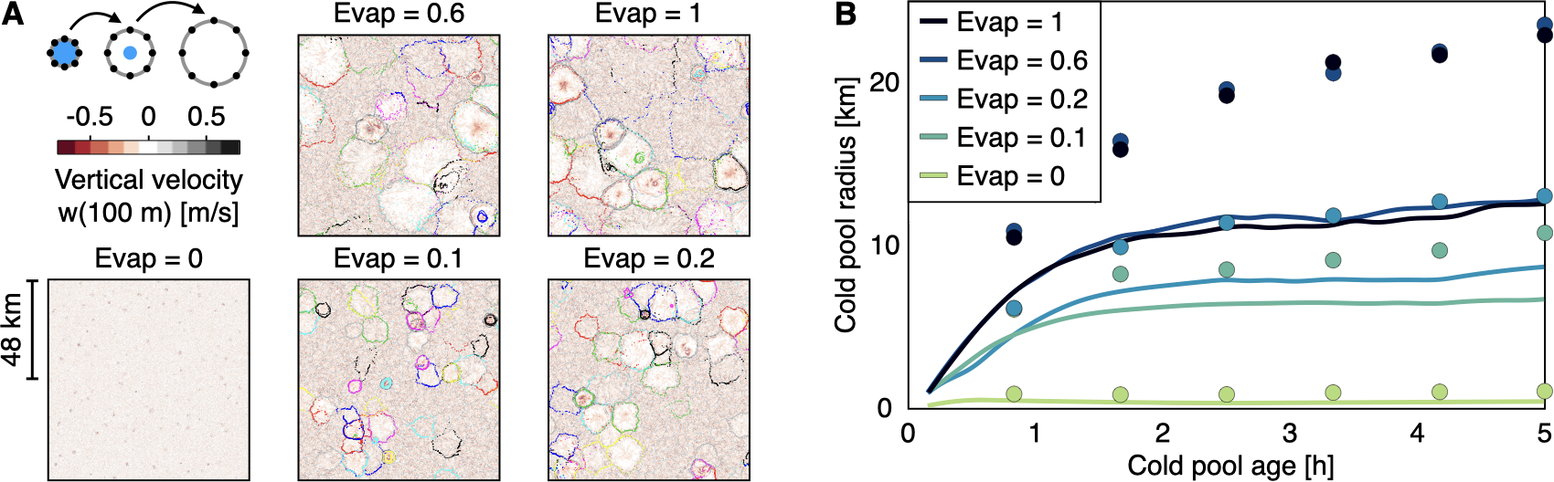
Figure 2: Maximum radius, $\mathbf{R_{max}}$. (A) Tracking all cold pool (CP) gust fronts from the onset of precipitation for 1,100 min. Top-left cartoon: we track a CP gust front (grey rim) by placing tracers (black points) around the rain event (blue spot) and let the tracers move radially away from the rain event with the horizontal wind (Details: Methods). Each panel shows the near-surface vertical velocity field at the end of the time interval and gust front tracers marked by colors indicating different CPs. (B) The average CP radii as the CPs evolve after their emergence (lines) and the 90th radius percentile (dots). Note that CPs initially grow quickly but monotonically slow and that maximal CP radii increase with rain evaporation rate.

Measuring cold pool radius. Using a rain cell Moseley et al. [2019] and CP Haerter et al. [2019], Henneberg et al. [2020] tracking method, we seed tracer particles at the boundary of surface rain patches (see cartoon in Fig. 2A). We advect these tracers using the radial velocity field, forcing them to gather in pronounced convergence areas caused by the CP gust fronts (Details: Methods). Superimposing the resulting pattern of tracers onto the near-surface vertical velocity field (Fig. 2A) shows that the tracers indeed gather along the edge of each CP (subsident or featureless vertical wind field). It is also visually apparent that radii systematically increase with the evaporation rate. The radius increase is confirmed by plotting the time evolution of the average CP radii in each simulation (Fig. 2B). For Evap=0, radii simply show the radii of the corresponding surface rain cells, as, without CPs, there is no pronounced wind field to advect the tracers. For Evap=1, CPs typically expand to $\approx$ 11 km a few hours after initiation, a value comparable to previous simulation results found on various domain sizes Romps and Jeevanjee [2016], Tompkins [2001] and observational findings Black [1978], Zuidema et al. [2012], Feng et al. [2015].

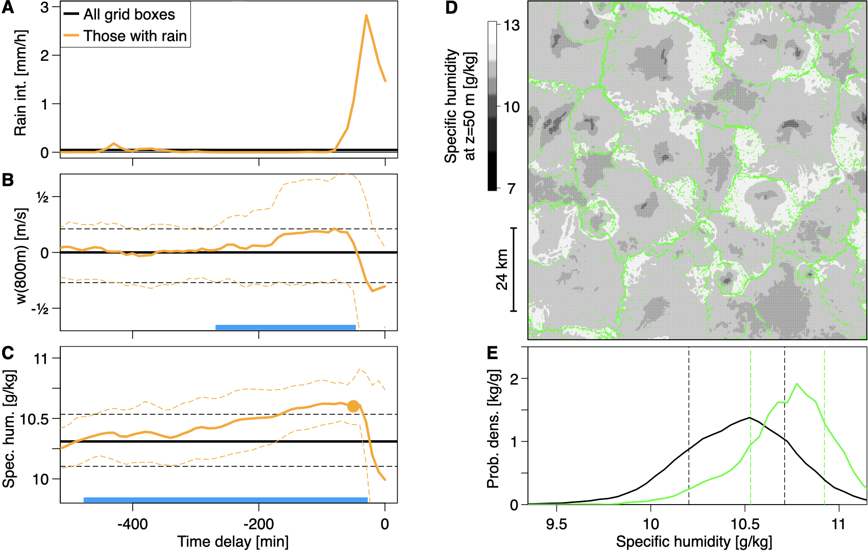
Figure 3: Identifying cold pool collisions. (A) Rain intensity conditionally averaged over all grid boxes with rainfall at $t$ = 0 (orange) and domain mean rainfall (black) for the simulation Evap=1. (B) Analog, but for vertical velocity near the cloud base ($w$(800 m)). The domain average is zero throughout. Thin lines mark corresponding 20th and 80th percentiles. Note the pronounced peak, corresponding to convective updrafts, as is expected before rain onset, as well as the dip near $t$ = 0, corresponding to CP associated downdrafts. (C) Analogous, but for near-surface specific humidity, $q_{v}$($z$ = 50 m). Note the relatively long buildup of humidity before rainfall onset. The blue bar highlights the time during which updrafts exceed the domain average. (D) Near-surface specific humidity field, $q_{v}$($z$ = 50 m). Tracer particles (green) visually lie at locations of CP gust fronts. The blue bar highlights the time during which specific humidity exceeds the domain average. (E) Histograms of $q_{v}$(50 m) for all data shown in panel D (black curve), and only the gust front positions (the green points in panel D).

New convective events are initiated in the vicinity of cold pool collisions. What is then the specific role of CPs in maintaining domain-wide convection? To explore this, first consider locations of rainfall at a particular time step of Evap=1 (Fig. 3A), the associated cloud-base vertical velocity (Fig. 3B), and specific humidity (Fig. 3C). Updrafts form shortly before the onset of rainfall, whereas specific humidity becomes elevated earlier — in line with the analysis of RCE simulations, where a considerable buoyancy build-up before any subsequent convective event was reported.Fuglestvedt and Haerter [2020] Second, we determine gust front loci using CP tracer particles Haerter et al. [2019], Henneberg et al. [2020] (Fig. 3D). Many of these tracers are located at the intersection between two CPs. It is visually apparent that such loci coincide with enhanced humidity (Fig. 3D). To quantify that tracers lie in regions of pronounced updrafts, we verified that the $q_{v}$(50 m)-histogram for all loci with tracers is shifted to markedly positive values (Fig. 3E). The histogram of peak humidity during rain event buildup (peak highlighted in Fig. 3C) shows a shift towards elevated values. Collecting, as a comparison, the specific humidity at CP gust fronts (Fig. 3E), it is found that this histogram is similarly shifted to moister values. In summary, loci of CP collisions do provide the positive humidity anomalies typical of subsequent convective events.

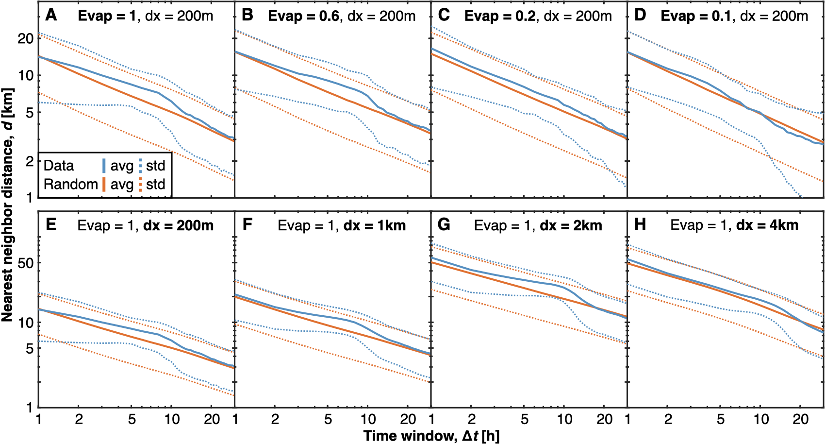
Figure 4: Generation time and an effective minimal radius, $\mathbf{R_{min}}$. (A–D) The average distance ($d$) between rain events occurring within the first 12h past precipitation onset and their nearest neighbor rain event (blue) occurring within a time window ($\Delta t$) for varying evaporation rates (Evap). We contrast that to a control where the same number of rain events are located randomly (red), given as the average distance $d$ of the probability density function $f(d)=2n\pi d(1-\pi d^{2}/L^{2})^{-1+n}/L^{2}$ where $L$ is the domain length and $n$ is the mean number of rain events during $\Delta t$. The dotted lines mark the standard deviations. More rain events are included for larger time windows, causing the distances to be smaller. In (A), note the lack of events within 5–6 km for up to 8h. (E–H) Analogous, but for varying horizontal resolutions ($dx$). Note the inhibitory distance increases for coarser resolutions without changing the time scale at which it occurs.

New deep convective events are initiated at a specific distance away from earlier events. To quantify a possible suppression effect caused by a present rain cell’s CP on subsequent cells forming within the surroundings, we examine whether rain events after the initial rain onset are spaced randomly or not. A non-random spacing would imply either suppression (larger distance) or activation (smaller distance), whereas a random spacing would speak against a direct spatial influence on subsequent rain cell formation. We thus identify all rain events within the first 12h after rain onset Moseley et al. [2013] allowing us to compare non-aggregating simulations with aggregating simulations (day 1 in Fig. 1). We measure each rain cell’s distance to it’s nearest rain event occurring within a time window $\Delta t$.

For the control simulation (Fig. 4A), we find an inhibitory effect causing the nearest neighbor distance to be $>5$ km for up to 8h. In contrast, it would linear decay on a log-log plot if events were distributed randomly in space (compare orange and blue curves in Fig. 4). We refer to this distance as $R_{\text{min}}\approx$ 6 km and explain it by CPs being too negatively buoyant to initialize new convective cells within this distance Drager and van den Heever [2017], Fournier and Haerter [2019]. When increasing the time window of included events from 8–12 hours, we find that this suppression effect disappears; that is, the distribution function matches the random one. On this time scale, the CPs associated with two rain events have time to grow larger than $R_{\text{min}}$, collide, and trigger the formation of a new, closer, rain event belonging to the subsequent generation. We, therefore, interpret this time scale as the generation time of one CP. We find this time scale unchanged across simulations, while the spatial scale increases for coarser horizontal resolutions (Fig. 4).

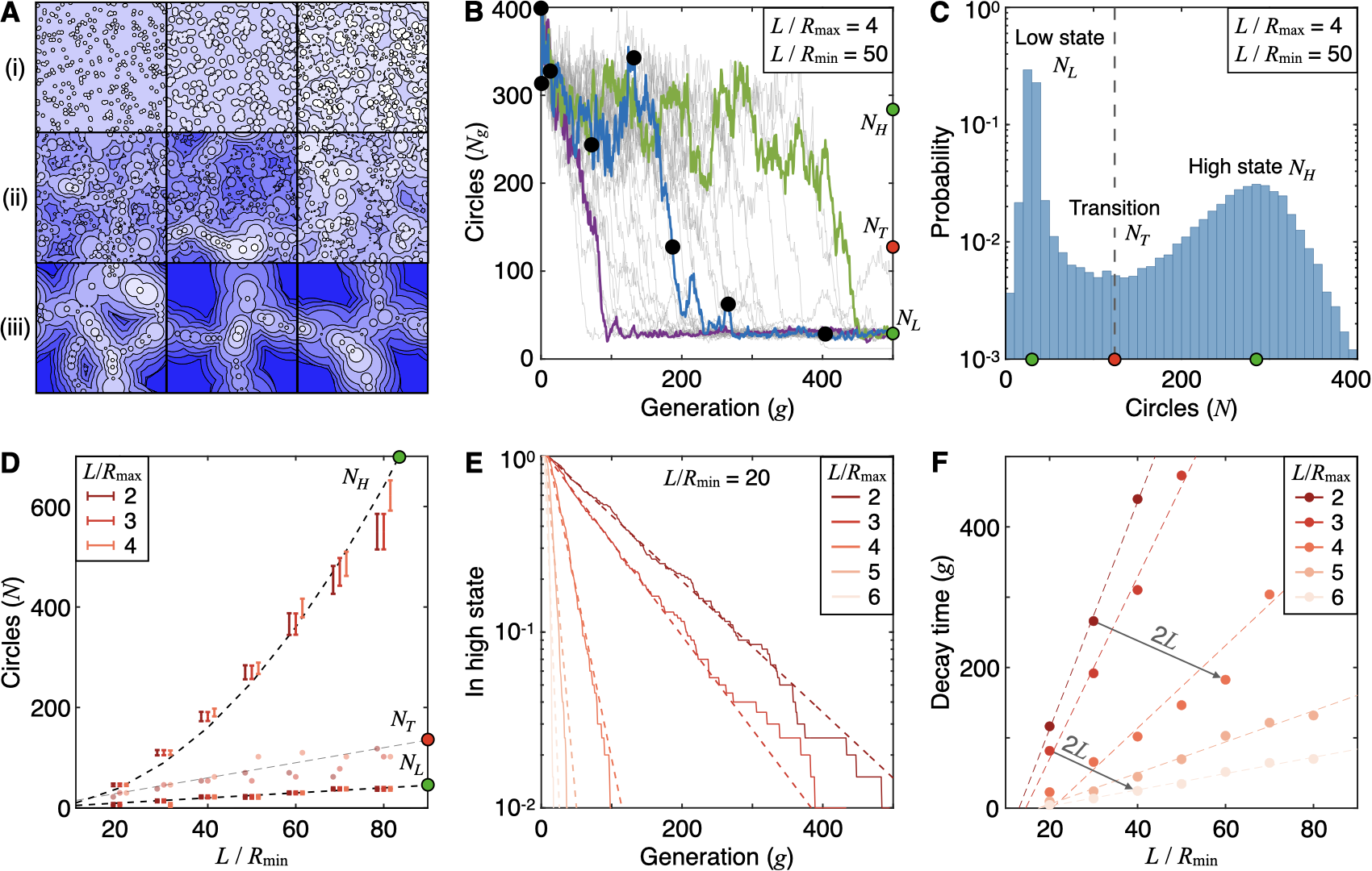
Figure 5: Circle model. (A) $N_{1}$ randomly located circles representing cold pools expand radially with equal and constant speed on an $L\times L$ domain. Any two colliding circles of radii $R_{\text{min}}<r_{i},r_{j}<R_{\text{max}}$ initiate a new expanding circle at their collision point (Details: Methods). Within each sub-panel, circles of the same color belong to the same generation and white (dark blue) areas correspond to the most recent (historic) generations in the respective sub-panel. (B) The number of circles ($N_{g}$) per generation ($g$) as 30 simulations evolve. Three runs are highlighted. The blue curve represents the simulation in (A), and the black dots indicate the snapshots’ time. Note the existence of two qualitatively distinct states of high and low $N_{g}$. (C) The distribution of circles in all generations pooled together for 200 runs. In (A–C), $L/R_{\text{min}}$ = 50 and $L/R_{\text{max}}$ = 4. In (B–D), the two green circles mark the low and the high states while the red circle marks the transition point. (D) The number of circles in the low $N_{L}$ and high $N_{H}$ states, and at the transition point $N_{T}$ for varying $L/R_{\text{max}}$ and $L/R_{\text{min}}$. (E) The fraction of runs in the high state as generation number for $L/R_{\text{min}}$ = 20. Note the logarithmic vertical axes. (F) The characteristic decay time as a function of $L/R_{\text{max}}$ and $L/R_{\text{min}}$. Note that higher $L$, higher $R_{\text{min}}$, or lower $R_{\text{max}}$ result in faster decay.

A simple mathematical model captures the onset of self-aggregation. To understand the role of CP collisions, we introduce a model consisting of growing and colliding circles. The circles represent the gust fronts of CPs and they are initialized uniformly at random inside the model domain. The circle radius, $r$, initially set to zero, increases linearly until $r=R_{\text{max}}$, hence the expansion velocity, $v(r)$, is a step function $v(r)=v_{0}\theta(R_{\text{max}}-r)$ where $v_{0}$ is a constant and $\theta(R_{\text{max}}-r)=1$ for $r<R_{\text{max}}$, otherwise $\theta=0$. After a given circle reaches $R_{\text{max}}$, it has no further effect and is removed. When two circles meet, both having their radii lie between $R_{\text{min}}$ and $R_{\text{max}}$, they instantly produce a new circle at the first point of intersection. The reasoning is that in RCE, most new rain cells result from thermodynamic pre-conditioning near the gust front collision lines (Fig. 3 and Fuglestvedt and Haerter, 2020), and the delay between the collision time and the initiation of the resultant rain cell is so large (typically several hours) that direct forced lifting can be ruled out. In line with the findings in Fig. 4, CPs with $r<R_{\text{min}}$ are considered too negatively buoyant to initialize new CPs Drager and van den Heever [2017], Fournier and Haerter [2019]. However, circles may collide with multiple other circles until they reach $R_{\text{max}}$ beyond which they have no role.

Mathematically, the collision dynamics allow us to categorize circles into generations: the initially seeded circles constitute generation one (panels 1–2 in Fig. 5A,i where all circles are smaller than $R_{\text{min}}$). Each collision is between circles belonging to the same generation $g$, and the resultant new circles belong to the subsequent generation $g+1$. $R_{\text{min}}>0$ prevents singularities, that is, infinitely rapid replication. Given $R_{\text{min}}=0$, an initial random generation-one population $N_{1}$ of circles would yield $N_{2}=2\,N_{1}$ (Details: Supplement), and subsequent growth of $N_{g}$ vs. $g$ would be nearly exponential. For $R_{\text{min}}>0$ circles must grow beyond $R_{\text{min}}$ and only then replicate to yield generation-two events (note the different color shadings in Fig. 5A,i, third panel). In Fig. 5A,ii new circles of various generations are initiated throughout the domain with no obvious patterning. However, during Fig. 5A,iii a separation into a circle-filled (convecting) and a circle-free (non-convecting) sub-region occurs. Note the visual similarity with the numerical experiment in Fig. 1C–D.

The number of circles $N_{g}$ in all simulations eventually drops from an initial high-$N$ state to one with low $N$ (Fig. 5B). The histogram of $N$, which is bimodal, confirms the notion of two distinct meta-stable states (Fig. 5C). Given this finding, we explore how the two states depend on the independent model parameters $L/R_{\text{min}}$ and $L/R_{\text{max}}$. We find that the low-$N$ state scales as $N_{L}=L/(2R_{\text{min}})$, whereas the high-$N$ state scales as $N_{H}=L^{2}/(10R_{\text{min}}^{2})$, both independent of $R_{\text{max}}$ (Fig. 5D). The transition point occurs at $N_{T}\approx 1.5L/R_{\text{min}}$ The linear scaling $N_{L}\sim L$ is commensurate with band-like, one-dimensional, structures (compare Fig. 5A,iii and Fig. 1C–D on day 2–4), whereas $N_{H}\sim L^{2}$ is in line with two-dimensional organization. By fitting the fraction of simulations in the high-$N$ state to an exponential function (Fig. 5E), we show that a characteristic time exists when the simulations decay to the low state. Thereby, we find that the circle model predicts decreasing $R_{\text{max}}$, increasing $L$, or increasing $R_{\text{min}}$ speed up the characteristic time when the transition occurs (Fig. 5F). Decreasing $R_{\text{max}}$ is in correspondence with the results presented in Figs. 1–2. Increasing $L$ has previously been reported to facilitate self-aggregation Bretherton et al. [2005], Muller and Bony [2015]. The literature also matches that coarser horizontal resolution favors self-aggregation given our result in Fig. 4E–H where we show that coarser horizontal resolution results in increased $R_{\text{min}}$ Hirt et al. [2020], Yanase et al. [2020].

VI Discussion and Conclusion

Convincing theories have been proposed for Turing-like coarsening of the RCE atmosphere into moist and dry sub-regions Bretherton et al. [2005], Craig and Mack [2013], Emanuel et al. [2014]. Such reaction-diffusion systems describe local positive feedback, e.g., of moisture on itself. In contrast, we here explicitly model the non-local, two-particle interaction resulting from interacting cold pool (CP) gust fronts — competing with the well-studied local moisture feedback. The notion that CP collisions form new convective events is well documented Purdom [1976], Weaver and Nelson [1982], Torri and Kuang [2019] and addressed in toy models Böing [2016], Haerter [2019]. Our study investigates how the CP radius influences CSA and builds on the finding that the total rain cell number is approximately constant across simulations (Fig. S3). Indeed, relatively constant rain cell numbers (Fig. S3) and rain intensities (Fig. S2B) are supported by radiation constraints on precipitation in RCE Held and Soden [2006]. Our circle model implicates that large CPs, as formed by pronounced rain evaporation, become space-filling where the whole domain is filled by CPs and there is a connected patch through the domain among CPs from the same generation. From hexagonal close-packing, a lower radius bound for space-filling would be $R_{\text{max}}>L(3\sqrt{3}N)^{-1/2}\approx 5.7\,km$, where $L=92\,km$ is the side length of the simulation domain and $N\approx 50$ is the number of CPs per generation (Fig. S3). For radii smaller than this, areas emerge that cannot be reached by newly initialized circles — a gap results, and the transition to CSA sets in. When (realistically) departing from perfect close-packing, the required value of $R_{\text{max}}$ may lie somewhat higher — commensurate with our findings (Fig. 2) and the transition to CSA between Evap=.6, where $R_{\text{max}}\approx$ 12 km, and Evap=.2, where $R_{\text{max}}\approx$ 8 km.

Our model simplifies CP expansion by assuming a step function $v(r)=v_{0}\theta(R_{\text{max}}-r)$. In reality, CPs initially grow quickly and their speed of spreading decreases gradually over the course of a few hours (Fig. 2B) Grant and van den Heever [2016, 2018]. Introducing a smoothly varying gust front speed into our model would require a time-dependent expansion speed factor and a numerically-approximate approach might then be more practicable Haerter et al. [2019]. The presented model further does not reach a final, fully-aggregated state, where a small fraction of the domain intensely convects indefinitely. This sustained activity might be obtained by adding spatial noise (displacing new circles slightly away from the exact geometric collision point) and systematically increased triggering probabilities for decreased overall rain area Haerter [2019]. Extensions could include explicit incorporation of the ”super-CP” Windmiller and Hohenegger [2019] and radiatively driven CP Coppin and Bony [2015], Yanase et al. [2020], constituting the two components of the final large-scale circulation. This model extension would allow triggering events at the edges of the intensely-convecting supercell due to convective CPs colliding with the opposing radiatively driven CP. Such circulation feedbacks may well be essential in stabilizing the final steady state but may not be required to develop the first dry patches and their initial growth, which we have focused on in this work.

Author Contributions

JOH ran and processed the large-eddy simulations, tracked the rain cells and cold pools, and contributed to the manuscript. SBN analyzed the simulation data, developed, implemented, analyzed the circle model, and drafted and revised the manuscript.

Competing Interests

The authors declare no competing interests.

How weakened cold pools open for convective self-aggregation

Silas Boye Nissen and Jan O. Haerter

Supplementary Information

Here, we analytically find the average number of circle collisions for neighbors in a system with randomly positioned cells, and we provide supplementary figures, including the initial conditions for the large-eddy simulations (Fig. S1), the time development of the domain-mean specific humidity variation, rain intensity, and temperature (Fig. S2), as well as the number of rainfall tracks (Fig. S3).

Direct circle collisions for random seeding. We seek to compute the number of direct circle collisions for an initial random population of circle centers, with circles emerging synchronously and at equal speed from all circle centers. By direct we mean, that the collision takes place along the line connecting the two circle centers involved. Finding the number of such collisions is equivalent to finding the number of line-of-sight connections (also known as a Gabriel connection) among these points (Fig. S4).

Consider $N$ points randomly seeded in a total area $A=\pi R^{2}$. A line-of-sight connection between any two points $\mathbf{r_{i}}$ and $\mathbf{r_{j}}$ at distance $l\equiv|\mathbf{r_{i}}-\mathbf{r_{j}}|$ exists if there are no points located inside the circle of radius $l/2$ centered at $(\mathbf{r_{i}}+\mathbf{r_{j}})/2$ (Fig. S4). This is the type of connection that we require for any two colliding circles to initialize the growth of a new circle in Fig. 5. One must further consider the probability of finding two points at distance $l$. For this purpose, define the density of points as $\rho\equiv N/A=N/\pi R^{2}$. Now consider the infinitesimal area $a(l)\equiv 2\pi\,l\,dl$ between two circles of radii $l$ and $l+dl$. The number of points contained in this area is

$$n(l)dl=\rho\,a(l)=\frac{2Nl}{R^{2}}dl.$$ (S1)

For any two points at a given distance $l$, we now consider the probability $p(l)$, that none of the remaining $N-2$ points lie within the circle of radius $l/2$:

$$P(l)=P_{0}^{N-2}=\left(1-\frac{\pi(l/2)^{2}}{\pi R^{2}}\right)^{N-2},$$ (S2)

where

$$P_{0}=1-\frac{\pi(l/2)^{2}}{\pi R^{2}}$$ (S3)

is the probability that any single point is not inside the area enclosed by a circle of radius $l/2$. Now the total number of expected line-of-sight (LOS) connections for a fixed given point to any of the other points can be computed:

$$N_{\text{LOS}} = \int_{0}^{R}dl\;n(l)P(l)$$ (S4)

$$= \int_{0}^{R}dl\frac{2Nl}{R^{2}}\left(1-\frac{l^{2}}{4R^{2}}\right)^{N-2}$$ (S5)

$$= \frac{4(1-\left(\frac{3}{4}\right)^{N-1})}{1-N^{-1}},$$ (S6)

which gives $\lim_{N\rightarrow\infty}N_{\text{LOS}}$ = 4. Hence, when repeating for all $N$ and avoiding double-counting of connections, one obtains that there are $2N$ line-of-sight connections when going from generation 1 to 2 for $R_{\text{min}}=0$ and $R_{\text{max}}=\infty$.

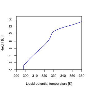
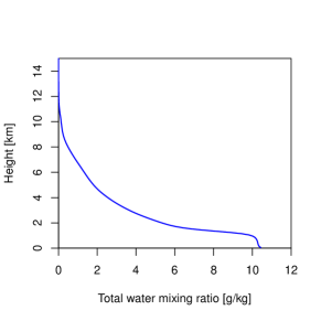
Figure S1: Initial condition. Vertical profiles for temperature (left) and moisture (right) used as the initial condition for all numerical experiments.

\begin{overpic}[trim=0.0pt 0.0pt 0.0pt 0.0pt,clip,width=130.08731pt]{dummy.pdf} \put(-83.0,0.0){\includegraphics[trim=0.0pt 0.0pt 0.0pt 0.0pt,clip,width=151.76964pt]{ q_timeseries_max-min}} \put(-4.0,0.0){\includegraphics[width=151.76964pt]{r_int_timeseries_only_rainevap.pdf}} \put(75.0,0.0){\includegraphics[width=151.76964pt]{T_timeseries_only_rainevap.pdf}} \put(-83.0,70.0){\large\bf A} \put(-4.0,70.0){\large\bf B} \put(75.0,70.0){\large\bf C} \end{overpic}

Figure S2: Humidity variation, domain mean rainfall, and temperature. (A) Each curve (see legend for line-style) was computed from the difference $\Delta q(t)\equiv q_{v,75}(t)-q_{v,25}(t)$, where the subscript numbers denote the respective percentiles of the specific humidity for each simulation and the argument $t$ denotes the specific simulation output time step. The continued increase for Evap $\in\{0,.1,.2\}$ signals the onset of self-aggregation for those cases. (B) Domain-mean rainfall for each simulation over time. (C) Domain-mean temperature for each simulation over time. We attribute the kink for the dis-aggregated simulations (Evap=.6 and Evap=1) near $t$ = .5 day to the onset of rainfall.

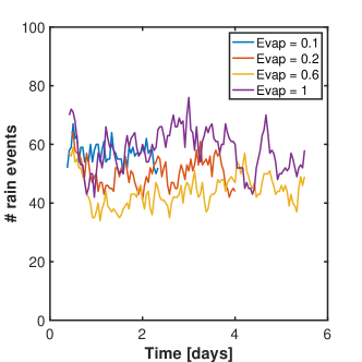
Figure S3: Timeseries of the number of rainfall tracks. Track counts were computed within a 6-hour running time window.

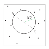
Figure S4: A line-of-sight connection. Schematic illustrating points in a 2D domain. Two points, ${\mathbf{r}_{i}}$ and ${\mathbf{r}_{j}}$, separated by a distance $l$ have a line-of-sight connection given that no points are located inside the circle of radius $l/2$ with the two points on its rim. In mathematics, this concept is also known as Gabriel neighbors.

References

- Simpson [1980] Joanne Simpson. Downdrafts as linkages in dynamic cumulus seeding effects. Journal of Applied Meteorology, 19(4):477–487, 1980.
- Engerer et al. [2008] Nicholas A Engerer, David J Stensrud, and Michael C Coniglio. Surface characteristics of observed cold pools. Monthly Weather Review, 136(12):4839–4849, 2008. doi: https://doi.org/10.1175/2008MWR2528.1.
- Romps and Jeevanjee [2016] David M Romps and Nadir Jeevanjee. On the sizes and lifetimes of cold pools. Quarterly Journal of the Royal Meteorological Society, 142(696):1517–1527, 2016. doi: https://doi.org/10.1002/qj.2754.
- Torri et al. [2015] Giuseppe Torri, Zhiming Kuang, and Yang Tian. Mechanisms for convection triggering by cold pools. Geophysical Research Letters, 42(6):1943–1950, 2015. doi: https://doi.org/10.1002/2015GL063227.
- Zuidema et al. [2017] Paquita Zuidema, Giuseppe Torri, Caroline Muller, and Arunchandra Chandra. A survey of precipitation-induced atmospheric cold pools over oceans and their interactions with the larger-scale environment. Surveys in Geophysics, pages 1–23, 2017. doi: https://doi.org/10.1007/s10712-017-9447-x.
- Jeevanjee and Romps [2013] Nadir Jeevanjee and David M Romps. Convective self-aggregation, cold pools, and domain size. Geophysical Research Letters, 40(5):994–998, 2013. doi: https://doi.org/10.1002/grl.50204.
- Muller and Bony [2015] Caroline Muller and Sandrine Bony. What favors convective aggregation and why? Geophysical Research Letters, 42(13):5626–5634, 2015. doi: https://doi.org/10.1002/2015GL064260.
- Holloway and Woolnough [2016] Chris E Holloway and Steven J Woolnough. The sensitivity of convective aggregation to diabatic processes in idealized radiative-convective equilibrium simulations. Journal of Advances in Modeling Earth Systems, 8(1):166–195, 2016. doi: https://doi.org/10.1002/2015MS000511.
- Hohenegger and Stevens [2016] Cathy Hohenegger and Bjorn Stevens. Coupled radiative convective equilibrium simulations with explicit and parameterized convection. Journal of Advances in Modeling Earth Systems, 8(3):1468–1482, 2016. doi: https://doi.org/10.1002/2016MS000666.
- Yanase et al. [2020] Tomoro Yanase, Seiya Nishizawa, Hiroaki Miura, Tetsuya Takemi, and Hirofumi Tomita. New critical length for the onset of self-aggregation of moist convection. Geophysical Research Letters, 47(16):e2020GL088763, 2020. doi: https://doi.org/10.1029/2020GL088763.
- Held et al. [1993] Isaac M Held, Richard S Hemler, and V Ramaswamy. Radiative-convective equilibrium with explicit two-dimensional moist convection. Journal of the Atmospheric Sciences, 50(23):3909–3927, 1993.
- Tompkins and Craig [1998] Adrian M Tompkins and George C Craig. Radiative–convective equilibrium in a three-dimensional cloud-ensemble model. Quarterly Journal of the Royal Meteorological Society, 124(550):2073–2097, 1998. doi: https://doi.org/10.1002/qj.49712455013.
- Bretherton et al. [2005] Christopher S Bretherton, Peter N Blossey, and Marat Khairoutdinov. An energy-balance analysis of deep convective self-aggregation above uniform SST. Journal of the Atmospheric Sciences, 62(12):4273–4292, 2005. doi: https://doi.org/10.1175/JAS3614.1.
- Wing et al. [2017] Allison A Wing, Kerry Emanuel, Christopher E Holloway, and Caroline Muller. Convective self-aggregation in numerical simulations: a review. Surveys in Geophysics, 38(6):1173–1197, 2017. doi: https://doi.org/10.1007/s10712-017-9408-4.
- Holloway et al. [2017] Christopher E Holloway, Allison A Wing, Sandrine Bony, Caroline Muller, Hirohiko Masunaga, Tristan S L’Ecuyer, David D Turner, and Paquita Zuidema. Observing convective aggregation. Surveys in Geophysics, 38(6):1199–1236, 2017. doi: https://doi.org/10.1007/s10712-017-9419-1.
- Tompkins [2001] Adrian M Tompkins. Organization of Tropical Convection in Low Vertical Wind Shears: The Role of Cold Pools. Journal of the Atmospheric Sciences, 58(13):1650–1672, 2001.
- Langhans and Romps [2015] Wolfgang Langhans and David M Romps. The origin of water vapor rings in tropical oceanic cold pools. Geophysical Research Letters, 42(18):7825–7834, 2015. doi: https://doi.org/10.1002/2015GL065623.
- de Szoeke et al. [2017] Simon P de Szoeke, Eric D Skyllingstad, Paquita Zuidema, and Arunchandra S Chandra. Cold pools and their influence on the tropical marine boundary layer. Journal of the Atmospheric Sciences, 74(4):1149–1168, 2017. doi: https://doi.org/10.1175/JAS-D-16-0264.1.
- Glassmeier and Feingold [2017] Franziska Glassmeier and Graham Feingold. Network approach to patterns in stratocumulus clouds. Proceedings of the National Academy of Sciences, 114(40):10578–10583, 2017. doi: https://doi.org/10.1073/pnas.1706495114.
- Cafaro and Rooney [2018] Carlo Cafaro and Gabriel G Rooney. Characteristics of colliding density currents: A numerical and theoretical study. Quarterly Journal of the Royal Meteorological Society, 144(715):1761–1771, 2018. doi: https://doi.org/10.1002/qj.3337.
- Fuglestvedt and Haerter [2020] Herman F. Fuglestvedt and Jan O. Haerter. Cold Pools as Conveyor Belts of Moisture. Geophysical Research Letters, 47(12):1–11, 2020. doi: https://doi.org/10.1029/2020GL087319.
- Böing [2016] Steven J Böing. An object-based model for convective cold pool dynamics. Mathematics of Climate and Weather Forecasting, 2(1), 2016. doi: https://doi.org/10.1515/mcwf-2016-0003.
- Windmiller [2017] Julia Miriam Windmiller. Organization of tropical convection. PhD thesis, Ludwig-Maximilian University, Munich, Germany, 2017.
- Haerter et al. [2019] Jan O Haerter, Steven J Böing, Olga Henneberg, and Silas Boye Nissen. Circling in on convective organization. Geophysical Research Letters, 46(12):7024–7034, 2019. doi: https://doi.org/10.1029/2019GL082092.
- Haerter et al. [2020] Jan O Haerter, Bettina Meyer, and Silas Boye Nissen. Diurnal self-aggregation. npj Climate and Atmospheric Science, 3(30):1–11, 2020. doi: https://doi.org/10.1038/s41612-020-00132-z.
- Grandpeix and Lafore [2010] Jean-Yves Grandpeix and Jean-Philippe Lafore. A density current parameterization coupled with Emanuel’s convection scheme. Part I: The models. Journal of the Atmospheric Sciences, 67(4):881–897, 2010. doi: https://doi.org/10.1175/2009JAS3044.1.
- Smagorinsky [1963] Joseph Smagorinsky. General circulation experiments with the primitive equations: I. the basic experiment. Monthly weather review, 91(3):99–164, 1963.
- Pincus and Stevens [2009] Robert Pincus and Bjorn Stevens. Monte Carlo spectral integration: A consistent approximation for radiative transfer in large eddy simulations. Journal of Advances in Modeling Earth Systems, 1(2):1–9, 2009. doi: https://doi.org/10.3894/JAMES.2009.1.1.
- Stevens et al. [2005] Bjorn Stevens, Chin-Hoh Moeng, Andrew S Ackerman, Christopher S Bretherton, Andreas Chlond, Stephan de Roode, James Edwards, Jean-Christophe Golaz, Hongli Jiang, Marat Khairoutdinov, Michael P. Kirkpatrick, David C. Lewellen, Adrian Lock, Frank Müller, David E. Stevens, Eoin Whelan, and Ping Zhu. Evaluation of large-eddy simulations via observations of nocturnal marine stratocumulus. Monthly Weather Review, 133(6):1443–1462, 2005. doi: https://doi.org/10.1175/MWR2930.1.
- Seifert and Beheng [2006] A Seifert and KD Beheng. A two-moment cloud microphysics parameterization for mixed-phase clouds. Part 1: Model description. Meteorology and Atmospheric Physics, 92(1-2):45–66, 2006. doi: https://doi.org/10.1007/s00703-005-0113-3.
- Henneberg et al. [2020] Olga Henneberg, Bettina Meyer, and Jan O Haerter. Particle-based tracking of cold pool gust fronts. Journal of Advances in Modeling Earth Systems, 12(5):e2019MS001910, 2020. doi: https://doi.org/10.1029/2019MS001910.
- Windmiller and Hohenegger [2019] JM Windmiller and Cathy Hohenegger. Convection on the edge. Journal of Advances in Modeling Earth Systems, 2019. doi: https://doi.org/10.1029/2019MS001820.
- Moseley et al. [2019] Christopher Moseley, Olga Henneberg, and Jan O Haerter. A statistical model for isolated convective precipitation events. Journal of Advances in Modeling Earth Systems, 11(1):360–375, 2019. doi: https://doi.org/10.1029/2018MS001383.
- Black [1978] Peter G Black. Mesoscale cloud patterns revealed by apollo-soyuz photographs. Bulletin of the American Meteorological Society, 59(11):1409–1419, 1978.
- Zuidema et al. [2012] Paquita Zuidema, Zhujun Li, Reginald J Hill, Ludovic Bariteau, Bob Rilling, Chris Fairall, W Alan Brewer, Bruce Albrecht, and Jeff Hare. On trade wind cumulus cold pools. Journal of the Atmospheric Sciences, 69(1):258–280, 2012. doi: https://doi.org/10.1175/JAS-D-11-0143.1.
- Feng et al. [2015] Zhe Feng, Samson Hagos, Angela K Rowe, Casey D Burleyson, Matus N Martini, and Simon P Szoeke. Mechanisms of convective cloud organization by cold pools over tropical warm ocean during the amie/dynamo field campaign. Journal of Advances in Modeling Earth Systems, 7(2):357–381, 2015. doi: https://doi.org/10.1002/2014MS000384.
- Moseley et al. [2013] Christopher Moseley, Peter Berg, and Jan O Haerter. Probing the precipitation life cycle by iterative rain cell tracking. Journal of Geophysical Research: Atmospheres, 118(24):13–361, 2013. doi: https://doi.org/10.1002/2013JD020868.
- Drager and van den Heever [2017] Aryeh J Drager and Susan C van den Heever. Characterizing convective cold pools. Journal of Advances in Modeling Earth Systems, 9(2):1091–1115, 2017. doi: https://doi.org/10.1002/2016MS000788.
- Fournier and Haerter [2019] Marielle B Fournier and Jan O Haerter. Tracking the gust fronts of convective cold pools. Journal of Geophysical Research: Atmospheres, 124(21):11103–11117, 2019. doi: https://doi.org/10.1029/2019JD030980.
- Hirt et al. [2020] Mirjam Hirt, George C Craig, Sophia AK Schäfer, Julien Savre, and Rieke Heinze. Cold pool driven convective initiation: using causal graph analysis to determine what convection permitting models are missing. Quarterly Journal of the Royal Meteorological Society, 146(730):2205–2227, 2020. doi: https://doi.org/10.1002/qj.3788.
- Craig and Mack [2013] George C Craig and Julia M Mack. A coarsening model for self-organization of tropical convection. Journal of Geophysical Research: Atmospheres, 118(16):8761–8769, 2013. doi: https://doi.org/10.1002/jgrd.50674.
- Emanuel et al. [2014] Kerry Emanuel, Allison A Wing, and Emmanuel M Vincent. Radiative-convective instability. Journal of Advances in Modeling Earth Systems, 6(1):75–90, 2014.
- Purdom [1976] James FW Purdom. Some uses of high-resolution goes imagery in the mesoscale forecasting of convection and its behavior. Monthly Weather Review, 104(12):1474–1483, 1976.
- Weaver and Nelson [1982] John F Weaver and Stephan P Nelson. Multiscale aspects of thunderstorm gust fronts and their effects on subsequent storm development. Monthly Weather Review, 110(7):707–718, 1982.
- Torri and Kuang [2019] Giuseppe Torri and Zhiming Kuang. On Cold Pool Collisions in Tropical Boundary Layers. Geophysical Research Letters, 46(1):399–407, 2019. doi: https://doi.org/10.1029/2018GL080501.
- Haerter [2019] Jan O Haerter. Convective Self-Aggregation As a Cold Pool-Driven Critical Phenomenon. Geophysical Research Letters, 46(7):4017–4028, 2019. doi: https://doi.org/10.1029/2018GL081817.
- Held and Soden [2006] Isaac M Held and Brian J Soden. Robust responses of the hydrological cycle to global warming. Journal of Climate, 19(21):5686–5699, 2006. doi: https://doi.org/10.1175/JCLI3990.1.
- Grant and van den Heever [2016] Leah D Grant and Susan C van den Heever. Cold pool dissipation. Journal of Geophysical Research: Atmospheres, 121(3):1138–1155, 2016. doi: https://doi.org/10.1002/2015JD023813.
- Grant and van den Heever [2018] Leah D Grant and Susan C van den Heever. Cold Pool-Land Surface Interactions in a Dry Continental Environment. Journal of Advances in Modeling Earth Systems, 10(7):1513–1526, 2018. doi: https://doi.org/10.1029/2018MS001323.
- Coppin and Bony [2015] David Coppin and Sandrine Bony. Physical mechanisms controlling the initiation of convective self-aggregation in a general circulation model. Journal of Advances in Modeling Earth Systems, 7(4):2060–2078, 2015. doi: https://doi.org/10.1002/2015MS000571.