Analysis of Lower Bounds for Simple Policy Iteration
thanks: 1. Department of Electrical Engineering, IIT Bombay, India. {sconsul, bhishma, kumar.ashutosh, parthasarathi.k}@iitb.ac.in thanks: # Equal Contribution. thanks: Guided by Prof. Shivaram Kalyanakrishnan thanks: This work was undertaken as a part of a course project in CS 747, Autumn 2019, at IIT Bombay. Another team (N. Joshi, S. Shah, N. Jain, S. Balasubramanian) independently came up with a similar lower bound and analysis

Sarthak Consul1,#    Bhishma Dedhia1,#    Kumar Ashutosh1,#    Parthasarathi Khirwadkar1,#
Abstract

We prove a strong exponential lower bound of 𝒪((3+k)2N/23)𝒪3𝑘superscript2𝑁23\mathcal{O}\big{(}(3+k)2^{N/2-3}\big{)} on simple policy iteration for a family of N𝑁N-state k𝑘k-action MDP.

Index Terms:
lower bound, policy iteration

I Introduction

Policy iteration is a family of algorithms that are used to find an optimal policy for a given Markov Decision Problem (MDP). Simple Policy iteration (SPI) is a type of policy iteration where the strategy is to change the policy at exactly one improvable state at every step. Melekopoglou and Condon [1990] [1] showed an exponential lower bound on the number of iterations taken by SPI for a 2 action MDP. The results have not been generalized to klimit-from𝑘k-action MDP since.

In this paper we revisit the algorithm and the analysis done in [1]. We generalize the previous result and prove a novel exponential lower bound on the number of iterations taken by policy iteration for Nlimit-from𝑁N-state, klimit-from𝑘k-action MDPs. We construct a family of MDPs and give an index-based switching rule that yields a strong lower bound of 𝒪((3+k)2N/23)𝒪3𝑘superscript2𝑁23\mathcal{O}\big{(}(3+k)2^{N/2-3}\big{)}. In section 2 we describe the relevant background and in section 3 we present the important notations. In section 4 we show the MDP construction and in section 5 we describe the index based switching rule. This is followed by various experiments in section 6 and a proof in section 7.

II Background

A Markov Decision Process (MDP) [2],[3] represents the environment for a sequential decision making problem. An MDP is defined by the tuple (S,A,T,R,γ)𝑆𝐴𝑇𝑅𝛾(S,A,T,R,\gamma). S𝑆S is the set of states and A𝐴A is the set of actions. |S|𝑆|S| is denoted as n and |A|𝐴|A| is denoted as k. T:S×A×S[0,1]:𝑇𝑆𝐴𝑆01T:S\times A\times S\rightarrow[0,1] is a function which gives the transition probability. Specifically T(s,a,s)=𝑇𝑠𝑎superscript𝑠absentT(s,a,s^{\prime})= Probability of reaching state ssuperscript𝑠s^{\prime} from state s𝑠s by taking action a𝑎a. R:S×A:𝑅𝑆𝐴R:S\times A\rightarrow\mathbb{R} is the reward function. R(s,a)𝑅𝑠𝑎R(s,a) is the expected reward that the agent will get by taking action a𝑎a from state s𝑠s. γ𝛾\gamma is the discount factor, which indicates the importance given to future expected reward. Policy π:S×A:𝜋𝑆𝐴\pi:S\times A\rightarrow\mathbb{R} is defined as the probability that agent will choose action a𝑎a from state s𝑠s. If the policy is deterministic, then π(s)𝜋𝑠\pi(s) is the action that the agent takes when it is on state s𝑠s. For a given policy π(s)𝜋𝑠\pi(s), we define the value function Vπ(s):S:superscript𝑉𝜋𝑠𝑆V^{\pi}(s):S\rightarrow\mathbb{R} as the total expected reward that the agent receives by following the policy from state s𝑠s. The state-action value function Qπ(s,a):S×A:superscript𝑄𝜋𝑠𝑎𝑆𝐴Q^{\pi}(s,a):S\times A\rightarrow\mathbb{R} for a policy π(s)𝜋𝑠\pi(s) is defined as the total expected reward that the agent receives if it takes action a𝑎a from state s𝑠s, and then follows the policy π𝜋\pi.

II-A Policy Iteration

Policy Iteration (PI) is an iterative algorithm that is used to obtain the optimal policy of a MDP, Let (S,A,P,R,γ)𝑆𝐴𝑃𝑅𝛾(S,A,P,R,\gamma) describe a MDP and let ΠΠ\Pi be the set of all policies. It has been proved that there exists an optimal policy πsuperscript𝜋\pi^{*} such that πΠ,sS,Vπ(s)Vπ(s)formulae-sequencefor-all𝜋Πformulae-sequence𝑠𝑆superscript𝑉superscript𝜋𝑠superscript𝑉𝜋𝑠\forall\pi\in\Pi,s\in S,V^{\pi^{*}}(s)\geq V^{\pi}(s). PI consists of two fundamental steps performed sequentially in every iteration:
Policy Evaluation: This step is used to evaluate the state values of the MDP under a particular policy. Given a deterministic policy π𝜋\pi that maps SA𝑆𝐴S\to A, the state values satisfy the following relation sSfor-all𝑠𝑆\forall s\in S:

Vπ(s)=ΣsST(s,π(s),s)(R(s,π(s),s)+γVπ(s))superscript𝑉𝜋𝑠subscriptΣsuperscript𝑠𝑆𝑇𝑠𝜋𝑠superscript𝑠𝑅𝑠𝜋𝑠superscript𝑠𝛾superscript𝑉𝜋superscript𝑠V^{\pi}(s)=\Sigma_{s^{\prime}\in S}T(s,\pi(s),s^{\prime})(R(s,\pi(s),s^{\prime})+\gamma V^{\pi}(s^{\prime}))

The state values can be computed by solving the system of linear equations.
Policy Improvement: The state-action value function can be found using:

Qπ(s,a)=ΣsST(s,a,s)(R(s,a,s)+γVπ(s))superscript𝑄𝜋𝑠𝑎subscriptΣsuperscript𝑠𝑆𝑇𝑠𝑎superscript𝑠𝑅𝑠𝑎superscript𝑠𝛾superscript𝑉𝜋superscript𝑠Q^{\pi}(s,a)=\Sigma_{s^{\prime}\in S}T(s,a,s^{\prime})(R(s,a,s^{\prime})+\gamma V^{\pi}(s^{\prime}))

A state is defined as improvable state under a policy π𝜋\pi if aA such that Qπ(s,a)>Qπ(s,π(s))𝑎𝐴 such that superscript𝑄𝜋𝑠𝑎superscript𝑄𝜋𝑠𝜋𝑠\exists a\in A\text{ such that }Q^{\pi}(s,a)>Q^{\pi}(s,\pi(s)). One or more improvable states are switched to an improvable action under the policy improvement step and the resultant policy can be denoted as πsuperscript𝜋\pi^{{}^{\prime}}. There can be many choices for the ”locally improving” policies πsuperscript𝜋\pi^{{}^{\prime}} and different PI variants follow different switching strategies.

III Notation

Starting from time t=0𝑡0t=0, policy iteration would update the policy to πt(s)superscript𝜋𝑡𝑠\pi^{t}(s). The value function and Q-value corresponding to this πt(s)superscript𝜋𝑡𝑠\pi^{t}(s) is denoted as Vt(s)superscript𝑉𝑡𝑠V^{t}(s) and Qt(s,a)superscript𝑄𝑡𝑠𝑎Q^{t}(s,a) respectively.

The policy πt(s)superscript𝜋𝑡𝑠\pi^{t}(s), for the n-states for any general t is expressed as SnSn1S1subscript𝑆𝑛subscript𝑆𝑛1subscript𝑆1S_{n}S_{n-1}\ldots S_{1}.

IV MDP Construction

In this section we formulate a method of constructing a family \mathcal{F} of MDPs, that give the lower bounds for the switching procedure. Our MDP construction builds over the formulation given by Melekopoglou and Condon [1990]. For a MDP having N𝑁N states, k𝑘k (2absent2\geq 2) actions the MDP graph is as follows:

  • The graph has n𝑛n (1,,n1𝑛1,\ldots,n) “state” vertices

  • The graph has n𝑛n (1,,nsuperscript1superscript𝑛1^{\prime},\ldots,n^{\prime}) “average” vertices

  • The graph has 2 sink (terminal) vertices with sink value (α,β)𝛼𝛽(\alpha,\beta) =(1,0)10(-1,0).

where n=N/21𝑛𝑁21n=N/2-1.
The transitions for actions (0k10𝑘10\ldots k-1) on the MDP graph are constructed as follows:

  • Every action taken on an average vertex ssuperscript𝑠s^{\prime} results into an equally likely transition to the state vertex s2𝑠2s-2 and average vertex (s1)superscript𝑠1(s-1)^{\prime}

  • Action 0 on a state vertex s𝑠s results into a deterministic transition to the state vertex s1𝑠1s-1

  • Action 1 on a state vertex s𝑠s results into a deterministic transition to the average vertex ssuperscript𝑠s^{\prime}

  • In a MDP having k>𝑘absentk>2: An action 𝒜{2,3,,k1}𝒜23𝑘1\mathcal{A}\in\{2,3,\ldots,k-1\} on the state vertex n𝑛n results into a deterministic transition to the average vertex nsuperscript𝑛n^{\prime}.

  • In a MDP having k>𝑘absentk>3: The action k1𝑘1k-1 on a state vertex x𝑥x (1,,n1)absent1𝑛1\in(1,\cdots,n-1) results into a deterministic transition to the average vertex (x+1)superscript𝑥1(x+1)^{\prime}.

  • In a MDP having k>𝑘absentk>3: An action 𝒜{2,3,,k2}𝒜23𝑘2\mathcal{A}\in\{2,3,\ldots,k-2\} on a state vertex x(1,,n1)𝑥1𝑛1x\in(1,\ldots,n-1) results in a stochastic transition to the average vertex (x+1)superscript𝑥1(x+1)^{\prime} with a probability p𝒜(0,1)subscript𝑝𝒜01p_{\mathcal{A}}\in(0,1) and to the average vertex xsuperscript𝑥x^{\prime} with a probability 1p𝒜=q𝒜1subscript𝑝𝒜subscript𝑞𝒜1-p_{\mathcal{A}}=q_{\mathcal{A}}. An increasing order is maintained over the transition probabilities, that is p𝒜>p𝒜1subscript𝑝𝒜subscript𝑝𝒜1p_{\mathcal{A}}>p_{\mathcal{A}-1}.

Every transition into the sink states gives a reward equal to the sink value. Every other transition gives a reward of 0. The MDP is undiscounted and γ𝛾\gamma is set to 1. Note that setting k𝑘k equal to 2 gives the family of MDPs described by Melekopoglou and Condon [1]. We shall denote the n𝑛n states, k𝑘k actions MDP belonging to this family as (n,k)𝑛𝑘\mathcal{F}(n,k) henceforth.

Clearly, PI will never update the policy at the average vertices as due to the equivalence of all the actions for the average vertices and so their policy will always be their initial policy. Thus for all subsequent analysis, the only the policy of the state vertices SnSn1S1subscript𝑆𝑛subscript𝑆𝑛1subscript𝑆1S_{n}S_{n-1}\ldots S_{1} are considered.

Note that the optimal policy for this MDP is (SnSn1S1=0001subscript𝑆𝑛subscript𝑆𝑛1subscript𝑆10001S_{n}S_{n-1}\ldots S_{1}=00\ldots 01).

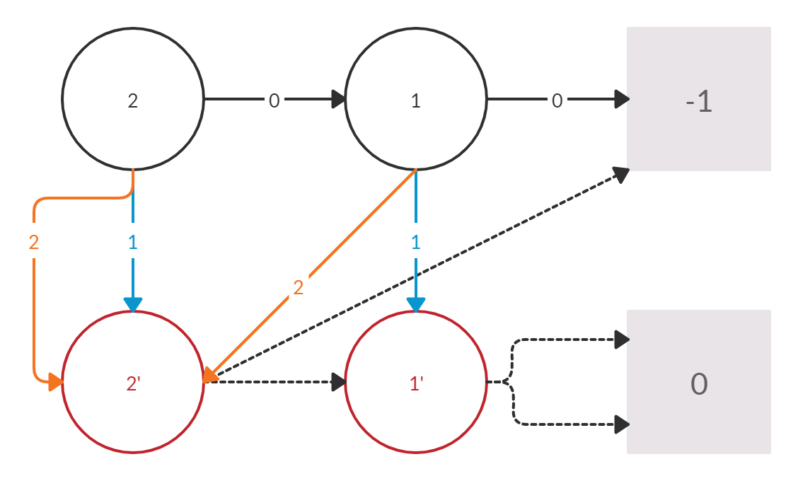
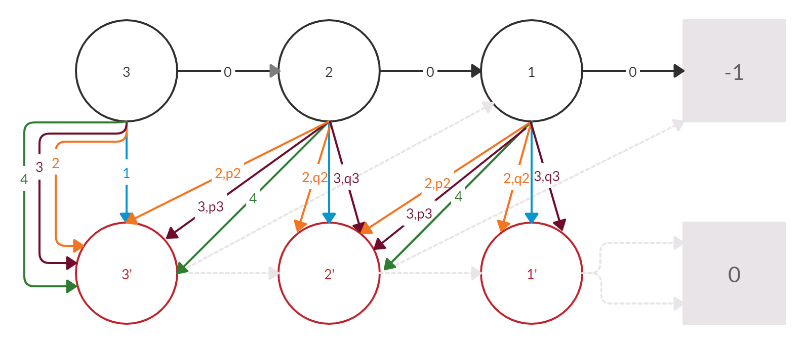
Figures 1, 2 and 3 show the MDP graph for (n=2,k=3)formulae-sequence𝑛2𝑘3(n=2,k=3), (n=3,k=3)formulae-sequence𝑛3𝑘3(n=3,k=3) and (n=3,k=5)formulae-sequence𝑛3𝑘5(n=3,k=5) respectively.

Refer to caption
Figure 1: (2,3)23\mathcal{F}(2,3), Sinks are square vertices (Best viewed in color)
Refer to caption
Figure 2: (3,3)33\mathcal{F}(3,3) (Best viewed in color)
Refer to caption
Figure 3: (3,5)35\mathcal{F}(3,5) (Best viewed in color)

V Simple Policy Iteration

In Simple Policy Iteration (SPI), the policy of an arbitrary improvable state is switched to an arbitrary improving action. Specifically, the improvable state with the highest index is selected and its policy is switched to the improvable action with the highest index.

We denote the number of iterations taken by SPI for the a n𝑛n-state, k𝑘k-action MDP from the above family with an initial policy of SnSn1S2S1=0000subscript𝑆𝑛subscript𝑆𝑛1subscript𝑆2subscript𝑆10000S_{n}S_{n-1}\ldots S_{2}S_{1}=00\ldots 00 to converge to the optimum policy as 𝒩(n,k)𝒩𝑛𝑘\mathcal{N}(n,k). We shall experimentally show and later prove that:

𝒩(n,k)=(3+k)2n22𝒩𝑛𝑘3𝑘superscript2𝑛22\mathcal{N}(n,k)=(3+k)2^{n-2}-2 (1)

VI Experiments

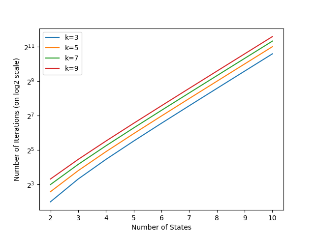
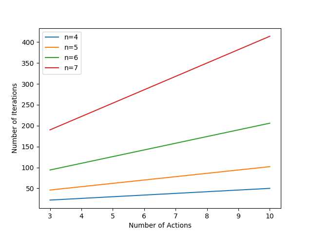
Figure 4 shows a plot of the number of iterations against the number of states and actions. Table II in the appendix contains number of iterations for for all n,k𝑛𝑘n,k pairs upto n=k=10𝑛𝑘10n=k=10.

Refer to caption
Refer to caption
Figure 4: (Top) Variation of number of iterations with number of states for fixed number of actions. The vertical scale is in logarithm with base 2. The line is almost linear which justifies the exponential dependence with number of states. (Bottom) Variation of number of iterations with number of action for fixed k. This dependence is linear with an increasing slope.

We next describe how the switching happens for the MDP graph (n=2,k=3)formulae-sequence𝑛2𝑘3(n=2,k=3) shown in Figure 1. Initially both vertices 1 and 2 are switchable because:

Q(2,1)=Q(2,2)=12>Q(2,0)=1𝑄21𝑄2212𝑄201\displaystyle Q(2,1)=Q(2,2)=-\frac{1}{2}>Q(2,0)=-1
Q(1,1)=0>Q(1,2)=12>Q(1,0)=1𝑄110𝑄1212𝑄101\displaystyle Q(1,1)=0>Q(1,2)=-\frac{1}{2}>Q(1,0)=-1

According to the switching rule, state 2 switches to action 1. At this point only state 1 is improvable. So state 1 switches to the highest indexed improvable action which is 2. After this switch state 1 is again the only improvable state and it switches to action 1. This switch causes state 1 to attain its best possible value (0) and also makes state 2 improvable because:

Q(2,0)>Q(2,2)=Q(2,1)12𝑄20𝑄22𝑄2112Q(2,0)>Q(2,2)=Q(2,1)-\frac{1}{2}

Hence state 2 switches to action 0 and SPI converges to the optimal policy. The switching has been shown in the table below.

TABLE I: Switching sequence for n=2,k=3formulae-sequence𝑛2𝑘3n=2,k=3
t π(2)π(1)𝜋2𝜋1\pi(2)\quad\pi(1) Vt(2)superscript𝑉𝑡2V^{t}(2) Vt(1)superscript𝑉𝑡1V^{t}(1)
0 00000\quad 0 11-1 11-1
1 20202\quad 0 1212-\frac{1}{2} 11-1
2 22222\quad 2 1212-\frac{1}{2} 1212-\frac{1}{2}
3 21212\quad 1 1212-\frac{1}{2} 00
4 01010\quad 1 00 00

VII Proof

The proof of the recursive relation requires the construction of a complementary family of MDPs, Csubscript𝐶\mathcal{F}_{C}, which have the same structure and transition probabilities as \mathcal{F} but sink values of the opposite relative order. We shall denote the n𝑛n states, k𝑘k actions MDP belonging to this complementary family as C(n,k)subscript𝐶𝑛𝑘\mathcal{F}_{C}(n,k) henceforth. By Corollary 7.2, the complementary MDP is set to have sink rewards of (1,0). Note that the optimal policy for C(n,k)subscript𝐶𝑛𝑘\mathcal{F}_{C}(n,k) is SnSn1S2S1=0000subscript𝑆𝑛subscript𝑆𝑛1subscript𝑆2subscript𝑆10000S_{n}S_{n-1}\ldots S_{2}S_{1}=00\ldots 00. We denote the number of iterations taken by SPI for a n𝑛n-state, k𝑘k-action complementary MDP beginning with a policy of SnSn1S2S1=0001subscript𝑆𝑛subscript𝑆𝑛1subscript𝑆2subscript𝑆10001S_{n}S_{n-1}\ldots S_{2}S_{1}=00\ldots 01 as 𝒩C(n,k)subscript𝒩𝐶𝑛𝑘\mathcal{N}_{C}(n,k).

Lemma 7.1.

Policy iteration for the n-state, k-action MDP from family \mathcal{F} and Csubscript𝐶\mathcal{F}_{C} is invariant to the actual value of sink values, and only depends on their relative values

Proof.

Let sink values be (α,β)𝛼𝛽(\alpha,\beta) = (k1subscript𝑘1k_{1},k2subscript𝑘2k_{2}).
The transformation of the sink reward maintaining the relative order can be expressed as by a linear transform:

𝒯:(k1,k2)(A×k1+B,A×k2+B):𝒯subscript𝑘1subscript𝑘2𝐴subscript𝑘1𝐵𝐴subscript𝑘2𝐵\mathcal{T}:(k_{1},k_{2})\rightarrow(A\times k_{1}+B,A\times k_{2}+B)

where A+,Bformulae-sequence𝐴superscript𝐵A\in\mathbb{R}^{+},B\in\mathbb{R}.
The linear transformation of the sink rewards would result in the same transformation to the Q𝑄Q and V𝑉V values. As A>0𝐴0A>0, the relative orders in Q-values do no change and so the switches do not change.

Corollary 7.2.

Sink values for the MDPs from family \mathcal{F} can be set to (α,β)𝛼𝛽(\alpha,\beta) = (-1,0) and those for the complementary MDPs can be set to (α,β)𝛼𝛽(\alpha,\beta) =(1,0) without loss of generality.

Lemma 7.3.

At any time t, for (n,k)𝑛𝑘\mathcal{F}(n,k),

Qt(1,1)>Qt(1,2)>Qt(1,3)>>Qt(1,k1)>Qt(1,0)superscript𝑄𝑡11superscript𝑄𝑡12superscript𝑄𝑡13superscript𝑄𝑡1𝑘1superscript𝑄𝑡10Q^{t}(1,1)>Q^{t}(1,2)>Q^{t}(1,3)>\ldots>Q^{t}(1,k-1)>Q^{t}(1,0)
Proof.

By the structure of the MDP, Vt(2)=12superscript𝑉𝑡superscript212V^{t}(2^{\prime})=-\frac{1}{2} and Vt(1)=0superscript𝑉𝑡superscript10V^{t}(1^{\prime})=0
This results in

Qt(1,i)={1, if i=00, if i=11/2, if i=k1superscript𝑄𝑡1𝑖cases1 if 𝑖00 if 𝑖112 if 𝑖𝑘1Q^{t}(1,i)=\begin{cases}-1,&\text{ if }i=0\\ 0,&\text{ if }i=1\\ -1/2,&\text{ if }i=k-1\\ \end{cases}

By the construction of \mathcal{F},

pisubscript𝑝𝑖\displaystyle p_{i} (0,1)i{2,3,..k1}\displaystyle\in(0,1)\quad\forall i\in\{2,3,..k-1\}
pjsubscript𝑝𝑗\displaystyle p_{j} >pij>i,i,j{2,3,..k1}\displaystyle>p_{i}\quad\forall j>i,i,j\in\{2,3,..k-1\}

Plugging the values of Qt(1,)superscript𝑄𝑡1Q^{t}(1,\cdot) will yield the desired relation. ∎

Lemma 7.4.

At any time t, for C(n,k)subscript𝐶𝑛𝑘\mathcal{F}_{C}(n,k),

Qt(1,0)>Qt(1,k1)>Qt(1,k2)>>Qt(1,2)>Qt(1,1)superscript𝑄𝑡10superscript𝑄𝑡1𝑘1superscript𝑄𝑡1𝑘2superscript𝑄𝑡12superscript𝑄𝑡11Q^{t}(1,0)>Q^{t}(1,k-1)>Q^{t}(1,k-2)>\ldots>Q^{t}(1,2)>Q^{t}(1,1)
Proof.

By the structure of the MDP, Vt(2)=12superscript𝑉𝑡superscript212V^{t}(2^{\prime})=\frac{1}{2} and Vt(1)=0superscript𝑉𝑡superscript10V^{t}(1^{\prime})=0
This results in

Qt(1,i)={1, if i=00, if i=1pi/2,i>1superscript𝑄𝑡1𝑖cases1 if 𝑖00 if 𝑖1subscript𝑝𝑖2for-all𝑖1Q^{t}(1,i)=\begin{cases}1,&\text{ if }i=0\\ 0,&\text{ if }i=1\\ p_{i}/2,&\forall i>1\end{cases}

By the construction of Csubscript𝐶\mathcal{F}_{C},

pisubscript𝑝𝑖\displaystyle p_{i} (0,1)i{2,3,..k1}\displaystyle\in(0,1)\quad\forall i\in\{2,3,..k-1\}
pjsubscript𝑝𝑗\displaystyle p_{j} >pij>i,i,j{2,3,..k1}\displaystyle>p_{i}\quad\forall j>i,i,j\in\{2,3,..k-1\}

Plugging the values of Qt(1,)superscript𝑄𝑡1Q^{t}(1,\cdot) will yield the desired relation. ∎

Lemma 7.5 (Baseline).
𝒩(2,k)=k+1k3formulae-sequence𝒩2𝑘𝑘1for-all𝑘3\mathcal{N}(2,k)=k+1\quad\forall k\geq 3
Proof.

We have the initial policy π0=S2S1=00superscript𝜋0subscript𝑆2subscript𝑆100\pi^{0}=S_{2}S_{1}=00 and

Q0(2,0)=1 and Q0(2,a)=12a>0formulae-sequencesuperscript𝑄0201 and superscript𝑄02𝑎12for-all𝑎0Q^{0}(2,0)=-1\text{ and }Q^{0}(2,a)=-\frac{1}{2}\quad\forall a>0

As per our definition of SPI, policy with highest improvable action will be chosen. Consequently,

π1=S2S1=k1,0formulae-sequencesuperscript𝜋1subscript𝑆2subscript𝑆1𝑘10\pi^{1}=S_{2}S_{1}=k-1,0

Next we have Q1(2,k1)Q(2,a)asuperscript𝑄12𝑘1𝑄2𝑎for-all𝑎Q^{1}(2,k-1)\geq Q(2,a)\quad\forall a, we focus on improving state 1. We observe

Q1(1,0)=1 and Q1(1,k1)=12superscript𝑄1101 and superscript𝑄11𝑘112Q^{1}(1,0)=-1\text{ and }Q^{1}(1,k-1)=-\frac{1}{2}

Hence,

π2=S2S1=k1,k1formulae-sequencesuperscript𝜋2subscript𝑆2subscript𝑆1𝑘1𝑘1\pi^{2}=S_{2}S_{1}=k-1,k-1

Even now, state 2 is not improvable and we have

Q2(1,k2)=pk2212superscript𝑄21𝑘2subscript𝑝𝑘2212Q^{2}(1,k-2)=\frac{-p_{k-2}}{2}\geq\frac{-1}{2}

by our choice of pk2subscript𝑝𝑘2p_{k-2}. Hence,

π3=S2S1=k1,k2formulae-sequencesuperscript𝜋3subscript𝑆2subscript𝑆1𝑘1𝑘2\pi^{3}=S_{2}S_{1}=k-1,k-2

Now,

Q3(2,0)=V3(1)=pk22>12=Q3(2,a)a0formulae-sequencesuperscript𝑄320superscript𝑉31subscript𝑝𝑘2212superscript𝑄32𝑎for-all𝑎0Q^{3}(2,0)=V^{3}(1)=\frac{-p_{k-2}}{2}>\frac{-1}{2}=Q^{3}(2,a)\quad\forall a\neq 0

So,

π4=S2S1=0(k2)superscript𝜋4subscript𝑆2subscript𝑆10𝑘2\pi^{4}=S_{2}S_{1}=0(k-2)

For all consequent ithsuperscript𝑖𝑡i^{th} iteration,

Qi(2,0)=Vi(1)>12 but Qi(2,a)=Vi(2)=12superscript𝑄𝑖20superscript𝑉𝑖112 but superscript𝑄𝑖2𝑎superscript𝑉𝑖superscript212Q^{i}(2,0)=V^{i}(1)>\frac{-1}{2}\text{ but }Q^{i}(2,a)=V^{i}(2^{\prime})=\frac{-1}{2}

and hence only S1subscript𝑆1S_{1} is improvable. From Lemma 7.4, we have

Q4(1,1)>Q4(1,2)>Q4(1,k2)superscript𝑄411superscript𝑄412superscript𝑄41𝑘2Q^{4}(1,1)>Q^{4}(1,2)>\ldots Q^{4}(1,k-2)

Thus, the next k3𝑘3k-3 iterations are required to reach

πk+1=S2S1=01superscript𝜋𝑘1subscript𝑆2subscript𝑆101\pi^{k+1}=S_{2}S_{1}=01

thus giving a total of k+1𝑘1k+1 iterations.

Lemma 7.6.

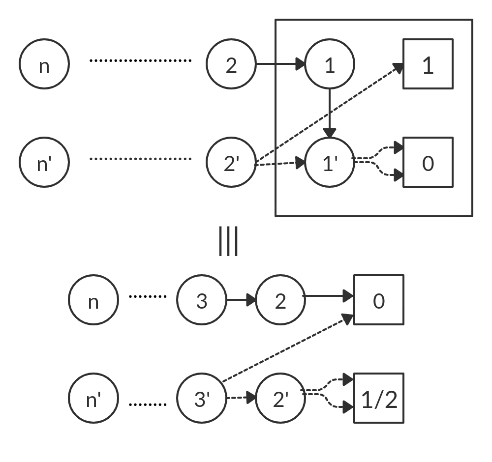
For the C(n,k)subscript𝐶𝑛𝑘\mathcal{F}_{C}(n,k) with initial policy: SnSn1S2S1=0001subscript𝑆𝑛subscript𝑆𝑛1subscript𝑆2subscript𝑆10001S_{n}S_{n-1}\ldots S_{2}S_{1}=00\ldots 01 it takes exactly 𝒩(n1,k)𝒩𝑛1𝑘\mathcal{N}(n-1,k) iterations before policy at the first state vertex changes.

Proof.
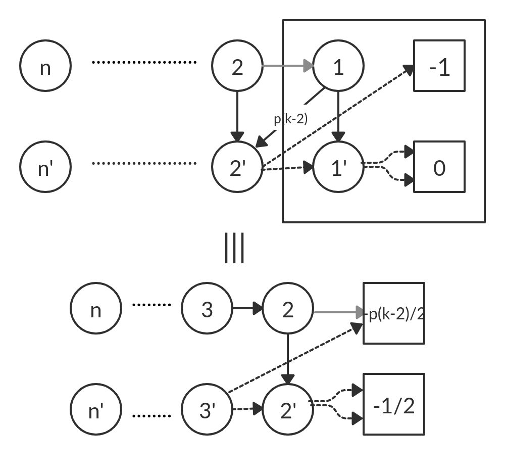
Due to the switching rule of SPI, S1subscript𝑆1S_{1} will only change when all the other state vertices are not improvable. Until all the higher states finish improving, the current sinks and state 1 can be effectively reduced to new sinks with (α,β)=(0,12)𝛼𝛽012(\alpha,\beta)=(0,\frac{1}{2}). This reduction is shown in Figure 5. Using Lemma 7.1 the resultant MDP is equivalent to (n1,k)𝑛1𝑘\mathcal{F}(n-1,k) having initial policy SnSn1S2=0000subscript𝑆𝑛subscript𝑆𝑛1subscript𝑆20000S_{n}S_{n-1}\ldots S_{2}=00\ldots 00. This MDP takes N(n1,k)𝑁𝑛1𝑘N(n-1,k) iterations to converge to the optimal policy SnSn1S2=0001subscript𝑆𝑛subscript𝑆𝑛1subscript𝑆20001S_{n}S_{n-1}\ldots S_{2}=00\ldots 01. By this logic after the 𝒩(n1,k)𝒩𝑛1𝑘\mathcal{N}(n-1,k) iterations, the policy would be SnSn1S2S1=0011subscript𝑆𝑛subscript𝑆𝑛1subscript𝑆2subscript𝑆10011S_{n}S_{n-1}\ldots S_{2}S_{1}=00\ldots 11

Refer to caption
Figure 5: Reducing C(n,k)subscript𝐶𝑛𝑘\mathcal{F}_{C}(n,k) to (n1,k)𝑛1𝑘\mathcal{F}(n-1,k) with respect to its initial policy
Lemma 7.7.

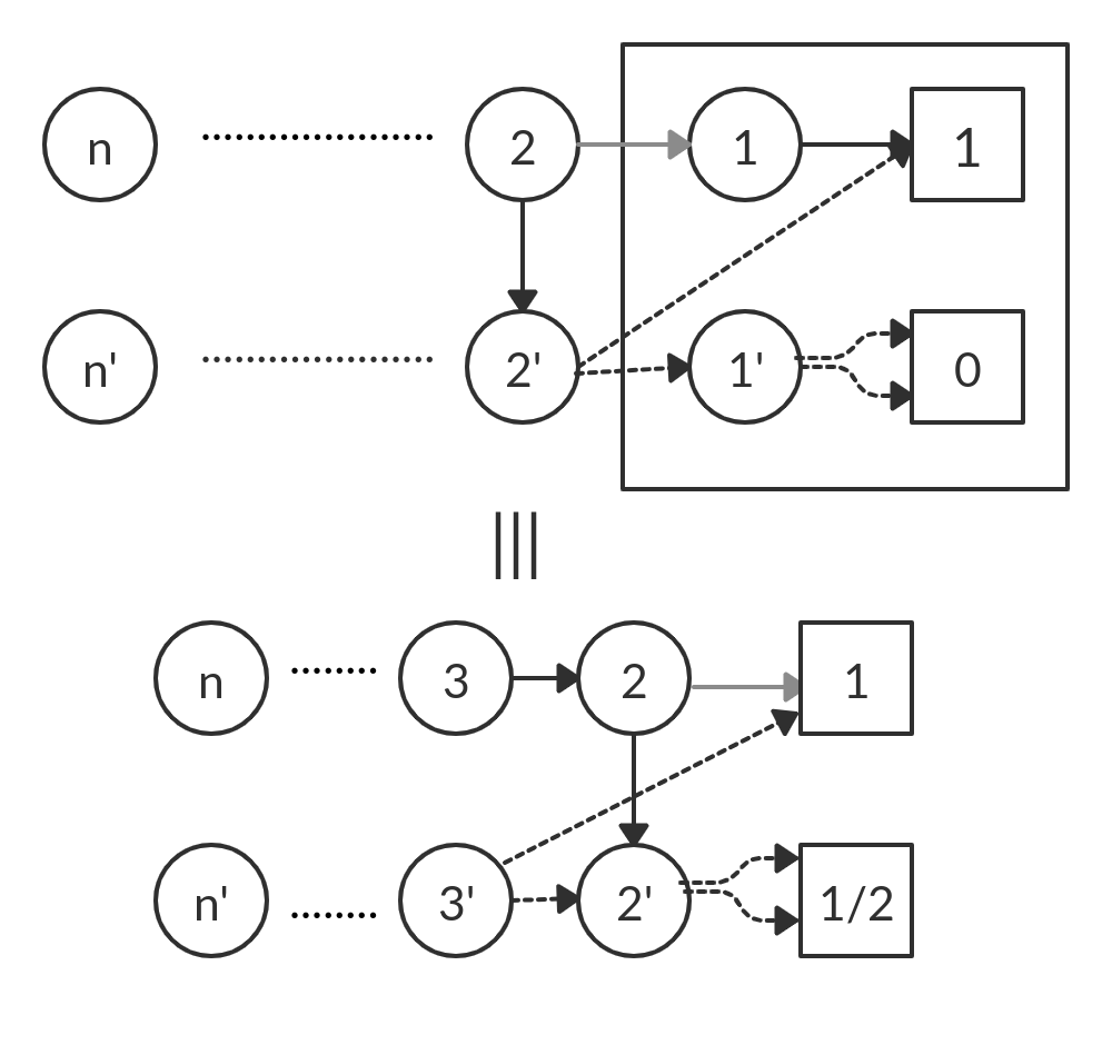
If πt=SnSn1S2S1=0011superscript𝜋𝑡subscript𝑆𝑛subscript𝑆𝑛1subscript𝑆2subscript𝑆10011\pi^{t}=S_{n}S_{n-1}\ldots S_{2}S_{1}=00\ldots 11 for C(n,k)subscript𝐶𝑛𝑘\mathcal{F}_{C}(n,k), the next 2 switches of simple policy iteration occur at state 1

Proof.

Using Lemma 7.6 the policy πtsuperscript𝜋𝑡\pi^{t} is optimal with respect to the states n,n13,2𝑛𝑛132n,n-1\ldots 3,2 and is SnSn1S2=0001subscript𝑆𝑛subscript𝑆𝑛1subscript𝑆20001S_{n}S_{n-1}\ldots S_{2}=00\ldots 01. Vertex 1 is the only improvable state and according to Lemma 7.4 it switches to its highest indexed improvable action k1𝑘1k-1. Hence the policy becomes SnSn1S2S1=0,01,k1subscript𝑆𝑛subscript𝑆𝑛1subscript𝑆2subscript𝑆1001𝑘1S_{n}S_{n-1}\ldots S_{2}S_{1}=0,0\ldots 1,k-1. With respect to the current policy the sinks and state 1 can be effectively reduced to new sinks with (α,β)=(12,12)𝛼𝛽1212(\alpha,\beta)=(\frac{1}{2},\frac{1}{2}). This reduction is shown in Figure 6. The action values are equal for equal sink values and hence the policy for states n,n13,2𝑛𝑛132n,n-1\ldots 3,2 is still optimal. State 1 is still the only improvable state and according to Lemma 7.4 it switches to the next improvable action 0. This completes the proof. The policy would now be SnSn1S2S1=0010subscript𝑆𝑛subscript𝑆𝑛1subscript𝑆2subscript𝑆10010S_{n}S_{n-1}\ldots S_{2}S_{1}=00\ldots 10

Refer to caption
Figure 6: Reducing C(n,k)subscript𝐶𝑛𝑘\mathcal{F}_{C}(n,k) with respect to the policy SnSn1S2S1=0,01,k1subscript𝑆𝑛subscript𝑆𝑛1subscript𝑆2subscript𝑆1001𝑘1S_{n}S_{n-1}\ldots S_{2}S_{1}=0,0\ldots 1,k-1
Lemma 7.8.

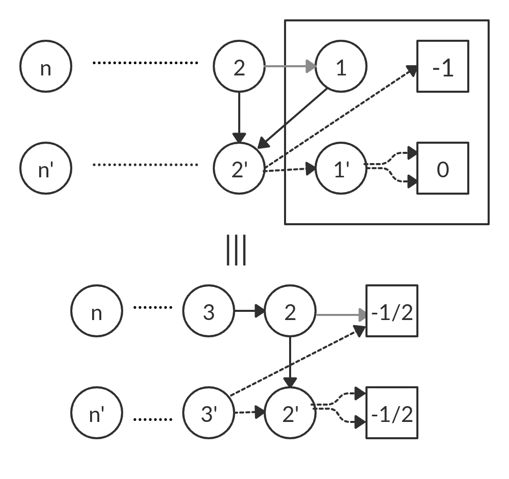
If πt=SnSn1S2S1=0010superscript𝜋𝑡subscript𝑆𝑛subscript𝑆𝑛1subscript𝑆2subscript𝑆10010\pi^{t}=S_{n}S_{n-1}\ldots S_{2}S_{1}=00\ldots 10 for C(n,k)subscript𝐶𝑛𝑘\mathcal{F}_{C}(n,k), it takes 𝒩C(n1,k)subscript𝒩𝐶𝑛1𝑘\mathcal{N}_{C}(n-1,k) iterations to converge to optimal policy.

Proof.

With respect to πt=SnSn1S2S1=0010superscript𝜋𝑡subscript𝑆𝑛subscript𝑆𝑛1subscript𝑆2subscript𝑆10010\pi^{t}=S_{n}S_{n-1}\ldots S_{2}S_{1}=00\ldots 10 the sinks and state 1 can be effectively reduced to new sinks with (α,β)=(1,12)𝛼𝛽112(\alpha,\beta)=(1,\frac{1}{2}). This reduction is shown in Figure 7. Invoking Lemma 7.1 this MDP is equivalent to C(n1,k)subscript𝐶𝑛1𝑘\mathcal{F}_{C}(n-1,k) with initial policy SnSn1S2=0001subscript𝑆𝑛subscript𝑆𝑛1subscript𝑆20001S_{n}S_{n-1}\ldots S_{2}=00\ldots 01 and hence takes 𝒩C(n1,k)subscript𝒩𝐶𝑛1𝑘\mathcal{N}_{C}(n-1,k) iterations to converge to optimal policy Sn1S2=0000subscript𝑆𝑛1subscript𝑆20000S_{n-1}\ldots S_{2}=00\ldots 00. The complete policy is now Sn1S2S1=0000subscript𝑆𝑛1subscript𝑆2subscript𝑆10000S_{n-1}\ldots S_{2}S_{1}=00\ldots 00 which is also the optimal policy for FC(n,k)subscript𝐹𝐶𝑛𝑘F_{C}(n,k)

Refer to caption
Figure 7: Reducing C(n,k)subscript𝐶𝑛𝑘\mathcal{F}_{C}(n,k) to C(n1,k)subscript𝐶𝑛1𝑘\mathcal{F}_{C}(n-1,k)with respect to policy SnSn1S2S1=0,01,0subscript𝑆𝑛subscript𝑆𝑛1subscript𝑆2subscript𝑆10010S_{n}S_{n-1}\ldots S_{2}S_{1}=0,0\ldots 1,0
Theorem 7.9.
𝒩C(n+1,k)=𝒩(n,k)+2+𝒩C(n,k)subscript𝒩𝐶𝑛1𝑘𝒩𝑛𝑘2subscript𝒩𝐶𝑛𝑘\mathcal{N}_{C}(n+1,k)=\mathcal{N}(n,k)+2+\mathcal{N}_{C}(n,k) (2)
Proof.

This can be proved by sequentially applying Lemmas 7.6-7.8 ∎

Lemma 7.10.

For t (n,k)𝑛𝑘\mathcal{F}(n,k) having initial policy SnSn1S2S1=0000subscript𝑆𝑛subscript𝑆𝑛1subscript𝑆2subscript𝑆10000S_{n}S_{n-1}\ldots S_{2}S_{1}=00\ldots 00, it takes exactly 𝒩(n1,k)𝒩𝑛1𝑘\mathcal{N}(n-1,k) iterations before policy at the first state vertex changes.

Proof.

Due to the switching rule of SPI, S1subscript𝑆1S_{1} will only change when all the other state vertices are not improvable. Until the higher states improve, the current sinks and state 1 can be effectively reduced to new sinks with (α,β)=(1,12)𝛼𝛽112(\alpha,\beta)=(-1,-\frac{1}{2}). This reduction is shown in Figure 8. Using Lemma 7.1 the resultant MDP is equivalent to (n1,k)𝑛1𝑘\mathcal{F}(n-1,k) having initial policy SnSn1S2=0000subscript𝑆𝑛subscript𝑆𝑛1subscript𝑆20000S_{n}S_{n-1}\ldots S_{2}=00\ldots 00. This MDP takes N(n1,k)𝑁𝑛1𝑘N(n-1,k) iterations to converge to the optimal policy SnSn1S2=0001subscript𝑆𝑛subscript𝑆𝑛1subscript𝑆20001S_{n}S_{n-1}\ldots S_{2}=00\ldots 01. By this logic after the 𝒩(n1,k)𝒩𝑛1𝑘\mathcal{N}(n-1,k) iterations, the policy would be SnSn1S2S1=0010subscript𝑆𝑛subscript𝑆𝑛1subscript𝑆2subscript𝑆10010S_{n}S_{n-1}\ldots S_{2}S_{1}=00\ldots 10

Refer to caption
Figure 8: Reducing (n,k)𝑛𝑘\mathcal{F}(n,k) to (n1,k)𝑛1𝑘\mathcal{F}(n-1,k) with respect to its initial policy
Lemma 7.11.

If πt=SnSn1S2S1=0010superscript𝜋𝑡subscript𝑆𝑛subscript𝑆𝑛1subscript𝑆2subscript𝑆10010\pi^{t}=S_{n}S_{n-1}\ldots S_{2}S_{1}=00\ldots 10, the next 2 switches of simple policy iteration occur at vertex 1

Proof.

Using Lemma 7.3 the policy πtsuperscript𝜋𝑡\pi^{t} is optimal with respect to the states n,n13,2𝑛𝑛132n,n-1\ldots 3,2 and is SnSn1S2=0001subscript𝑆𝑛subscript𝑆𝑛1subscript𝑆20001S_{n}S_{n-1}\ldots S_{2}=00\ldots 01. Vertex 1 is the only improvable state and according to Lemma 7.3 it switches to its highest indexed improvable action k1𝑘1k-1. Hence the policy becomes SnSn1S2S1=0,01,k1subscript𝑆𝑛subscript𝑆𝑛1subscript𝑆2subscript𝑆1001𝑘1S_{n}S_{n-1}\ldots S_{2}S_{1}=0,0\ldots 1,k-1. With respect to the current policy the sinks and state 1 can be effectively reduced to new sinks with (α,β)=(12,12)𝛼𝛽1212(\alpha,\beta)=(-\frac{1}{2},-\frac{1}{2}). This reduction is shown in Figure 9. The action values are equal for equal sink values and hence the policy for states n,n13,2𝑛𝑛132n,n-1\ldots 3,2 is still optimal. State 1 is still the only improvable state and according to Lemma 7.3 it switches to the next improvable action k-2. This completes the proof. The policy would now be SnSn1S2S1=001,k2subscript𝑆𝑛subscript𝑆𝑛1subscript𝑆2subscript𝑆1001𝑘2S_{n}S_{n-1}\ldots S_{2}S_{1}=00\ldots 1,k-2

Refer to caption
Figure 9: Reducing (n,k)𝑛𝑘\mathcal{F}(n,k) with respect to policy SnSn1S2S1=0,01,k1subscript𝑆𝑛subscript𝑆𝑛1subscript𝑆2subscript𝑆1001𝑘1S_{n}S_{n-1}\ldots S_{2}S_{1}=0,0\ldots 1,k-1
Lemma 7.12.

If πt=SnSn1S2S1=001,k2formulae-sequencesuperscript𝜋𝑡subscript𝑆𝑛subscript𝑆𝑛1subscript𝑆2subscript𝑆1001𝑘2\pi^{t}=S_{n}S_{n-1}\ldots S_{2}S_{1}=00\ldots 1,k-2 for (n,k)𝑛𝑘\mathcal{F}(n,k), it takes 𝒩C(n1,k)subscript𝒩𝐶𝑛1𝑘\mathcal{N}_{C}(n-1,k) iterations before policy at the first state vertex changes.

Proof.

With respect to πt=SnSn1S2S1=001,k2formulae-sequencesuperscript𝜋𝑡subscript𝑆𝑛subscript𝑆𝑛1subscript𝑆2subscript𝑆1001𝑘2\pi^{t}=S_{n}S_{n-1}\ldots S_{2}S_{1}=00\ldots 1,k-2 the sinks and state 1 can be effectively reduced to new sinks with (α,β)=(pk22,12)𝛼𝛽subscript𝑝𝑘2212(\alpha,\beta)=(-\frac{p_{k-2}}{2},-\frac{1}{2}). This reduction is shown in Figure 10. Invoking Lemma 7.1 this MDP is equivalent to C(n1,k)subscript𝐶𝑛1𝑘\mathcal{F}_{C}(n-1,k) with initial policy SnSn1S2=0001subscript𝑆𝑛subscript𝑆𝑛1subscript𝑆20001S_{n}S_{n-1}\ldots S_{2}=00\ldots 01 and hence takes 𝒩C(n1,k)subscript𝒩𝐶𝑛1𝑘\mathcal{N}_{C}(n-1,k) iterations to converge to optimal policy Sn1S2=0000subscript𝑆𝑛1subscript𝑆20000S_{n-1}\ldots S_{2}=00\ldots 00. The complete policy is now Sn1S2S1=000,k2subscript𝑆𝑛1subscript𝑆2subscript𝑆1000𝑘2S_{n-1}\ldots S_{2}S_{1}=00\ldots 0,k-2

Refer to caption
Figure 10: Reducing (n,k)𝑛𝑘\mathcal{F}(n,k) to c(n1,k)subscript𝑐𝑛1𝑘\mathcal{F}_{c}(n-1,k) with respect to policy SnSn1S2S1=0,01,k2subscript𝑆𝑛subscript𝑆𝑛1subscript𝑆2subscript𝑆1001𝑘2S_{n}S_{n-1}\ldots S_{2}S_{1}=0,0\ldots 1,k-2
Lemma 7.13.

If πt=SnSn1S2S1=0,0,,k2formulae-sequencesuperscript𝜋𝑡subscript𝑆𝑛subscript𝑆𝑛1subscript𝑆2subscript𝑆100𝑘2\pi^{t}=S_{n}S_{n-1}\ldots S_{2}S_{1}=0,0,\ldots,k-2 for (n,k)𝑛𝑘\mathcal{F}(n,k), it takes k3𝑘3k-3 iterations to converge to optimal policy.

Proof.

With respect to πt=SnSn1S2S1=0,0,,k2formulae-sequencesuperscript𝜋𝑡subscript𝑆𝑛subscript𝑆𝑛1subscript𝑆2subscript𝑆100𝑘2\pi^{t}=S_{n}S_{n-1}\ldots S_{2}S_{1}=0,0,\ldots,k-2 for (n,k)𝑛𝑘\mathcal{F}(n,k) the sinks and state 1 can be effectively reduced to new sinks with (α,β)=(pk22,12)𝛼𝛽subscript𝑝𝑘2212(\alpha,\beta)=(-\frac{p_{k-2}}{2},-\frac{1}{2}). Invoking Lemma 7.1 this MDP is equivalent to C(n1,k)subscript𝐶𝑛1𝑘\mathcal{F}_{C}(n-1,k) with initial policy SnSn1S2=0000subscript𝑆𝑛subscript𝑆𝑛1subscript𝑆20000S_{n}S_{n-1}\ldots S_{2}=00\ldots 00 and hence this is already optimal. This means that only change that will happen is at state 1. Using Lemma 7.3 we get an incremental change in the improvable policy. Also, at any subsequent stage i𝑖i the value of sink is (α,β)=(pi2,12)𝛼𝛽subscript𝑝𝑖212(\alpha,\beta)=(-\frac{p_{i}}{2},-\frac{1}{2}), which again implies only state 1 can be improved. Hence it would take k3𝑘3k-3 iterations to converge to the optimal policy SnSn1S2S1=0001subscript𝑆𝑛subscript𝑆𝑛1subscript𝑆2subscript𝑆10001S_{n}S_{n-1}\ldots S_{2}S_{1}=00\ldots 01

Theorem 7.14.
𝒩(n+1,k)=𝒩(n,k)+2+𝒩C(n,k)+(k3)𝒩𝑛1𝑘𝒩𝑛𝑘2subscript𝒩𝐶𝑛𝑘𝑘3\mathcal{N}(n+1,k)=\mathcal{N}(n,k)+2+\mathcal{N}_{C}(n,k)+(k-3) (3)
Proof.

This can be be proven by sequentially applying Lemmas 7.10-7.13. ∎

Theorem 7.15 (Recursive Relation).
𝒩(n+1,k)=2×𝒩(n,k)+2𝒩𝑛1𝑘2𝒩𝑛𝑘2\mathcal{N}(n+1,k)=2\times\mathcal{N}(n,k)+2
Proof.

Subtracting eq.(2) from eq.(3), we get the relation:

𝒩(n+1,k)𝒩C(n+1,k)=(k3)𝒩𝑛1𝑘subscript𝒩𝐶𝑛1𝑘𝑘3\mathcal{N}(n+1,k)-\mathcal{N}_{C}(n+1,k)=(k-3)

As the RHS of the above is independent of n𝑛n, we can replace n+1𝑛1n+1 with n𝑛n to get

𝒩C(n,k)=𝒩(n,k)(k3)subscript𝒩𝐶𝑛𝑘𝒩𝑛𝑘𝑘3\mathcal{N}_{C}(n,k)=\mathcal{N}(n,k)-(k-3)

Substituting 𝒩C(n,k)subscript𝒩𝐶𝑛𝑘\mathcal{N}_{C}(n,k) from the above equation into eq.(3) completes the proof. ∎

Theorem 7.16.
𝒩(n,k)=(3+k)2n22𝒩𝑛𝑘3𝑘superscript2𝑛22\mathcal{N}(n,k)=(3+k)2^{n-2}-2
Proof.

For a fixed k, use the baseline from lemma 7.5 and apply the recursive relation described by theorem 7.15 to complete the proof.

𝒩(2,k)𝒩2𝑘\displaystyle\mathcal{N}(2,k) =k+1absent𝑘1\displaystyle=k+1
𝒩(3,k)𝒩3𝑘\displaystyle\mathcal{N}(3,k) =2(k+1)+2absent2𝑘12\displaystyle=2(k+1)+2
𝒩(4,k)𝒩4𝑘\displaystyle\mathcal{N}(4,k) =22(k+1)+22+2absentsuperscript22𝑘1superscript222\displaystyle=2^{2}(k+1)+2^{2}+2
\displaystyle\;\;\vdots
𝒩(n,k)𝒩𝑛𝑘\displaystyle\mathcal{N}(n,k) =2n2(k+1)+i=1n22iabsentsuperscript2𝑛2𝑘1superscriptsubscript𝑖1𝑛2superscript2𝑖\displaystyle=2^{n-2}(k+1)+\sum_{i=1}^{n-2}2^{i}
=(3+k)2n22absent3𝑘superscript2𝑛22\displaystyle=(3+k)2^{n-2}-2
=(3+k)2N/232absent3𝑘superscript2𝑁232\displaystyle=(3+k)2^{N/2-3}-2

VIII Conclusion

In this work, we established a generalized lower bound on the number of iterations for a N𝑁N state, k𝑘k action MDP. We demonstrated the MDP formulation and proved a lower bound of 𝒪((3+k)2N/23)𝒪3𝑘superscript2𝑁23\mathcal{O}\big{(}(3+k)2^{N/2-3}\big{)}. However, we do not reject the existence of an MDP with a tighter lower bound, say, 𝒪(kN)𝒪superscript𝑘𝑁\mathcal{O}\big{(}k^{N}\big{)}. Out of all of family of MDP that we constructed and verified, most of them were 𝒪(2N+k)𝒪superscript2𝑁𝑘\mathcal{O}\big{(}2^{N}+k\big{)} and a few were 𝒪(k.2N)𝒪𝑘superscript.2𝑁\mathcal{O}\big{(}k.{2}^{N}\big{)}. Considering the switching rule employed by our construction, and the family of other MDPs we tested, finding an MDP with a tighter lower bound would be an interesting extension to our work.

IX Additional Result

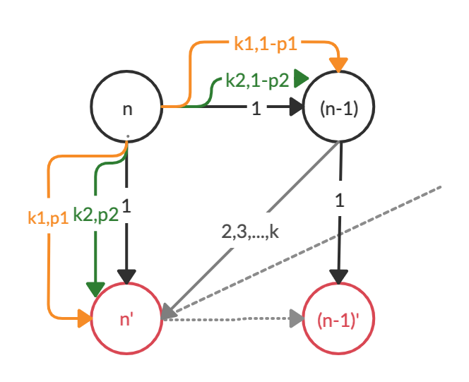
We observed that the pattern used to define multiple actions was not being followed in very last states, which had scope of improvement. A simple modification to the actions from the final state improve the baseline from

𝒩(2,k)=k+1k3formulae-sequence𝒩2𝑘𝑘1for-all𝑘3\mathcal{N}(2,k)=k+1\quad\forall k\geq 3

to

𝒩(2,k)=2kk3formulae-sequence𝒩2𝑘2𝑘for-all𝑘3\mathcal{N}(2,k)=2k\quad\forall k\geq 3

which futher increases the lower bound from 𝒪((3+k)2N/23)𝒪3𝑘superscript2𝑁23\mathcal{O}\big{(}(3+k)2^{N/2-3}\big{)} to 𝒪((1+k)2N/22)𝒪1𝑘superscript2𝑁22\mathcal{O}\big{(}(1+k)2^{N/2-2}\big{)} which was confirmed experimentally. Since the change is only at the final state, we believe that the rest of the proof will remain the same. The variation in the MDP has been shown in the Appendix Fig.11. k1,k2𝑘1𝑘2k1,k2 are actions with probability p1,p2𝑝1𝑝2p1,p2 respectively and k1>k2p1>p2𝑘1𝑘2𝑝1𝑝2k1>k2\implies p1>p2.

References

  • [1] Mary Melekopoglou and Anne Condon. On the complexity of the policy improvement algorithm for markov decision processes. INFORMS Journal on Computing, 6:188–192, 1994.
  • [2] Richard Bellman. Dynamic Programming. Princeton University Press, Princeton, NJ, USA, 1 edition, 1957.
  • [3] Martin L. Puterman. Markov Decision Processes. Wiley, 1994.
  • [4] Meet Taraviya and Shivaram Kalyanakrishnan. A tighter analysis of randomised policy iteration. In UAI, page 174. AUAI Press, 2019.

X Appendix

We present the simulation results for all actions and states upto ten in the table below. The experimental results are in coherence with the theoretical values derived and proved.

TABLE II: Number of Iterations for family of MDP
n=2 n=3 n=4 n=5 n=6 n=7 n=8 n=9 n=10
k=3 4 10 22 46 94 190 382 766 1534
k=4 5 12 26 54 110 222 446 894 1790
k=5 6 14 30 62 126 254 510 1022 2046
k=6 7 16 34 70 142 286 574 1150 2302
k=7 8 18 38 78 158 318 638 1278 2558
k=8 9 20 42 86 174 350 702 1406 2814
k=9 10 22 46 94 190 382 766 1534 3070
k=10 11 24 50 102 206 414 830 1662 3326
Refer to caption
Figure 11: Improvement in MDP (Best viewed in color)