Stochastic Event Generation Through Markovian Jumps: Generalized Distribution and Minimal Representations

Abstract

Stochastic Event Timing is a fundamental issue in developing both analytic and simulation models for stochastic systems. Generalized Erlang distributions are quite useful for generating those random events in a quite general way by inserting intermediary states with markovian jumps. One very important and celebrated generalization of the Erlang distribution was made by D. R. Cox in the middle 50’s. This paper discuss further the Cox generalization and presents an even more general topology, capable of representing any practical distribution. As an application, we revisit the classical problem of the first two moments matching, and derive minimal topologies in terms of number of states, then the results are compared with those found in literature. At the end of the paper, we show how the generalized structure can be use for timing general stochastic discrete-event models for analytic and simulation purposes.

1 Introduction

Analytic and computer simulation models are well known ways of evaluating performance of Stochastic Timed Discrete-Event Systems, as well as Stochastic Hybrid Systems [10]. Exponential distribution is important for timing events in such structures. One of remarkable feature of this distribution is the fact that it allows us to construct Markovian models for stochastic process, which can be manipulated analytically with a low computer cost. It is attractive even for Monte Carlo simulation due to its simplicity to be generated from a uniform distribution.

In addition, we can use exponential distribution to represent other more complex distributions by spliting a lifetime of an event into phases, being the jump time between the phases exponentially distributed (markovian jumps). This fantatic fact allow us to convert semi-makovian process into makovian one. A Pioneer in this field was A. K. Erlang with his work in traffic engineering. A rather comprehensive compilation of the family of Erlang distribution can be found in [7].

The applications of the Erlang distributions and their derivations in science and engineering is quite vast. To illustrate this fact, we list in the following some results, obviously, without intention to be exaustive: In computer-based medical systems, for modeling deseases [23], in realibility engineering, for modeling failure rate [13]; In electrical systems, for modeling the delay behavior of electromagnetic pulses [5] [27] in performance analysis of antennas; In communication systems to model personal communication netwoks [14] and to analyse network security [2]; In Smart Grid Sytems to construct models for power allocation in Home Area Networks [20]; In Computer systems, for analysis of computer networks [9] and software testing [16].

Regarding modeling and control of stochastic process, we can cite: for observation distributions [1]; in the description of noisy sampling intervals [25]; for “markovianization” of semi-markov jump linear systems [15] [19]; to model noise in nanosensors [26]; in an application of item processing time for a dynamic pricing problem [17]; and in a fault model for stochastic discrete event system [4].

In this context, in this paper we are concerned with the fundamental issue of constructing general distributions though markovian jumps. In this sense, we first show that the Cox model (a classical and reputed one that generalize Erlang Distribution) can be made even more general by allowing more flexibility in the topology. We will denote this model as a Generalized Cox Model. With this model, we approach the problem of moments matching, which is an important issue in modelling and performance evaluation of stochastic systems [22] [18] [8]. We formulate the problem as a constrained optimization problem and we establish the least value for the ratio second moment/first moment. Then we prove that we can have even simpler structures to solve the mean and variance matching than the ones presented classically in the literature. Finally, we show how the generalized structure can be used for event timing in stochastic discrete-event system for analytic and computer simulation purposes.

The sequence of this paper is organized as follow: in Section 2, we present the methodology and the contributions of this paper as well as the comparison with the results found in literature. In Section 3 we explain how the generalized structure can be used in the modeling of event generation for stochastic discrete-event system. The conclusion and perspectives for this work is presented in Section 4.

2 Methodology

The ideas of A. K. Erlang was further generalized in order to represent more complex lifetime distribution by D.R. Cox (Cox [12]). So let us refer to Figure 1 to recall how Cox distribution works: initially, a bacteria (or a task or a client in a queue network system) has a probability $p_{0}$ of death (or, in practice, negligible service time) and a probability $1-p_{0}$ of entering the first stage; once in the first stage, it must spend $T_{1}$ time units exponentially distribute with rate $\lambda_{1}$; after completing this time, it has a probability $p_{1}$ of death and a probability $1-p_{1}$ of entering into the second stage, and so on. The process repeat till the state $N$ is reached. As a result, the Laplace transform of the resulting pdf is given by:

$$f_{c}(s)=q_{0}+\sum_{j=1}^{N}\prod_{k=1}^{j}\frac{q_{k}\lambda_{k}}{s+\lambda_{k}},$$ (1)

for which $q_{0}=p_{0}$ and $q_{j}=p_{j}\prod_{k=0}^{j-1}(1-p_{k})$ for $j\in\{1,\ldots N\}$, with a convention that $p_{N}=1$.

In the following, we further investigate Cox Distribution Topology. The objectives are two fold: first we present an even more general distribution topology able to generate, for instance, any practical distributions; from this general distribution we derive minimal topologies enabling us to exactly match the first and second moments (e.g. mean and variance). Then we compare the results with those presented in the literature.

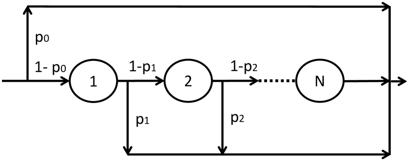
Figure 1: Cox Distribution with N stages: after staying an exponentially distributed time on a stage $i$ one has a probability $p_{i}$ of abandonment and $1-p_{i}$ to go to the next stage.

First of all let us recall that Cox topology, depicted in Figure1, can be seen as grid composed by branches, which in turn is compose by a sequence of states. In fact, in [6], the authors show that Cox topology can be reorganized equivalently as depicted Figure 2, being $q_{j}$ the routing probabilities, and the time to jump to the following state exponentially distributed. This equivalent arrangement explicit even more the fact that Cox distribution is obtained by following a sequence of states, that’s it, in order to access state $j$, we must mandatory visit all previous states $1,\ldots,j-1$.

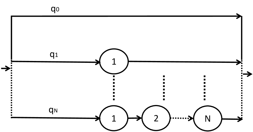
Figure 2: Equivalent Cox Distribution by reorganizing the layout of the states. Routing probabilities are $q_{0}=p_{0}$ and $q_{j}=p_{j}\prod_{k=0}^{j-1}(1-p_{k})$ for $j\in\{1,\ldots N\}$, with a convention that $p_{N}=1$.

This very interesting arrangement lead us to think that Cox structure can be made even more general, by considering independent branches with arbitrary number of states as show in Figure 3.

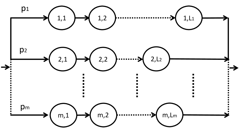
Figure 3: Generalized Cox distribution with $m$ branch routing. Each branch has $L_{j}$ states for $j=1,\ldots m$, whose routing probability is equals to $p_{j}$.

So let us explain this process a little bit more, now in terms of a service time: to generated a random service time that respect this distribution, which we call hereafter generalized Cox distribution, we first select randomly a branch $j$, $j=1,\ldots m$, with probability $p_{j}$. Once a branch is selected, the process must follow its assigned sequence of states, considering that the events that cause the transition to the adjacent states are independent and exponentially generated. For instance, let’s say that a branch $j$ is selected with probability $p_{j}$, then the process must “jump” sequentially from state $1$ till $L_{j}$, in order complete the service. The resulting distribution is really quite general. In fact, let us give an interpretation of this process in terms of a multi-class client-server system, for which we can consider different service times depending on the type of the client. In order to do this, we first consider that the jumping rate off state $kj$ denoted as $\lambda_{jk}$. So this general distribution can represent situations in which some clients are served with a negligible service time with a probability $p_{1}$ (in this case, $L_{1}=1$ and $\lambda_{11}\to\infty$, meaning, in practice, that the client pass directly through the server), other clients are served in a exponential basis with probability $p_{2}$, others obey a quite more complex way service-time distribution with probability $p_{3}$, etc.

In the sequel, we show that this generalization of the Cox distribution is really capable of representing more general distribution than the classical Cox distribution.

Property 1.

The pdf of generalized Cox distribution, expressed by Laplace transform, given by Equation 2, is more general than the one obtained by the Cox distribution, given by Equation 1.

$$f_{g}(s)=\sum_{j=1}^{m}\sum_{k=1}^{L_{j}}\frac{p_{j}\lambda_{jk}}{s+\lambda_{jk}}.$$ (2)

Proof.

To show that the presented topology , depicted Figure 3, is really more general, lets us give an example of pdf that can be realized by this topology but not with the Cox arrangement.

So we consider $m=2$, $L_{1}=L_{2}=1$, and simply denote $\lambda_{11}=\lambda_{1}$ and $\lambda_{22}=\lambda_{2}$. This consideration lead us to the following Laplace transform:

$$f_{g}(s)=\frac{p_{1}\lambda_{1}}{s+\lambda_{1}}+\frac{p_{2}\lambda_{2}}{s+\lambda_{2}}=\frac{(p_{1}\lambda_{1}+p_{2}\lambda_{2})s+\lambda_{2}\lambda_{1}}{(s+\lambda_{1})(s+\lambda_{2})},$$ (3)

using the fact that $p_{1}+p_{2}=1$.

Comparing this function with those that we can synthesize by means of a Cox topology, we can see that the only possibility to achieve the complete matching, i.e. $f_{c}(s)=f_{g}(s)$, is by trying to find routing probabilities, let’s say $q_{1}$ and $q_{2}$ for a Classical Cox topology in which $N=2$ and $q_{0}=0$. For this situation, we have:

$$f_{c}(s)=\frac{q_{1}\lambda_{1}}{s+\lambda_{1}}+\frac{q_{2}\lambda_{1}\lambda_{2}}{(s+\lambda_{1})(s+\lambda_{2})}=\frac{q_{1}\lambda_{1}s+\lambda_{2}\lambda_{1}}{(s+\lambda_{1})(s+\lambda_{2})}.$$ (4)

As a consequence, the desired equality is only ensured if $q_{1}\lambda_{1}=p_{1}\lambda_{1}+p_{2}\lambda_{2}$, which in turn is only solvable if $p_{1}+p_{2}\frac{\lambda_{2}}{\lambda_{1}}\leq 1$. Obviously, this inequality cannot be always true: take for instance $p_{1}=p_{2}=0.5$ and $\lambda_{2}=2\lambda_{1}$.

∎

Remark 1.

We have shown so far that the generalized topology depicted in Figure 3 is, in fact, even more general than the classical one. In fact, we can easily show that this distribution can represent any pdf whose Laplace transform have negative real poles. In this sense, they can be used to approximate any probability distribution with an arbitrary precision. The main advantage of such approximation is the fact that it allows us to derive analytic Markov models, with can be solved much more faster than Monte Carlo Simulation.

In the sequence, we exploit further this this topology by revisiting the classical problem of first two moments matching. We will show some new results concerning minimal achievable moments and minimal topologies.

2.1 Moment matching problem

After showing the previous generalization, let us further investigate the generalized topology in terms of moments matching. For a general pdf expressed as 2, we can show that:

$$f_{g}(s)=\sum_{k=1}^{\infty}\frac{(-1)^{k}E[T_{g}^{k}]s^{k}}{k!}.$$ (5)

So the $k^{th}$ moment of $T_{g}$ can be computed as:

$$E[T_{g}^{k}]=(-1)^{k}f_{g}^{(k)}(0),$$ (6)

in which $f_{g}^{(k)}(0)$ is the $k^{th}$ derivative of $f_{g}(s)$ evaluated at $s=0$.

In this paper, we are particularly interested in revisiting the classical problem of first and second method (e.g. mean and variance) matching. Formally our problem can be stated as:

Find the minimum number of states of topology given in Figure 3, as well as their jumping rates, ensuring that the resulting distribution has mean $\mu$ and variance $\sigma^{2}$.

This is a well known problem in literature and we want to shed more light on it, as well as presenting new results. At the end of this paper we will make comparisons with the results found in literature.

Deducing the general expression for the moments using Equation 6 is a complicated and tedious task for general pdf’s. However, for the first and second moments, we can exploit properties of our topology in order to simplify the deduction. In fact, the exponential distribution, with rate $\lambda$, has mean $1/\lambda$ and variance $1/\lambda^{2}$. So for a given branch $j$ of the process depicted in the Figure 3 we have a sum of independent random variable exponentially distributed, which we denote by $T_{j}$, whose mean and variance are respectively are given by:

$$E[T_{j}]=\sum_{k=1}^{L_{j}}1/\lambda_{jk}\\ Var[T_{j}]=\sum_{k=1}^{L_{j}}1/\lambda_{jk}^{2},$$

in which $\lambda_{jk}$ is a jump rate off the state $k$ in the branch $j$.

In order to properly write the equations, we denote hereafter $x_{jk}=1/\lambda_{jk}$ and $T_{g}$ the random variable that respect generalized Cox distribution, as depicted in Figure 3.

Recalling that for any random variable, let’s say $X$, $E[X^{2}]=E[X]^{2}+Var[X]$, we deduce that:

$$E[T_{g}]=\sum_{j=1}^{m}p_{j}(\sum_{k=1}^{L_{j}}x_{jk})$$ (7)

$$E[T_{g}^{2}]=\sum_{j=1}^{m}p_{j}[(\sum_{k=1}^{L_{j}}x_{jk})^{2}+(\sum_{i=1}^{L_{j}}x_{jk}^{2})].$$ (8)

As as result,our problem consists in finding a solution for the following system of equations, while minimizing the total number of states $(L_{1}+\ldots+L_{m})$:

$$\sum_{j=1}^{m}p_{j}(\sum_{k=1}^{L_{j}}x_{jk})=\mu;$$

$$\sum_{j=1}^{m}p_{j}[(\sum_{k=1}^{L_{j}}x_{jk})^{2}+(\sum_{i=1}^{L_{j}}x_{jk}^{2})]=\mu^{2}+\sigma^{2}.$$ (9)

Proposition 1.

For a given generalized Cox distribution, as depicted in Figure 3, the minimum value of $E[T_{g}^{2}]$, in terms of the routing probabilities and $E[T_{g}]=\mu$, is given by

$$\frac{E[T_{g}^{2}]_{mim}}{\mu^{2}\textbullet}=\frac{1}{\sum_{j=1}^{m}\frac{p_{j}L_{j}}{1+L_{j}}}.$$ (10)

Proof.

We look for a minimum value for $E[T_{g}^{2}]$, given $E[T_{g}]=\mu$, by studying the following optimization problem:

$$\underset{x_{ij}}{\text{Min}} E[T_{g}^{2}]$$ (11)

subject to $$\sum_{j=1}^{m}p_{j}(\sum_{k=1}^{L_{j}}x_{jk})-\mu=0.$$

If an optimum solution exists, the Lagrange multipliers method lead us to the following equations:

$$2p_{j}(\sum_{k=1}^{L_{j}}x_{jk})+2p_{j}x_{jk}-p_{j}\gamma=0$$

$$\sum_{j=1}^{m}p_{j}(\sum_{k=1}^{L_{j}}x_{jk})=\mu,$$

whose $\gamma$ is the Lagrange multiplier.

Without loss of generality, suppose that $p_{j}\neq 0$, then optimal solution occurs when all $x_{jk}$ are given by $\frac{\gamma}{2(1+L_{j})}$. Therefore we can show that minimum value is such that:

$$E[T_{g}^{2}]_{mim}=(\sum_{j=1}^{m}\frac{p_{j}L_{j}}{1+L_{j}})\frac{\gamma^{2}}{4}$$

$$\mu=(\sum_{j=1}^{m}\frac{p_{j}L_{j}}{1+L_{j}})\frac{\gamma}{2}.$$ (12)

As a consequence we can deduce that:

$$\frac{E[T_{g}^{2}]_{mim}}{\mu^{2}\textbullet}=\frac{1}{\sum_{j=1}^{m}\frac{p_{j}L_{j}}{1+L_{j}}}$$ (13)

∎

We can obtain an lower bound for this minimum solution by observing the following inequality:

$$\sum_{j=1}^{m}\frac{p_{j}L_{j}}{1+L_{j}}\leq\frac{L_{j^{*}}}{1+L_{j^{*}}}$$

in which $j^{*}=\underset{j}{Arg}~{}Max\frac{L_{j}}{1+L_{j}}$ . Therefore:

$$\frac{E[T_{g}^{2}]_{mim}}{\mu^{2}\textbullet}\geq\frac{1+L_{j^{*}}}{L_{j^{*}}}=1+\frac{1}{L_{j^{*}}}.$$ (14)

So far we have found a minimum value for the second moment for the Generalized Cox Topology 3, given the mean and the routing probabilities. We have as well establish an interesting lower bound, based on the number of states, given by Inequality 14.

Remark 2.

We remark that the lower bound 14 was presented before using a completely different approach in [11], as corollary of a more general result presented before in [3]. However in those papers, the authors do not concern in minimizing second moment, given the mean, as we did, and do not present a general expression for the minimum value as show in Equation 10.

2.2 Minimal Structures for First and Second Moment Matching

The result 14 ensures that the ratio variance /mean of the distribution (we recall that$Var[T_{g}^{2}]=E[T_{g}^{2}]-\mu^{2}$), can not be smaller than the one obtained for the longest branch. So hereafter we focus on what we can achieve by using just one branch with $N$ states. The obtained distribution in this case is known as Hypoexponential (or generalized Erlang) distribution, and it is depicted in Figure 4.

Figure 4: A particular case: Hypoexponential (or generalized Erlang) distribution

In this particular situation, the minimum value for the second moment, is given by Equation 10:

$$\frac{E[T_{g}^{2}]_{mim}}{\mu^{2}\textbullet}=\frac{1}{\frac{N}{1+N}}=1+\frac{1}{N}.$$ (15)

It is well known that this minimum value is achieve for a Erlang Distribuition, with $x_{i}=\mu/N$ if $\frac{\sigma^{2}}{\mu^{2}}=\frac{1}{N}$. So let us investigate more general situations in which this equality is not true. In this sense, our moment matching problem is simplified as solving the following pair of equation for a minimum $N$:

$$\sum_{i=1}^{N}x_{i}=\mu$$

$$\sum_{i=1}^{N}x_{i}^{2}=\sigma^{2}$$ (16)

First, we must observe that triangular and internal product inequalities (Cauchy-Schwartz Inequality) lead to:

$$\frac{(\sum_{i=1}^{N}x_{i})^{2}}{N}\leq\sum_{i=1}^{N}x_{i}^{2}\leq(\sum_{i=1}^{N}x_{i})^{2}$$ (17)

As a result, provided that a solutions exists, they are all such that:

$$\frac{\mu^{2}}{N}\leq\sum_{i=1}^{N}x_{i}^{2}\leq\mu^{2}$$ (18)

So the number of stages $N$ must satisfies:

$$\frac{\mu^{2}}{N}\leq\sigma^{2}\rightarrow N\geq\frac{\mu^{2}}{\sigma^{2}}.$$ (19)

Since $N$ is an integer, its smallest possible value is $N=\lceil\frac{\mu^{2}}{\sigma^{2}}\rceil$.

Keeping in mind those observations, we present a solution for the system of equations 16. First we observe that if $\frac{\mu^{2}}{\sigma^{2}}=1$, the solution is trivial, with only one state, that is $N=1$. So let us concentrate our attention in the situations for which $\lceil\frac{\mu^{2}}{\sigma^{2}}\rceil\geq 2$.

Proposition 2 (Almost Erlang Solution).

If $\lceil\frac{\mu^{2}}{\sigma^{2}}\rceil\geq 2$, a solution for the system of equations 16 is given by:

$$x_{j}=\frac{\mu}{N}-\frac{\alpha_{N}}{\sqrt{(N-1)}}~{}~{}(1\leq j\leq N-1),$$ (20)

and

$$x_{N}=\frac{\mu}{N}+\sqrt{(N-1)}\alpha_{N}.$$ (21)

being $N=\lceil\frac{\mu^{2}}{\sigma^{2}}\rceil$, $\alpha_{N}=\frac{\sqrt{N\sigma^{2}-\mu^{2}}}{N}$.

Proof.

By denoting $x_{j}=y$ $(1\leq j\leq N-1)$ and $x_{N}=z$, it is straightforward to check that :

$$\left\{\begin{matrix}(N-1)y+z=\mu,&\\ (N-1)y^{2}+z^{2}=\sigma^{2},&\end{matrix}\right.$$ (22)

which obviously ensure 16.

∎

Corollary 1 (Erlang Solution).

In particular, If $\frac{\mu^{2}}{\sigma^{2}}=N$, a solution is given by $x_{i}=\frac{\mu}{N}$.

Proof.

In this situation, we can verify that $\alpha_{N}=0$, ensuring the claimed result.

∎

Remark 3.

We remark that the result given by Proposition 2 is the same as the one obtained by the Erlang Distribution if $\frac{\mu^{2}}{\sigma^{2}}=N$. If it is not the case, it is important to recall that Erlang distribution does not ensure the first two moments matching. However we prove that is still possible to achieve the matching by appropriately changing the rates of stages.

So far, we have established that if $\sigma^{2}\leq\mu^{2}$, the minimum number of states is given by $N=\lceil\frac{\mu^{2}}{\sigma^{2}}\rceil$, being the means between states provided by Proposition 2.

It remains to solve the cases for which if $\sigma^{2}$ is strictly greater than $\mu^{2}$. We address this problem by considering two states and two routing probability, as depicted in Figure 5. This configuration, lead us to an Hyperexponential distribution. In fact, Equation 10 ensures that:

$$\frac{E[T_{g}^{2}]_{mim}}{\mu^{2}\textbullet}=\frac{1}{\frac{p}{1+1}+\frac{1-p}{1+1}}=2,$$ (23)

which is compatible with our aim to have $E[T_{g}^{2}]=\sigma^{2}+\mu^{2}\geq 2\mu^{2}.$

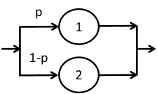
Figure 5: A particular case: Hyper-exponential Distribution

For this particular structure, the general system of equation 9 is reduced to:

$$E[T_{g}]=px_{1}+(1-p)x_{2}=\mu,$$ (24)

$$E[T_{g}^{2}]=2px_{1}^{2}+2(1-p)x_{2}^{2}=\sigma^{2}+\mu^{2}.$$ (25)

Considering, without loss of generality that $x_{1}\geq x_{2}$, we solve the system of equation. The obtained solutions are given by:

$$x_{1}=\mu(1+\frac{\alpha}{p}),$$ (26)

$$x_{2}=\mu(1-\frac{\alpha}{1-p}).$$ (27)

being $0<p\leq\frac{2}{1+C_{v}^{2}}$, $\alpha=\sqrt{\frac{p(1-p)(C_{v}^{2}-1)}{2}}$ and $C_{v}$ the coefficient of variation, i.e $C_{v}=\frac{\sigma}{\mu}$. So the simplest topology to ensure the desired results is given by choosing $p=p_{max}=\frac{2}{1+C_{v}^{2}}$, leading to $x_{1}=\mu\frac{C_{v}^{2}+1}{2}$ and $x_{2}=0$. This topology, which has only one state, is shown in Figure 6.

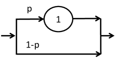
Figure 6: The simplest form: Hyper-exponential Distribution

Remark 4.

An interpretation of the resulting distribution for this topology, in terms of service time, is the following: with probability $p$, some clients are served with exponentially distributed service time with mean $x_{1}$, while others are served with negligible service mean with probability $(1-p)$.

Complete Method Summary

• if $\sigma^{2}<\mu^{2}$: $N=\lceil\frac{\mu^{2}}{\sigma^{2}}\rceil$
  

  

  $$\frac{1}{\lambda_{j}} = x_{j}=\frac{\mu}{N}-\frac{\alpha_{N}}{\sqrt{(N-1)}}~{}~{}~{}(1\leq j\leq N-1),$$

  $$\frac{1}{\lambda_{N}} = \frac{\mu}{N}+\sqrt{(N-1)}\alpha_{N}.$$

  being $\alpha_{N}=\frac{\sqrt{N\sigma^{2}-\mu^{2}}}{N}$ .
  

• if $\sigma^{2}\geq\mu^{2}$:

  

  $$p=\frac{2}{1+(\frac{\sigma}{\mu})^{2}},~{}~{}~{}~{}~{}~{}x_{1}=\mu\frac{(\frac{\sigma}{\mu})^{2}+1}{2}.$$

2.3 Comparison with other results

The so classical approaches to solve the model matching problem are presented in [24] and [21]. In [24] the authors presents two topologies which are particular cases of the general Cox distribution presented in Figure 3: for $\sigma^{2}\leq\mu^{2}$, the resulting structure is not minimal since it uses the same number of states, but with the need of a routing probability after the first state; on the other hand if $\sigma^{2}>\mu^{2}$, the topology is not minimal as well since it uses two states with means $x_{1}=\frac{\mu}{2p}$ and $x_{2}=\frac{\mu}{2(1-p)}$, leading to a particular routing probability $p=\frac{C_{v}^{2}+1-\sqrt{C_{v}^{4}-1}}{2(C_{v}^{2}+1)}$. In [21], a particular Cox topology is presented for solving the problem for any coefficient of variation. For the cases in which $\sigma^{2}<\mu^{2}$, the resulting structure is the same as proposed by [24]; if $\sigma^{2}>\mu^{2}$, the structure presents two states with a routing probability after the first state, which is not minimal as well.

3 Application: Timing Sthocastic Discrete-Event Models

The generalized Cox distribution can be used for timing events in discrete-event system in a quite general way. If we are interested in developing analytic model, we can observe that the topology depicted in Figure 3 can be rewritten as continuous-time Markov chain as show in Figure 7, whose states I and E represent respectively and event activation and E its effectively occurrence, being value $\lambda$ an infinity (huge) rate introduced in order to simulate the routing mechanism. In practice, in order to have a good approximation this rate must be chosen much lager than the others present in the chain.

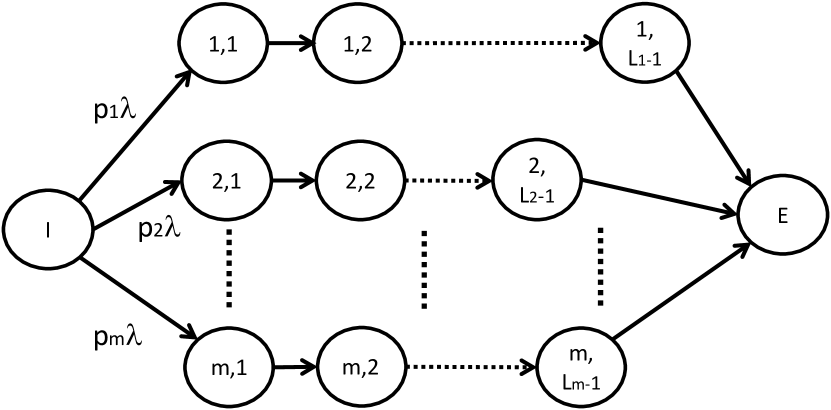
Figure 7: Generalized Cox distribution as an absorbing continuous Markov Chain, in which states I and E represent respectively the activation and the occurrence of an event.

So between states “S” and “E” we have inserted several intermediary states whose transitions operates with markovian jumps in such a way that the “ big jump” between “S” and “E” respects the desired distribution. In practical situations, minimal topology can be derived by matching the mean and variance of the collected data as show in previous section.

On the other hand, if we are interested computer-simulation models, the generalized Cox distribution samples can be generated from uniform a distribution using the inverse transform method. Suppose that we want to generate a random event-time (for stochastic automata) or a random delay (for stochastic Petri nets), let’s say $T_{g}$. If this random variable is purely exponential with rate $\lambda$, it’s well known that it can be generated from an uniform random variable $U\in[0~{}1]$ as:

$$T_{g}=-\dfrac{1}{\lambda}\ln U,$$ (29)

ensuring, obviously, that $U\neq 0$.

If $T_{g}$ respects the generalized Cox-distribution, as depicted in Figure 3, it can be generated by following simple steps:

• Sample  $M\in\{1,\ldots m\}$   s.t.  $P[M=j]=p_{j}$;
  

• Sample $U_{k}\in[0~{}~{}1],~{}\forall~{}k\in\{1,\ldots L_{M}\}$;
  

• Compute $T_{g}=-\sum_{k=1}^{L_{M}}\dfrac{1}{\lambda_{Mk}}\ln U_{k}$,

whose $U_{k}$ are uniformly distributed random variables in $[0~{}1]$ such that $U_{k}\neq 0$.

In the same way as for analytic models, minimal topology can be derived by matching the mean and variance of the collected data as show in previous section.

4 Conclusion

With this paper we have expected to contribute to the fundamental problem of stochastic event timimg by means of markovian jumps, which has a direct impact on the developing analytic and simulation models for Stochastic Systems. To this end we have revisited the classical Cox topology and its equivalent representation, then we derive an even more general topology, capable of representing quite complex distributions. From this general distribution, we revisited and reformulated the problem of moments matching in quest of minimal topologies. First we have established an expression for the minimum value of the second moment, given the first one, as well as a lower bound for it. In the sequence, we have presented minimal structures for the first two moments matching problem, which are simpler than the ones found in literature. As quite direct application of the results, we show how to generate random events for stochastic discrete-event for analytic and simulation purposes. For future works, we suggest further investigation concerning higher order moments matching or other metrics concerning transfer function matching.

References

- [1] M. Ades, P. E. Caines, and R. P. Malhame. Stochastic optimal control under poisson-distributed observations. IEEE Trans. on Automatic Control, 45(1):3–13, Jan. 2000.
- [2] P. Agarwal, D. E. Thomas, and A. Kumar. Security analysis of lte/sae networks under de-synchronization attack for hyper-erlang distributed residence time. IEEE Communication Letters, 21(5):1055–1058, May 2017.
- [3] D. Aldous and L. Shepp. The least variable phasetype distribution is erlang. Communications in Statistics Stochastic Models, 3(3):467–473, Dec. 1987.
- [4] R. Ammoura, E. Leclercq, E. Sanlaville, and D. Lefebvre. Fault prognosis of timed stochastic discrete event systems with bounded estimation error. Automatica, 82:35–41, August 2017.
- [5] L. R. Arnaut. Pulse jitter, delay spread, and doppler shift in mode-stirred reverberation. IEEE Trans on Eletrom. Compatibility, 58(6):1717–1727, Dec. 2016.
- [6] R. Augustin and K. J. Buscher. Characteristics of the cox-distribution. ACM SIGMETRICS Performance Evaluation Review, 12(1):22–31, 1982.
- [7] G. Bolch, S. Greiner, H. de Meer, and K. S. Triverdi. Queueing Networks and Markov Chains: Modeling and Performance Evaluation with Computer Science Applications. Wiley-Blackwell, 2006.
- [8] A. Brandwajn and T. Begin. First-come-first-served queues with multiple servers and customer classes. Performance Evaluation, 130:51–63, 2019.
- [9] A. Busic, B. Gaujal, G. Gorgoz, and J.-M. Vincentz. Psi2 : Envelope perfect sampling of non monotone systems. In Seventh International Conference on the Quantitative Evaluation of Systems, pages 83–84, Williamsburg, VA, USA, 2010.
- [10] C. G. Cassandras and S. Lafortune. Introduction to Discrete Event Systems. Springer US, 2008.
- [11] C. Commault and S. Mocanu. Phase-type distributions and representations: Some results and open problems for system theory. International Journal of Control, 76(6):566–580, 2003.
- [12] D. R. Cox. A use of complex probabilities in the theory of stochastic processes. Mathematical Proceedings of the Cambridge Philosophical Society, 51:313–314, 1955.
- [13] Qihong Duan and Junrong Liu. Modelling a bathtub-shaped failure rateby a coxian distribution. IEEE Trans. on Reliability, 65(2):878–885, 2016.
- [14] Y. Fang and I. Chlamtac. Teletraffic analysis and mobility modeling of pcs networks. IEEE Trans. on Communications, 47(7):1062–1072, 1999.
- [15] S. Jafari and K. Savla. On the optimal control of a class of degradable systems modeled by semi-markov jump linear systems. In IEEE 56th Annual Conference on Decision and Control (CDC), pages 1–6, Melbourne, Australia, 2017.
- [16] A. D. Khomonenko, A. I. Danilov, P. V. Gerasimenko, and A. A. Danilov. Nonstationary software testing models with cox distribution for fault resolution duration. In XIX IEEE International Conference on Soft Computing and Measurements (SCM), pages 209–2012, St. Petersburg, Russia, 2016.
- [17] Y. Chen L. Chen and Z. Pang. Dynamic pricing and inventory control in a make-to-stock queue with information on the production status. IEEE Trans. on Automation Science and Engineering, 8(2):361–373, April 2011.
- [18] S. Lagershausen. Markov-chain model and algorithmic procedure for the performance analysis of closed cyclic queues. Performance Evaluation, 90:1–17, 2015.
- [19] F. Li, L. Wua, P. Shi, and C.-C. Limb. State estimation and sliding mode control for semi-markovian jump systems with mismatched uncertainties. Automatica (Oxford), 51:385–393, January 2015.
- [20] Z. Li and Q. Liang. Capacity optimization in heterogeneous home area networks with application to smart grid. IEEE Trans. on Vehicular Technology, 65(2):699–706, 2016.
- [21] R. A. Marie. Calculating equilibrium probabilities for lambda(n)/ck/1/n queues. ACM SIGMETRICS Performance Evaluation Review, 9:117–125, 1980.
- [22] T. Osogami and M. Harchol-Balter. Closed form solutions for mapping general distributions to quasi-minimal ph distributions. Performance Evaluation, 63(4):524–552, 2006.
- [23] R. Rollins, A. H. Marshall E. McLoone, and S. Chamney. Discrete conditional phase-type model utilising a multiclass support vector machine for the prediction of retinopathy of prematurity. In IEEE 28th International Symposium on Computer-Based Medical Systems, pages 1–6, Brazil, June 2015.
- [24] C. H. Sauer and K. M. Chandy. Approximate analysis of central server models. IBM Journal of Research and Development, 19:301–313, 1975.
- [25] Bo Shen, H. Tan, Z. Wang, and T. Huang. Quantized/saturated control for sampled-data systems under noisy sampling intervals: A confluent vandermonde matrix approach. IEEE Trans. on Automatic Control, 62(9):4753–4759, September 2017.
- [26] M. Soltani and A. Singh. Moment-based analysis of stochastic hybrid systems with renewal transitions. Automatica (Oxford), 84:62–69, October 2017.
- [27] Q. Xu, L. Xing, Z. Tian, Y. Zhao, L. Chen, L. Shi, and Y. Huang. Statistical distribution of the enhanced backscatter coefficient in reverberation chamber. IEEE Trans. on Antennas and Propagation, 66(4):2161–2164, 2018.