Continuous Adaptation for Interactive Object Segmentation by Learning from Corrections

Abstract

In interactive object segmentation a user collaborates with a computer vision model to segment an object. Recent works employ convolutional neural networks for this task: Given an image and a set of corrections made by the user as input, they output a segmentation mask. These approaches achieve strong performance by training on large datasets but they keep the model parameters unchanged at test time. Instead, we recognize that user corrections can serve as sparse training examples and we propose a method that capitalizes on that idea to update the model parameters on-the-fly to the data at hand. Our approach enables the adaptation to a particular object and its background, to distributions shifts in a test set, to specific object classes, and even to large domain changes, where the imaging modality changes between training and testing. We perform extensive experiments on 8 diverse datasets and show: Compared to a model with frozen parameters, our method reduces the required corrections (i) by 9%-30% when distribution shifts are small between training and testing; (ii) by 12%-44% when specializing to a specific class; (iii) and by 60% and 77% when we completely change domain between training and testing.

1 Introduction

In interactive object segmentation a human collaborates with a computer vision model to segment an object of interest [12, 49, 56, 11]. The process iteratively alternates between the user providing corrections on the current segmentation and the model refining the segmentation based on these corrections. The objective of the model is to infer an accurate segmentation mask from as few user corrections as possible (typically point clicks [8, 16] or strokes [49, 24] on mislabeled pixels). This enables fast and accurate object segmentation, which is indispensable for image editing [2] and collecting ground-truth segmentation masks at scale [11].

\begin{overpic}[trim=42.67912pt 14.22636pt 0.0pt 0.0pt,clip,width=368.57964pt]{figures/splash_figure.pdf} \put(-35.0,350.0){\makebox(0.0,0.0)[]{\rotatebox{90.0}{{F}rozen model{}~{}\cite[cite]{[\@@bibref{}{mahadevan18bmvc}{}{}]}}}} \put(-35.0,100.0){\makebox(0.0,0.0)[]{\rotatebox{90.0}{{Ours}}}} \end{overpic}

Figure 1: Example results for a frozen model (top) and our adaptive methods (bottom). A frozen model performs poorly when foreground and background share similar appearance (left), when it is used to segment new object classes absent in the training set (center, donut class), or when the model is tested on a different image domain (aerial) than it is trained on (consumer) (right). By using corrections to adapt the model parameters to a specific test image, or to the test image sequence, our method substantially improves segmentation quality. The input is four corrections in all cases shown.

Current state-of-the-art methods train a convolutional neural network (CNN) which takes an image and user corrections as input and predicts a foreground / background segmentation [56, 35, 10, 38, 33, 11, 29]. At test time, the model parameters are frozen and corrections are only used as additional input to guide the model predictions. But in fact, user corrections directly specify the ground-truth labelling of the corrected pixels. In this paper we capitalize on this observation: we treat user corrections as training examples to adapt our model on-the-fly. We use these user corrections in two ways: (1) in single image adaptation we iteratively adapt model parameters to one specific object in an image, given the corrections produced while segmenting that object; (2) in image sequence adaptation we adapt model parameters to a sequence of images with an online method, given the set of corrections produced on these images. Each of these leads to distinct advantages over using a frozen model:

During single image adaptation our model learns the specific appearance of the current object instance and the surrounding background. This allows the model to adapt even to subtle differences between foreground and background for that specific example. This is necessary when the object to be segmented has similar color to the background (Fig. 1, 1st column), has blurry object boundaries, or low contrast. In addition, a frozen model can sometimes ignore the user corrections and overrule them in its next prediction. We avoid this undesired behavior by updating the model parameters until its predictions respect the user corrections.

During image sequence adaptation we continuously adapt the model to a sequence of segmentation tasks. Through this, the model parameters are optimized to the image and class distribution in these tasks, which may consist of different types of images or a set of new classes which are unseen during training. An important case of this is specializing the model for segmenting objects of a single class. This is useful for collecting many examples in high-precision domains, such as pedestrians for self-driving car applications. Fig. 1, middle column shows an example of specializing to the single, unseen class donut. Furthermore, an important property of image sequence adaptation is that it enables us to handle large domain changes, where the imaging modality changes dramatically between training and testing. We demonstrate this by training on consumer photos while testing on medical and aerial images (Fig. 1, right column).

Naturally, single image adaptation and image sequence adaptation can be used jointly, leading to a method that combines their advantages.

In summary: Our innovative idea of treating user corrections as training examples allows to update the parameters of an interactive segmentation model at test time. To update the parameters we propose a practical online adaptation method. Our method operates on sparse corrections, balances adaptation vs. retaining old knowledge and can be applied to any CNN-based interactive segmentation model. We perform extensive experiments on 8 diverse datasets and show: Compared to a model with frozen parameters, our method reduces the required corrections (i) by 9%-30% when distribution shifts are small between training and testing; (ii) by 12%-44% when specializing to a specific class; (iii) and by 60% and 77% when we completely change domain between training and testing. (iv) Finally, we evaluate on four standard datasets where distribution shifts between training and testing are minimal. Nevertheless, our method did set a new state-of-the-art on all of them, when it was initially released [32].

2 Related Work

Interactive Object Segmentation. Traditional methods approach interactive segmentation via energy minimization on a graph defined over pixels [12, 49, 7, 24, 44]. User inputs are used to create an image-specific appearance model based on low-level features (e.g. color), which is then used to predict foreground and background probabilities. A pairwise smoothness term between neighboring pixels encourages regular segmentation outputs. Hence these classical methods are based on a weak appearance model which is specialized to one specific image.

Recent methods rely on Convolutional Neural Networks (CNNs) to interactively produce a segmentation mask [56, 35, 10, 38, 33, 16, 28, 29, 3]. These methods take the image and user corrections (transformed into a guidance map) as input and map them to foreground and background probabilities. This mapping is optimized over a training dataset and remains frozen at test time. Hence these models have a strong appearance model but it is not optimized for the test image or dataset at hand.

Our method combines the advantages of traditional and recent approaches: We use a CNN to learn a strong initial appearance model from a training set. During segmentation of a new test image, we adapt the model to it. It thus learns an appearance model specifically for that image. Furthermore, we also continuously adapt the model to the new image and class distribution of the test set, which may be significantly different from the one the model is originally trained on.

Gradient Descent at test time. Several methods iteratively minimize a loss at test time. The concurrent work of [54] uses self-supervision to adapt the feature extractor of a multi-tasking model to the test distribution. Instead, we directly adapt the full model by minimizing the task loss. Others iteratively update the inputs of a model [23, 25, 29],  e.g. for style transfer [23]. In the domain of interactive segmentation, [29] updates the guidance map which encodes the user corrections and is input to the model. [52] made this idea more computationally efficient by updating intermediate feature activations, rather than the guidance maps. Instead, our method updates the model parameters, making it more general and allowing it to adapt to individual images as well as sequences.

In-domain Fine-Tuning. In other applications it is common practice to fine-tune on in-domain data when transferring a model to a new domain [13, 42, 55, 61]. For example, when supervision for the first frame of a test video is available [43, 55, 13], or after annotating a subset of an image dataset [42, 61]. In interactive segmentation the only existing attempt is [1], which performs polygon annotation [15, 1, 37]. However, it does not consider adapting to a particular image; their process to fine-tune on a dataset involves 3 different models, so they do it only a few times per dataset; they cannot directly train on user corrections, only on complete masks from previous images; finally, they require a bounding box on the object as input.

Few-shot and Continual Learning. Our method automatically adapts to distribution shifts and domain changes. It performs domain adaptation from limited supervision, similar to few-shot learning [46, 22, 51, 45]. It also relates to continual learning [47, 21], except that the output label space of the classifier is fixed. As in other works, our method needs to balance between preserving existing knowledge and adapting to new data. This is often done by fine-tuning on new tasks while discouraging large changes in the network parameters, either by penalizing changes to important parameters [31, 58, 5, 6] or changing predictions of the model on old tasks [34, 50, 41]. Alternatively, some training data of the old task is kept and the model is trained on a mixture of the old and new task data [47, 9].

3 Method

We adopt a typical interactive object segmentation process [12, 56, 38, 33, 11, 29]: the model is given an image and makes an initial foreground / background prediction for every pixel. The prediction is then overlaid on the image and presented to the user, who is asked to make a correction. The user clicks on a single pixel to mark that it was incorrectly predicted to be foreground instead of background or vice versa. The model then updates the predicted segmentation based on all corrections received so far. This process iterates until the segmentation reaches a desired quality level.

We start by describing the model we build on (Sec. 3.1). Then, we describe our core contribution: treating user corrections as training examples to adapt the model on-the-fly at test-time (Sec. 3.2). Lastly, we describe how we simulate user corrections to train and test our method (Sec. 3.3).

3.1 Interactive Segmentation Model

As the basis of our approach, we use a strong re-implementation of [38], an interactive segmentation model based on a convolutional neural network. The model takes an RGB image and the user corrections as input and produces a segmentation mask. As in [11] we encode the position of user corrections by placing binary disks into a guidance map. This map has the same resolution as the image and consists of two channels (one channel for foreground and one for background corrections). The guidance map is concatenated with the RGB image to form a 5-channel map $\boldsymbol{\mathbf{x}}$ which is provided as input to the network.

We use DeepLabV3+ [17] as our network architecture, which has demonstrated good performance on semantic segmentation. However, we note that our method does not depend on a specific architecture and can be used with others as well.

For training the model we need a training dataset $\mathcal{D}$ with ground-truth object segmentations, as well as user corrections which we simulate as in [38] (Sec. 3.3). We train the model using the cross-entropy loss over all pixels in an image:

$$\mathcal{L}_{\mathrm{CE}}(\boldsymbol{\mathbf{x}},\boldsymbol{\mathbf{y}};\boldsymbol{\mathbf{\theta}})=\frac{1}{|\boldsymbol{\mathbf{y}}|}\{-\boldsymbol{\mathbf{y}}\log\boldsymbol{\mathbf{f}}(\boldsymbol{\mathbf{x}};\boldsymbol{\mathbf{\theta}})-(1-\boldsymbol{\mathbf{y}})\log(1-\boldsymbol{\mathbf{f}}(\boldsymbol{\mathbf{x}};\boldsymbol{\mathbf{\theta}}))\}$$ (1)

where $\boldsymbol{\mathbf{x}}$ is the 5-channel input defined above (image plus guidance maps), $\boldsymbol{\mathbf{y}}\in\{0,1\}^{H\times W}$ are the pixel labels of the ground-truth object segmentations, and $\boldsymbol{\mathbf{f}}(\boldsymbol{\mathbf{x}};\boldsymbol{\mathbf{\theta}})$ represents the mapping of the convolutional network parameterized by $\boldsymbol{\mathbf{\theta}}$. $|\cdot|$ denotes the $l_{1}$ norm.

We produce the initial parameters $\boldsymbol{\mathbf{\theta}}^{*}$ of the segmentation model by minimizing $\sum_{(\boldsymbol{\mathbf{x}}_{i},\boldsymbol{\mathbf{y}}_{i})\in\mathcal{D}}\mathcal{L}_{\mathrm{CE}}(\boldsymbol{\mathbf{x}}_{i},\boldsymbol{\mathbf{y}}_{i};\boldsymbol{\mathbf{\theta}})$ over the training set using stochastic gradient descent.

3.2 Learning from Corrections at Test-Time

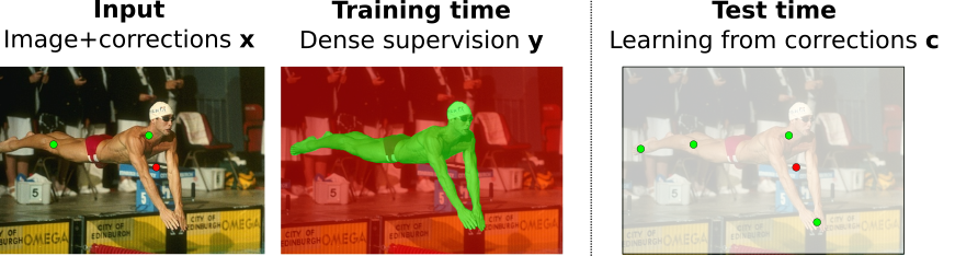
Figure 2: Corrections as training examples. For learning the initial model parameters, full supervision is available, allowing to compute a loss over all the pixels in the image. At test time, the user provides sparse supervision in the form of corrections. We use these to adapt the model parameters.

Previous interactive object segmentation methods do not treat corrections as training examples. Thus, the model parameters remain unchanged/frozen at test time [56, 10, 38, 33, 11, 29] and corrections are only used as inputs to guide the predictions. Instead, we treat corrections as ground-truth labels to adapt the model at test time. We achieve this by minimizing the generalized cross-entropy loss over the corrected pixels:

$$\mathcal{L}_{\mathrm{GCE}}(\boldsymbol{\mathbf{x}},\boldsymbol{\mathbf{c}};\boldsymbol{\mathbf{\theta}})=\frac{\boldsymbol{\mathbf{1}}[{\scriptstyle\boldsymbol{\mathbf{c}}\neq-1}]^{T}}{|\boldsymbol{\mathbf{1}}[{\scriptstyle\boldsymbol{\mathbf{c}}\neq-1}]|}\bigg{\{}-\boldsymbol{\mathbf{c}}\log\boldsymbol{\mathbf{f}}(\boldsymbol{\mathbf{x}};\boldsymbol{\mathbf{\theta}})-(1-\boldsymbol{\mathbf{c}})\log\left(1-\boldsymbol{\mathbf{f}}\left(\boldsymbol{\mathbf{x}};\boldsymbol{\mathbf{\theta}}\right)\right)\bigg{\}}$$ (2)

where $\boldsymbol{\mathbf{1}}$ is an indicator function and $\boldsymbol{\mathbf{c}}$ is a vector of values $\{1,0,-1\}$, indicating what pixels were corrected to what label. Pixels that were corrected to be positive are set to $1$ and negative pixels to $0$. The remaining ones are set to $-1$, so that they are ignored in the loss. As there are very few corrections available at test time, this loss is computed over a sparse set of pixels. This is in contrast to the initial training which had supervision at every pixel (Sec. 3.1). We illustrate the contrast between the two forms of supervision in Fig. 2.

Dealing with label sparsity. In practice, corrections $\boldsymbol{\mathbf{c}}$ are extremely sparse and consist of just a handful of scattered points (Fig. 3). Hence, they offer limited information on the spatial extent of objects and special care needs to be taken to make this form of supervision useful in practice. As our model is initially trained with full supervision, it has learned strong shape priors. Thus, we propose two auxiliary losses to prevent forgetting these priors as the model is adapted. First, we regularize the model by treating the initial mask prediction $\boldsymbol{\mathbf{p}}$ as ground-truth and making it a target in the cross-entropy loss, i.e. $\mathcal{L}_{\mathrm{CE}}(\boldsymbol{\mathbf{x}},\boldsymbol{\mathbf{p}};\boldsymbol{\mathbf{\theta}})$. This prevents the model from focusing only on the user corrections while forgetting the initially good predictions on pixels for which no corrections were given.

Second, inspired by methods for class-incremental learning [31, 58, 5], we minimize unnecessary changes to the network parameters to prevent it from forgetting crucial patterns learned on the initial training set. Specifically, we add a cost for changing important network parameters:

$$\mathcal{L}_{\mathrm{F}}(\boldsymbol{\mathbf{\theta}})=\boldsymbol{\mathbf{\Omega}}^{T}\left(\boldsymbol{\mathbf{\theta}}-\boldsymbol{\mathbf{\theta^{*}}}\right)^{\odot 2}$$ (3)

where $\boldsymbol{\mathbf{\theta^{*}}}$ are the initial model parameters, $\boldsymbol{\mathbf{\theta}}$ are the updated parameters and $\boldsymbol{\mathbf{\Omega}}$ is the importance of each parameter. $(\cdot)^{\odot 2}$ is the element-wise square (Hadamard square). Intuitively, this loss penalizes changing the network parameters away from their initial values, where the penalty is higher for important parameters. We compute $\boldsymbol{\mathbf{\Omega}}$ using Memory-Aware Synapses (MAS) [5], which estimates importance based on how much changes to the parameters affect the prediction of the model.

Combined loss. Our full method uses a linear combination of the above losses:

$$\mathcal{L}_{\mathrm{ADAPT}}(\boldsymbol{\mathbf{x}},\boldsymbol{\mathbf{p}},\boldsymbol{\mathbf{c}};\boldsymbol{\mathbf{\theta}})=\lambda\mathcal{L}_{\mathrm{GCE}}(\boldsymbol{\mathbf{x}},\boldsymbol{\mathbf{c}};\boldsymbol{\mathbf{\theta}})+(1-\lambda)\mathcal{L}_{\mathrm{GCE}}(\boldsymbol{\mathbf{x}},\boldsymbol{\mathbf{p}};\boldsymbol{\mathbf{\theta}})+\gamma\mathcal{L}_{\mathrm{F}}(\boldsymbol{\mathbf{\theta}})$$ (4)

where $\lambda$ balances the importance of the user corrections vs. the predicted mask, and $\gamma$ defines the strength of parameter regularization. Next, we introduce single image adaptation and image sequence adaptation, which both minimize Eq. (4). Their difference lies in how the model parameters $\boldsymbol{\mathbf{\theta}}$ are updated: individually for each object or over a sequence.

3.2.1 Adapting to a single image.

We adapt the segmentation model to a particular object in an image by training on the click corrections. We start from the segmentation model with parameters $\boldsymbol{\mathbf{\theta^{*}}}$ fit to the initial training set (Sec. 3.1). Then we update them by running several gradient descent steps to minimize our combined loss Eq. (4) every time the user makes a correction (Algo. in supp. material). We choose the learning rate and the number of update steps such that the updated model adheres to the user corrections. This effectively turns corrections into constraints. This process results in a segmentation mask $\boldsymbol{\mathbf{p}}$, predicted using the updated parameters $\boldsymbol{\mathbf{\theta}}$.

Adapting the model to the current test image brings two core advantages. First, it learns about the specific appearance of the object and background in the current image. Hence corrections have a larger impact and can also improve the segmentation of distant image regions which have similar appearance. The model can also adapt to low-level photometric properties of this image, such as overall illumination, blur, and noise, which results in better segmentation in general. Second, our adaptation step makes the corrections effectively hard constraints, so the model will preserve the corrected labeling in later iterations too.

This adaptation is done for each object separately, and the updated $\boldsymbol{\mathbf{\theta}}$ is discarded once an object is segmented.

3.2.2 Adapting to an image sequence.

Here we describe how to continuously adapt the segmentation model to a sequence of test images using an online algorithm. Again, we start from the model parameters $\boldsymbol{\mathbf{\theta^{*}}}$ fit to the initial training set (Sec. 3.1). When the first test image arrives, we perform interactive segmentation using these initial parameters. Then, after segmenting each image $I_{t}=(\boldsymbol{\mathbf{x}}_{t},\boldsymbol{\mathbf{c}}_{t})$, the model parameters are updated to $\boldsymbol{\mathbf{\theta}}_{t+1}$ by doing a single gradient descent step to minimize Eq. (4) for that image. Thereby we subsample the corrections in the guidance maps to avoid trivial solutions (predict the corrections given the corrections themselves, see supp. material). The updated model parameters are used to segment the next image $I_{t+1}$.

Through the method described above our model adapts to the whole test image sequence, but does so gradually, as objects are segmented in sequence. As a consequence, this process is fast, does not require storing a growing number of images, and can be used in a online setting. In this fashion it can adapt to changing appearance properties, adapt to unseen classes, and specialize to one particular class. It can even adapt to radically different image domains as we demonstrate in Sec. 4.3.

3.2.3 Combined adaptation.

For a test image $I_{t}$, we segment the object using single image adaptation (Algo. in supp. material). After segmenting a test image, we gather all corrections provided for that image and apply a image sequence adaptation step to update the model parameters from $\boldsymbol{\mathbf{\theta}}_{t}$ to $\boldsymbol{\mathbf{\theta}}_{t+1}$. At the next image, the image adaptation process will thus start from parameters $\boldsymbol{\mathbf{\theta}}_{t+1}$ better suited for the test sequence. This combination allows to leverage the distinct advantages of the two types of adaptation.

3.3 Simulating user corrections

To train and test our method we rely on simulated user corrections, as is common practice [56, 35, 10, 38, 33, 29].

Test-time corrections. When interactively segmenting an object, the user clicks on a mistake in the predicted segmentation. To simulate this we follow [56, 10, 38], which assume that the user clicks on the largest error region. We obtain this error region by comparing the model predictions with the ground-truth and select its center pixel.

Train-time corrections. Ideally one wants to train with the same user model that is used at test-time. To make this computationally feasible, we train the model in two stages as in [38]. First, we sample corrections using ground-truth segmentations [10, 29, 33, 35, 56]. Positive user corrections are sampled uniformly at random on the object. Negative user corrections are sampled according to three strategies: (1) uniformly at random from pixels around the object, (2) uniformly at random on other objects, and (3) uniformly around the object. We use these corrections to train the model until convergence. Then, we continue training by iteratively sampling corrections following [38]. For each image we keep a set of user corrections $\boldsymbol{\mathbf{c}}$. Given $\boldsymbol{\mathbf{c}}$ we predict a segmentation mask, simulate the next user correction (as done at test time), and add it to $\boldsymbol{\mathbf{c}}$. Based on this additional correction, we predict a new segmentation mask and minimize the loss (Eq. (1)). Initially, $\boldsymbol{\mathbf{c}}$ corresponds to the corrections simulated in the first stage, and over time more user corrections are added. As we want the model to work well even with few user corrections, we thus periodically reset $\boldsymbol{\mathbf{c}}$ to the initial clicks [38].

4 Experiments

We extensively evaluate our single image adaptation and image sequence adaptation methods on several standard datasets as well as on aerial and medical images. These correspond to increasingly challenging adaptation scenarios.

Adaptation scenarios. We first consider distribution shift, where the training and test image sets come from the same general domain, consumer photos, but differ in their image and object statistics (Sec. 4.1). This includes differences in image complexity, object size distribution, and when the test set contains object classes absent during training. Then, we consider a class specialization scenario, where a sequence of objects of a single class has to be iteratively segmented (Sec. 4.2). Finally we test how our method handles large domain changes where the imaging modality changes between training and testing. We demonstrate this by going from consumer photos to aerial and medical images (Sec. 4.3).

Model Details. We use a strong re-implementation of [38] as our interactive segmentation model (Sec. 3.1). We pre-train its parameters on PASCAL VOC12 [20] augmented with SBD [26] (10582 images with 24125 segmented instances of 20 object classes). As a baseline, we use this model as in [38], i.e. without updating its parameters at test time. We call this the frozen model. This baseline already achieves state-of-the-art results on the PASCAL VOC12 validation set, simply by increasing the encoder resolution compared to [38] (3.44 clicks). This shows that using a fixed set of model parameters works well when the train and test distributions match. We evaluate our proposed method by adapting the parameters of that same model at test time using single image adaptation (IA), image sequence adaptation (SA), and their combination (IA + SA).

Evaluation metrics. We use two standard metrics [56, 35, 10, 38, 33, 11, 29]: (1) IoU@k, the average intersection-over-union between the ground-truth and predicted segmentation masks, given $k$ corrections per image, and (2) clicks@q%, the average number of corrections needed to reach an IoU of $q\%$ on every image (thresholded at 20 clicks). We always report mean performance over 10 runs (standard deviation is negligible at $\approx 0.01$ for clicks@q%).

Hyperparameter selection. We optimize the hyperparameters for both adaptation methods on a subset of the ADE20k dataset [59, 60]. Hence, the hyperparameters are optimized for adapting from PASCAL VOC12 to ADE20k, which is distinct from the distribution shifts and domain changes we evaluate on.

Implementation Details are provided in the supplementary material.

Table 1: Adapting to distribution shifts. Mean number of clicks required to attain a particular mIoU score on Berkeley, YouTube-VOS and COCO datasets (Lower is better). Both of our adaptive methods, single image adaptation (IA) and image sequence adaptation (SA) improve over the model that keeps the weights frozen at test time.

	Berkeley	YouTube -VOS	COCO [36]
	[40]	[57]	seen	unseen	unseen 6k
Method	clicks@90%	clicks@85%	clicks@85%
Frozen model [38]	5.4	7.9	10.0	11.9	13.2
IA	4.9	7.0	9.1	10.7	10.6
SA	5.3	6.9	9.7	10.6	10.0
IA+SA	4.9	6.7	9.1	9.9	9.3
$\Delta$ over frozen model	8.5%	15.2%	9.0%	16.8%	29.5%

4.1 Adapting to distribution shift

We test how well we can adapt the model which is trained on PASCAL VOC12 to other consumer photos datasets.

Datasets. We test on: (1) Berkeley [40], 100 images with a single foreground object. (2) YouTube -VOS [57], a large video object segmentation dataset. We use the test set of the 2019 challenge, where we take the first frame with ground truth (1169 objects, downscaled to $855\times 480$ maximal resolution). (3) COCO [36], a large segmentation dataset with 80 object classes. 20 of those overlap with the ones in the PASCAL VOC12 dataset and are thus seen during training. The other 60 are unseen. We sample 10 objects per class from the validation set and separately report results for seen (200 objects) and unseen classes (600 objects) as in [56, 39]. We also study how image sequence adaptation behaves on longer sequences of 100 objects for each unseen class (named COCO unseen 6k).

Results. We report our results in Tab. 1 and Fig. 4. Both types of adaptation improve performance on all tested datasets. On the first few user corrections single image adaptation (IA) performs similarly to the frozen model as it is initialized with the same parameters. But as more corrections are provided, it uses these more effectively to adapt its appearance model to a specific image. Thus, it performs particularly well in the high-click regime, which is most useful for objects that are challenging to segment (e.g. due to low illumination, Fig. 3), or when very accurate masks are desired.

\begin{overpic}[trim=0.0pt 0.0pt 0.0pt 14.22636pt,clip,width=411.93767pt]{figures/qual.pdf} \put(150.0,900.0){\makebox(0.0,-20.0)[]{{{F}rozen{}}}} \put(500.0,900.0){\makebox(0.0,-20.0)[]{{SA + IA}}} \put(850.0,900.0){\makebox(0.0,-20.0)[]{{GT}}} \put(55.0,580.0){\makebox(0.0,-10.0)[]{\color[rgb]{1,1,1}{\scriptsize k=1}}\color[rgb]{0,0,0}} \put(395.0,580.0){\makebox(0.0,-10.0)[]{\color[rgb]{1,1,1}{\scriptsize k=1}}\color[rgb]{0,0,0}} \put(70.0,300.0){\makebox(0.0,-10.0)[]{\color[rgb]{1,1,1}{\scriptsize k=10}}\color[rgb]{0,0,0}} \put(400.0,300.0){\makebox(0.0,-10.0)[]{\color[rgb]{1,1,1}{\scriptsize k=4}}\color[rgb]{0,0,0}} \put(55.0,30.0){\makebox(0.0,-10.0)[]{\color[rgb]{1,1,1}{\scriptsize k=5}}\color[rgb]{0,0,0}} \put(400.0,30.0){\makebox(0.0,-10.0)[]{\color[rgb]{1,1,1}{\scriptsize k=4}}\color[rgb]{0,0,0}} \end{overpic}

Figure 3: Qualitative results of the frozen and our combined adaptation model. Red circles are negative clicks and green ones are positive. Green and red areas respectively show the pixels that turned to FG/BG with the latest clicks. Our method produces accurate masks with fewer clicks k.

During image sequence adaptation (SA), the model adapts to the test image distribution and thus learns to produce good segmentation masks given just a few clicks (Fig. 4(a)). As a result, SA outperforms using a frozen model on all datasets with distribution shifts (Tab. 1). By adapting from images to the video frames of YouTube -VOS, SA reduces the clicks needed to reach 85% IoU by 15%. Importantly, we find that our method adapts fast, making a real difference after just a few images, and then keeps on improving even as the test sequence becomes thousands of images long (Fig. 4(b)). This translates to a large improvement given a fixed budget of 4 clicks per object: on the COCO unseen 6k split it achieves 69% IoU compared to the 57% of the frozen model (Fig. 4(a)).

Generally, the curves for image sequence adaptation grow faster in the low click regime than the single image adaptation ones, but then exhibit stronger diminishing returns in the higher click regime (Fig. 4(a)). Hence, combining the two compounds their advantages leading to a method that considerably improves over the frozen model on the full range of number of corrections and sequence lengths (Fig. 4(a)). Compared to the frozen model, our combined method significantly reduces the number of clicks needed to reach the target accuracy on all datasets: from a 9% reduction on Berkeley and COCO seen, to a 30% reduction on COCO unseen 6k.

4.2 Adapting to a specific class

When a user segments objects of a single class at test-time, image sequence adaptation naturally specializes its appearance model to that class. We evaluate this phenomenon on 4 COCO classes. We form 4 test image sequences, each focusing on a single class, containing objects of varied appearance. The classes are selected based on how image sequence adaptation performs compared to the frozen model in Sec. 4.1. We selected the following classes, with increasing order of difficulty for image sequence adaptation: (1) donut (2540 objects) (2) bench (3500) (3) umbrella (3979) and (4) bed (1450).

Results. Tab. 2, Fig. 4(c) present results. The class specialization brought by our image sequence adaptation (SA) leads to good masks from very few clicks. For example, on the donut class it reduces clicks@85% by 39% compared to the frozen model and by 44% when combined with single image adaptation (Tab. 2). Given just 2 clicks, SA reaches 66% IoU for that class, compared to 25% IoU for the frozen model (Fig. 4(c)). The results for the other classes follow a similar pattern, showing that image sequence adaptation learns an effective appearance model for a single class.

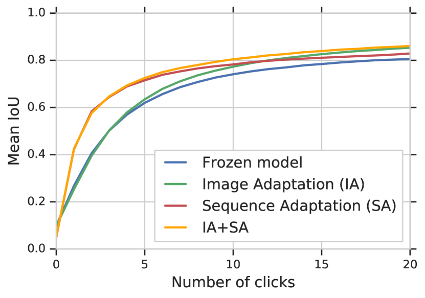
(a) Mean IoU@k for varying $k$ on COCO unseen 6k. Both forms of adaptation significantly improve over a frozen model.

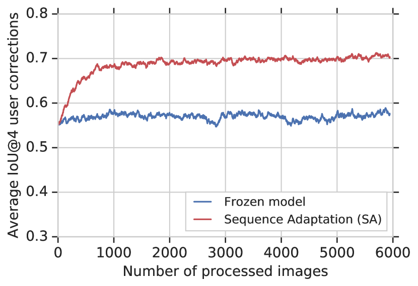
(b) IoU@4 clicks as a function of the number of images processed. SA quickly improves over the model with frozen weights.

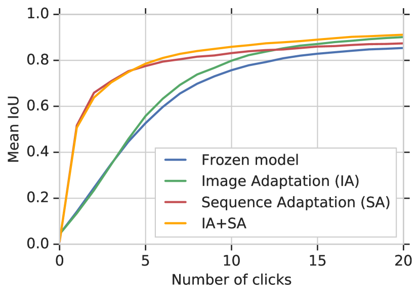
(c) IoU@k for varying $k$ when specializing to donuts. SA offers large gains by learning a class specific appearance model.

Figure 4: Results for adapting to dist. shift (a,b) or a specific class (c).

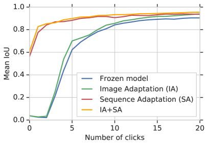
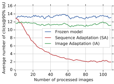
(a) DRIONS-DB dataset.

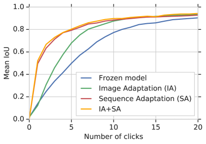
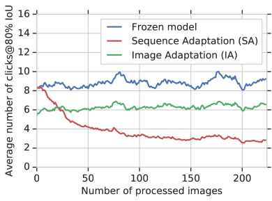
(b) Rooftop Aerial dataset.

Figure 5: Results for domain change. For each dataset, we show the mean IoU at $k$ corrections (left in 5(a), 5(b)) and the number of clicks to reach the target IoU as a function of the number of images processed (right in 5(a), 5(b)). Single image adaptation provides a consistent improvement over the test sequences. Instead, image sequence adaptation adapts its appearance model to the new domain gradually, improving with every image processed (right in 5(a), 5(b)).

Table 2: Class specialization. We test segmenting objects of only one specific class. Our adaptive methods outperforms the frozen model on all tested classes. Naturally, gains are larger for image sequence adaptation, as it can adapt to the class over time.

	clicks @ 85% IoU
	Donut	Bench	Umbrella	Bed
Frozen model [38]	11.6	15.1	13.1	6.8
IA (Ours)	9.2	14.1	11.9	5.5
SA (Ours)	7.1	14.0	11.1	5.5
IA+SA (Ours)	6.5	13.3	10.2	5.0
$\Delta$ over frozen model	44.0%	11.9%	22.1%	26.5%

Table 3: Domain change results. We evaluate our model on 2 datasets that belong to different domains: aerial (Rooftop) and medical (DRIONS-DB). Both types of adaptation (IA and SA) outperform the frozen model.

	DRIONS-DB [14]	Rooftop [53]
Method	clicks@90% IoU	clicks@80% IoU
Frozen model [38]	13.3	8.9
IA (Ours)	11.4	6.3
SA (Ours)	3.6	3.6
IA+SA (Ours)	3.1	3.6
$\Delta$ over frozen model	76.7%	59.6%

4.3 Adapting to domain changes

We test our method’s ability of adapting to domain changes by training on consumer photos (PASCAL VOC12) and evaluating on aerial and medical imagery.

Datasets. We explore two test datasets: (1) Rooftop Aerial [53], a dataset of 65 aerial images with segmented rooftops and (2) DRIONS-DB [14], a dataset of 110 retinal images with a segmentation of the optic disc of the eye fundus. (we use the masks of the first expert). Importantly, the initial model parameters $\boldsymbol{\mathbf{\theta^{*}}}$ were optimized for the PASCAL VOC12 dataset, which consists of consumer photos. Hence, we explore truly large domain changes here.

Results. Both our forms of adaptation significantly improve over the frozen model (Tab. 3, Fig. 5). Single image adaptation can only adapt to a limited extent, as it independently adapts to each object instance, always starting from the same initial model parameters $\boldsymbol{\mathbf{\theta^{*}}}$. Nonetheless, it offers a significant improvement, reducing the number of clicks needed to reach the desired IoU by 14%-29%. Image sequence adaptation (SA) shows extremely strong performance, as its adaptation effects accumulate over the duration of the test sequence. It reduces the needed user input by 60% for the Rooftop Aerial dataset and by over 70% for DRIONS-DB. When combining the two types of adaptation, the reduction increases to 77% for the DRIONS-DB dataset (Tab. 3). Importantly, our method adapts fast: on DRIONS-DB clicks@90% drops quickly and converges to just 2 corrections, as the length of the test sequence increases (Fig. 5(a)). In contrast, the frozen model performs poorly on both datasets. On the Rooftop Aerial dataset, it needs even more clicks than there are points in the ground truth polygons (8.9 vs. 5.1). This shows that even a state-of-the-art model like [38] fails to generalize to truly different domains and highlights the importance of adaptation.

To summarize: We show that our method can bridge large domain changes spanning varied datasets and sequence lengths. With just a single gradient descent step per image, our image sequence adaptation successfully addresses a major shortcoming of neural networks, for the case of interactive segmentation: Their poor generalization to changing distributions [48, 4].

4.4 Comparison to Previous Methods

Table 4: The focus of our work is handling distribution shifts and domain changes between training and testing (Tab. 1, 2 & 3). For completeness, we also compare our method against existing methods on standard datasets, where the distribution mismatch between training and testing is small. At the time of initially releasing our work [32], our method outperformed all previous state-of-the-art models on all datasets. Later, F-BRS [52] (CVPR 2020) achieved even better results.

	VOC12 [20]	GrabCut [49]	Berkeley [40]	DAVIS [43]
	validation			10% of frames
Method	clicks@85%	clicks@90%	clicks@90%	clicks@85%
iFCN w/ GraphCut [56]	6.88	6.04	8.65	-
RIS [35]	5.12	5.00	6.03	-
TSLFN [28]	4.58	3.76	6.49	-
VOS-Wild [10]	5.6	3.8	-	-
ITIS [38]	3.80	5.60	-	-
CAG [39]	3.62	3.58	5.60	-
Latent Diversity [33]	-	4.79	-	5.95
BRS [29]	-	3.60	5.08	5.58
F-BRS [52] (Concurrent Work)	-	2.72	4.57	5.04
IA+SA combined (Ours)	3.18	3.07	4.94	5.16

While the main focus of our work is tackling challenging adaptation scenarios, we also compare our method against state-of-the-art interactive segmentation methods on standard datasets. These datasets are typically similar to PASCAL VOC12, hence have a small distribution mismatch between training and testing.

Datasets. (1) Berkeley, introduced in Sec. 4.1 (2) GrabCut [49], 49 images with segmentation masks. (3) DAVIS16 [43], 50 high-resolution videos out of which we sample 10% of the frames uniformly at random as in [33, 29] (We note that the standard evaluation protocol of DAVIS16 favors adaptive methods, as the same objects appear repeatedly in the test sequence.) and (4) PASCAL VOC12 validation, with 1449 images.

Results. Tab. 4 shows results. Our adaptation method achieves strong results: At the time of initially releasing our work [32], it outperformed all previous state-of-the-art methods on all datasets (it was later overtaken by [52]). It brings improvements even when the previous methods (which have frozen model parameters) already offers strong performance and need less than 4 clicks on average (PASCAL VOC12, GrabCut). The improvement on PASCAL VOC12 further shows that our method helps even when the training and testing distributions match exactly (the frozen model needs 3.44 clicks).

Importantly, we find that our method outperforms [33, 29], even though we use a standard segmentation backbone [17] which predicts at $\frac{1}{4}$ of the input resolution. Instead [33, 29] propose specialized network architectures in order to predict at full image resolution, which is crucial for their good performance [29]. We note that our adaptation method is orthogonal to these architectural optimizations and can be combined with them easily.

4.5 Ablation Study

We ablate the benefit of treating corrections as training examples (on COCO unseen 6k). For this, we selectively remove them from the loss (Eq. (4)). For single image adaptation, this leads to a parameter update that makes the model more confident in its current prediction, but this does not improve the segmentation masks. Instead, training on corrections improves clicks@85% from 13.2 to 10.6. For image sequence adaptation, switching off the corrections corresponds to treating the predicted mask as ground-truth and updating the model with it. This approach implicitly contains corrections in the mask and thus improves  clicks@85% from 13.2 for the frozen model to 11.9. Explicitly using correction offers an additional gain of almost 2 clicks, down to 10. This shows that treating user corrections as training examples is key to our method: They are necessary for single image adaptation and highly beneficial for image sequence adaptation.

4.6 Adaptation speed

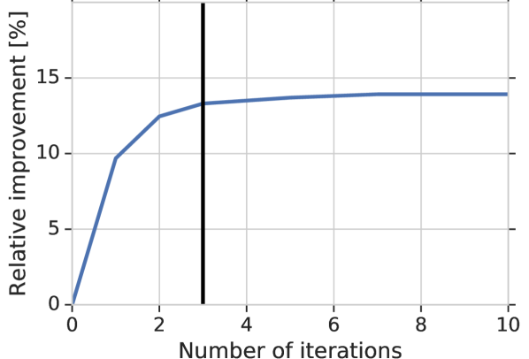
Figure 6: Iterations vs. relative improvement over a frozen model (mean over all datasets).

While our method updates the parameters at test time, it remains fast enough for interactive usage. For the model used throughout our paper a parameter update step takes 0.16 s (Nvidia V100 GPU, mixed-precision training, Berkeley dataset). Image sequence adaptation only needs a single update step, done after an object is segmented (Sec. 3.2.2). Thus, the adaptation overhead is negligible here. For single image adaptation we used 10 update steps, for a total time of 1.6 s. We chose this number of steps based on hyperparameter search (see supp. material). In practice, fewer update steps can be used to increase speed, as they quickly show diminishing returns (Fig. 6). We recommend to use 3 update steps, reducing adaptation time to $0.5$ s, with a negligible effect on the number of corrections required (average difference of less than 1%, over all datasets).
       To increase speed further, the following optimizations are possible: (1) Using a faster backbone, e.g. with a ResNet-50 [27], the time for an update step reduces to 0.06 s; (2) Using faster accelerators such as Google Cloud TPUs; (3) Employing a fixed feature extractor and only updating a light-weight segmentation head [33].

5 Conclusion

We propose to treat user corrections as sparse training examples and introduce a novel method that capitalizes on that idea to update the model parameters on-the-fly at test time. Our extensive evaluation on 8 datasets shows the benefits of our method. When distribution shifts between training and testing are small, our methods offers gains of 9%-30%. When specializing to a specific class, our gains are 12%-44%. For large domain changes, where the imaging modality changes between training and testing, it reduces the required number of user corrections by 60% and 77%.

Acknowledgement. We thank Rodrigo Benenson, Jordi Pont-Tuset, Thomas Mensink and Bastian Leibe for their inputs on this work.

Appendix 0.A Implementation Details

0.A.1 Subsampling for image sequence adaptation

We subsample the corrections in the guidance maps to avoid trivial solutions. If all corrections were used equally in the loss and guidance maps, the model could eventually degrade to predict the corrections given the corrections themselves. Specifically it could degrade to only use the information in the guidance maps as its prediction, without relying on image appearance. We avoid this by subsampling the clicks given to the network as guidance, but using all clicks to compute the adaptation loss (Eq. (4)). This forces the network to rely on appearance for propagating the corrections to the rest of the image, where the loss is sparsely evaluated at the pixel locations which were corrected.

0.A.2 Robustness to image order

Since our image sequence adaptation (SA) and combined adaptation (IA+SA) methods are processing images sequentially, we tested our method’s sensitivity to the image order. We repeated all our experiments 10 times by randomising the image order and computed the variance of the results. We found the variance to be minimal ($\leq 0.01$ standard deviation) verifying that our adaptation methods are not sensitive to the order in which the images are processed. Hence, we only report averages to improve readability.

0.A.3 Adaptation parameters

Our adaptation methods use Adam optimizer [30] with learning rate of $10^{-6}$ and batch size $1$. For single image adaptation we do 10 SGD steps and regularize with $\lambda=1$ and $\gamma=1$. For image sequence adaptation we do 1 SGD step and use $\lambda=0.5$ and $\gamma=2$. For the DRIONS-DB dataset we use a learning rate of $10^{-5}$.

0.A.4 Model details

We use DeeplabV3+ [17] with Xception-65 [18] as our backbone architecture (pre-trained on ImageNet [19] and PASCAL VOC12 [20]). We extend this model with 2 extra channels for the guidance maps and train it for interactive segmentation model using SGD with momentum and an initial learning rate $0.0002$ with polynomial decay. We use a batch size of $2$, and atrous rates $\{12,24,36\}$. We use in input image resolution of $513\times 513$ and an output stride of $8$ for the encoder and $4$ for the decoder, respectively. For generating corrections, we sample at most $5$ foreground and $5$ background corrections for stage one of training (see Sec. 3.3 in the main paper). Corrections are encoded with disks of radius 3.

Appendix 0.B Comparison on the COCO dataset

We have showed that all our adaptation methods are exhibiting substantial improvement compared to the frozen model in many datasets including the COCO dataset. The improvement is especially large on the unseen classes of COCO ($16.8\%$ improvement, Table 1 in the main paper) and on adaptation to a particular unseen class ($44\%$ improvement for the donut class, Table 2 in the main paper), two cases where adaptation is particularly useful.

While we outperform all previous methods on PASCAL VOC12, GrabCut, Berkeley and DAVIS16, some existing works report better clicks@q% than us on COCO. e.g.  [33] reports 7.86 compared to 9.69 for our method. We however note that these results are not directly comparable. 10 instances are sampled per class to form a test set and the selected instances have not been made available by previous works. But how the selection is done is crucial, as segmenting smaller objects is more challenging. If we ignore objects smaller than $80\times 80$ pixels as in [11], for example, our IA+SA improves from 9.9 to 5.4 (4.5 clicks less). Optimizing the architecture to better handle small objects is however not the focus of our work, as our adaptation methods work with any network architecture and can hence be combined with architectural improvements easily.

Appendix 0.C Single image adaptation algorithm

1:function SingleImageAdaptation(input $\boldsymbol{\mathbf{x}}$, labels $\boldsymbol{\mathbf{y}}$, target iou $\mathcal{J}^{t}$, initial parameters $\boldsymbol{\mathbf{\theta}}^{*}$, learning rate $\lambda$, number of steps $k$)

2:   $\boldsymbol{\mathbf{\theta}}\leftarrow\boldsymbol{\mathbf{\theta}}^{*}$ $\triangleright$ Initialize adaptation model

3:   $\boldsymbol{\mathbf{c}}\leftarrow\boldsymbol{\mathbf{-1}}$ $\triangleright$ Start with no corrections

4:   for $i\leftarrow 0..20$ do $\triangleright$ Iterate predicting and correcting

5:     $\boldsymbol{\mathbf{p}}\leftarrow\boldsymbol{\mathbf{f}}(\boldsymbol{\mathbf{x}};\boldsymbol{\mathbf{\theta}})$ $\triangleright$ Predict mask

6:     $\mathcal{J}\leftarrow$ IoU($\boldsymbol{\mathbf{p}},\boldsymbol{\mathbf{y}}$) $\triangleright$ Compute the IOU

7:     if $\mathcal{J}\geq\mathcal{J}^{t}$ then $\triangleright$ Stop if mask has required IOU

8:       return $(\boldsymbol{\mathbf{p}},|\boldsymbol{\mathbf{1}}[\boldsymbol{\mathbf{c}}\neq-1]|,\mathcal{J})$

9:     end if

10:     $\boldsymbol{\mathbf{c}}\leftarrow\boldsymbol{\mathbf{c}}$ $\cup$ GetCorrection($\boldsymbol{\mathbf{x}},\boldsymbol{\mathbf{p}},\boldsymbol{\mathbf{c}}$) $\triangleright$ User input

11:     $\boldsymbol{\mathbf{x}}\leftarrow$ UpdateGuidance($\boldsymbol{\mathbf{x}},\boldsymbol{\mathbf{c}}$)

12:     for $\mathrm{step}\leftarrow 1..k$ do $\triangleright$ Update model parameters

13:       $\boldsymbol{\mathbf{\theta}}\leftarrow\boldsymbol{\mathbf{\theta}}-\lambda\frac{\mathrm{d}}{\mathrm{d}\boldsymbol{\mathbf{\theta}}}\mathcal{L}_{\mathrm{ADAPT}}(\boldsymbol{\mathbf{x}},\boldsymbol{\mathbf{p}},\boldsymbol{\mathbf{c}};\boldsymbol{\mathbf{\theta}})$

14:     end for

15:   end for

16:   return $(\boldsymbol{\mathbf{p}},|\boldsymbol{\mathbf{1}}[\boldsymbol{\mathbf{c}}\neq-1]|,\mathcal{J})$

17:end function

Algorithm 1 Single image adaptation.

Appendix 0.D Number of corrections as proxy for segmentation time

As is common practice [56, 35, 10, 38, 33, 29], we rely on simulated user corrections to evaluate our method. The number of corrections required to reach a certain segmentation quality serves as a proxy for the total time a user requires to segment an object. When less corrections are needed, segmenting an object is generally faster. But the time for making a correction might vary, as it comprises user interaction time (the time it takes for a user to make a correction) and computation time. We now contrast these two factors for our method.

Benenson et al.[11] performed a rigorous user study on interactive segmentation. There, they find that a user spends $\approx 3$ seconds per click correction (not including computation time). For the network used in our work, a single update step takes $0.16$ seconds (Sec. 4.6 in the main paper) and the forward pass takes  0.04 seconds. Thus, single image adaptation requires a computation time of $\approx 0.5s$ with 3 update steps. Image sequence adaptation is even faster as it only requires a single update step, which is done after an object is segmented. Hence, given these timings, user interaction time is the dominating factor for the total segmentation time. Reducing the number of corrections required, as in our work, is therefore an effective way to save user time.

Appendix 0.E Additional Qualitative Results

We show additional results for our two adaptation methods compared to the frozen model in Fig. 7.

\begin{overpic}[trim=0.0pt 0.0pt 0.0pt 28.45274pt,clip,width=433.62pt]{data/both_better/rooftop/99_IMG_0659_inst=0_01_00/5_99_IMG_0659_inst=0_01_00_diffFalse_merged_5.pdf} \put(150.0,220.0){\makebox(0.0,-20.0)[]{\tiny Frozen Model~{}(53.8\%) } } \put(385.0,220.0){\makebox(0.0,-20.0)[]{\tiny IA~{}(91.3\%)}} \put(620.0,220.0){\makebox(0.0,-20.0)[]{\tiny SA~{}(88.3\%)}} \put(855.0,220.0){\makebox(0.0,-20.0)[]{\tiny GT}} \end{overpic}

(a) Rooftop Aerial dataset [53]

\begin{overpic}[trim=0.0pt 0.0pt 0.0pt 28.45274pt,clip,width=433.62pt]{data/coco_unseen/both_better/coco/383_9_id=577451_cat=53_inst=2_01_00/5_383_9_id=577451_cat=53_inst=2_01_00_diffFalse_merged_5.pdf} \put(150.0,400.0){\makebox(0.0,-20.0)[]{\tiny Frozen Model~{}(37.8\%) } } \put(385.0,400.0){\makebox(0.0,-20.0)[]{\tiny IA~{}(91.7\%)}} \put(620.0,400.0){\makebox(0.0,-20.0)[]{\tiny SA~{}(91.2\%)}} \put(860.0,400.0){\makebox(0.0,-20.0)[]{\tiny GT}} \end{overpic}

(b) COCO dataset [36]

\begin{overpic}[trim=0.0pt 0.0pt 0.0pt 28.45274pt,clip,width=433.62pt]{data/grabcut/both_better_select_by_clicksFalse/5_banana3_01_00_Sequence_adaptation.png} \put(150.0,220.0){\makebox(0.0,-20.0)[]{\tiny Frozen Model~{}(81.3\%) } } \put(385.0,220.0){\makebox(0.0,-20.0)[]{\tiny IA~{}(94.6\%)}} \put(620.0,220.0){\makebox(0.0,-20.0)[]{\tiny SA~{}(93.8\%)}} \put(855.0,220.0){\makebox(0.0,-20.0)[]{\tiny GT}} \end{overpic}

(c) GrabCut [49]

Figure 7: Additional results. For each image we show results for our two adaptation methods (IA and SA) and the frozen model for the same number of user corrections (IoU@5 is given in parenthesis). When the frozen model is applied to classes that are unseen during training, it sometimes produces segmentation masks that span multiple objects (7(a) & 7(b)) or do not respect object boundaries (7(c)). Single image adaptation (IA) handles such cases much better, by adapting the model parameters to that specific object and its background. This allows it to correctly segment objects even when the foreground and background have similar appearance (7(b)). Image sequence adaptation (SA) optimizes the model parameters for the test sequence. This allows it to produce good masks from very few clicks, and additional clicks are only required close to the object to refine the exact boundary (7(a) & 7(c)).

References

- [1] Acuna, D., Ling, H., Kar, A., Fidler, S.: Efficient Interactive Annotation of Segmentation Datasets with Polygon-RNN++. In: CVPR (2018)
- [2] Adobe: Select a subject with just one click. https://helpx.adobe.com/photoshop/how-to/select-subject-one-click.html (2018)
- [3] Agustsson, E., Uijlings, J.R., Ferrari, V.: Interactive full image segmentation by considering all regions jointly. In: CVPR (2019)
- [4] Alcorn, M.A., Li, Q., Gong, Z., Wang, C., Mai, L., Ku, W.S., Nguyen, A.: Strike (with) a pose: Neural networks are easily fooled by strange poses of familiar objects. In: CVPR (2019)
- [5] Aljundi, R., Babiloni, F., Elhoseiny, M., Rohrbach, M., Tuytelaars, T.: Memory aware synapses: Learning what (not) to forget. In: ECCV (2018)
- [6] Aljundi, R., Kelchtermans, K., Tuytelaars, T.: Task-free continual learning. In: CVPR (2019)
- [7] Bai, X., Sapiro, G.: Geodesic matting: A framework for fast interactive image and video segmentation and matting. IJCV (2009)
- [8] Bearman, A., Russakovsky, O., Ferrari, V., Fei-Fei, L.: What’s the point: Semantic segmentation with point supervision. In: ECCV (2016)
- [9] Belouadah, E., Popescu, A.: Il2m: Class incremental learning with dual memory. In: ICCV (2019)
- [10] Benard, A., Gygli, M.: Interactive video object segmentation in the wild. arXiv (2017)
- [11] Benenson, R., Popov, S., Ferrari, V.: Large-scale interactive object segmentation with human annotators. In: CVPR (2019)
- [12] Boykov, Y., Jolly, M.P.: Interactive graph cuts for optimal boundary and region segmentation of objects in N-D images. In: ICCV (2001)
- [13] Caelles, S., Maninis, K.K., Pont-Tuset, J., Leal-Taixé, L., Cremers, D., Van Gool, L.: One-shot video object segmentation. In: CVPR (2017)
- [14] Carmona, E.J., Rincón, M., García-Feijoó, J., Martínez-de-la Casa, J.M.: Identification of the optic nerve head with genetic algorithms. Artificial Intelligence in Medicine (2008)
- [15] Castrejón, L., Kundu, K., Urtasun, R., Fidler, S.: Annotating object instances with a Polygon-RNN. In: CVPR (2017)
- [16] Chen, D.J., Chien, J.T., Chen, H.T., Chang, L.W.: Tap and shoot segmentation. In: AAAI (2018)
- [17] Chen, L.C., Zhu, Y., Papandreou, G., Schroff, F., Adam, H.: Encoder-decoder with atrous separable convolution for semantic image segmentation. In: ECCV (2018)
- [18] Chollet, F.: Xception: Deep learning with depthwise separable convolutions. In: CVPR (2017)
- [19] Deng, J., Dong, W., Socher, R., Li, L.J., Li, K., Fei-fei, L.: ImageNet: A large-scale hierarchical image database. In: CVPR (2009)
- [20] Everingham, M., Van Gool, L., Williams, C.K.I., Winn, J., Zisserman, A.: The PASCAL Visual Object Classes Challenge 2012 (VOC2012) Results. http://www.pascal-network.org/challenges/VOC/voc2012/workshop/index.html (2012)
- [21] Farquhar, S., Gal, Y.: Towards robust evaluations of continual learning. arXiv (2018)
- [22] Finn, C., Abbeel, P., Levine, S.: Model-agnostic meta-learning for fast adaptation of deep networks. In: ICML (2017)
- [23] Gatys, L.A., Ecker, A.S., Bethge, M.: Image style transfer using convolutional neural networks. In: CVPR (2016)
- [24] Gulshan, V., Rother, C., Criminisi, A., Blake, A., Zisserman, A.: Geodesic star convexity for interactive image segmentation. In: CVPR (2010)
- [25] Gygli, M., Norouzi, M., Angelova, A.: Deep value networks learn to evaluate and iteratively refine structured outputs. In: ICML (2017)
- [26] Hariharan, B., Arbeláez, P., Bourdev, L., Maji, S., Malik, J.: Semantic contours from inverse detectors. In: ICCV (2011)
- [27] He, K., Zhang, X., Ren, S., Sun, J.: Deep residual learning for image recognition. arXiv preprint arXiv:1512.03385 (2015)
- [28] Hu, Y., Soltoggio, A., Lock, R., Carter, S.: A fully convolutional two-stream fusion network for interactive image segmentation. Neural Networks (2019)
- [29] Jang, W.D., Kim, C.S.: Interactive image segmentation via backpropagating refinement scheme. In: CVPR (2019)
- [30] Kingma, D.P., Ba, J.L.: Adam: A method for stochastic optimization. In: ICLR (2015)
- [31] Kirkpatrick, J., Pascanu, R., Rabinowitz, N., Veness, J., Desjardins, G., Rusu, A.A., Milan, K., Quan, J., Ramalho, T., Grabska-Barwinska, A., et al.: Overcoming catastrophic forgetting in neural networks. Proc. Nat. Acad. Sci. USA (2017)
- [32] Kontogianni, T., Gygli, M., Uijlings, J., Ferrari, V.: Continuous adaptation for interactive object segmentation by learning from corrections. arXiv preprint arXiv:1911.12709v1 (2019)
- [33] Li, Z., Chen, Q., Koltun, V.: Interactive image segmentation with latent diversity. In: CVPR (2018)
- [34] Li, Z., Hoiem, D.: Learning without forgetting. IEEE Trans. on PAMI (2017)
- [35] Liew, J., Wei, Y., Xiong, W., Ong, S.H., Feng, J.: Regional interactive image segmentation networks. In: ICCV (2017)
- [36] Lin, T.Y., Maire, M., Belongie, S., Hays, J., Perona, P., Ramanan, D., Dollár, P., Zitnick, C.: Microsoft COCO: Common objects in context. In: ECCV (2014)
- [37] Ling, H., Gao, J., Kar, A., Chen, W., Fidler, S.: Fast interactive object annotation with Curve-GCN. In: CVPR (2019)
- [38] Mahadevan, S., Voigtlaender, P., Leibe, B.: Iteratively trained interactive segmentation. In: BMVC (2018)
- [39] Majumder, S., Yao, A.: Content-aware multi-level guidance for interactive instance segmentation. In: CVPR (2019)
- [40] McGuinness, K., O’connor, N.E.: A comparative evaluation of interactive segmentation algorithms. Pattern Recognition (2010)
- [41] Michieli, U., Zanuttigh, P.: Incremental learning techniques for semantic segmentation. In: ICCV Workshop (2019)
- [42] Papadopoulos, D.P., Uijlings, J.R.R., Keller, F., Ferrari, V.: We don’t need no bounding-boxes: Training object class detectors using only human verification. In: CVPR (2016)
- [43] Perazzi, F., Pont-Tuset, J., McWilliams, B., Van Gool, L., Gross, M., Sorkine-Hornung, A.: A benchmark dataset and evaluation methodology for video object segmentation. In: CVPR (2016)
- [44] Price, B.L., Morse, B., Cohen, S.: Geodesic graph cut for interactive image segmentation. In: CVPR (2010)
- [45] Qi, S., Zhu, Y., Huang, S., Jiang, C., Zhu, S.C.: Human-centric indoor scene synthesis using stochastic grammar. In: CVPR (2018)
- [46] Ravi, S., Larochelle, H.: Optimization as a model for few-shot learning. In: ICLR (2016)
- [47] Rebuffi, S., Kolesnikov, A., Sperl, G., Lampert, C.: icarl: Incremental classifier and representation learning. In: CVPR (2017)
- [48] Recht, B., Roelofs, R., Schmidt, L., Shankar, V.: Do CIFAR-10 classifiers generalize to CIFAR-10? arXiv (2018)
- [49] Rother, C., Kolmogorov, V., Blake, A.: GrabCut - Interactive Foreground Extraction using Iterated Graph Cut. SIGGRAPH 23 (2004)
- [50] Shmelkov, K., Schmid, C., Alahari, K.: Incremental learning of object detectors without catastrophic forgetting. In: ICCV (2017)
- [51] Snell, J., Swersky, K., Zemel, R.: Prototypical networks for few-shot learning. In: NeurIPS (2017)
- [52] Sofiiuk, K., Petrov, I., Barinova, O., Konushin, A.: F-BRS: Rethinking Backpropagating Refinement for Interactive Segmentation. In: CVPR (2020)
- [53] Sun, X., Christoudias, C.M., Fua, P.: Free-shape polygonal object localization. In: ECCV (2014)
- [54] Sun, Y., Wang, X., Liu, Z., Miller, J., Efros, A.A., Hardt, M.: Test-time training for out-of-distribution generalization. arXiv (2019)
- [55] Voigtlaender, P., Leibe, B.: Online adaptation of convolutional neural networks for video object segmentation. In: BMVC (2017)
- [56] Xu, N., Price, B., Cohen, S., Yang, J., Huang, T.: Deep interactive object selection. In: CVPR (2016)
- [57] Xu, N., Yang, L., Fan, Y., Yue, D., Liang, Y., Yang, J., Huang, T.: YouTube-VOS: A Large-Scale Video Object Segmentation Benchmark. arXiv (2018)
- [58] Zenke, F., Poole, B., Ganguli, S.: Continual learning through synaptic intelligence. In: ICML (2017)
- [59] Zhou, B., Zhao, H., Puig, X., Fidler, S., Barriuso, A., Torralba, A.: Scene parsing through ADE20K dataset. In: CVPR (2017)
- [60] Zhou, B., Zhao, H., Puig, X., Fidler, S., Barriuso, A., Torralba, A.: Semantic understanding of scenes through the ADE20K dataset. IJCV (2018)
- [61] Zhou, Z., Shin, J., Zhang, L., Gurudu, S., Gotway, M., Liang, J.: Fine-tuning convolutional neural networks for biomedical image analysis: actively and incrementally. In: CVPR (2017)