Spin structure of hadrons and minimum energy of bound systems

Abstract

The spin of a composite particle, like a nucleus or a hadron, is generated by the composition of angular moments (consisting of spins and orbital angular moments) of the constituents. The composition of two angular moments is done by the standard way with the use of Clebsch-Gordan coefficients. However, if there are more than two constituents, the composition must be done in a hierarchical way, which admits more ways leading to the same resulting spin state $\left|J,J_{z}\right\rangle$. Different composition patterns can generate states with the same spin quantum numbers, but which may vary in the contributions of different kinds of the constituents. We will discuss which composition patterns could be preferred in the hadrons from the viewpoint of minimal energy of the bound system. In this context, particular attention is paid to the role of gluons or quark orbital angular momentum in the proton spin.

I Introduction

Spin structure of hadrons that consist of quarks and gluons generating bond among them is a difficult nonperturbative QCD problem. The complexity of this task can be illustrated by a long history of the proton spin puzzle that began with the EMC experiment emc . Let’s remind the main facts.

Before the well-known surprising result of the EMC experiment, it was expected that the proton spin is simply defined by the sum of the spins of quarks inside the proton. This expectation was disproved by measuring the structure function $g_{1}(x)$, whose integral

$$\Gamma_{1}=\int g_{1}(x)dx$$ (1)

allows us to evaluate the total contribution of the quark spins. It has been shown that the spins of quarks represent only a small part of the proton spin. This result was confirmed by further experiments that followed. At present, the precise measurement of the Compass experiment compsig implies the spins of quarks represent only about $1/3$ of the proton spin. The small quark contribution $\Delta\Sigma$ raised the question of how the proton spin is actually generated? It is currently assumed that two additional contributions may be relevant:

i) The total angular momentum of gluons can make a significant contribution. If gluons can make up about half of the proton energy (mass), why would they not significantly contribute to the spin? And if so, how much?

ii) Quark orbital angular momentum (OAM) can also significantly contribute to the proton spin. The intrinsic motion of quarks localized inside the proton can generate OAM, but how large?

The present study aims to discuss the task of AMs composition in the many-body quantum mechanical systems and the implications related to these questions. The main goal of this note is to show the argument why the gluon contribution to the spin of most stable hadrons should be rather small (Sec.2). We also remind our former arguments in favor of the important role of quark OAM (Sec.3).  A short discussion is presented in Sec.4.

II Interplay of the AMs inside the hadron

Hadrons are the eigenstates $\Psi=|J,J_{z}\rangle$ of two commuting spin operators $\hat{J}^{2}=\hat{J}_{x}^{2}+\hat{J}_{y}^{2}+\hat{J}_{z}^{2}$ and $\hat{J}_{z}$ with the eigenvalues

$$\hat{J}^{2}\Psi=J\left(J+1\right)\hbar^{2}\Psi,\quad\hat{J}_{z}\Psi=J_{z}\hbar\Psi;\quad-J\leq J_{z}\leq J,$$ (2)

where $J$ and $J_{z}$ are integers for mesons and half-integers for baryons. The operators $\hat{J}_{x},\hat{J}_{y}$ and $\hat{J}_{z}$ represent the spin projections on three axes $x,y,z$, AM is a three-dimensional quantity. The hadrons are composite particles consisting of quarks and gluons, so their spin (total AM) is generated by the AM of their constituents, quarks and gluons. The AM operators consist of the corresponding spin and OAM:

$$\hat{\jmath}=\hat{s}+\hat{l}.$$ (3)

The hadron rest frame is natural (initial) reference frame for their composition.

II.1 Composition of the AMs

In quantum mechanics the binary AM composition is defined as

$$\left|(j_{1},j_{2})J,J_{z}\right\rangle =\sum_{j_{z1}=-j_{1}}^{j_{1}}\sum_{j_{z2}=-j_{2}}^{j_{2}}\left\langle j_{1},j_{z1},j_{2},j_{z2}\left|J,J_{z}\right.\right\rangle\left|j_{1},j_{z1}\right\rangle\left|j_{2},j_{z2}\right\rangle;$$ (4)

$$j_{z1}+j_{z2} =J_{z},\qquad\qquad\qquad\left|j_{1}-j_{2}\right|\leq J\leq j_{1}+j_{2},$$ (5)

where $\left\langle j_{1},j_{z1},j_{2},j_{z2}\left|J,J_{z}\right.\right\rangle$ are Clebsch-Gordan coefficients, which are non-zero only if the conditions (5) are satisfied. The symbols $j_{i},j_{zi}$ are related to the total AM of the constituents (3), $J,J_{z}$ are the spin numbers of the hadron. The relation represents rule for AM composition of $j_{1},j_{2}$ resulting in $J,$ symbolically $\left(j_{1}\oplus j_{2}\right)_{J}$. If there are more then two AMs to compose, one must repeat the binary composition to obtain the many-particle eigenstates of resulting $J,J_{z}$

$$\left|(j_{1},j_{2},...j_{n})_{c}J,J_{z}\right\rangle=\sum_{j_{z1}=-j_{1}}^{j_{1}}\sum_{j_{z2}=-j_{2}}^{j_{2}}...\sum_{j_{zn}=-j_{n}}^{j_{n}}c_{j}\left|j_{1},j_{z1}\right\rangle\left|j_{2},j_{z2}\right\rangle...\left|j_{n},j_{zn}\right\rangle,$$ (6)

where the coefficients $c_{j}$ consist of the Clebsch-Gordan coefficients

$$c_{j}=\left\langle j_{1},j_{z1},j_{2},j_{z2}\left|J_{3},J_{3z}\right.\right\rangle\left\langle J_{3},J_{z3},j_{3},j_{z3}\left|J_{4},J_{z4}\right.\right\rangle...\left\langle J_{n},J_{zn},j_{n},j_{zn}\left|J,J_{z}\right.\right\rangle.$$ (7)

However the set $j_{1},j_{2},..j_{n}$ does not define the resulting state $J$ unambiguously, this state depends also on the intermediate values $J_{1},J_{2}...$, and the order of composition. The subscript $c$ in l.h.s. of (6) denotes a definite pattern of composition. In Fig. 1 we show symbolic examples of a few composition patterns for two quarks and one or two gluons.

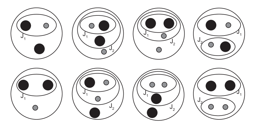
Figure 1: Examples of AM composition patterns for meson. Greater black spots represent quarks, smaller grey ones are gluons.

Similar examples for three quarks and one gluon follow in Fig. 2.

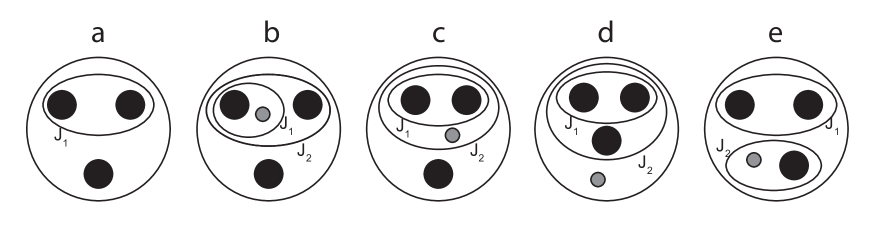
Figure 2: Examples of AM composition patterns for baryon. The spots are quarks and gluons, like in the previous picture.

The patterns in the figures can be labeled as

$$c=(((j_{1}\oplus j_{2})_{J_{1}}\oplus j_{3})_{J_{2}}\oplus k_{1})_{J}$$ (8)

for Fig. 2d and similarly for others. The symbol (8) represents three consecutive steps of composition (4) giving the states

$$\left|(j_{1},j_{2})J_{1},J_{1z}\right\rangle,\qquad\left|(J_{1},j_{3})J_{2},J_{2z}\right\rangle,\qquad\left|(J_{2},k)J,J_{z}\right\rangle,$$ (9)

where $J_{i}$ represent intermediate AMs:

$$j_{1}\oplus j_{2}=J_{1},\qquad J_{1}\oplus j_{3}=J_{2},\qquad J_{2}\oplus k=J.$$ (10)

A priory various patterns for a fixed $J$ can be allowed, but their number increases with the number of the constituents in the composition very fast. The real state can be some superposition of the Fock states defined by these patterns. At the same time in the real scenario of interacting particles, one can expect their probabilities will vary, but which patterns will be preferred? And how can the states with the same resulting spin differ?

II.2 Bound systems

We work with the many particle stationary states that are controlled by the unperturbative QCD, which does not give much hope for a simple solution. On the other hand, even without knowledge of the solution of complicated equations it is known that stable or quasi-stable systems are always associated with some (rest frame) energy minimum. So we will discuss which type of patterns can prefer lower energy minimum.

Let us recall the role of AM in a few well-known examples of bound, stable or quasi-stable systems:

a) In atoms higher OAM of electrons correlate with higher energy levels. At the same time, the electrons in noble gases having fully occupied energy levels with total AM equal zero are the most stable atoms. Noble gases have the largest ionization potential for each period.

b) Even-even nuclei have always total spin $J=0$ and are known to be more stable. Some good examples are ${}_{2}^{4}$He, ${}_{6}^{12}$C and ${}_{8}^{16}$O.

c) The excited states of mesons and nucleons are associated with higher masses (energy) together with higher spins. For example $\rho(770)^{0\pm}$ mesons are excited states of pions, resonances $\Delta(1232)^{0+}$ are excited neutron and proton. The empirical almost linear dependencies $M^{2}$ on $J$ for the families of meson and baryon resonances regge are known as the Regge trajectories.

The systems b),c) are controlled by the QCD. The examples suggest the correlation:

$$energy\ (mass)\sim total\ AM\ (spin),\quad minimum\ energy\sim minimum\ AM$$

Obviously:

$\bullet$ Minimum energy is a manifestation of the bond

$\bullet$ Bond generates a tendency to minimum AM:

Presence of gluons (color field) mediating bond among quarks generates lower energy, which generates minimum AM of the corresponding state (or segment). The minimum energy of gluons is not influenced by the Pauli principle. So, we shall try to work with the rule:

Presence of the gluons is preferred in the segments of $J=0$:

$$(...(...\oplus k)...)_{J=0},$$ (11)

where $k$ is the gluon AM. It is important that any composition pattern for particles of arbitrary AMs $j_{1},j_{2},...j_{n\text{ }}$ generating the state $J=0$, gives also the condition for all $j_{zi}:$

$$\left\langle j_{z1}\right\rangle=\left\langle j_{z2}\right\rangle=....=\left\langle j_{zn}\right\rangle=0.$$ (12)

This rule together with the relation

$$\left\langle j_{z1}\right\rangle+\left\langle j_{z2}\right\rangle+....+\left\langle j_{zn}\right\rangle=J_{z},$$ (13)

are proved in Appendix. We will discuss consequences of (11) for hadrons with minimum spin: $J=0$ (mesons) and $J=1/2$ (baryons). Obviously, obtained condition (12) is stronger than

$$\left\langle j_{z1}\right\rangle+\left\langle j_{z2}\right\rangle+....+\left\langle j_{zn}\right\rangle=0.$$ (14)

To simplify the discussion, we do not strictly distinguish quarks, antiquarks and their flavors, only their AMs are important.

II.3 Mesons of spin $J=0$

We assume arbitrary patterns involving $2n$ quarks and any number of gluons, which generate the state $J=J_{z}=0$. Examples of such systems are mesons $\pi,\eta,K,D,$ etc. The rule of preference (11) is satisfied automatically, then the rule (12) means that

$$\left\langle j_{z}^{a}\right\rangle=0,$$ (15)

where $a$ denotes constituents: quarks and gluons. It means that average AMs of gluons and quarks of any flavor are zero in the scalar or pseudoscalar mesons.

II.4 Baryons of spin $J=1/2$

Now we assume arbitrary patterns with $3+2n$ quarks and any number of gluons, which generate states of minimum spin content, $J=J_{z}=1/2$. The examples in Fig. 2 are completed by Tab. 1.

Table 1: Examples of composition patterns

	Composition pattern	$\left\langle j_{z1}\right\rangle,\left\langle j_{z2}\right\rangle,\left\langle j_{z3}\right\rangle,\left\langle k_{z}\right\rangle$
a	$\left(\left(j_{1}\oplus j_{2}\right)_{0}\oplus j_{3}\right)_{1/2}$	$\ \ \ 0,\ \ \ \ \ 0,\ \ \ \ \frac{1}{2},\ \ \ 0$
b1	$\left(\left(\left(j_{1}\oplus k\right)_{1/2}\oplus j_{2}\right)_{0}\oplus j_{3}\right)_{1/2}$	$\ \ \ 0,\ \ \ \ \ 0,\ \ \ \ \frac{1}{2},\ \ \ 0$
b2	$\left(\left(\left(j_{1}\oplus k\right)_{1/2}\oplus j_{2}\right)_{1}\oplus j_{3}\right)_{1/2}$	$\frac{-1}{9},\ \ \ \ \frac{1}{3},\ \ \frac{-1}{6},\ \ \frac{4}{9}$
c	$\left(\left(\left(j_{1}\oplus j_{2}\right)_{1}\oplus k\right)_{0}\oplus j_{3}\right)_{1/2}$	$\ \ \ 0,\ \ \ \ \ 0,\ \ \ \ \frac{1}{2},\ \ 0$
d1	$\left(\left(\left(j_{1}\oplus j_{2}\right)_{0}\oplus j_{3}\right)_{1/2}\oplus k\right)_{1/2}$	$\ \ \ 0,\ \ \ \ \ 0,\ \ \frac{-1}{6},\ \frac{2}{3}$
d2	$\left(\left(\left(j_{1}\oplus j_{2}\right)_{1}\oplus j_{3}\right)_{1/2}\oplus k\right)_{1/2}$	$\frac{-1}{9},\ \ \frac{-1}{9},\ \ \ \frac{1}{18},\ \frac{2}{3}$
e1	$\left(\left(j_{1}\oplus j_{2}\right)_{0}\oplus\left(j_{3}\oplus k\right)_{1/2}\right)_{1/2}$	$\ \ \ 0,\ \ \ \ \ 0,\ \ \frac{-1}{6},\ \frac{2}{3}$
e2	$\left(\left(j_{1}\oplus j_{2}\right)_{1}\oplus\left(j_{3}\oplus k\right)_{1/2}\right)_{1/2}$	$\ \ \frac{1}{3},\ \ \ \frac{1}{3},\ \ \frac{1}{18},\ \frac{-2}{9}$

All patterns in figure generate composite fermion of the same spin, but in general the states are different. The patterns differ in the right column of the table, where the quark and gluon contributions vary, but satisfy

$$\left\langle j_{z1}\right\rangle+\left\langle j_{z2}\right\rangle+\left\langle j_{z3}\right\rangle+\left\langle k_{z}\right\rangle=\frac{1}{2},$$ (16)

which is a special case of (13).

a) A toy model: scenario $3q+gluons$

Obviously the preferred segments (11) are present only in the patterns b₁ and c in table and in corresponding panels of Fig. 2. Here the gluon is shared by two quarks within an intermediate state with $J=0$. Corresponding baryon state is generated by a superposition of both patterns with the permutations of the three quarks. In a more general version one can consider any number of gluons shared by two the quarks within the state $J=0$. For example, there can be some correspondence between this scenario and the known quark-diquark model q2q . The rule of preference (11) suppresses the contribution of gluon AM.

b) General scenario $3q+nq\bar{q}+gluons$

The numbers of sea quarks and gluons are not fixed and baryon state is represented by a corresponding superposition of the Fock states $J=J_{z}=1/2,$ which are constrained by the rule of preference (11). Preferred segments in patterns b₁ and c in the table are just simple examples. In general scenario, preferred segments can create more complex quark-gluon states of spin $J=0$, for which the condition (12) is satisfied. It follows, that average quark and gluon AM contributions are zero in these segments. Since we assume the gluons sit only in preferred segments (11), the total gluon AM contribution must be suppressed in the resulting Fock states. We talk about the total gluon AM and avoid the controversies in its splitting to the spin and orbital part, as analyzed thoroughly in Leader:2013jra .

II.5 Connection with QCD

In general, the structure of hadrons results from QCD, which is represented by a complex system of differential equations. A prerequisite for the solution of the system is the specification of boundary conditions defining the hadron. In addition to the composition of the bound system (a type of meson, baryon or nucleus, including its spin) a condition of minimum energy in the hadron rest frame is required. As we have suggested, minimum energy can be correlated with the particular AM composition patterns. In this sense, our discussion is related to the QCD boundary conditions.

III Reason for quark OAM

We have studied the role of the quark OAM in the covariant quark-parton model Zavada:2007ww ; Zavada:2013ola ; Zavada:2015gaa ; Zavada:2002uz ; Zavada:2001bq , the essence is as follows. For Dirac particle, it is known that in relativistic case the spin $\left(s,s_{z}\right)$ and OAM $\left(l,l_{z}\right)$ are not decoupled (separately conserved), but only quantum numbers $j,j_{z}$ corresponding to the total angular momentum (AM) are conserved ($j,j_{z}$ are the good quantum numbers). However, one can always calculate the mean values $\left\langle s_{z}\right\rangle$ and $\left\langle l_{z}\right\rangle,$ and it holds

$$j_{z}=\left\langle s_{z}\right\rangle+\left\langle l_{z}\right\rangle.$$ (17)

We have studied this issue in the representation of spinor spherical harmonics, which allowed us to explore this relativistic spin-orbit interplay more explicitly. From general relations

$$\left\langle s_{z}\right\rangle_{j,j_{z}}=\frac{1+\left(2j+1\right)\mu}{4j\left(j+1\right)}j_{z},\qquad\left\langle l_{z}\right\rangle_{j,j_{z}}=\left(1-\frac{1+\left(2j+1\right)\mu}{4j\left(j+1\right)}\right)j_{z}$$ (18)

we obtained for particle of spin $1/2$ in the state $j=j_{z}=1/2$

$$\left\langle s_{z}\right\rangle=\frac{1+2\mu}{6},\qquad\left\langle l_{z}\right\rangle=\frac{1-\mu}{3};\qquad\mu=\frac{m}{\epsilon},$$ (19)

where $m$ and  $\epsilon$  are mass and energy of the particle. So, for non-relativistic $\left(\mu\rightarrow 1\right)$ case we have

$$\left\langle s_{z}\right\rangle=j_{z}=1/2,\quad\left\langle l_{z}\right\rangle=0;$$ (20)

and for relativistic one $\left(\mu\rightarrow 0\right)$

$$\left\langle s_{z}\right\rangle=1/6,\quad\left\langle l_{z}\right\rangle=1/3,\quad\left\langle s_{z}\right\rangle+\left\langle l_{z}\right\rangle=j_{z}=1/2.$$ (21)

The last relation represents a kinematical effect in relativistic quantum mechanics. This effect is exactly reproduced in the covariant quark-parton model, where the effective value of $\mu$ is a free parameter. Other representations of the relativistic suppression of the quark spin are discussed in the papers Zhang:2012sta ; Ma:2001ui ; Qing:1998at ; Liang:1996je ; Ma:1992sj ; Ma:1991xq . The last relation, corresponding to $\mu_{eff}\rightarrow 0,$ represents the scenario of massless quarks. The quark spin contribution to the proton spin is $\Sigma\approx 1/3$ and the missing part is balanced by the quark OAM. It means a very good agreement with the data compsig even without a gluon contribution. At the same time, the same experiment compglu suggests gluon contribution rather small. In general scenario $\mu_{eff}>0$, then (19) implies that contribution of the quark OAM should be less, so some gluon contribution is needed to explain the data on $\Sigma$. Such a prediction could be consistent with the data star .

IV Discussion and conclusion

In our approach, the following conditions are necessary:

1) Also in the covariant parton model, we assume that in deep inelastic scattering the quarks can be considered quasi-free. If this assumption is met in the infinite momentum frame, it is also met in other reference systems - including the nucleon rest frame Zavada:2013ola .

2) Rest frame of the composite system (nucleon) with 3D rotation invariance is necessary condition for quantum mechanical composition of spins and orbital moments of the constituents, with the use of Clebsch-Gordan coefficients. At the same time, for bound systems, the rest frame is necessary for the expression of the minimum-energy condition.

The second condition allows us to use the representation of spinor spherical harmonics, which implies the spin-orbit interplay is controlled by the ratio $m/\epsilon$. Obviously, the 3D rotational invariance of the rest frame is not fulfilled for the current light-cone formalism. That is why a similar spin-orbit constraint is missing. In the covariant model, the assumptions formulated in the rest frame generate the shape and properties of (invariant) structure functions.

In this report we have studied the AM composition in many (quasi-free) particle systems. We focused on hadrons and in particular on the proton. We suggested argument, why the AM contribution of gluons to the proton spin should be rather small. At the same time, we have discussed the important role of the quark OAM following from kinematical effect of relativistic quantum mechanics, which is simply reproduced in the covariant quark-parton model, but not in the light-cone formalism.

Appendix A Proof of relations (16), (12)

Lemma 1

Any composition pattern for particles of arbitrary integer or half-integer $j_{1},j_{2},...j_{n\text{ }}$ that generates state $J=0$, implies the condition for all $j_{zi}:$

$$\left\langle j_{z1}\right\rangle=\left\langle j_{z2}\right\rangle=....=\left\langle j_{zn}\right\rangle=0.$$ (22)

Proof:  For the state

$$\left|(j_{1},j_{2},...j_{n})_{c}J,J_{z}\right\rangle=\sum_{j_{z1}=-j_{1}}^{j_{1}}\sum_{j_{z2}=-j_{2}}^{j_{2}}...\sum_{j_{zn}=-j_{n}}^{j_{n}}c_{j}\left|j_{1},j_{z1}\right\rangle\left|j_{2},j_{z2}\right\rangle...\left|j_{n},j_{zn}\right\rangle,$$ (23)

where the coefficients $c_{j}$ consist of the Clebsch-Gordan coefficients

$$c_{j}=\left\langle j_{1},j_{z1},j_{2},j_{z2}\left|J_{3},J_{3z}\right.\right\rangle\left\langle J_{3},J_{z3},j_{3},j_{z3}\left|J_{4},J_{z4}\right.\right\rangle...\left\langle J_{n},J_{zn},j_{n},j_{zn}\left|J,J_{z}\right.\right\rangle,$$ (24)

we calculate average $j_{z1}$:

$$\left\langle j_{z1}\right\rangle=\sum_{j_{z1}=-j_{1}}^{j_{1}}j_{z1}\sum_{j_{z2}=-j_{2}}^{j_{2}}...\sum_{j_{zn}=-j_{n}}^{j_{n}}c_{j}c_{j}^{\ast}=\sum_{j_{z1}=-j_{1}}^{j_{1}}j_{z1}w\left(j_{z1}\right).$$ (25)

The Clebch-Gordan coefficients are real and it holds:

$$\left\langle j_{k},j_{zk},j_{l},j_{zl}\left|J_{i},J_{iz}\right.\right\rangle=\left(-1\right)^{J_{i}-j_{k}-j_{l}}\left\langle j_{k},-j_{zk},j_{l},-j_{zl}\left|J_{i},-J_{iz}\right.\right\rangle.$$ (26)

For $J=J_{z}=0$ the term

$$w\left(j_{z1}\right)=\sum_{j_{z2}=-j_{2}}^{j_{2}}...\sum_{j_{zn}=-j_{n}}^{j_{n}}c_{j}c_{j}^{\ast}>0$$ (27)

is in the sum (25) always accompanied by the term $w\left(-j_{z1}\right)$ and

$$w\left(j_{z1}\right)=w\left(-j_{z1}\right),$$ (28)

which implies $\left\langle j_{z1}\right\rangle=0$. Similarly for others in (22).

ii) Relation (13)

Eq. (6) implies

$$\left\langle j_{z1}\right\rangle+\left\langle j_{z2}\right\rangle+...\left\langle j_{zn}\right\rangle =\left\langle j_{z1}+j_{z2}+...j_{zn}\right\rangle$$

$$=\sum_{j_{z1}=-j_{1}}^{j_{1}}\sum_{j_{z2}=-j_{2}}^{j_{2}}...\sum_{j_{zn}=-j_{n}}^{j_{n}}c_{j}c_{j}^{\ast}\left(j_{z1}+j_{z2}+...j_{zn}\right)$$

$$=\sum_{j_{z1}=-j_{1}}^{j_{1}}\sum_{j_{z2}=-j_{2}}^{j_{2}}...\sum_{j_{zn}=-j_{n}}^{j_{n}}c_{j}c_{j}^{\ast}J_{z}=J_{z}.$$ (29)

Relation (16) is a special case of this equation.

References

• (1) J. Ashman et al. [EMC Collaboration], Nucl. Phys. B 238, 1 (1990); Phys. Lett. B 206, 364 (1988).
• (2) V. Y. .Alexakhin et al. [COMPASS Collaboration], Phys. Lett. B 647, 8 (2007).
• (3) C. Adolph et al. [COMPASS Collaboration], Phys. Lett. B 718, 922 (2013).
• (4) L. Adamczyk et al. [STAR Collaboration], Phys. Rev. Lett. 115, no. 9, 092002 (2015).
• (5) Alfred Tang and John W. Norbury, Phys. Rev. D 62, 016006(2000).
• (6) D. B. Lichtenberg and L. J. Tassie, Phys. Rev. 155, 1601(1967).
• (7) E.Β Leader and C.Β LorcΓ©, Phys.Β Rept.Β 541, no. 3, 163 (2014).
• (8) P.Β Zavada, Phys.Β Lett.Β B 751, 525 (2015).
• (9) P.Β Zavada, Phys.Β Rev.Β D 89, no. 1, 014012 (2014).
• (10) P.Β Zavada, Eur.Β Phys.Β J.Β C 52, 121 (2007).
• (11) P.Β Zavada, Phys.Β Rev.Β D 67, 014019 (2003).
• (12) P.Β Zavada, Phys.Β Rev.Β D 65, 054040 (2002).
• (13) X.Β Zhang and B.Β Q.Β Ma, Phys.Β Rev.Β D 85, 114048 (2012).
• (14) B.Β Q.Β Ma, I.Β Schmidt and J.Β J.Β Yang, Eur.Β Phys.Β J.Β A 12, 353 (2001).
• (15) D.Β Qing, X.Β S.Β Chen and F.Β Wang, Phys.Β Rev.Β D 58, 114032 (1998).
• (16) Z.Β T.Β Liang and R.Β Rittel, Mod.Β Phys.Β Lett.Β A 12, 827 (1997).
• (17) B.Β Q.Β Ma, Z.Β Phys.Β C 58, 479 (1993).
• (18) B.Β Q.Β Ma, J.Β Phys.Β G 17, L53 (1991) doi:10.1088/0954-3899/17/5/001