Moment Propagation of Discrete-Time Stochastic Polynomial Systems using Truncated Carleman Linearization

Abstract

We propose a method to compute an approximation of the moments of a discrete-time stochastic polynomial system. We use the Carleman linearization technique to transform this finite-dimensional polynomial system into an infinite-dimensional linear one. After taking expectation and truncating the induced deterministic dynamics, we obtain a finite-dimensional linear deterministic system, which we then use to iteratively compute approximations of the moments of the original polynomial system at different time steps. We provide upper bounds on the approximation error for each moment and show that, for large enough truncation limits, the proposed method precisely computes moments for sufficiently small degrees and numbers of time steps. We use our proposed method for safety analysis to compute bounds on the probability of the system state being outside a given safety region. Finally, we illustrate our results on two concrete examples, a stochastic logistic map and a vehicle dynamics under stochastic disturbance.

©2020 the authors. This work has been accepted to IFAC for publication under a Creative Commons Licence CC-BY-NC-ND.

1 Introduction

Fig. 1.  The different steps of the method

Ensuring safety in cyber-physical systems under uncertainties is an important and challenging task. For instance, automated driving systems are required to take into account the uncertainties in the environment and those in control operations to avoid collision with obstacles (Bry and Roy, 2011). Motion planning algorithms in automated driving typically compute probabilities of collision in different potential paths of a vehicle by identifying possible future states of the vehicle under the effects of measurement and actuation uncertainties.

To quantify how uncertainties affect the state of the system over time, one often uses the idea of mean and covariance propagation. Particularly, if the dynamical system is linear and subject to additive Gaussian noise, then this state follows a Gaussian distribution, and the evolution of its mean and covariance can be described by a linear equation. Given the initial mean and covariance, one can then use this linear equation to compute mean and covariance iteratively at each future time instant. This idea has been used in conjunction with a Kalman-filtering approach in motion planning by Bry and Roy (2011) and Banzhaf et al. (2018). Here, we are interested in whether similar iterative techniques can be used to compute mean, covariance, and even higher moments when the dynamical system is nonlinear and the noise is not necessarily additive and Gaussian. We provide a positive answer to this question.

In this paper, we propose a method to compute approximations of the moments through truncated Carleman linearization (Steeb and Wilhelm, 1980). Specifically, we consider a discrete-time nonlinear stochastic polynomial system with a model that allows us to describe additive and multiplicative stochastic noise in a unified manner through randomly varying coefficient matrices. We use the Carleman linearization technique on this system to obtain an infinite-dimensional linear one that characterizes the evolution of all Kronecker powers of the state variables. We observe that the expected dynamics of this linear system relates the moments of the random coefficient matrices to the moments of the state. By using a truncation approach, we then obtain a finite-dimensional linear system, which we use to compute an approximation of the mean and covariance of the system state and its higher moments up to a given truncation limit.

We then propose a framework to verify the stochastic safety of the system via tail probability estimation techniques (Gray and Wang, 1991). This framework relies on the efficient computation of error bounds for our moment approximations, which we provide. The exact error is the sum of many terms whose number grows quickly with respect to the dimension of the system and time, and we give an efficient way to compute a bound by splitting the sum into two parts: the part (e.g., of linear or polynomial size in the dimension of the system) of the sum that strongly contribute to the error and on which we make a fine computation, and the rest on which we do a cruder but faster computation.

We demonstrate the utility of our approach with two case studies. First, we compute moments for the scalar stochastic logistic map with uniformly distributed random growth/decay rates. We then look at a higher-dimensional polynomial discrete-time vehicle model obtained via second-order Taylor expansion of a kinematic bicycle model. We use our approach to investigate how the uncertainty in the acceleration affects the vehicle’s future positions. In particular, our approach uses the moments of the initial state of the vehicle, together with the moments of its noisy acceleration. The moments of the initial state of the vehicle is obtained by using a noisy measurement of the state and the information on the statistical properties of the measurement error. Our framework allows moment computation in a receding horizon fashion. Specifically, at each time step, new measurements can be used for specifying the moments of the new “initial” state, which can then be used to compute the moments associated with time instants that are further in the future.

Carleman linearization is a well-known approach in nonlinear dynamical systems literature. It has been used in several pieces of work for approximation (Bellman and Richardson, 1963; Steeb and Wilhelm, 1980; Al-Tuwaim et al., 1998), and more recently for optimal control (Amini et al., 2019) and model predictive control of continuous-time deterministic nonlinear systems (Hashemian and Armaou, 2019). Results on Carleman linearization for stochastic systems are relatively scarce. For Ito-type stochastic differential equations with bilinear noise, Wong (1983) used Carleman linearization to obtain differential equations describing the evolution of the moments. Moreover, Rauh et al. (2009) used a series-expansion approach together with the Carleman linearization technique to approximate a continuous-time nonlinear stochastic system with a discrete-time linear system under additive noise. They then use the linear system for state estimation via a Kalman filter. Recently, Cacace et al. (2014, 2017) developed Carleman linearization-based filters for nonlinear continuous-time stochastic systems with Wiener noise and periodic measurements. Although the discrete-time representation of the sampled-data filter equations in those pieces of work involves multiplicative noise, the models and the problem formulations there differ from those in our paper: on the one hand, they can describe non-polynomial dynamics, but on the other hand, they can only handle Wiener noises. We note that our truncation error analysis is partly motivated by the analysis in Forets and Pouly (2017), which provides tight approximation error bounds for the truncated Carleman linearization approach in deterministic continuous-time systems. We also note that in addition to Carleman linearization, Koopman operators are also used for deriving infinite-dimensional linear equations to describe finite-dimensional nonlinear systems Goswami and Paley (2017); Mesbahi et al. (2019), although the techniques for analysis of these two methods are quite different.

The rest of the paper is organized as follows (see also Figure 1 for the specific subsections where the main steps of the method are presented). In Section 2, we start from a finite-dimensional stochastic polynomial system, on which we apply the Carleman linearization technique to get an infinite-dimensional linear stochastic system, which we then turn into a deterministic one by taking expectation. We present our truncation-based moment approximation method and study the error it introduces in Section 3, in which we also give an application of this bound. We provide two numerical examples to demonstrate our approach in Section 4. Finally, in Section 5, we conclude the paper.

Notations. We use $\mathbb{N}$ for the set of non-negative integers. We denote by $M_{1}\otimes M_{2}$ the Kronecker product of two matrices $M_{1}$ and $M_{2}$. Moreover, we use $M^{[k]}$ to denote the $k$th Kronecker power of the matrix $M$, given by $M^{[0]}=1$ and $M^{[k]}=M^{[k-1]}\otimes M$ for $k>0$. The dimensions of the matrices we use grow rapidly, so we will use ${n}^{{\leq}k}$ as a shorthand for $\sum_{i=0}^{k}n^{i}$ when manipulating dimensions of vectors or matrices.

2 Carleman Linearization for Stochastic Polynomial Systems

In this section, we use the Carleman linearization technique to turn a finite-dimensional discrete-time stochastic polynomial system into an infinite-dimensional one, then take expectation to get a deterministic system that describes the evolution of all moments of the system state.

2.1 Discrete-Time Stochastic Polynomial Systems

We focus on computing the moments of the state of the following finite-dimensional discrete-time stochastic polynomial system

$$\begin{split}x(t+1)&=\sum\limits_{i=0}^{d_{\mathrm{S}}}F_{i}(t)x^{[i]}(t),\quad t\in\mathbb{N},\\ x(0)&=x_{0},\end{split}$$ (1)

where $x(t)\in^{n}$ is the state vector and $F_{i}(t)\in^{n\times n^{i}}$, $i\in\{0,1,\ldots,d_{\mathrm{S}}\}$, are randomly-varying coefficient matrices. To be more precise, we assume given a probabilistic space $\Omega$, then $x_{0}$ (resp. $x(t)$, $F_{i}(t)$) is actually a measurable function from $\Omega$ to ⁿ (resp. ⁿ, ${}^{n\times n^{i}}$). We will omit to mention $\Omega$ in this paper.

We remark that (1) is useful for modeling dynamics with both additive and multiplicative noise terms: the vector $F_{0}(t)\in^{n}$ represents additive noise, as $x^{[0]}=1$, while the terms $F_{1}(t),\ldots,F_{d_{\mathrm{S}}}(t)$ characterize the effects of multiplicative noise.

2.2 Carleman Linearization

We use Carleman linearization to obtain an infinite-dimensional linear system that describes the evolution of the Kronecker powers of the state $x(t)$. By defining

$$F(t)\triangleq\begin{bmatrix}F_{0}(t)&F_{1}(t)&F_{2}(t)&\cdots&F_{d_{\mathrm{S}}}(t)\end{bmatrix}\in^{{n}\times{{n}^{{\leq}d_{S}}}}$$

and

$$y(k,t)\triangleq\begin{bmatrix}1&x(t)^{\intercal}&x^{[2]}(t)^{\intercal}&\cdots&x^{[k]}(t)^{\intercal}\end{bmatrix}^{\intercal}\in^{{n}^{{\leq}k}},$$ (2)

the dynamical system (1) can be rewritten as

$$x(t+1)=F(t)y(d_{\mathrm{S}},t).$$

Therefore, for all $j\in\mathbb{N}$, we have

$$x^{[j]}(t+1)=(F(t)y(d_{\mathrm{S}},t))^{[j]}.$$

By using the mixed-product property of the Kronecker product (i.e., $(A\otimes B)(C\otimes D)=AC\otimes BD$; see Section 13.2 of Laub (2005)), we obtain

$$x^{[j]}(t+1) =F^{[j]}(t)y^{[j]}(d_{\mathrm{S}},t)$$

$$=\sum_{k=0}^{jd_{\mathrm{S}}}\left(\smashoperator[r]{\sum_{(i_{l})_{l\leq j}\in H_{j,k}}^{}}F_{i_{1}}(t)\otimes\cdots\otimes F_{i_{j}}(t)\right)x^{[k]}(t),$$

for $j\in\mathbb{N}$, where

$$H_{j,k}\triangleq\left\{{(i_{l})_{l\leq j}}\,\middle|\,{\sum\limits_{l=1}^{j}i_{l}=k\text{ and }i_{l}\leq d_{\mathrm{S}}}\right\}.$$

We thus get the infinite-dimensional linear system

$$\begin{split}x^{[j]}(t+1)&=\sum_{k=0}^{jd_{\mathrm{S}}}\left(\sum_{(i_{l})_{l\leq j}\in H_{j,k}}\bigotimes_{m=1}^{j}F_{i_{m}}(t)\right)x^{[k]}(t),\\ x^{[j]}(0)&=x^{[j]}_{0},\end{split}$$ (3)

which describes the evolution of all Kronecker powers $x^{[0]}(t),x^{[1]}(t),\ldots$ of the state $x(t)$.

In order to give a simpler description of the system, we introduce the matrix $A_{j,k}(t)\in^{n^{j}\times n^{k}}$ given by

$$A_{j,k}(t)\triangleq\sum_{(i_{l})_{l\leq j}\in H_{j,k}}F_{i_{1}}(t)\otimes\cdots\otimes F_{i_{j}}(t).$$

Note in particular that $A_{0,0}(t)=1$ since there is only the empty sequence in $H_{0,0}$, and $A_{j,k}(t)=0$ if $j=0$ and $k>0$ or $k>jd_{\mathrm{S}}$ since $H_{j,k}$ is then empty. We also introduce, for all $N,M\in\mathbb{N}$, the matrix $A(t;N,M)$ defined by blocks as $A(t;N,M)=[A_{j,k}(t)]_{\begin{subarray}{c}j\leq N\\ k\leq M\end{subarray}}$, that is,

$$A(t;N,M) \triangleq\left[\begin{array}[]{ccc}A_{0,0}(t)&\cdots&A_{0,M}(t)\\ \vdots&\ddots&\vdots\\ A_{N,0}(t)&\cdots&A_{N,M}(t)\end{array}\right]\in^{{{n}^{{\leq}N}}\times{{n}^{{\leq}M}}}.$$

Then, for any $k\in\mathbb{N}$, we have

$$y(k,t+1) =\begin{bmatrix}1&x(t+1)^{\intercal}&x^{[2]}(t+1)^{\intercal}&\cdots&x^{[k]}(t+1)^{\intercal}\end{bmatrix}$$

$$=A(t;k,kd_{\mathrm{S}})\begin{bmatrix}1&x(t)^{\intercal}&x^{[2]}(t)^{\intercal}&\cdots&x^{[kd_{\mathrm{S}}]}(t)^{\intercal}\end{bmatrix}$$

$$=A(t;k,kd_{\mathrm{S}})y(kd_{\mathrm{S}},t).$$ (4)

2.3 Moment Equations

We now derive the deterministic system that describes the evolution of the moments of $x(t)$ by taking expectation in (2.2). This gives

$$\mathbb{E}[y(k,t+1)] =\mathbb{E}[A(t;k,kd_{\mathrm{S}})y(kd_{\mathrm{S}},t)].$$

We make the following assumptions concerning the coefficient matrices and the random initial state $x_{0}$.

Assumption 1

The matrices $\left\{{F(t)}\,\middle|\,{t\in\mathbb{N}}\right\}$ are independent. Moreover, $x_{0}$ is independent of $F(t)$, $t\in\mathbb{N}$.

Assumption 2

The matrices $\left\{{F(t)}\,\middle|\,{t\in\mathbb{N}}\right\}$ are identically distributed.

Note that Assumptions 1 and 2 are not overly restrictive and they hold in fairly general situations as we discuss in Section 4. Notice also that under Assumption 1, matrices $F_{i}(t)$ and $F_{j}(t)$ are still allowed to statistically depend on each other. Moreover, Assumption 2 allows us to obtain a “time-invariant” method to compute moments, further yielding computational advantage.

By iteration of (2.2), we get that $y(kd_{\mathrm{S}},t)$ is given by

$$y(kd_{\mathrm{S}},t) =A(t-1;kd_{\mathrm{S}},kd_{\mathrm{S}}^{2})\cdots A(0;kd_{\mathrm{S}}^{t},kd_{\mathrm{S}}^{t+1})$$

$$\quad\cdot y(kd_{\mathrm{S}}^{t+1},0),\quad t\in\mathbb{N}.$$ (5)

It follows from Assumption 1 that $A(t;k,kd_{\mathrm{S}})$ and $y(kd_{\mathrm{S}},t)$ in (2.2) are mutually independent. To see this, observe that $A(t;k,kd_{\mathrm{S}})$ is composed of the matrices $F_{i}(t)$, which are independent of $x_{0}$ and $F(t-1),\ldots,F(0)$, which determine $y(kd_{\mathrm{S}},t)$ as given by (5).

It then follows that

$$\mathbb{E}[y(k,t+1)] =\mathbb{E}[A(t;k,kd_{\mathrm{S}})]\mathbb{E}[y(kd_{\mathrm{S}},t)].$$

Here again, to give a simpler description of the system, we introduce new matrices. Notice that the coefficients of the matrix $\mathbb{E}[A(t;N,M)]$ are products of the moments of coefficients of $F(t)$ and thus independent of $t$ by Assumption 2. We denote this matrix by $E(N,M)\in^{{{n}^{{\leq}N}}\times{{n}^{{\leq}M}}}$, emphasizing the fact that it is independent of the time. Similarly, we denote by $E_{i,j}\in^{{n^{i}}\times{n^{j}}}$ the matrix $\mathbb{E}[A_{i,j}(t)]$. The equation above can thus be rewritten to give the following system

$$\begin{split}\mathbb{E}[x^{[j]}(t+1)]&=\sum\limits_{k=0}^{jd_{\mathrm{S}}}E_{j,k}\mathbb{E}[x^{[k]}(t)],\quad t\in\mathbb{N},\\ \mathbb{E}[x^{[j]}(0)]&=\mathbb{E}[x_{0}^{[j]}].\end{split}$$ (6)

Since the matrices $E_{j,k}$ only depend on the moments of the matrices $F(\cdot)$, they can be computed offline.

3 Moment Approximation through Truncation

We will now introduce an approach that allows us to compute approximations of the moments of $x(t)$. This truncation approach is critical, as an exact computation of the moments is impossible from a practical point of view. Indeed, by (2), computing the first $k$ moments at time $t$ amounts to computing $\mathbb{E}[y(k,t)]$. So, by iteration of (6),

$$\mathbb{E}[y(k,t)]=E(k,kd_{\mathrm{S}})\cdots E(kd_{\mathrm{S}}^{t-1},kd_{\mathrm{S}}^{t})\mathbb{E}[y(kd_{\mathrm{S}}^{t},0)].$$

As this indicates, exact computation of the first $k$ moments requires the knowledge of matrices $E(k,kd_{\mathrm{S}})$, $E(kd_{\mathrm{S}},kd_{\mathrm{S}}^{2})$, $\ldots$, $E(kd_{\mathrm{S}}^{t-1},kd_{\mathrm{S}}^{t})$ of exponentially increasing dimensions, making any practical computation unrealistic. We thus resort to a truncation approach where we fix a truncation limit and consider a matrix of fixed size to approximately compute the moments of $x(t)$.

3.1 Approximate Moments and the Truncated System

In this section, we define the system that we use to compute approximations of the moments of $x(t)$.

We fix $N_{\mathrm{T}}\in\mathbb{N}$ and define $\widetilde{x}_{i}(t)\in^{n^{i}}$, $i\in{1,\ldots,N_{\mathrm{T}}}$, by

$$\begin{bmatrix}1&{\widetilde{x}_{1}(t)}^{\intercal}&\cdots&{\widetilde{x}_{N_{\mathrm{T}}}(t)}^{\intercal}\end{bmatrix}^{\intercal}$$

$$\quad={E(N_{\mathrm{T}},N_{\mathrm{T}})^{t}}\begin{bmatrix}1&{\mathbb{E}[{x_{0}}]}^{\intercal}&\cdots&{\mathbb{E}[x_{0}^{[N_{\mathrm{T}}]}]}^{\intercal}\end{bmatrix}^{\intercal}.$$ (7)

Here, the vector $\widetilde{x}_{i}(t)$ represents an approximation of the moment $\mathbb{E}[x^{[i]}(t)]$ that is computed using only our knowledge of the first $N_{T}$ moments of $x_{0}$.

By letting $\widetilde{y}(t)\triangleq[\begin{array}[]{ccccc}1&\widetilde{x}_{1}^{\intercal}(t)&\widetilde{x}_{2}^{\mathrm{\intercal}}(t)&\cdots&\widetilde{x}_{N_{\mathrm{T}}}^{\mathrm{\intercal}}(t)\end{array}]^{\intercal}$, we obtain the so-called “truncated system”, which is a discrete-time linear time-invariant system given by

$$\begin{split}\widetilde{y}(t+1)&=E(N_{\mathrm{T}},N_{\mathrm{T}})\widetilde{y}(t),\quad t\in\mathbb{N},\\ \widetilde{y}(0)&=[\begin{array}[]{cccc}1&\mathbb{E}[x_{0}(t)]^{\intercal}&\cdots&\mathbb{E}[x_{0}^{[N_{\mathrm{T}}]}(t)]^{\intercal}\end{array}]^{\intercal}.\end{split}$$ (8)

The truncated system allows us to iteratively compute approximations of the moments of $x(t)$ at consecutive time instants. Moreover, the approach only requires an offline computation of the matrix $E(N_{\mathrm{T}},N_{\mathrm{T}})$.

3.2 Approximation Error Bounds

We now investigate the approximation error introduced by truncation. Let $e_{i}(t)\in^{n^{i}}$ denote the approximation error of the $i$th moment, that is,

$$e_{i}(t)\triangleq\mathbb{E}[x^{[i]}(t)]-\widetilde{x}_{i}(t).$$

In what follows, we provide upper bounds to $\|e_{i}(t)\|$ (the error on the $i$th moment introduced by the approximation) for any norm $\|\cdot\|$ induced by an inner product. These bounds allow us to use various techniques to study the distribution of the state at future time steps. We illustrate this in Section 3.3 by using tail probability approximations (Gray and Wang, 1991) to compute an upper bound of the probability to be outside of a given safe region.

Let $j_{0}\in\{0,\ldots,N_{\mathrm{T}}\}$. Our goal is to obtain an upper bound to $\|e_{j_{0}}(t)\|$. First, by (6), we have

$$\mathbb{E}[x^{[j_{0}]}(t)] =\sum_{j_{1}=0}^{j_{0}d_{\mathrm{S}}}E_{j_{0},j_{1}}\mathbb{E}[x^{[j_{1}]}(t-1)]$$

$$=\sum_{j_{1}=0}^{j_{0}d_{\mathrm{S}}}E_{j_{0},j_{1}}\sum_{j_{2}=0}^{j_{1}d_{\mathrm{S}}}E_{j_{1},j_{2}}\mathbb{E}[x^{[j_{2}]}(t-2)]$$

$$=\sum_{j_{1}=0}^{j_{0}d_{\mathrm{S}}}E_{j_{0},j_{1}}\sum_{j_{2}=0}^{j_{1}d_{\mathrm{S}}}E_{j_{1},j_{2}}\cdots\sum_{j_{t}=0}^{j_{t-1}d_{\mathrm{S}}}E_{j_{t-1},j_{t}}\mathbb{E}[x_{0}^{[j_{t}]}],$$

and similarly, by (3.1),

$$\widetilde{x}_{j_{0}}(t)=\sum_{j_{1}=0}^{N_{\mathrm{T}}}E_{j_{0},j_{1}}\sum_{j_{2}=0}^{N_{\mathrm{T}}}E_{j_{1},j_{2}}\cdots\sum_{j_{t}=0}^{N_{\mathrm{T}}}E_{j_{t-1},j_{t}}\mathbb{E}[x_{0}^{[j_{t}]}].$$

By observing that $E_{j,k}=0$ if $k>jd_{\mathrm{S}}$, we obtain from the two equations above,

$$e_{j_{0}}(t)=\mathbb{E}[x^{[j_{0}]}(t)]-\widetilde{x}_{j_{0}}(t)$$

$$\,=\smashoperator[]{\sum_{j_{1}=N_{\mathrm{T}}+1}^{j_{0}d_{\mathrm{S}}}}E_{j_{0},j_{1}}\smashoperator[]{\sum_{j_{2}=0}^{j_{1}d_{\mathrm{S}}}}E_{j_{1},j_{2}}\cdots\smashoperator[]{\sum_{j_{t}=0}^{j_{t-1}d_{\mathrm{S}}}}E_{j_{t-1},j_{t}}\mathbb{E}[x_{0}^{[j_{t}]}]$$

$$\quad+\smashoperator[]{\sum_{j_{1}=0}^{N_{\mathrm{T}}}}E_{j_{0},j_{1}}\smashoperator[]{\sum_{j_{2}=N_{\mathrm{T}}+1}^{j_{1}d_{\mathrm{S}}}}E_{j_{1},j_{2}}\cdots\smashoperator[]{\sum_{j_{t}=0}^{j_{t-1}d_{\mathrm{S}}}}E_{j_{t-1},j_{t}}\mathbb{E}[x_{0}^{[j_{t}]}]$$

$$\quad+\cdots$$

$$\quad+\smashoperator[]{\sum_{j_{1}=0}^{N_{\mathrm{T}}}}E_{j_{0},j_{1}}\cdots\smashoperator[]{\sum_{j_{t-1}=0}^{N_{\mathrm{T}}}}E_{j_{t-2},j_{t-1}}\smashoperator[]{\sum_{j_{t}=N_{\mathrm{T}}+1}^{j_{t-1}d_{\mathrm{S}}}}E_{j_{t-1},j_{t}}\mathbb{E}[x_{0}^{[j_{t}]}].$$ (9)

As an immediate consequence, we get the following:

Proposition 3

Consider the truncated approximation of the moments of system (1) with truncation limit $N_{\mathrm{T}}\in\mathbb{N}$. If $j_{0}d_{\mathrm{S}}^{t}\leq N_{\mathrm{T}}$, then $\widetilde{x}_{j_{0}}(t)=\mathbb{E}[x^{[j_{0}]}(t)]$.

We show that, if $j_{0}d_{\mathrm{S}}^{t}\leq N_{\mathrm{T}}$, then $\|{e_{j_{0}}(t)}\|=0$. To this end, it is enough to show that, for all lines of (9) and sequences $(j_{1},\ldots,j_{t})$ of relevant indices, at least one $E_{j_{k-1},j_{k}}$ is equal to $0$. Let us pick the $i$th line and any sequence as above. In particular, $j_{i-1}d_{\mathrm{S}}>N_{\mathrm{T}}$, hence $j_{i-1}>j_{0}d_{\mathrm{S}}^{t-1}\geq j_{0}d_{\mathrm{S}}^{i-1}$, so there exists $k\in\left\{{1,\ldots,i-1}\right\}$ such that $j_{k}>j_{k-1}d_{\mathrm{S}}$, which proves the desired result.∎ This shows that, for large values of truncation limit $N_{\mathrm{T}}$, the proposed method computes exact moments $\mathbb{E}[x^{[j_{0}]}(t)]$ for $j_{0}$ and $t$ small enough. Note that this is due to the discrete-time nature of the finite-dimensional polynomial system (1). In the continuous-time case, approximation errors cannot be avoided in general (Forets and Pouly, 2017).

However, the exact value of $e_{j_{0}}(t)$ is generally hard to compute. Indeed, since $\mathbb{E}[x^{[i]}(t)]=\widetilde{x}_{i}(t)+e_{i}(t)$, if $e_{i}(t)$ could efficiently be computed, then so would $\mathbb{E}[x^{[i]}(t)]$, and there would be no need in using the truncated system. In the rest of this section, we thus come up with several upper bounds for $\|{e_{j_{0}}(t)}\|$ that can be efficiently computed.

First, observe that $\xi=\displaystyle\max_{0\leq j\leq j_{0}d_{\mathrm{S}}^{t}}\lVert\mathbb{E}[x_{0}^{[j]}]\rVert$ can be efficiently computed in some cases. An obvious situation is when the position $x_{0}$ is determined, in which case we have $\xi=\max\{1,\lVert x_{0}\rVert^{j_{0}d_{\mathrm{S}}^{t}}\}$. Another case is when $x_{0}$ obeys a well-known distribution whose moments are easy to compute, such as uniform or normal distributions. Nevertheless, another case is when the system satisfies $x(t)\in\mathbb{R}$ and $0\leq x_{0}\leq 1$, in which case $\lVert\mathbb{E}[x_{0}^{[j]}]\rVert$ is decreasing and we have $\xi=\lVert\mathbb{E}[x_{0}^{[0]}]\rVert=1$. Using $\xi$, we can derive bounds for $e_{j_{0}}(t)$ by first rewriting (9) as

$$e_{j_{0}}(t)=\sum_{j=0}^{j_{0}d_{\mathrm{S}}^{t}}\widetilde{E}_{j}\mathbb{E}[x_{0}^{[j]}],$$ (10)

where $\widetilde{E}_{j}\in^{{n^{j_{0}}}\times{n^{j}}}$ is constructed by additions and multiplications of $E_{i,j}$, and thus can be computed offline (note that $\widetilde{E}_{j}$ is dependent on $t$, but we keep this implicit for readability). From this, we can derive a global bound

$$\|{e_{j_{0}}(t)}\|\leq\xi\sum_{j=0}^{j_{0}d_{\mathrm{S}}^{t}}\|{\widetilde{E}_{j}}\|,$$

where $\sum_{j=0}^{j_{0}d_{\mathrm{S}}^{t}}\|{\widetilde{E}_{j}}\|$ can be computed offline.

We can further refine (10) to consider a single line $i\leq n^{j_{0}}$ of this equation, for which we get $(e_{j_{0}}(t))_{i}=\sum_{j=0}^{j_{0}d_{\mathrm{S}}^{t}}v_{j,i}\mathbb{E}[x_{0}^{[j]}],$ where $v_{j,i}\in^{{1}\times{n^{j}}}$ is the $i$th row of $\widetilde{E}_{j}$. By repeated application of triangle and Cauchy-Schwarz inequalities, we obtain

$$|(e_{j_{0}}(t))_{i}|\leq\xi\sum_{j=0}^{j_{0}d_{\mathrm{S}}^{t}}\lVert v_{j,i}\rVert,$$

where $\sum_{j=0}^{j_{0}d_{\mathrm{S}}^{t}}\lVert v_{j,i}\rVert$ can also be computed offline.

This bound can, however, be crude in practice as the norm gets distributed over all sums and products. Here we show how to compute tighter bounds while maintaining a reasonable computational cost. For any subset $J\subseteq\{0,\ldots,j_{0}d_{\mathrm{S}}^{t}\}$, we have the following:

$$|(e_{j_{0}}(t))_{i}| \leq\Big{|}\sum_{j\in J}v_{j,i}\mathbb{E}[x_{0}^{[j]}]\Big{|}+\xi_{J}\sum_{j\not\in J}\lVert v_{j,i}\rVert,$$ (11)

where $\xi_{J}=\displaystyle\max_{j\not\in J}\lVert\mathbb{E}[x_{0}^{[j]}]\rVert$.

The idea is that $J$ is a set of indices where one should avoid distributing the norm over the sum. One should pick $J$ to consist of those indices where the distribution is too crude and makes the error bound loose. In order for this method to be computationally efficient, one should pick $J$ that is of relatively small size, e.g., $|{J}|=\mathcal{O}(t)$. One possible way to choose $J$ is to fix a size $k$ and return the set of $k$ indices such that $\|{v_{j,i}}\|$ is largest for those indices; another way is to return the set of $k$ indices such that $\lVert\mathbb{E}[x_{0}^{[j]}]\rVert$ is largest.

Example 4

Suppose $x_{0}$ is drawn from a truncated normal distribution over the interval $[0,1]$. Then $\xi=1$ and $\xi_{J}=\lVert\mathbb{E}[x_{0}^{[j_{\min}]}]\rVert$, where $j_{\min}$ is the smallest number that is not in $J$. In particular, if $J$ is chosen as the set of indices such that $\lVert\mathbb{E}[x_{0}^{[j_{\min}]}]\rVert$ is largest among $j=0,\ldots,j_{0}d_{\mathrm{S}}^{t}$, then we have $J=\{0,\ldots,|J|-1\}$ and $\xi_{J}=\lVert\mathbb{E}[x_{0}^{[|J|]}]\rVert$.

3.3 Tail Probability Approximation

In this section, we use the error bound introduced by the truncated system, which is derived in the previous section, to give a lower bound on the probability of staying inside a given safe region.

Suppose we know some approximations $(\widetilde{x}_{2}(t))_{ni+j}$ (henceforth denoted $(\widetilde{x}_{2}(t))_{i,j}$) of expectations $\mathbb{E}[x_{i}(t)x_{j}(t)]$ for all $i,j\leq n$ (where $n$ is the dimension of the state space, as in (1)), with respective error bounds $\varepsilon_{i,j}$, as well as approximations $(\widetilde{x}_{1}(t))_{i}$ of $\mathbb{E}[x_{i}(t)]$ with error bounds $\varepsilon_{i}$. Finally, assume that we know a global error bound $\|{\widetilde{x}_{1}(t)-\mathbb{E}[x(t)]}\|\leq\varepsilon$. These different bounds can be found by applying the techniques in the previous section.

We can then bound the probability to be outside of a “safe” region centered on $\widetilde{x}_{1}(t)$ by the following proposition.

Proposition 5

Let $\|{\cdot}\|$ be the Euclidean norm. For $\alpha>\varepsilon$,

$$\mathbb{P} (\|{x(t)-\widetilde{x}_{1}(t)}\|\geq\alpha)$$

$$\leq\frac{\sum_{i=1}^{n}(\widetilde{x}_{2}(t))_{i,i}+\varepsilon_{i,i}-\max\left\{{0,(|{(\widetilde{x}_{1}(t))_{i}}|-\varepsilon_{i})^{2}}\right\}}{(\alpha-\varepsilon)^{2}}.$$

Since $\alpha>\varepsilon$, by Chebyshev’s inequality:

$$\mathbb{P}(\|{x(t)-\widetilde{x}_{1}(t)}\|\geq\alpha) \leq\mathbb{P}(\|{x(t)-\mathbb{E}[x(t)]}\|\geq\alpha-\varepsilon)$$

$$\leq\frac{\mathbb{E}[\|{x(t)-\mathbb{E}[x(t)]}\|^{2}]}{(\alpha-\varepsilon)^{2}}$$

$$=\frac{\sum_{i=1}^{n}\mathbb{E}[x_{i}^{2}(t)]-\mathbb{E}[x_{i}(t)]^{2}}{(\alpha-\varepsilon)^{2}},$$

and we conclude using $\mathbb{E}[x_{i}^{2}(t)]\leq(\widetilde{x}_{2}(t))_{i,i}+\varepsilon_{i,i}$ and $\mathbb{E}[x_{i}(t)]^{2}=|{\mathbb{E}[x_{i}(t)]}|^{2}\geq\max\left\{{0,(|{(\widetilde{x}_{1}(t))_{i}}|-\varepsilon_{i})^{2}}\right\}$. $\square$

The safety region discussed in Proposition 5 corresponds to a ball in ⁿ with radius $\alpha$. We note that safety regions can be generalized to ellipsoids by changing the norm $\|\cdot\|$ to a weighted norm $\|\cdot\|_{P}$ induced by a positive-definite matrix $P\in^{n}$. Moreover, semi-norms induced by positive semi-definite matrices can be used for problems where the safety of only certain entries of the state vector is explored. A similar argument may be used to prove a general formula for any semi-norm induced by a positive semi-definite matrix, but we omit it as it will not be used in the examples presented in this paper.

4 Numerical Examples

In this section, we provide two numerical examples and experimental results to illustrate our techniques.

4.1 Stochastic Logistic Map

Consider the stochastic logistic map as studied by Athreya and Dai (2000), which is given by

$$x(t+1) =r(t)x(t)(1-x(t)),\quad t\in\mathbb{N},$$

$$x(0) =x_{0},$$

where $x_{0},r(0),r(1),\ldots$ are mutually independent random variables; $x_{0}$ takes values in $[0,1]$ and $r(t)$ all take values in $[0,4]$. The scalar $x(t)\in[0,1]$ represents the population of a species subject to growth rate $r(t)$. This system can equivalently be represented by (1) with $d_{\mathrm{S}}=2$, $F_{0}(t)=0$, $F_{1}(t)=r(t)$, and $F_{2}(t)=-r(t)$.

For experiments, we chose all $r(t)$ to be uniformly distributed over the interval $[0.3,0.7]$, and $x_{0}$ to follow a normal distribution of mean $0.5$ and standard deviation $0.1$ truncated to $[0,1]$.

4.1.1 Moment Approximation via Truncated System.

We first compare our moment approximations for different truncation limits to the true value of the moments (computed using our method with $N_{\mathrm{T}}=256$). In Figure 2, we plot the first and second moments of the truncated system with different truncation limits $N_{\mathrm{T}}$. In most cases, we observe that the system with the higher truncation limit gives a better approximation. There is one exception in the second moment approximation at $t=6$; the system with the lower limit gives a better approximation. This behavior seems to be similar to the one in Forets and Pouly (2017), where a truncated system with a higher $N_{\mathrm{T}}$ diverges to infinity more quickly, while it gives a better approximation over a longer time interval. (In this case, this is due to the fact that the actual system is converging to $0$, and a system with truncation limit $N_{\mathrm{T}}$ diverges to infinity as a polynomial of degree $N_{\mathrm{T}}$.) We also observe that larger $N_{\mathrm{T}}$ is required to obtain good approximations of higher moments. This is a natural consequence, as truncation discards more information on the dynamics of higher moments.

4.1.2 Error Bound on Moment Approximations.

Next, we evaluate our approximation method of error bounds for moments. Figure 3 shows error bounds given by the inequality (11) with different sizes of $J$, with parameters $N_{\mathrm{T}}=16$, $t=4$, and $j_{0}=2$. The index set $J$ contains the indices $j$ where $\lVert\mathbb{E}[x_{0}^{[j]}]\rVert$ is the largest, i.e., $J=\{0,\ldots,|J|-1\}$. We observe that the error bound quickly decreases as $|J|$ increases. This supports our expectation that we can use our error bounds for tail probability analysis with larger parameters ($t$, $N_{\mathrm{T}}$, and $d_{\mathrm{S}}$).

4.1.3 Tail Probability Analysis.

Lastly, we provide a result on tail probability analysis via the method in Section 3.3. We computed the error bound for $0\leq t\leq 5$ using (11) with $N_{\mathrm{T}}=16$ and $|J|=6t$, where $J$ is taken in the same way as the previous section. The results of the analysis are depicted in Figure 4. Orange intervals indicate the $95\%$-probability neighborhoods of $\widetilde{x}_{1}(t)$ computed by using Proposition 5. Blue intervals with a solid line indicate the region where $95\%$ of 10000 Monte Carlo simulations closest to its mean belong. Dotted intervals indicate the range of 10000 Monte Carlo simulations.

We observe that the size of safety intervals given by our tail probability analysis is reasonably small. It becomes cruder in later time steps, especially at $t=5$. This is expected, as the approximation error of moments, which is a bottleneck in refining the error bounds, becomes larger as time progresses (cf. approximate 2nd moment in Fig. 2).

There are two major advantages of our method compared to Monte Carlo simulation. One is that our technique computes moment approximations much faster than Monte Carlo (even for large $N_{\mathrm{T}}$ and a small number of samples) because we do not rely on generating random numbers. This advantage is highlighted in Table 4.1.3, which contains the online computation times for Monte Carlo simulations and our approach, averaged over 100 runs. Another advantage is that our safety interval gives a theoretical guarantee on probabilistic safety that cannot be achieved by Monte Carlo simulations.

Table 1. Comparison of online computation times.

Method	Monte Carlo		Moment propagation
Parameters	num. samples		$N_{\mathrm{T}}$
	$10$	$10^{4}$	$4$	$16$	$64$	$256$
Time ($\mu$s)	$2.9$e$10^{3}$	$3.4$e$10^{6}$	11	14	30	93

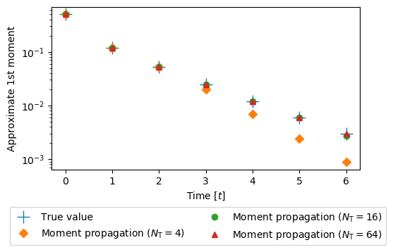
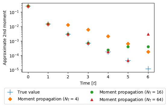
Figure 2: Moment approximations for stochastic logistic map.

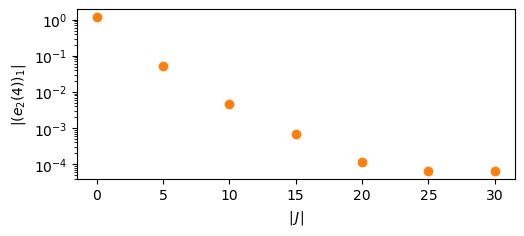
Figure 3: Error bound on moment approximations.

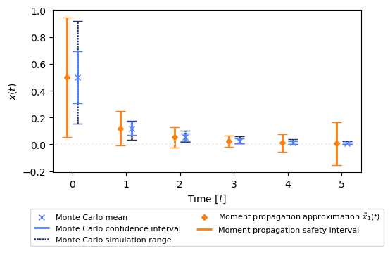
Figure 4: Tail probability analysis.

4.2 Vehicle Dynamics

Our second example is an application to autonomous driving. For safety guarantees, autonomous vehicles need to predict their future positions. One way to achieve this is set-based reachability, as advocated by Althoff and Dolan (2014). To use their method, they must consider systems with bounded disturbances and use linearization around an equilibrium, that is, they approximate a polynomial system by a linear one, using Lagrange remainders. Carleman linearization allows taking the effect of higher dimensions of the system into account more precisely than Lagrange remainders. Moreover, our approach is probabilistic, while theirs is set-based, so the two approaches give different types of guarantees.

We consider a scenario in which, at each time step, the autonomous vehicle measures its current position with some known sensor error distributions, computes moments of its current state based on this measurement and the known error distribution, and predicts its future positions (and moments) up to $t$ steps ahead in time by applying the truncated system to these moments. This process is repeated forever, leading to the framework in Figure 5.

More precisely, we consider the kinematic bicycle model of a vehicle (Kong et al., 2015), which we rewrite as the following equivalent polynomial system

$$\dot{p}_{\mathrm{x}}(t)=v(t)c(t),\quad\dot{p}_{\mathrm{y}}(t)=v(t)s(t),$$

$$\dot{\psi}(t)=\frac{v(t)}{\ell}\sin\beta,\quad\dot{v}(t)=a(t),$$

$$\dot{c}(t)=-\frac{s(t)v(t)\sin\beta}{\ell},\quad\dot{s}(t)=\frac{c(t)v(t)\sin\beta}{\ell},$$

for $t\geq 0$, where $p_{\mathrm{x}}(t)\in\mathbb{R}$ and $p_{\mathrm{y}}(t)\in\mathbb{R}$ represent the X–Y coordinates of the mass-center of the vehicle, $v(t)\in\mathbb{R}$ denotes its speed, $\psi(t)$ its inertial heading, and $a(t)\in\mathbb{R}$ its acceleration. The constants $\beta\in\mathbb{R}$ and $\ell>0$ respectively denote the angle of velocity and the distance from the vehicle’s rear axle to its mass-center. The scalars $c(t)$ and $s(t)$ are auxiliary variables that are introduced to obtain the polynomial model above from the original model of Kong et al. (2015) (which involves trigonometric terms), using the same techniques as Carothers et al. (2005).

The second-order Taylor expansion of the model above gives the following discrete-time approximation:

$$p_{\mathrm{x}}(t+\Delta) =p_{\mathrm{x}}(t)+\Delta c(t)v(t)$$

$$\quad+\frac{\Delta^{2}}{2}\biggl{(}a(t)c(t)-\frac{s(t)v^{2}(t)\sin\beta}{\ell}\biggr{)},$$

$$p_{\mathrm{y}}(t+\Delta) =p_{\mathrm{y}}(t)+\Delta s(t)v(t)$$

$$\quad+\frac{\Delta^{2}}{2}\biggl{(}a(t)s(t)+\frac{c(t)v^{2}(t)\sin\beta}{\ell}\biggr{)},$$

$$\psi(t+\Delta) =\psi(t)+\Delta\frac{v(t)}{\ell}\sin\beta+\frac{\Delta^{2}}{2}\frac{a(t)}{\ell}\sin\beta,$$

$$v(t+\Delta) =v(t)+\Delta a(t),$$

$$c(t+\Delta) =c(t)-\Delta\frac{s(t)v(t)\sin\beta}{\ell}$$

$$\quad-\frac{\Delta^{2}}{2}\biggl{(}\frac{c(t)v^{2}(t)\sin^{2}\beta}{\ell^{2}}+\frac{a(t)s(t)\sin\beta}{\ell}\biggr{)},$$

$$s(t+\Delta) =s(t)+\Delta\frac{c(t)v(t)\sin\beta}{\ell}$$

$$\quad+\frac{\Delta^{2}}{2}\biggl{(}-\frac{s(t)v^{2}(t)\sin^{2}\beta}{\ell^{2}}+\frac{a(t)c(t)\sin\beta}{\ell}\biggr{)},$$

where $\Delta>0$. To describe the evolution of the states of the vehicle at times $0,\Delta,2\Delta,\ldots$, we write this system in the form of (1). In particular, consider the discrete-time instant $t\in\mathbb{N}$ corresponding to the continuous time $t\Delta$. By letting

$$x(t) \triangleq[p_{\mathrm{x}}(t),p_{\mathrm{y}}(t),\psi(t),v(t),c(t),s(t)]^{\intercal},$$

we obtain (1) where $d_{\mathrm{S}}=3$ and the coefficients $F_{0}(t),\ldots,F_{3}(t)$ depend on $\Delta,\beta,\ell$, and $a(t)$. We consider the setting where the acceleration values $a(0),a(1),\ldots$ are independent uniform random variables over $[0.9,1]$, $\Delta=0.1$, $\beta=\pi/8$, $\ell=2.5$, and, for the initial state, $p_{\mathrm{x}}(0)$, $p_{\mathrm{y}}(0)$, $v(0)$, $\psi(0)$ are independent Gaussian random variables with mean $0$ and standard deviation $0.1$, and $c(0)=\cos(\psi(0)+\beta)$ and $s(0)=\sin(\psi(0)+\beta)$.

Figure 5: Moment propagation framework for autonomous vehicles.

4.2.1 Experimental Results.

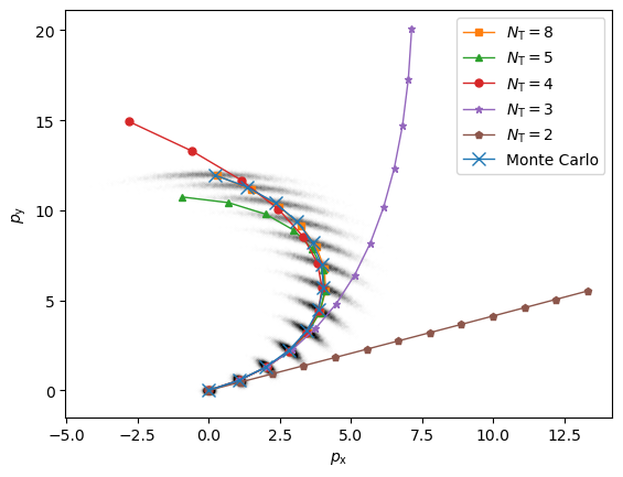
Figure 6: First moment approximation of vehicle dynamics.

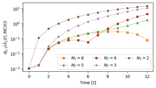
Figure 7: Distance to the mean of the empirical distribution.

Figure 6 shows the expected trajectory of the vehicle as approximated by our method for different truncation limits, as well as the empirical distribution computed by 10000 runs of Monte Carlo simulation and the mean of that distribution. Figure 7 shows the distance $d(\widetilde{x}_{1}(t),\operatorname{MC}(t))$ between $\widetilde{x}_{1}(t)$ and the mean of the empirical distribution for the same truncation limits.

Figures 6 and 7 show that larger truncation limits give systems that follow the empirical distribution better. It also shows that, for a fixed truncation limit, the distance to the empirical system grows larger with time. The only exception is around $t=6$ for $N_{\mathrm{T}}=2$, which can be explained by the fact that the trajectory of the truncated system crosses that of the empirical one. Notice that, $N_{\mathrm{T}}=8$ gives an exact computation at $t=2$, which means that the error at this point (corresponding to the horizontal line in Figure 7) is entirely induced by Monte Carlo. Therefore, it is pointless to consider errors that are of the same order as the one introduced by Monte Carlo at $t=2$.

Also note that the largest truncation limit we use in this experiment is $N_{\mathrm{T}}=8$, which makes the online computation very fast.

5 Conclusion

We have explored the problem of computing moments of discrete-time polynomial stochastic systems. Through a truncated Carleman linearization approach, we have obtained an iterative procedure for approximating the moments of the state of the system across different time instants. Furthermore, we have provided tail-probability bounds to assess the safety properties of the system.

In our analysis, we have used spherical safety regions characterized using the Euclidean norm. By changing the norm to weighted norms induced by positive-definite matrices, ellipsoidal safety regions can also be considered. We note that safety analysis for a non-ellipsoidal region can be conducted by using ellipsoids that are inside that region. Finding the largest such ellipsoid allows us to do safety analysis in the least conservative way. This is possible by solving a matrix optimization problem, which we leave for future work.

One of our future research goals is to use the approximate moments to reconstruct an approximation of the distribution of the state of the system. There exist different techniques to achieve this, as given for example by Schmüdgen (2017) or John et al. (2007).

Another direction for future work is to make the algorithm more efficient by using the symmetry of Kronecker powers to reduce the sizes of the matrices involved in the computations, which would allow us to compute even higher moments and more time steps in the future.

References

- Al-Tuwaim et al. (1998) Al-Tuwaim, M.S., Crisalle, O.D., and Svoronos, S.A. (1998). Discretization of nonlinear models using a modified Carleman linearization technique. In Proc. Amer. Contr. Conf., 3084–3088.
- Althoff and Dolan (2014) Althoff, M. and Dolan, J.M. (2014). Online verification of automated road vehicles using reachability analysis. IEEE Trans. Robotics, 30(4), 903–918.
- Amini et al. (2019) Amini, A., Sun, Q., and Motee, N. (2019). Carleman state feedback control design of a class of nonlinear control systems. In Proc. IFAC NecSys, 229–234.
- Athreya and Dai (2000) Athreya, K.B. and Dai, J. (2000). Random logistic maps. I. J. Theor. Probab., 13(2), 595–608.
- Banzhaf et al. (2018) Banzhaf, H., Dolgov, M., Stellet, J.E., and Zöllner, J.M. (2018). From footprints to beliefprints: Motion planning under uncertainty for maneuvering automated vehicles in dense scenarios. In Proc. Int. Conf. Intel. Transport. Systems, 1680–1687.
- Bellman and Richardson (1963) Bellman, R. and Richardson, J.M. (1963). On some questions arising in the approximate solution of nonlinear differential equations. Quart. Appl. Math., 20(4), 333–339.
- Bry and Roy (2011) Bry, A. and Roy, N. (2011). Rapidly-exploring random belief trees for motion planning under uncertainty. In Proc. IEEE ICRA, 723–730.
- Cacace et al. (2014) Cacace, F., Cusimano, V., Germani, A., and Palumbo, P. (2014). A Carleman discretization approach to filter nonlinear stochastic systems with sampled measurements. In Proc. IFAC World Congr., 9534–9539.
- Cacace et al. (2017) Cacace, F., Cusimano, V., Germani, A., Palumbo, P., and Papi, M. (2017). Optimal linear filter for a class of nonlinear stochastic differential systems with discrete measurements. In Proc. IEEE Conf. Dec. Control, 2807–2812.
- Carothers et al. (2005) Carothers, D.C., Parker, G.E., Sochacki, J.S., and Warne, P.G. (2005). Some properties of solutions to polynomial systems of differential equations. Electr. J. Differ. Eq., 2005(40), 1–17.
- Forets and Pouly (2017) Forets, M. and Pouly, A. (2017). Explicit error bounds for Carleman linearization. Online, https://arxiv.org/abs/1711.02552.
- Goswami and Paley (2017) Goswami, D. and Paley, D.A. (2017). Global bilinearization and controllability of control-affine nonlinear systems: A Koopman spectral approach. In Proc. IEEE Conf. Dec. Contr., 6107–6112.
- Gray and Wang (1991) Gray, H.L. and Wang, S. (1991). A general method for approximating tail probabilities. J. Am. Stat. Assoc., 86(413), 159–166.
- Hashemian and Armaou (2019) Hashemian, N. and Armaou, A. (2019). Feedback control design using model predictive control formulation and Carleman approximation method. AIChE J., 65, 1–11.
- John et al. (2007) John, V., Angelov, I., Öncül, A., and Thévenin, D. (2007). Techniques for the reconstruction of a distribution from a finite number of its moments. Chem. Eng. Sci., 62(11), 2890–2904.
- Kong et al. (2015) Kong, J., Pfeiffer, M., Schildbach, G., and Borrelli, F. (2015). Kinematic and dynamic vehicle models for autonomous driving control design. In Proc. IEEE Intell. Veh. Symp., 1094–1099.
- Laub (2005) Laub, A.J. (2005). Matrix Analysis for Scientists and Engineers. SIAM.
- Mesbahi et al. (2019) Mesbahi, A., Bu, J., and Mesbahi, M. (2019). On modal properties of the Koopman operator for nonlinear systems with symmetry. In Proc. Amer. Contr. Conf., 1918–1923.
- Rauh et al. (2009) Rauh, A., Minisini, J., and Aschemann, H. (2009). Carleman linearization for control and for state and disturbance estimation of nonlinear dynamical processes. In Proc. IFAC Conf. MMAR, 455–460.
- Schmüdgen (2017) Schmüdgen, K. (2017). The Moment Problem. Springer.
- Steeb and Wilhelm (1980) Steeb, W.H. and Wilhelm, F. (1980). Non-linear autonomous systems of differential equations and Carleman linearization procedure. J. Math. Anal. Appl., 77(2), 601–611.
- Wong (1983) Wong, W.S. (1983). Carleman linearization and moment equations of nonlinear stochastic equations. Stochastics, 9(1-2), 77–101.