D-SPIDER-SFO: A Decentralized Optimization Algorithm with Faster Convergence Rate for Nonconvex Problems

Abstract

Decentralized optimization algorithms have attracted intensive interests recently, as it has a balanced communication pattern, especially when solving large-scale machine learning problems. Stochastic Path Integrated Differential Estimator Stochastic First-Order method (SPIDER-SFO) nearly achieves the algorithmic lower bound in certain regimes for nonconvex problems. However, whether we can find a decentralized algorithm which achieves a similar convergence rate to SPIDER-SFO is still unclear. To tackle this problem, we propose a decentralized variant of SPIDER-SFO, called decentralized SPIDER-SFO (D-SPIDER-SFO). We show that D-SPIDER-SFO achieves a similar gradient computation cost—that is, $\mathcal{O}(\epsilon^{-3})$ for finding an $\epsilon$-approximate first-order stationary point—to its centralized counterpart. To the best of our knowledge, D-SPIDER-SFO achieves the state-of-the-art performance for solving nonconvex optimization problems on decentralized networks in terms of the computational cost. Experiments on different network configurations demonstrate the efficiency of the proposed method.

Introduction

Distributed optimization is a popular technique for solving large scale machine learning problems Li et al. (2014), ranging from visual object recognition Huang et al. (2017); He et al. (2016) to natural language processing Vaswani et al. (2017); Devlin et al. (2019). For distributed optimization, a set of workers form a connected computational network, and each worker is assigned a portion of the computing task. The centralized network topology, like parameter server Jianmin et al. (2016); Dean et al. (2012); Li et al. (2014); Zinkevich et al. (2010), consists of a central worker connected with all other workers. This communication mechanism could degrade the performance significantly in scenarios where the underlying network has low bandwidth or high latency Lian et al. (2017).

In contrast, the decentralized network topology offers better network load balance—as all nodes in the network only communicate with their neighbors instead of the central node—which implies that they may be able to outperform their centralized counterparts. These motivate many works on decentralized algorithms. Nedić and Ozdaglar (2009) studied distributed subgradient method for optimizing a sum of convex objective functions. Shi et al. (2014) analyzed the linear convergence rate of the ADMM in decentralized consensus optimization. Yuan, Ling, and Yin (2016) studied the convergence properties of the decentralized gradient descent method (DGD). They proved that the local solutions and the mean solution converge to a neighborhood of the global minimizer at a linear rate for strongly convex problems. Mokhtari and Ribeiro (2016) studied decentralized double stochastic averaging gradient algorithm (DSA) and Wei et al. (2015) proposed decentralized exact first-order algorithm (EXTRA). Both of these two algorithms converge to an optimal solution at a linear rate for strongly convex problems. Lian et al. (2017) studied decentralized PSGD (D-PSGD) and showed that decentralized algorithms could be faster than their centralized counterparts. Tang et al. (2018) proposed D² algorithm which is less sensitive to the data variance across workers. Scaman et al. (2018) provided two optimal decentralized algorithms, called multi-step primal-dual (MSPD) and distributed randomized smoothing (DRS), and their corresponding optimal convergence rate for convex problems in certain regimes. Assran et al. (2019) proposed Stochastic Gradient Push (SGP) and proved that SGP converges to a stationary point of smooth and nonconvex objectives at the sub-linear rate.

On the other hand, to achieve a faster convergence rate, researchers have also proposed many nonconvex optimization algorithms. Stochastic Gradient Descent (SGD) Robbins and Monro (1951) achieves an $\epsilon$-approximate stationary point with a gradient cost of $\mathcal{O}(\epsilon^{-4})$ Ghadimi and Lan (2013). To improve the convergence rate of SGD, researchers have proposed variance-reduction methods Roux, Schmidt, and Bach (2012); Defazio, Bach, and Lacoste-Julien (2014). Specifically, the finite-sum Stochastic Variance Reduced Gradient method (SVRG) Johnson and Zhang (2013); Reddi et al. (2016) and online Stochastically Controlled Stochastic Gradient method (SCSG) Lei et al. (2017) achieve a gradient cost of $\mathcal{O}(\min(m^{2/3}\epsilon^{-2},\epsilon^{-10/3}))$, where $m$ is the number of samples. SNVRG Zhou, Xu, and Gu (2018) achieves a gradient cost of $\mathcal{\widetilde{O}}(\epsilon^{-3})$, while SPIDER-SFO Fang et al. (2018) and SARAH Nguyen et al. (2017, 2019) achieve a gradient cost of $\mathcal{O}(\epsilon^{-3})$. Moreover, Fang et al. (2018) showed that SPIDER-SFO nearly achieves the algorithmic lower bound in certain regimes for nonconvex problems. Though these works have made significant progress, convergence properties of faster optimization algorithms for nonconvex problems in the decentralized settings are unclear.

In this paper, we propose decentralized SPIDER-SFO (D-SPIDER-SFO) for faster convergence rate for nonconvex problems. We theoretically analyze that D-SPIDER-SFO achieves an $\epsilon$-approximate stationary point in gradient cost of $\mathcal{O}(\epsilon^{-3})$, which achieves the state-of-the-art performance for solving nonconvex optimization problems in the decentralized settings. Moreover, this result indicates that D-SPIDER-SFO achieves a similar gradient computation cost to its centralized competitor, called centralized SPIDER-SFO (C-SPIDER-SFO). To give a quick comparison of our algorithm and other existing first-order algorithms for nonconvex optimization in the decentralized settings, we summarize the gradient cost and communication complexity of the most relevant algorithms in Table1. Table 1 shows that D-SPIDER-SFO converges faster than D-PSGD and D² in terms of the gradient computation cost. Moreover, compared with C-SPIDER-SFO, D-SPIDER-SFO reduces much communication cost on the busiest worker. Therefore, D-SPIDER-SFO can outperform C-SPIDER-SFO when the communication becomes the bottleneck of the computational network. Our main contributions are as follows.

1. We propose D-SPIDER-SFO for finding approximate first-order stationary points for nonconvex problems in the decentralized settings, which is a decentralized parallel version of SPIDER-SFO.

2. We theoretically analyze that D-SPIDER-SFO achieves the gradient computation cost of $\mathcal{O}(\epsilon^{-3})$ to find an $\epsilon$-approximate first-order stationary point, which is similar to SPIDER-SFO in the centralized network topology. To the best of our knowledge, D-SPIDER-SFO achieves the state-of-the-art performance for solving nonconvex optimization problems in the decentralized settings.

Notation: Let $\|\cdot\|$ be the vector and the matrix $\ell_{2}$ norm and $\|\cdot\|_{F}$ be the matrix Frobenius norm. $\nabla f(\cdot)$ denotes the gradient of a function $f$. Let $\mathbf{1}_{n}$ be the column vector in $\mathbb{R}^{n}$ with $1$ for all elements and $e_{i}$ be the column vector with a 1 in the $i$th coordinate and 0’s elsewhere. We denote by $f^{*}$ the optimal solution of $f$. For a matrix $A\in\mathbb{R}^{n\times n}$, let $\lambda_{i}(A)$ be the $i$-th largest eigenvalue of a matrix. For any fixed integer $j\geq i\geq 0$, let $[i:j]$ be the set $\{i,i+1,\dots,j\}$ and $\{x\}_{i:j}$ be the sequence $\{x_{i},x_{i+1},\dots,x_{j}\}$.

Table 1: Comparision of D-PSGD, D² and D-SPIDER-SFO and their centralized competitors.

Algorithm	Communication cost on	Gradient	Bounded data
	the busiest node	Computation Cost	variance among workers
C-PSGD Dekel et al. (2012)	$\mathcal{O}(n)$	$\mathcal{O}(\epsilon^{-4})$	$\times$
D-PSGD Lian et al. (2017)	$\mathcal{O}$ $($Deg$($network$))$	$\mathcal{O}(\epsilon^{-4})$	need
D2Tang et al. (2018)	$\mathcal{O}$ $($Deg$($network$))$	$\mathcal{O}(\epsilon^{-4})$	no need
C-SPIDER-SFO Fang et al. (2018)	$\mathcal{O}(n)$	$\mathcal{O}(\epsilon^{-3})$	$\times$
D-SPIDER-SFO	$\mathcal{O}$ $($Deg$($network$))$	$\mathcal{O}(\epsilon^{-3})$	no need

Basics and Motivation

Decentralized Optimization Problems

In this section, we briefly review some basics of the decentralized optimization problem. We represent the decentralized communication topology with a weighted directed graph: $(V,W)$. $V$ is the set of all computational nodes, that is, $V:=\{1,2,\dots,n\}.$ $W$ is a matrix and $W_{i,j}$ represents how much node $j$ can affect node $i$, while $W_{ij}=0$ means that node $i$ and $j$ are disconnected. Therefore, $W_{ij}\in[0,1],$ for all $i,j$. Moreover, in the decentralized optimization settings, we assume that $W$ is symmetric and doubly stochastic, which means that $W$ satisfies (i) $W_{ij}=W_{ji}$ for all $i,j$, and (ii) $\sum_{j}W_{ij}=1$ for all $i$ and $\sum_{i}W_{ij}=1$ for all $j$.

Throughout this paper, we consider the following decentralized optimization problem:

$$\min_{x\in\mathbb{R}^{N}}f(x):=\frac{1}{n}\sum_{i=1}^{n}\underbrace{\mathbb{E}_{\xi\in\mathcal{D}_{i}}F_{i}(x;\xi)}_{=:f_{i}(x)},$$ (1)

where $n$ is the number of workers, $\mathcal{D}_{i}$ is a predefined distribution of the local data for worker $i$, and $\xi$ is a random data sample. Decentralized problems require that the graph of the computational network is connected and each worker can only exchange local information with its neighbors.

In the $i$-th node, $x_{i},\xi_{i},f_{i}(x_{i}),F_{i}(x_{i};\xi_{i})$ is the local optimization variables, random sample, target function and stochastic component function. Let $\mathcal{S}$ be a subset that samples $S$ elements in the dataset. For simplicity, we denote by $\xi_{k,i}$ the subset that $i$-th node samples at iterate $k$, that is, $\nabla F_{i}(x_{k,i};\xi_{k,i})=\nabla F_{i}(x_{k,i};\mathcal{S}_{k,i})=\frac{1}{S_{k,i}}\sum_{\xi_{j}\in\mathcal{S}_{k,i}}\nabla F_{i}(x_{k,i};\xi_{j})$. In order to present the core idea more clearly, at iterate $k$, we define the concatenation of all local optimization variables, estimators of full gradients, stochastic gradients, and full gradients by matrix $X_{k},G_{k},\partial F(X_{k};\xi_{k}),\partial f(X_{k})\in\mathbb{R}^{N\times n}$ respectively:

$$X_{k} :=[x_{k,1},\ \ \cdots\ \ ,x_{k,n}],$$

$$G_{k} :=[g_{k,1},\ \ \cdots\ \ ,g_{k,n}],$$

$$\partial F(X_{k},\xi_{k}) :=[\nabla F_{1}(x_{k,1};\xi_{k,1}),\ \ \cdots\ \ ,\nabla F_{n}(x_{k,n};\xi_{k,n})],$$

$$\partial f(X_{k}) :=[\nabla f_{1}(x_{k,1}),\ \ \cdots\ \ ,\nabla f_{n}(x_{k,n})].$$

In general, at iterate $k$, let the stepsize be $\eta_{k}$. We define $\eta_{k}V_{k}$ as the update, where $V_{k}\in\mathbb{R}^{N\times n}$. Therefore, we can view the update rule as:

$$X_{k+1}\leftarrow X_{k}W-\eta_{k}V_{k}.$$ (2)

D-SPIDER-SFO

In this section, we introduce the basic settings, assumptions, and the flow of D-SPIDER-SFO in the first subsection. Then, we compare D-SPIDER-SFO with D-PSGD and D² in a special scenario to show our core idea. In the final subsection, we propose the error-bound theorems for finding an $\epsilon$-approximate first-order stationary point.

Algorithm 1 D-SPIDER-SFO on the $i$th node

Input: Require initial point $X_{0}$, weighted matrix $W$, number of iterations $K$, learning rate $\eta$, constant $q$, and two sample sizes $S^{(1)}$ and $S^{(2)}$

Initialize: $X_{-1}=X_{0}$, $G_{-1}$ = $0$

for $k=0,\dots,K-1$ do

     if mod$(k,q)=0$ then

         Draw $S^{(1)}$ samples and compute the stochastic gradient $\nabla F_{i}(x_{k,i};\mathcal{S}^{(1)}_{k,i})$

         $g_{k,i}=\nabla F_{i}(x_{k,i};\mathcal{S}^{(1)}_{k,i})$

         $x_{k+\frac{1}{2},i}=2x_{k,i}-x_{k-1,i}-\eta(g_{k,i}-g_{k-1,i})$

     else

         Draw $S^{(2)}$ samples, and compute two stochastic gradient $\nabla F_{i}(x_{k,i};\mathcal{S}^{(2)}_{k,i})$ and $\nabla F_{i}(x_{k-1,i};\mathcal{S}^{(2)}_{k,i})$

         $g_{k,i}=\nabla F_{i}(x_{k,i};\mathcal{S}^{(2)}_{k,i})-\nabla F_{i}(x_{k-1,i};\mathcal{S}^{(2)}_{k,i})+g_{k-1,i}$

         $x_{k+\frac{1}{2},i}=2x_{k,i}-x_{k-1,i}-\eta(\nabla F_{i}(x_{k,i};\mathcal{S}^{(2)}_{k,i})-\nabla F_{i}(x_{k-1,i};\mathcal{S}^{(2)}_{k,i}))$

     end if

     $x_{k+1,i}=\sum_{j=1}^{n}W_{j,i}x_{k+\frac{1}{2},j}$

end for

Return $\widetilde{x}=\frac{X_{K}\mathbf{1}_{n}}{n}$

Settings and Assumptions

In this subsection, we introduce the formal definition of an $\epsilon$-approximate first-order stationary point and commonly used assumptions for decentralized optimization problems. Moreover, we briefly introduce the key steps at iterate $k$ for worker $i$ in D-SPIDER-SFO algorithm.

Definition 1.

We call $\widetilde{x}\in\mathbb{R}^{N}$ an $\epsilon$-approximate first-order stationary point, if

$$\|\nabla f(\widetilde{x})\|\leq\epsilon.$$ (3)

Assumption 1.

We make the following commonly used assumptions for the convergence analysis.

1. Lipschitz gradient: All local loss functions $f_{i}(\cdot)$ have $L$-Lipschitzian gradients.

2. Average Lipschitz gradient: In each fixed node $i$, the component function $F_{i}(x_{i};\xi_{i})$ has an average L-Lipschitz gradient, that is,

   $$\mathbb{E}\|\nabla F_{i}(x;\xi_{i})-\nabla F_{i}(y;\xi_{i})\|^{2}\leq L^{2}\|x-y\|^{2},\forall x,y.$$

3. Spectral gap: Given the symmetric doubly stochastic matrix $W$. Let the eigenvalues of $W\in\mathbb{R}^{n\times n}$ be $\lambda_{1}\geq\lambda_{2}\geq\cdots\geq\lambda_{n}$. We denote by $\lambda$ the second largest value of the set of eigenvalues, i.e.,

   $$\lambda=\max_{i\in\{2,\cdots,n\}}\lambda_{i}=\lambda_{2}.$$

   We assume $\lambda<1$ and $\lambda_{n}>-\frac{1}{3}$.

4. Bounded variance: Assume the variance of stochastic gradient within each worker is bounded, which implies there exists a constant $\sigma$, such that

   $$\mathbb{E}_{\xi\sim\mathcal{D}_{i}}\|\nabla F_{i}(x;\xi)-\nabla f_{i}(x)\|^{2}\leq\sigma^{2},\forall i,\forall x.$$

5. (For D-PSGD Algorithm only) Bounded data variance among workers: Assume the variance of full gradient among all workers is bounded, which implies that there exists a constant $\zeta$, such that

   $$\mathbb{E}_{i\sim\mathcal{U}([n])}\|\nabla f_{i}(x)-\nabla f(x)\|^{2}\leq\zeta^{2},\forall i,\forall x.$$

Remark 1.

The eigenvalues of $W$ measure the speed of information spread across the network Lian et al. (2017). D-SPIDER-SFO requires $\lambda_{2}<1$ and $\lambda_{n}>-\frac{1}{3}$, which is the same as the assumption in D² Tang et al. (2018), while D-PSGD only needs the former condition. D-PSGD needs bounded data variance among workers assumption additionally, as it is sensitive to such data variance.

D-SPIDER-SFO algorithm is a synchronous decentralized parallel algorithm. Each node repeats these four key steps at iterate $k$ concurrently:

1. Each node computes a local stochastic gradient on their local data. When $\mod(k,q)\not=0$, all nodes compute $\nabla F_{i}(x_{k,i};\mathcal{S}^{(2)}_{k,i})$ and $\nabla F_{i}(x_{k-1,i};\mathcal{S}^{(2)}_{k,i})$ using the local models at both iterate $k$ and the last iterate; otherwise, they compute $\nabla F_{i}(x_{k,i};\mathcal{S}^{(1)}_{k,i})$.

2. Each node updates its local estimator of the full gradient $g_{k,i}$. When $\mod(k,q)\not=0$, all nodes compute $g_{k,i}\leftarrow\nabla F_{i}(x_{k,i};\mathcal{S}^{(2)}_{k,i})-\nabla F_{i}(x_{k-1,i};\mathcal{S}^{(2)}_{k,i})+g_{k-1,i}$; else they compute $g_{k,i}\leftarrow\nabla F_{i}(x_{k,i};\mathcal{S}^{(1)}_{k,i})$.

3. Each node updates their local model. When $\mod(k,q)\not=0$, all nodes compute $x_{k+\frac{1}{2},i}\leftarrow 2x_{k,i}-x_{k-1,i}-\eta(\nabla F_{i}(x_{k,i};\mathcal{S}^{(2)}_{k,i})-\nabla F_{i}(x_{k-1,i};\mathcal{S}^{(2)}_{k,i}))$; else they compute $x_{k+\frac{1}{2},i}\leftarrow 2x_{k,i}-x_{k-1,i}-\eta(g_{k,i}-g_{k-1,i})$.

4. When meeting the synchronization barrier, each node takes weighted average with its and neighbors’ local optimization variables: $x_{k+1,i}=\sum_{j=1}^{n}W_{j,i}x_{k+\frac{1}{2},j}.$

To understand D-SPIDER-SFO, we consider the update rule of global optimization variable $\frac{X_{k}\mathbf{1}_{n}}{n}$. Let $k_{0}=\lfloor k/q\rfloor\cdot q$. For convenience, we define

$$\overline{\Delta}_{k} =\frac{(X_{k+1}-X_{k})\mathbf{1}_{n}}{n}=\frac{1}{n}\sum_{i=1}^{n}(x_{k+1,i}-x_{k,i}),$$

$$\overline{H}_{k}(X) =\partial F(X;\xi_{k})\frac{\mathbf{1}_{n}}{n}=\frac{1}{n}\sum_{i=1}^{n}\nabla F_{i}(x_{i};\xi_{k,i}),$$

where $\xi_{k}$ denotes the samples at the $k$-th iterate. Therefore,

$$\overline{\Delta}_{k}= \overline{\Delta}_{k-1}-\eta(\overline{H}_{k}(X_{k})-\overline{H}_{k}(X_{k-1}))$$

$$= -\eta\overline{H}_{k_{0}}(X_{k_{0}})-\eta\sum_{s=k_{0}+1}^{k}(\overline{H}_{s}(X_{s})-\overline{H}_{s}(X_{s-1})).$$

As for centralized SPIDER-SFO, we have

$$x_{k+1}-x_{k}= -\eta_{k}(\nabla F(x_{k};\xi_{k})-\nabla F(x_{k-1};\xi_{k})+v_{k-1})$$

$$= -\eta_{k_{0}}\nabla F(x_{k_{0}};\xi_{k_{0}})-\sum_{s=k_{0}+1}^{k}\eta_{s}(\nabla F(x_{s};\xi_{s})-\nabla F(x_{s-1};\xi_{s})).$$

Remark 2.

Nguyen et al. propose SARAH for (strongly) convex optimization problems. SPIDER-SFO adopts a similar recursive stochastic gradient update framework and nearly matches the algorithmic lower bound in certain regimes for nonconvex problems. Moreover, Wang et al. [2] propose SpiderBoost and show that SpiderBoost, a variant of SPIDER-SFO with fixed step size, achieves a similar convergence rate to SPIDER-SFO for nonconvex problems. Inspired by these algorithms, we propose decentralized SPIDER-SFO (D-SPIDER-SFO). As we can see, the update rule of D-SPIDER-SFO is similar to its centralized counterpart with fixed step size.

Core Idea

The convergence property of decentralized parallel stochastic algorithms is related to the variance of stochastic gradients and the data variance across workers. In this subsection, we present in detail the underlying idea to reduce the gradient complexity behind the algorithm design.

The general update rule (2) shows that $\mathbb{E}[\left\|V_{k}\right\|^{2}_{F}]$ affects the convergence, especially when we approach a solution. For showing the improvement of D-SPIDER-SFO, we will compare the upper bound of $\mathbb{E}[\|V_{k}\|^{2}_{F}]$ of three algorithms, which are D-PSGD, D², and D-SPIDER-SFO.

The update rule of D-PSGD is $X_{k+1}=X_{k}W-\eta\partial F(X_{k};\xi_{k})$, that is, $V_{k}=\partial F(X_{k};\xi_{k})$. Then, we have

$$\mathbb{E}\|\partial F(X_{k};\xi_{k})\|_{F}^{2}\leq 4\mathbb{E}\|\partial F(X_{k};\xi_{k})-\partial f(X_{k})\|_{F}^{2}+4\mathbb{E}\left\|\partial f(X_{k})-\partial f\left(\frac{X_{k}\mathbf{1}_{n}}{n}\mathbf{1}_{n}^{T}\right)\right\|_{F}^{2}$$

$$+4\mathbb{E}\left\|\partial f\left(\frac{X_{k}\mathbf{1}_{n}}{n}\mathbf{1}_{n}^{T}\right)-\nabla f\left(\frac{X_{k}\mathbf{1}_{n}}{n}\right)\mathbf{1}_{n}^{T}\right\|_{F}^{2}+4\mathbb{E}\left\|\nabla f\left(\frac{X_{k}\mathbf{1}_{n}}{n}\right)\mathbf{1}_{n}^{T}\right\|_{F}^{2}$$

$$\leq 4n\sigma^{2}+4n\zeta^{2}+4L^{2}\sum_{i=1}^{n}\left\|x_{k,i}-\frac{X_{k}\mathbf{1}_{n}}{n}\right\|^{2}+4\mathbb{E}\left\|\nabla f\left(\frac{X_{k}\mathbf{1}_{n}}{n}\right)\mathbf{1}_{n}^{T}\right\|_{F}^{2}.$$

Moreover, the update rule of D² is $X_{k+1}=\left[2X_{k}-X_{k-1}-\eta(\partial F(X_{k};\xi_{k})-\partial F(X_{k-1};\xi_{k-1}))\right]W$. For convenience, we define $Q_{k}=\frac{X_{k}-X_{k-1}}{\eta}$. Therefore, we can conclude the upper bound of $\mathbb{E}\|V_{k}\|_{F}^{2}$.

$$\mathbb{E}\left\|V_{k}\right\|^{2}_{F}= \mathbb{E}\left\|\left[-Q_{k}+(\partial F(X_{k};\xi_{k})-\partial F(X_{k-1};\xi_{k-1}))\right]W\right\|^{2}_{F}$$

$$\leq 2\mathbb{E}\left\|Q_{k}\right\|^{2}_{F}+2\mathbb{E}\|\partial F(X_{k};\xi_{k})-\partial F(X_{k-1};\xi_{k-1})\|^{2}_{F}$$

$$\leq 2\mathbb{E}\left\|Q_{k}\right\|^{2}_{F}+6\mathbb{E}\|\partial F(X_{k};\xi_{k})-\partial f(X_{k})\|^{2}_{F}$$

$$+6\mathbb{E}\|\partial F(X_{k-1};\xi_{k-1})-\partial f(X_{k-1})\|^{2}_{F}+6\mathbb{E}\|\partial f(X_{k})-\partial f(X_{k-1})\|^{2}_{F}$$

$$\leq \frac{2}{\eta^{2}}\sum_{i=1}^{n}\mathbb{E}\left\|x_{k,i}-x_{k-1,i}\right\|^{2}+6\sum_{i=1}^{n}\mathbb{E}\|\nabla F_{i}(x_{k,i};\xi_{k,i})-\nabla f_{i}(x_{k,i})\|^{2}$$

$$+6\sum_{i=1}^{n}\mathbb{E}\|\nabla F_{i}(x_{k-1,i};\xi_{k-1,i})-\nabla f_{i}(x_{k-1,i})\|^{2}+6\sum_{i=1}^{n}\mathbb{E}\|\nabla f_{i}(x_{k,i})-\nabla f_{i}(x_{k-1,i})\|^{2}$$

$$\leq 2\left(\eta^{-2}+3L^{2}\right)\sum_{i=1}^{n}\mathbb{E}\|x_{k,i}-x_{k-1,i}\|^{2}+12n\sigma^{2}.$$

Since the update rule of D-SPIDER-SFO has two different patterns, we discuss them seperately. If $\mod(k,q)\not=0$, we have $V_{k}=[-Q_{k}-(\partial F(X_{k};\xi_{k})-\partial F(X_{k-1};\xi_{k}))]W$.

$$\mathbb{E}\left\|V_{k}\right\|^{2}_{F}= \mathbb{E}\left\|\left[Q_{k}+(\partial F(X_{k};\xi_{k})-\partial F(X_{k-1};\xi_{k}))\right]W\right\|^{2}_{F}$$

$$\leq 2\mathbb{E}\left\|Q_{k}\right\|^{2}_{F}+2\mathbb{E}\|\partial F(X_{k};\xi_{k})-\partial F(X_{k-1};\xi_{k})\|^{2}_{F}$$

$$\leq \frac{2}{\eta^{2}}\sum_{i=1}^{n}\mathbb{E}\left\|x_{k,i}-x_{k-1,i}\right\|^{2}+2\sum_{i=1}^{n}\mathbb{E}\|\nabla F_{i}(x_{k,i};\xi_{k,i})-\nabla F_{i}(x_{k-1,i};\xi_{k,i})\|^{2}_{F}$$

$$\leq 2\left(\eta^{-2}+L^{2}\right)\sum_{i=1}^{n}\mathbb{E}\|x_{k,i}-x_{k-1,i}\|^{2}.$$

If $\mod(k,q)=0$ and $k>0$, we have $V_{k}=[-Q_{k}-(\partial F(X_{k};\xi_{k})-G_{k-1})]W$. Let $k_{0}=k-q$, and we have

$$\mathbb{E}\left\|V_{k}\right\|^{2}_{F}= \mathbb{E}\left\|\left[-Q_{k}-(\partial F(X_{k};\xi_{k})-G_{k-1})\right]W\right\|^{2}_{F}$$

$$\leq 2\mathbb{E}\|Q_{k}\|^{2}_{F}+2\mathbb{E}\|\partial F(X_{k};\xi_{k})-G_{k-1}\|^{2}_{F}$$

$$\leq 2\mathbb{E}\|Q_{k}\|^{2}_{F}+4\mathbb{E}\|\partial F(X_{k};\xi_{k})-\partial F(X_{k_{0}};\xi_{k_{0}})\|^{2}_{F}+4\mathbb{E}\left\|\sum_{j=k_{0}}^{k-2}(\partial F(X_{j+1};\xi_{j+1})-\partial F(X_{j};\xi_{j+1})\right\|^{2}_{F},$$ (4)

where

$$G_{k-1}= \sum_{j=k_{0}}^{k-2}\left(\partial F(X_{j+1};\xi_{j+1})-\partial F(X_{j};\xi_{j+1})\right)+\partial F(X_{k_{0}};\xi_{k_{0}}).$$

Assume that for any $j\in[k_{0}:k]$, $X_{j}$ has achieved the optimum $X^{*}:=x^{*}\mathbf{1}_{n}^{T}$ with all local models equal to the optimum $x^{*}$. Then, $\mathbb{E}[\left\|V_{k}\right\|_{F}^{2}]$ of D-PSGD, and D², is bounded by $\mathcal{O}(\sigma^{2}+\zeta^{2})$, $\mathcal{O}(\sigma^{2})$, which is similar to Tang et al. (2018). For convenience, considering the finite-sum case, if we set the batch size $S_{1}$ equal to the size $m$ of the dataset, that is, we compute the full gradient at iteration $k$ and $k_{0}$. Moreover, as for any $j\in[k_{0}:k]$, $X_{j}=X^{*}$, then each term of (Core Idea) is zero, that is, $\mathbb{E}[\left\|V_{k}\right\|_{F}^{2}]$ is bounded by zero. D-SPIDER-SFO will stop at the optimum, while D-PSGD and D² will escape from the optimum because of the variance of stochastic gradients or data variance across workers. If we need D² stops at the optimum, D² should compute the full gradient at each iteration, which is similar to EXTRA Wei et al. (2015), while D-SPIDER-SFO needs to compute full gradient per $q$ iteration. This is the key ingredient for the superior performance of D-SPIDER-SFO. By this sight, D-SPIDER-SFO achieves a faster convergence rate. In the following analysis, we show that the gradient cost of D-SPIDER-SFO is $\mathcal{O}(\frac{1}{\epsilon^{3}})$.

Convergence Rate Analysis

In this subsection, we analyze the convergence properties of the D-SPIDER-SFO algorithm. We propose the error bound of the gradient estimation in Lemma 1, which is critical in convergence analysis. Then, based on Lemma 1, we present the upper bound of gradient cost for finding an $\epsilon$ approximate first-order stationary point, which is the state-of-the-art for decentralized nonconvex optimization problems.

Before analyzing the convergence properties, we consider the update rule of global optimization variables as follows,

$$\frac{X_{k+1}\mathbf{1}_{n}}{n}=\frac{(X_{k}W-\eta V_{k})\mathbf{1}_{n}}{n}=\frac{(X_{k}-\eta V_{k})\mathbf{1}_{n}}{n}.$$

To analyze the convergence rate of D-SPIDER-SFO, we conclude the following Lemma 1 which bounds the error of the gradient estimator $\frac{V\mathbf{1}_{n}}{n}$.

Lemma 1.

Under the Assumption 1, we have

$$\frac{1}{K}\sum_{k=0}^{K-1}\mathbb{E}\left\|\frac{\partial f(X_{k})\mathbf{1}_{n}}{n}-\frac{V_{k}\mathbf{1}_{n}}{n}\right\|^{2}$$

$$\leq \frac{12C_{1}L^{2}q}{KnDS_{2}}\mathbb{E}\|X_{1}\|^{2}_{F}+\left(\frac{72C_{2}\eta^{4}L^{4}q^{2}}{KDS^{2}_{2}}+\frac{3qL^{2}\eta^{2}}{KS_{2}}\right)\sum_{k=1}^{K-1}\mathbb{E}\left\|\frac{V_{k-1}\mathbf{1}_{n}}{n}\right\|^{2}+\left(1+\frac{192C_{2}L^{2}\eta^{2}}{nDS_{1}}\right)\frac{\sigma^{2}}{S_{1}}.$$

where

$$C_{1} =\max\left\{\frac{1}{1-|b_{n}|^{2}},\frac{1}{(1-\lambda_{2})^{2}}\right\},$$

$$C_{2} =\max\left\{\frac{\lambda_{n}^{2}}{(1-|b_{n}|^{2})},\frac{\lambda_{2}^{2}}{(1-\sqrt{\lambda_{2}})^{2}(1-\lambda_{2})}\right\},$$

$$b_{n} =\lambda_{n}-\sqrt{\lambda_{n}^{2}-\lambda_{n}},$$

$$D =1-\frac{48C_{2}q\eta^{2}L^{2}}{S_{2}}.$$

In Appendix, we will give the upper bound of $\mathbb{E}\|X_{1}\|^{2}_{F}$. Lemma 1 shows that the error bound of the gradient estimator is related to the second moment of $\left\|\frac{X_{k}\mathbf{1}_{n}}{n}\right\|$. Then, we give the analysis of the convergence rate. W.l.o.g., we assume the algorithm starts from $0$, that is $X_{0}=0$, and define $\zeta_{0}=\frac{1}{n}\sum_{i=1}^{n}\|\nabla f_{i}(\mathbf{0})-\nabla f(\mathbf{0})\|$.

Theorem 1.

For the online case, set parameters $S_{1}$, $S_{2}$, $\eta$, and $q$ as constants, and $C_{1},C_{2}$, and $D$ as in Lemma 1. Then, under the Assumption 1, for Algorithm 1, we have

$$\frac{1}{K}\sum_{k=1}^{K}\mathbb{E}\left\|\nabla f\left(\frac{X_{k}\mathbf{1}_{n}}{n}\right)\right\|^{2}+\frac{M}{K}\sum_{k=0}^{K-1}\mathbb{E}\left\|\frac{V_{k}\mathbf{1}_{n}}{n}\right\|^{2}$$

$$\leq \frac{2\mathbb{E}[f(\frac{X_{0}\mathbf{1}_{n}}{n})-f^{*}]}{\eta K}+\left(1+\frac{32C_{2}L^{2}\eta^{2}}{nqD}+\frac{192C_{2}L^{2}\eta^{2}}{nS_{2}D}\right)\frac{2\sigma^{2}}{S_{1}}+\frac{3\eta^{2}}{K}\left(\frac{4L^{2}C_{1}}{D}+\frac{24L^{2}C_{1}q}{DS_{2}}\right)(\sigma^{2}+\zeta_{0}^{2}+\|\nabla f(0)\|^{2}),$$

where

$$M:=1-L\eta-\frac{6qL^{2}\eta^{2}}{S_{2}}\left[1+\frac{4C_{2}L^{2}\eta^{2}}{D}\left(1+\frac{6q}{S_{2}}\right)\right].$$

By appropriately specifying the batch size $S_{1},S_{2}$, the step size $\eta$, and the parameter $q$, we reach the following corollary. In the online learning case, we let the input parameters be

$$S_{1}=\frac{\sigma^{2}}{\epsilon^{2}},S_{2}=\frac{\sigma}{\epsilon},q=\frac{\sigma}{\epsilon},$$ (5)

$$\eta<\min\left(\frac{-1+\sqrt{13}}{12L},\frac{1}{4\sqrt{3C_{2}}L}\right).$$ (6)

Corollary 1.

Set the parameters $S_{1},S_{2},q,\eta$ as in (5) and (6), and set $K=\lfloor\frac{l}{\epsilon^{2}}\rfloor+1$. Then under the Assumption 1, running Algorithm 1 for $K$ iterations, we have

$$\frac{1}{K}\sum_{k=0}^{K-1}\mathbb{E}\left\|\nabla f\left(\frac{X_{k}\mathbf{1}}{n}\right)\right\|^{2}\leq 3\epsilon^{2}+\frac{448C_{2}L^{2}\eta^{2}\epsilon^{3}}{nD\sigma},$$

where

$$l:= \frac{2\mathbb{E}[f(0)-f^{*}]}{\eta}+\frac{84C_{1}L^{2}\eta^{2}}{D}(\sigma^{2}+\zeta_{0}^{2}+\|\nabla f(0)\|^{2}).$$

The gradient cost is bounded by $2l\sigma\epsilon^{-3}+2\sigma^{2}\epsilon^{-2}$.

Remark 3.

Corollary 1 shows that measured by gradient cost, D-SPIDER-SFO achieves the convergence rate of $\mathcal{O}(\epsilon^{-3})$, which is similar to its centralized counterparts. Due to properties of decentralized optimization problems, the coefficient in Corollary 1 of the term $\epsilon^{-3}$ depends on the network topology $W$ and the data variance among workers $\zeta^{2}$ in addition, while compared with the centralized competitor Fang et al. (2018). Although the differences exist, we conduct experiments to show that D-SPIDER-SFO converges with a similar speed to C-SPIDER-SFO.

Experiments

In this section, we conduct extensive experiments to validate our theory. We introduce our experiment settings in the first subsection. Then in the second subsection, we conduct the experiments to demonstrate that D-SPIDER-SFO can get a similar convergence rate to C-SPIDER-SFO and converges faster than D-PSGD and D². Moreover, we validate that D-SPIDER-SFO outperforms its centralized counterpart, C-SPIDER-SFO, on the networks with low bandwidth or high latency. In the final, we show that D-SPIDER-SFO is robust to the data variance among workers. The code of D-SPIDER-SFO is available on GitHub at https://github.com/MIRALab-USTC/D-SPIDER-SFO.

Experiment setting

Datasets and models We conduct our experiments on the image classification task. In our experiments, we train our models on CIFAR-10 Krizhevsky and Hinton (2009). The CIFAR-10 dataset consists of 60,000 32x32 color images in 10 classes when the training set has 50,000 images. For image classification, we train two convolution neural network models on CIFAR-10. The first one is LeNet5 Lecun et al. (1998), which consists of a 6-filter $5\times 5$ convolution layer, a $2\times 2$ max-pooling layer, a 16-filter $5\times 5$ convolution layer and two fully connected layers with 120, 84 neurons respectively. The second one is ResNet-18 He et al. (2015).
Implementations and setups We implement our code on framework PyTorch. All implementations are compiled with PyTorch1.3 with gloo. We conduct experiments both on the CPU server and GPU server. CPU cluster is a machine with four CPUs, each of which is an Intel(R) Xeon(R) Gold 6154 CPU @ 3.00GHz with 18 cores. GPU server is a machine with 8 GPUs, each of which is a Nvidia GeForce GTX 2080Ti. In the experiments, we use the ring network topology, seeing each core or GPU as a node, with corresponding symmetric doubly stochastic matrix $W$ in the form of

$$W=\left(\begin{matrix}1/2&1/4&&&&1/4\\ 1/4&1/2&1/4&&&\\ &1/4&1/2&\ddots&&\\ &&\ddots&\ddots&1/4&&\\ &&&1/4&1/2&1/4\\ 1/4&&&&1/4&1/2\end{matrix}\right)\in\mathbb{R}^{n\times n}.$$

Experiments of D-SPIDER-SFO

To show that D-SPIDER-SFO can get a similar convergence rate to its centralized version, we choose the computational complexity as metrics instead of the wall clock speed. In the experiments of training LeNet5, for D-PSGD and D², we use the constant learning rate $\frac{\eta_{0}}{\sqrt{K/n}}$ and tune $\eta_{0}$ from $\{0.1,0.05,0.01,0.005,0.001\}$ and set the batch size $16$ for each node, where $K$ is the number of iterates and $n$ is the number of workers. For D-SPIDER-SFO and C-SPIDER-SFO, we set $S_{1}=256,S_{2}=16,q=16$ for each node, and tune the learning rate from $\{0.1,0.05,0.01,0.005,0.001\}$. When we conduct experiments on ResNet-18, for D-PSGD and D², we tune $\eta_{0}$ from $\{0.03,0.01,0.003,0.001,0.0003\}$, and also tune the learning rate of D-SPIDER-SFO and C-SPIDER-SFO from the same set $\{0.03,0.01,0.003,0.001,0.0003\}$. We conduct experiments on a computational network with eight nodes. Due to the space limitation, we show the experiments of training convolutional neural network models, LetNet5 and ResNet-18, on 8 GPUs in this paper and list the experiments on the CPU cluster in Supplement Material.

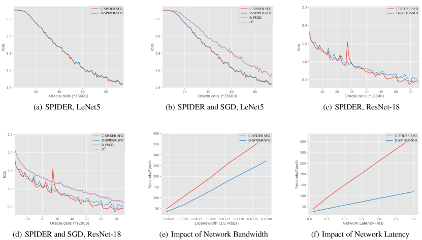
Figure 1: In the experiments, we train two convolutional neural network, LeNet5 and ResNet18. Fig. 1(a) and 1(c) are the comparisons between D-SPIDER-SFO and C-SPIDER-SFO. Fig. 1(b) and 1(d) are the comparisons between D-SPIDER-SFO, C-SPIDER-SFO, D-PSGD, and D². Fig. 1(e) and 1(d) show the impact of the bandwidth and latency.

The gradient computation cost of both D-PSGD and D² is $\mathcal{O}(\epsilon^{-4})$ for finding an $\epsilon$ approximated stationary point, while D-SPIDER-SFO achieves $\mathcal{O}(\epsilon^{-3})$. Figure 1(b) and 1(d) validates our theoretical analysis and shows that D-SPIDER-SFO converges faster than D-PSGD and D². Moreover, figure 1(a) and 1(c) also shows that D-SPIDER-SFO achieves a similar convergence rate to its centralized competitor.

As the decentralized network has more balanced communication patterns, D-SPIDER-SFO should outperform its centralized counterpart, when the communication becomes the bottleneck of the computational network. To demonstrate the above statement, we use the wall clock time as the metrics. In this experiment, we train LeNet5 on a cluster with 8 GPUs. We adopt the same parameters and experiment settings as what we use to train LeNet5. We use the tc command to control the bandwidth and latency of the network. Figure 1(e) and 1(f) shows the wall clock time to finish one epoch on different network configurations. When the bandwidth becomes smaller, or the latency becomes higher, D-SPIDER-SFO can be even one order of magnitude faster than its centralized counterpart. The experiments demonstrate that the balanced communication pattern improves the efficiency of D-SPIDER-SFO.

Tang et al. (2018) proposed D² algorithm is less sensitive to the data variance across workers. From the theoretical analysis, D-SPIDER-SFO is also robust to that variance. The experiments demonstrate the statement and show that D-SPIDER-SFO converges faster than D² when the data variance across workers is maximized.

We follow the method proposed in Tang et al. (2018) to create a data distribution with large data variance for the comparison between D-SPIDER-SFO and D². We conduct the experiments on a server with 5 GPUs and choose the computational complexity as metrics. Each worker only has access to two classes of the whole dataset, called the unshuffled case, and we tune the learning rate of D² as before.

Figure 2(a) shows that D-PSGD does not converge in the unshuffled case, which is consistent with the original work Tang et al. (2018). Figure 2(b) shows that D-SPIDER-SFO converges faster than D², and even it has a similar computing complexity as its centralized implementation. The experiments demonstrate the theoretical statement that D-SPIDER-SFO is robust to the data variance across workers.

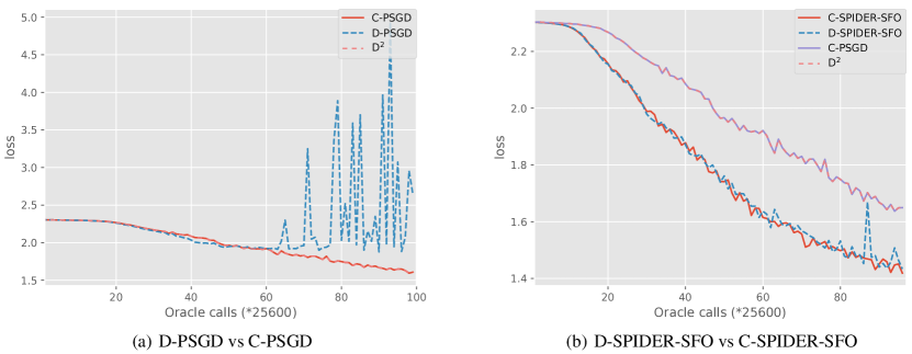
Figure 2: Fig. 2(a) is the comparison between D-PSGD and its centralized parallel version when the data is unshuffled. Fig. 2(b) is the comparison between D-SPIDER-SFO with its centralized counterpart when the data is unshuffled.

Conclusion

In this paper, we propose D-SPIDER-SFO as a decentralized parallel variant of SPIDER-SFO for a faster convergence rate for nonconvex problems. We theoretically analyze that D-SPIDER-SFO achieves an $\epsilon$-approximate stationary point in the gradient cost of $\mathcal{O}(\epsilon^{-3})$. To the best of our knowledge, D-SPIDER-SFO achieves the state-of-the-art performance for solving nonconvex optimization problems on decentralized networks. Experiments on different network configurations demonstrate the efficiency of the proposed method.

D-SPIDER-SFO: A Decentralized Optimization Algorithm with Faster Convergence Rate for Nonconvex Problems

Supplementary Material

This is the supplementary material of the paper ”D-SPIDER-SFO: A Decentralized Optimization Algorithm with Faster Convergence Rate for Nonconvex Problems”. We provide the proof to all theoretical results in this paper in this section. To help readers understand the proof, we list the necessary assumptions, which is the same as that in the main submission.

Assumption 1.

We make the following commonly used assumptions for the convergence analysis.

1. Lipschitz gradient: All local loss functions $f_{i}(\cdot)$ have $L$-Lipschitzian gradients.

2. Average Lipschitz gradient: In each fixed node $i$, the component function $F_{i}(x_{i};\xi_{i})$ has an average L-Lipschitz gradient, that is,

   $$\mathbb{E}\|\nabla F_{i}(x;\xi_{i})-\nabla F_{i}(y;\xi_{i})\|^{2}\leq L^{2}\|x-y\|^{2},\forall x,y.$$

3. Spectral gap: Given the symmetric doubly stochastic matrix $W$. Let the eigenvalues of $W\in\mathbb{R}^{n\times n}$ be $\lambda_{1}\geq\lambda_{2}\geq\cdots\geq\lambda_{n}$. We denote by $\lambda$ the second largest value of the set of eigenvalues, i.e.,

   $$\lambda=\max_{i\in\{2,\cdots,n\}}\lambda_{i}=\lambda_{2}.$$

   We assume $\lambda<1$ and $\lambda_{n}>-\frac{1}{3}$.

4. Bounded variance: Assume the variance of stochastic gradient within each worker is bounded, which implies there exists a constant $\sigma$, such that

   $$\mathbb{E}_{\xi\sim\mathcal{D}_{i}}\|\nabla F_{i}(x;\xi)-\nabla f_{i}(x)\|^{2}\leq\sigma^{2},\forall i,\forall x.$$

5. (For D-PSGD Algorithm only) Bounded data variance among workers: Assume the variance of full gradient among all workers is bounded, which implies that there exists a constant $\zeta$, such that

   $$\mathbb{E}_{i\sim\mathcal{U}([n])}\|\nabla f_{i}(x)-\nabla f(x)\|^{2}\leq\zeta^{2},\forall i,\forall x.$$

Notation: Let $\|\cdot\|$ be the vector and the matrix $\ell_{2}$ norm and $\|\cdot\|_{F}$ be the matrix Frobenius norm. $\nabla f(\cdot)$ denotes the gradient of a function $f$. Let $\mathbf{1}_{n}$ be the column vector in $\mathbb{R}^{n}$ with $1$ for all elements and $e_{i}$ be the column vector with a 1 in the $i$th coordinate and 0’s elsewhere. We denote by $f^{*}$ the optimal solution of $f$. For a matrix $A\in\mathbb{R}^{n\times n}$, let $\lambda_{i}(A)$ be the $i$-th largest eigenvalue of a matrix. For any fixed integer $j\geq i\geq 0$, let $[i:j]$ be the set $\{i,i+1,\dots,j\}$ and $\{x\}_{i:j}$ be the sequence $\{x_{i},x_{i+1},\dots,x_{j}\}$.

Basics

Consider the update rule:

$$X_{k+1}=\left\{\begin{aligned} &[2X_{k}-X_{k-1}-\eta(\partial F(X_{k};\xi_{k})-\partial F(X_{k-1};\xi_{k}))]W\qquad\mod(k,q)\not=0,\\ &[2X_{k}-X_{k-1}-\eta(\partial F(X_{k};\xi_{k})-G_{k-1})]W\qquad\mod(k,q)=0.\end{aligned}\right.$$ (7)

Since $W$ is symmetric, we have $W=P\operatorname*{Diag\,}(\lambda(W))P^{T}$. Then applying the decomposition to the update rule (7), and we have:
If $\mod(k,q)\not=0$, then

$$X_{k+1}P= 2X_{k}P\operatorname*{Diag\,}(\lambda(W))-X_{k-1}P\operatorname*{Diag\,}(\lambda(W))$$

$$-\eta(\partial F(X_{k};\xi_{k})-\partial F(X_{k-1};\xi_{k}))P\operatorname*{Diag\,}(\lambda(W)).$$

If $\mod(k,q)=0$, then

$$X_{k+1}P= 2X_{k}P\operatorname*{Diag\,}(\lambda(W))-X_{k-1}P\operatorname*{Diag\,}(\lambda(W))$$

$$-\eta(\partial F(X_{k};\xi_{k})-G_{k-1})P\operatorname*{Diag\,}(\lambda(W)).$$

Let $X_{k}P=Y_{k}=(y_{k,1},\dots,y_{k,n})$, $L_{k}=-\eta(G_{k}-G_{k-1})P=(l_{k,1},l_{k,2},\dots,l_{k,n})$, and $V_{k}=-\frac{1}{\eta}(X_{k}-X_{k-1})+(G_{k}-G_{k-1})=(v_{k,1},\dots,v_{k,n})$. According to the update rule of $G_{k}$, we have

$$L_{k}=\left\{\begin{aligned} &-\eta(\partial F(X_{k};\xi_{k})-\partial F(X_{k-1};\xi_{k}))P,\qquad\mod(k,q)\not=0,\\ &-\eta(\partial F(X_{k};\xi_{k})-G_{k})P,\qquad\mod(k,q)=0.\end{aligned}\right.$$ (8)

$$V_{k}=\left\{\begin{aligned} &-\frac{1}{\eta}(X_{k}-X_{k-1})+(\partial F(X_{k};\xi_{k})-\partial F(X_{k-1};\xi_{k})),\qquad\mod(k,q)\not=0,\\ &-\frac{1}{\eta}(X_{k}-X_{k-1})+(\partial F(X_{k};\xi_{k})-G_{k-1}),\qquad\mod(k,q)=0.\end{aligned}\right.$$ (9)

Therefore, we have

$$y_{k+1,i}=\lambda_{i}(2y_{k,i}-y_{k-1,i}+l_{k,i}),\forall i\in\{1,2,\dots,n\}.$$

Moreover, averaging all local optimization variables, we have

$$\frac{X_{k+1}\mathbf{1}_{n}}{n}=\frac{X_{k}\mathbf{1}_{n}}{n}-\frac{\eta V_{k}\mathbf{1}_{n}}{n}.$$ (10)

Proof of the boundedness of the deviation from the global optimization variable

Lemma 2.

Given two non-negative sequences $\{a_{t}\}_{t=1}^{\infty}$ and $\{b_{t}\}_{t=1}^{\infty}$ that satisfying

$$a_{t}=\sum_{s=1}^{t}\rho^{t-s}b_{s},$$

with $\rho\in[0,1)$, we have

$$S_{k} :=\sum_{t=0}^{k}a_{t}\leq\sum_{s=1}^{k}\frac{b_{s}}{1-\rho},$$

$$D_{k} :=\sum_{t=0}^{k}a^{2}_{t}\leq\sum_{s=1}^{k}\frac{b^{2}_{s}}{(1-\rho)^{2}}.$$

Proof.

The proof of this Lemma 2 can be found in Tang et al. (2018). ∎

Lemma 3.

Given $\rho\in(-\frac{1}{3},0)\cup(0,1)$, for any two sequence $\{a_{t}\}_{t=0}^{\infty}$ and $\{b_{k}\}_{t=0}^{\infty}$ that satisfy

$$a_{0}=b_{0}=0,a_{1}=b_{1},a_{t+1}=\rho(2a_{t}-a_{t-1})+b_{t}-b_{t-1},\forall t\geq 1,$$

we have

$$a_{t+1}=a_{1}\left(\frac{u^{t+1}-v^{t+1}}{u-v}\right)+\sum_{s=1}^{t}\beta_{s}\frac{u^{t-s+1}-v^{t-s+1}}{u-v},\forall t\geq 0,$$

where $\beta_{s}=b_{s}-b_{s-1},u=\rho+\sqrt{\rho^{2}-\rho},v=\rho-\sqrt{\rho^{2}-\rho}.$

Proof.

The proof of this Lemma 3 can be found in Tang et al. (2018). ∎

Lemma 4.

Under the Assumption 1, we have

$$\left(1-\frac{48C_{2}q\eta^{2}L^{2}}{S_{2}}\right)\sum_{k=0}^{K}\sum_{i=1}^{n}\mathbb{E}\left\|\frac{X_{k}\mathbf{1}_{n}}{n}-x_{k,i}\right\|^{2}$$

$$\leq 2C_{1}\mathbb{E}\|X_{1}\|^{2}_{F}+\frac{12C_{2}q\eta^{4}L^{2}n}{S_{2}}\sum_{k=1}^{K-1}\mathbb{E}\left\|\frac{V_{k-1}\mathbf{1}_{n}}{n}\right\|^{2}+\frac{32C_{2}K\eta^{2}\sigma^{2}}{qS_{1}}.$$

Proof.

Consider the update rule,

$$y_{k+1,i}=\lambda_{i}(2y_{k,i}-y_{k-1,i}+l_{k,i}),\forall i\in\{1,2,\dots,n\}.$$

Applying Lemma 3, we have

$$y_{k+1,i}=\frac{a_{i}^{k+1}-b_{i}^{k+1}}{a_{i}-b_{i}}y_{1,i}+\lambda_{i}\sum_{s=1}^{k}\frac{a_{i}^{k+1-s}-b_{i}^{k+1-s}}{a_{i}-b_{i}}l_{s,i},$$ (11)

where we consider $y_{k,i}$, $\lambda_{i}$, $\lambda_{i}l_{k,i}$, $a_{i}$, and $b_{i}$ as $a_{t}$, $\rho$, $\beta_{t}$, $u$ and $v$ in Lemma 2 respectively.
If $\lambda_{i}\in(-\frac{1}{3},0)$, then we have $a_{i}=\lambda_{i}+\sqrt{\lambda_{i}^{2}-\lambda_{i}}\in(0,1)$ and $b_{i}=\lambda_{i}-\sqrt{\lambda_{i}^{2}-\lambda_{i}}\in(-1,0)$. We have

$$\|y_{k+1,i}\|^{2}\leq 2\|y_{1,i}\|^{2}\left|\frac{a_{i}^{k+1}-b_{i}^{k+1}}{a_{i}-b_{i}}\right|^{2}+2|\lambda_{i}|^{2}\left\|\sum_{s=1}^{k}\frac{a_{i}^{k+1-s}-b_{i}^{k+1-s}}{a_{i}-b_{i}}l_{s,i}\right\|^{2}$$

$$\leq 2\|y_{1,i}\|^{2}\left|\frac{a_{i}^{k+1}-b_{i}^{k+1}}{a_{i}-b_{i}}\right|^{2}+2|\lambda_{i}|^{2}\left(\sum_{s=1}^{k}\left|\frac{a_{i}^{k+1-s}-b_{i}^{k+1-s}}{a_{i}-b_{i}}\right|\|l_{s,i}\|\right)^{2}.$$ (12)

Since $a_{i}>0$ and $b_{i}<-a_{i}<0$, we have

$$\left|\frac{a_{i}^{k+1}-b_{i}^{k+1}}{a_{i}-b_{i}}\right|=|b_{i}^{k}|\cdot\left|\frac{a_{i}\left(\frac{a_{i}}{b_{i}}\right)^{k}-b_{i}}{a_{i}-b_{i}}\right|\leq|b_{i}|^{k}.$$ (13)

Combining (Proof.) and (13), we have

$$\|y_{k+1,i}\|^{2}\leq 2\|y_{1,i}\|^{2}|b_{i}|^{2k}+2|\lambda_{i}|^{2}\left(\sum_{s=1}^{k}|b_{i}|^{k-s}\|l_{s,i}\|\right)^{2}.$$ (14)

If $\lambda_{i}\in(0,1)$, since $|a_{i}|=|b_{i}|=\sqrt{\lambda_{i}}$, then let $a_{i}=\sqrt{\lambda_{i}}e^{i\theta}$ and $b_{i}=\sqrt{\lambda_{i}}e^{-i\theta}$.

$$\frac{a_{i}^{k+1}-b_{i}^{k+1}}{a_{i}-b_{i}}=\frac{\sqrt{\lambda_{i}}^{(k+1)}e^{i(k+1)\theta}-\sqrt{\lambda_{i}}^{(k+1)}e^{-i(k+1)\theta}}{\sqrt{\lambda_{i}}e^{i\theta}-\sqrt{\lambda_{i}}e^{-i\theta}}=\frac{\sqrt{\lambda_{i}}^{k}\sin((k+1)\theta)}{\sin(\theta)}.$$ (15)

Applying (15) to (11), we have, when $k\geq 1$,

$$y_{k+1,i}\leq\frac{\sqrt{\lambda_{i}}^{k}\sin((k+1)\theta)}{\sin(\theta)}y_{1,i}+\lambda_{i}\sum_{s=1}^{k}\frac{\sqrt{\lambda_{i}}^{k-s}\sin((k+1-s)\theta)}{\sin(\theta)}l_{s,i}.$$ (16)

Clearly, inequality (16) holds when $k=0$. Then, we have

$$\|y_{k+1,i}\|^{2}|\sin(\theta)|^{2}$$

$$\leq 2\left|\sqrt{\lambda_{i}}^{k}\sin((k+1)\theta)\right|^{2}\|y_{1,i}\|^{2}+2|\lambda_{i}|^{2}\left\|\sum_{s=1}^{k}\sqrt{\lambda_{i}}^{k-s}\sin((k+1-s)\theta)l_{s,i}\right\|^{2}$$

$$\leq 2\left|\sqrt{\lambda_{i}}^{k}\sin((k+1)\theta)\right|^{2}\|y_{1,i}\|^{2}+2|\lambda_{i}|^{2}\left(\sum_{s=1}^{k}\left|\sqrt{\lambda_{i}}^{k-s}\sin((k+1-s)\theta)\right|\|l_{s,i}\|\right)^{2}$$

$$\leq 2\left|\sqrt{\lambda_{i}}^{k}\right|^{2}\|y_{1,i}\|^{2}+2|\lambda_{i}|^{2}\left(\sum_{s=1}^{k}\left|\sqrt{\lambda_{i}}^{k-s}\right|\|l_{s,i}\|\right)^{2}.$$ (17)

If $\lambda_{i}\in(-\frac{1}{3},0)$, summing (14) from $k=0$ to $K-1$, we have

$$\sum_{k=1}^{K}\|y_{k,i}\|^{2}\leq \sum_{k=0}^{K-1}\left[2\|y_{1,i}\|^{2}|b_{i}|^{2k}+2|\lambda_{i}|^{2}\left(\sum_{s=1}^{k}|b_{i}|^{k-s}\|l_{s,i}\|\right)^{2}\right]$$

$$\leq 2\|y_{1,i}\|\frac{1}{1-|b_{i}|^{2}}+2|\lambda_{i}|^{2}\sum_{s=1}^{K-1}\frac{\|l_{s,i}\|^{2}}{(1-|b_{i}|)^{2}},$$ (18)

where we use Lemma 2 and consider $\sum_{s=1}^{k}|b_{i}|^{k-s}\|l_{s,i}\|$, $|b_{i}|^{k-s}$, and $\|l_{s,i}\|$ as $a_{t}$, $\rho^{t-s}$, and $b_{t}$ in Lemma 2.
If $\lambda_{i}\in(0,1)$, for the similar process, we have

$$\sum_{k=1}^{K}\|y_{k,i}\|^{2}|\sin^{2}(\theta)|$$

$$\leq \sum_{k=0}^{K-1}\left[2|\sqrt{\lambda_{i}}^{k}|^{2}\|y_{1,i}\|^{2}+2|\lambda_{i}|^{2}\left(\sum_{s=1}^{k}|\sqrt{\lambda_{i}}^{k-s}|\|l_{s,i}\|\right)^{2}\right]$$

$$\leq \frac{2\|y_{1,i}\|^{2}}{1-|\lambda_{i}|}+2|\lambda_{i}|^{2}\sum_{s=1}^{K-1}\frac{\|l_{s,i}\|^{2}}{(1-\sqrt{\lambda_{i}})^{2}},$$ (19)

where we use Lemma 2 and consider $\sum_{s=1}^{k}|\sqrt{\lambda_{i}}^{k-s}|\|l_{s,i}\|$, $|\sqrt{\lambda_{i}}^{k-s}|$, and $\|l_{s,i}\|$ as $a_{t}$, $\rho^{t-s}$, and $b_{t}$.
Since $\sin^{2}(\theta)=1-\lambda_{i}$ and $\lambda_{i}\in(0,1)$, we have

$$\sum_{k=1}^{K}\|y_{k,i}\|^{2}\leq \frac{2\|y_{1,i}\|^{2}}{(1-|\lambda_{i}|)^{2}}+\frac{2|\lambda_{i}|^{2}}{(1-\lambda_{i})(1-\sqrt{\lambda_{i}})^{2}}\sum_{s=1}^{K-1}\|l_{s,i}\|^{2}$$

$$\leq \frac{2\|y_{1,i}\|^{2}}{(1-|\lambda|)^{2}}+\frac{2|\lambda|^{2}}{(1-\lambda)(1-\sqrt{\lambda})^{2}}\sum_{s=1}^{K-1}\|l_{s,i}\|^{2},$$ (20)

where $\lambda=\lambda_{2}$.
If $\lambda_{i}\in(-\frac{1}{3},0)$, using (21), then

$$\sum_{k=1}^{K}\|y_{k,i}\|^{2}\leq 2\|y_{1,i}\|\frac{1}{1-|b|}+2|\lambda_{n}|^{2}\sum_{s=1}^{K-1}\frac{\|l_{s,i}\|^{2}}{(1-|b|)^{2}},$$ (21)

where $|b|=-\lambda_{n}+\sqrt{\lambda_{n}^{2}-\lambda_{n}}$.
Let $C_{1}=\max\{\frac{1}{1-|b|},\frac{1}{(1-\lambda)^{2}}\}$ and $C_{2}=\max\{\frac{\lambda_{n}^{2}}{(1-|b|^{2})},\frac{\lambda^{2}}{(1-\sqrt{\lambda})^{2}(1-\lambda)}\}$. Therefore, we have

$$\sum_{k=1}^{K}\|y_{k,i}\|^{2}\leq 2C_{1}\|y_{1,i}\|^{2}+2C_{2}\sum_{s=1}^{K-1}\|l_{s,i}\|^{2}.$$ (22)

In the next part, we will discuss the term $\sum_{k=0}^{K}\sum_{i=1}^{n}\mathbb{E}\left\|\frac{X_{k}\mathbf{1}_{n}}{n}-x_{k,i}\right\|^{2}$

$$\sum_{k=0}^{K}\sum_{i=1}^{n}\mathbb{E}\left\|\frac{X_{k}\mathbf{1}_{n}}{n}-x_{k,i}\right\|^{2}= \sum_{k=0}^{K}\mathbb{E}\left\|\frac{X_{k}\mathbf{1}_{n}}{n}\mathbf{1}_{n}^{T}-X_{k}\right\|^{2}_{F}$$

$$= \sum_{k=1}^{K}\mathbb{E}\left\|X_{k}p_{1}p_{1}^{T}-X_{k}PP^{T}\right\|_{F}^{2}$$

$$= \sum_{k=1}^{K}\sum_{i=2}^{n}\mathbb{E}\|y_{k,i}\|^{2}.$$ (23)

Then, we discuss the term $\sum_{k=1}^{K}\sum_{i=2}^{n}\mathbb{E}\|y_{k,i}\|^{2}$, and firstly, we bound $\sum_{k=1}^{K-1}\sum_{i=2}^{n}\mathbb{E}\|l_{k,i}\|^{2}$.
Let $K_{0}=\left\lfloor\frac{K}{q}\right\rfloor$, we have

$$\sum_{k=K_{0}+1}^{K-1}\sum_{i=2}^{n}\mathbb{E}\|l_{k,i}\|^{2}\leq \eta^{2}\sum_{k=K_{0}+1}^{K-1}\mathbb{E}\left\|\left(\partial F(X_{k};\xi_{k})-\partial F(X_{k-1};\xi_{k})\right)P\right\|^{2}_{F}$$

$$\leq \eta^{2}\sum_{k=K_{0}+1}^{K-1}\sum_{i=1}^{n}\mathbb{E}\left\|\nabla F_{i}(x_{k,i};\xi_{k,i})-\nabla F_{i}(x_{k-1,i};\xi_{k-1,i})\right\|^{2}$$

$$\leq \eta^{2}\sum_{k=K_{0}+1}^{K-1}\sum_{i=1}^{n}\frac{L^{2}}{S_{2}}\mathbb{E}\|x_{k,i}-x_{k-1,i}\|^{2}$$

$$\leq \frac{\eta^{2}L^{2}}{S_{2}}\sum_{k=K_{0}+1}^{K-1}\mathbb{E}\|X_{k}-X_{k-1}\|_{F}^{2}$$

$$\leq \frac{\eta^{2}L^{2}}{S_{2}}\sum_{k=K_{0}+1}^{K-1}\sum_{i=1}^{n}\mathbb{E}\|y_{k,i}-y_{k-1,i}\|^{2}.$$

Then, we discuss the case that $k\in\{Tq+1,Tq+2,\dots,(T+1)q\}$.

$$\sum_{k=Tq+1}^{(T+1)q}\sum_{i=2}^{n}\mathbb{E}\|l_{k,i}\|^{2}\leq \eta^{2}\sum_{k=Tq+1}^{(T+1)q-1}\mathbb{E}\left\|\left(\partial F(X_{k};\xi_{k})-\partial F(X_{k-1};\xi_{k})\right)P\right\|^{2}_{F}$$

$$+\eta^{2}\mathbb{E}\|\partial F(X_{(T+1)q};\xi_{(T+1)q})-G_{(T+1)q-1}\|^{2}.$$

For convenience, we discuss the term $\mathbb{E}\|\partial F(X_{(T+1)q};\xi_{(T+1)q})-G_{(T+1)q-1}\|^{2}$ firstly.

$$\mathbb{E}\left\|\partial F(X_{(T+1)q};\xi_{(T+1)q})-G_{(T+1)q-1}\right\|^{2}$$

$$\leq \mathbb{E}\left\|\partial F(X_{(T+1)q};\xi_{(T+1)q})-\sum_{k=Tq+1}^{(T+1)q-1}\left[\partial F(X_{k};\xi_{k})-\partial F(X_{k-1};\xi_{k})\right]-\partial F(X_{Tq};\xi_{Tq})\right\|^{2}$$

$$\leq 2\mathbb{E}\left\|\partial F(X_{(T+1)q};\xi_{(T+1)q})-\partial F(X_{Tq};\xi_{Tq})\right\|^{2}+2\mathbb{E}\left\|\sum_{k=Tq+1}^{(T+1)q-1}\left[\partial F(X_{k};\xi_{k})-\partial F(X_{k-1};\xi_{k})\right]\right\|^{2}$$

$$\leq 2\mathbb{E}\left\|\sum_{k=Tq+1}^{(T+1)q}\left[\partial F(X_{k};\xi_{(T+1)q})-\partial F(X_{k-1};\xi_{(T+1)q})\right]+\partial F(X_{Tq};\xi_{(T+1)q})-\partial F(X_{Tq};\xi_{Tq})\right\|^{2}$$

$$+2(q-1)\sum_{k=Tq+1}^{(T+1)q-1}\mathbb{E}\left\|\partial F(X_{k};\xi_{k})-\partial F(X_{k-1};\xi_{k})\right\|^{2}$$

$$\leq 4q\sum_{k=Tq+1}^{(T+1)q}\mathbb{E}\|\partial F(X_{k};\xi_{(T+1)q})-\partial F(X_{k-1};\xi_{(T+1)q})\|^{2}+8\mathbb{E}\|\partial f(X_{Tq})-\partial F(X_{Tq};\xi_{(T+1)q})\|^{2}$$

$$+8\mathbb{E}\|\partial F(X_{Tq};\xi_{Tq})-\partial f(X_{Tq})\|^{2}+2(q-1)\sum_{k=Tq+1}^{(T+1)q-1}\mathbb{E}\left\|\partial F(X_{k};\xi_{k})-\partial F(X_{k-1};\xi_{k})\right\|^{2}.$$

$$\leq \frac{(6q-2)L^{2}}{S_{2}}\sum_{k=Tq+1}^{(T+1)q}\sum_{i=1}^{n}\mathbb{E}\|x_{k,i}-x_{k-1,i}\|^{2}+\frac{16\sigma^{2}}{S_{1}}.$$

Then, we have

$$\sum_{k=Tq+1}^{(T+1)q}\sum_{i=2}^{n}\mathbb{E}\|l_{k,i}\|^{2}$$

$$\leq \eta^{2}\sum_{k=Tq+1}^{(T+1)q-1}\mathbb{E}\left\|\left[\partial F(X_{k};\xi_{k})-\partial F(X_{k-1};\xi_{k})\right]P\right\|^{2}_{F}+\eta^{2}\mathbb{E}\left\|\left[\partial F(X_{(T+1)q};\xi_{(T+1)q})-G_{(T+1)q-1}\right]P\right\|^{2}$$

$$\leq \frac{L^{2}\eta^{2}}{S_{2}}\sum_{k=Tq+1}^{(T+1)q-1}\sum_{i=1}^{n}\mathbb{E}\left\|x_{k,i}-x_{k-1,i}\right\|^{2}+\frac{(6q-2)\eta^{2}L^{2}}{S_{2}}\sum_{k=Tq+1}^{(T+1)q}\sum_{i=1}^{n}\mathbb{E}\|x_{k,i}-x_{k-1,i}\|^{2}+\frac{16\eta^{2}\sigma^{2}}{S_{1}}$$

$$\leq \frac{6q\eta^{2}L^{2}}{S_{2}}\sum_{k=Tq+1}^{(T+1)q}\sum_{i=1}^{n}\mathbb{E}\|x_{k,i}-x_{k-1,i}\|^{2}+\frac{16\eta^{2}\sigma^{2}}{S_{1}}.$$

In conclusion, we have

$$\sum_{k=1}^{K-1}\sum_{i=2}^{n}\mathbb{E}\|l_{k,i}\|^{2}\leq \sum_{T=0}^{\lfloor\frac{K}{q}\rfloor-1}\sum_{k=Tq+1}^{(T+1)q}\sum_{i=1}^{n}\mathbb{E}\|g_{k,i}\|^{2}+\sum_{k=K_{0}+1}^{K-1}\sum_{i=1}^{n}\mathbb{E}\|g_{k,i}\|^{2}$$

$$\leq \frac{6q\eta^{2}L^{2}}{S_{2}}\sum_{k=1}^{K_{0}}\sum_{i=1}^{n}\mathbb{E}\|x_{k,i}-x_{k-1,i}\|^{2}+\frac{16K\eta^{2}\sigma^{2}}{qS_{1}}$$

$$\leq \frac{6q\eta^{2}L^{2}}{S_{2}}\sum_{k=1}^{K_{0}}\mathbb{E}\|X_{k}-X_{k-1}\|^{2}_{F}+\frac{16K\eta^{2}\sigma^{2}}{qS_{1}}$$

$$\leq \frac{6q\eta^{2}L^{2}}{S_{2}}\sum_{k=1}^{K_{0}}\sum_{i=1}^{n}\mathbb{E}\|y_{k,i}-y_{k-1,i}\|^{2}+\frac{16K\eta^{2}\sigma^{2}}{qS_{1}}.$$ (24)

If $i=1$, we have

$$\mathbb{E}\|y_{k,1}-y_{k-1,1}\|^{2}=n\mathbb{E}\left\|\frac{X_{k}\mathbf{1}_{n}}{n}-\frac{X_{k-1}\mathbf{1}_{n}}{n}\right\|^{2}\leq n\eta^{2}\mathbb{E}\left\|\frac{V_{k-1}\mathbf{1}_{n}}{n}\right\|^{2}.$$ (25)

If $i\not=1$, we have

$$\sum_{k=1}^{K-1}\mathbb{E}\|y_{k,i}-y_{k-1,i}\|^{2}\leq \sum_{k=1}^{K-1}2\mathbb{E}\|y_{k,i}\|^{2}+\sum_{k=1}^{K-1}2\mathbb{E}\|y_{k-1,i}\|^{2}$$

$$\leq 4\sum_{k=1}^{K}\mathbb{E}\|y_{k,i}\|^{2}.$$ (26)

Then, we have

$$\sum_{k=1}^{K}\sum_{i=2}^{n}\mathbb{E}\|y_{k,i}\|^{2}$$

$$\overset{a}{\leq} 2C_{1}\sum_{i=2}^{n}\mathbb{E}\|y_{1,i}\|^{2}+2C_{2}\sum_{s=1}^{K-1}\sum_{i=2}^{n}\mathbb{E}\|g_{s,i}\|^{2}$$

$$\leq 2C_{1}\mathbb{E}\|Y_{1}\|^{2}_{F}+2C_{2}\left(\frac{6q\eta^{2}L^{2}}{S_{2}}\sum_{k=1}^{K-1}\sum_{i=1}^{n}\mathbb{E}\|y_{k,i}-y_{k-1,i}\|^{2}+\frac{16K\eta^{2}\sigma^{2}}{qS_{1}}\right)$$

$$\overset{b}{\leq} 2C_{1}\mathbb{E}\|Y_{1}\|^{2}_{F}+\frac{12C_{2}q\eta^{4}L^{2}n}{S_{2}}\sum_{k=1}^{K-1}\mathbb{E}\left\|\frac{V_{k-1}\mathbf{1}_{n}}{n}\right\|^{2}+\frac{48C_{2}q\eta^{2}L^{2}}{S_{2}}\sum_{k=1}^{K-1}\sum_{i=2}^{n}\mathbb{E}\|y_{k,i}\|^{2}+\frac{32C_{2}K\eta^{2}\sigma^{2}}{qS_{1}}$$

$$\overset{c}{\leq} 2C_{1}\mathbb{E}\|Y_{1}\|^{2}_{F}+\frac{12C_{2}q\eta^{4}L^{2}n}{S_{2}}\sum_{k=1}^{K-1}\mathbb{E}\left\|\frac{V_{k-1}\mathbf{1}_{n}}{n}\right\|^{2}$$

$$+\frac{48C_{2}q\eta^{2}L^{2}}{S_{2}}\sum_{k=1}^{K-1}\sum_{i=1}^{n}\mathbb{E}\left\|\frac{X_{k}\mathbf{1}_{n}}{n}-x_{k,i}\right\|^{2}+\frac{32C_{2}K\eta^{2}\sigma^{2}}{qS_{1}},$$

where in $\overset{a}{\leq}$, $\overset{b}{\leq}$, and $\overset{c}{\leq}$, we use (22) for $\overset{a}{\leq}$, (25) and (Proof.) for $\overset{b}{\leq}$, and (Proof.) for $\overset{c}{\leq}$. Therefore, using (Proof.), we have

$$\left(1-\frac{48C_{2}q\eta^{2}L^{2}}{S_{2}}\right)\sum_{k=0}^{K}\sum_{i=1}^{n}\mathbb{E}\left\|\frac{X_{k}\mathbf{1}_{n}}{n}-x_{k,i}\right\|^{2}$$

$$\leq 2C_{1}\mathbb{E}\|X_{1}\|^{2}_{F}+\frac{12C_{2}q\eta^{4}L^{2}n}{S_{2}}\sum_{k=1}^{K-1}\mathbb{E}\left\|\frac{V_{k-1}\mathbf{1}_{n}}{n}\right\|^{2}+\frac{32C_{2}K\eta^{2}\sigma^{2}}{qS_{1}}$$

$$\leq \frac{12C_{2}q\eta^{4}L^{2}n}{S_{2}}\sum_{k=1}^{K-1}\mathbb{E}\left\|\frac{V_{k-1}\mathbf{1}_{n}}{n}\right\|^{2}+2\eta^{2}\left(\frac{16C_{2}K}{qS_{1}}+3C_{1}n\right)\sigma^{2}+6C_{1}n\eta^{2}\zeta^{2}+6C_{1}n\eta^{2}\|\nabla f(0)\|^{2},$$

where we can expand $\mathbb{E}\|X_{1}\|^{2}_{F}$ by this way.

$$\mathbb{E}\|X_{1}\|^{2}_{F} =\mathbb{E}\|(X_{0}-\eta\partial F(X_{0};\xi_{0}))W\|^{2}_{F}$$

$$=\mathbb{E}\|X_{0}-\eta\partial F(X_{0};\xi_{0})\|^{2}_{F}$$

$$=\eta^{2}\mathbb{E}\|\partial F(0;\xi_{0})\|^{2}_{F}$$

$$=\eta^{2}\sum_{i=1}^{n}\mathbb{E}\|(\nabla F_{i}(0;\xi_{0})-\nabla f_{i}(0))+(\nabla f_{i}(0)-\nabla f(0))+\nabla f(0)\|^{2}_{F}$$

$$=3n\eta^{2}(\sigma^{2}+\zeta^{2}+\|\nabla f(0)\|^{2})$$

∎

Lemma 1.

Under the Assumption 1, we have

$$\frac{1}{K}\sum_{k=0}^{K-1}\mathbb{E}\left\|\frac{\partial f(X_{k})\mathbf{1}_{n}}{n}-\frac{V_{k}\mathbf{1}_{n}}{n}\right\|^{2}$$

$$\leq \frac{12C_{1}L^{2}q}{KnDS_{2}}\mathbb{E}\|X_{1}\|^{2}_{F}+\left(\frac{72C_{2}\eta^{4}L^{4}q^{2}}{KDS^{2}_{2}}+\frac{3qL^{2}\eta^{2}}{KS_{2}}\right)\sum_{k=1}^{K-1}\mathbb{E}\left\|\frac{V_{k-1}\mathbf{1}_{n}}{n}\right\|^{2}+\left(1+\frac{192C_{2}L^{2}\eta^{2}}{nDS_{1}}\right)\frac{\sigma^{2}}{S_{1}}.$$

Proof.

Consider the term $\mathbb{E}\left\|\frac{\partial f(X_{k})\mathbf{1}_{n}}{n}-\frac{V_{k}\mathbf{1}_{n}}{n}\right\|^{2}$.

$$\mathbb{E}\left\|\frac{\partial f(X_{k})\mathbf{1}_{n}}{n}-\frac{V_{k}\mathbf{1}_{n}}{n}\right\|^{2}$$

$$= \mathbb{E}\left\|\frac{\partial f(X_{k})\mathbf{1}_{n}}{n}-\frac{(-\frac{1}{\eta}(X_{k}-X_{k-1})+(\partial F(X_{k};\xi_{k})-\partial F(X_{k-1};\xi_{k})))\mathbf{1}_{n}}{n}\right\|^{2}$$

$$= \mathbb{E}\left\|\frac{\partial f(X_{k})\mathbf{1}_{n}}{n}-\frac{(\partial F(X_{k};\xi_{k})-\partial F(X_{k-1};\xi_{k}))\mathbf{1}_{n}}{n}+\frac{\frac{1}{\eta}(X_{k}-X_{k-1})\mathbf{1}_{n}}{n}\right\|^{2}$$

$$\leq \mathbb{E}\left\|\frac{[\partial f(X_{k})-\partial f(X_{k-1})]\mathbf{1}_{n}}{n}-\frac{[\partial F(X_{k};\xi_{k})-\partial F(X_{k-1};\xi_{k})]\mathbf{1}_{n}}{n}+\frac{[\partial f(X_{k-1})-V_{k-1}]\mathbf{1}_{n}}{n}\right\|^{2}$$

$$\leq \mathbb{E}\left\|\left\{[\partial f(X_{k})-\partial f(X_{k-1})]-[\partial F(X_{k};\xi_{k})-\partial F(X_{k-1};\xi_{k})]\right\}\frac{\mathbf{1}_{n}}{n}\right\|^{2}$$

$$+\mathbb{E}\left\|\frac{[\partial f(X_{k-1})-V_{k-1}]\mathbf{1}_{n}}{n}\right\|^{2}$$

$$\leq \sum_{j=k_{0}+1}^{k}\mathbb{E}\left\|[\partial F(X_{j};\xi_{j})-\partial F(X_{j-1};\xi_{j})]\frac{\mathbf{1}_{n}}{n}\right\|^{2}+\mathbb{E}\left\|\frac{\partial f(X_{k_{0}})\mathbf{1}_{n}}{n}-\frac{V_{k_{0}}\mathbf{1}_{n}}{n}\right\|^{2}$$

$$\leq \frac{L^{2}}{nS_{2}}\sum_{j=k_{0}+1}^{k}\sum_{i=1}^{n}\mathbb{E}\left\|x_{j,i}-x_{j-1,i}\right\|^{2}+\mathbb{E}\left\|\frac{\partial f(X_{k_{0}})\mathbf{1}_{n}}{n}-\frac{V_{k_{0}}\mathbf{1}_{n}}{n}\right\|^{2}$$

$$\leq \sum_{j=k_{0}+1}^{k}\frac{L^{2}}{nS_{2}}\sum_{i=1}^{n}\mathbb{E}\left\|x_{j,i}-\frac{X_{j}\mathbf{1}_{n}}{n}-\left(x_{j-1,i}-\frac{X_{j-1,i}\mathbf{1}_{n}}{n}\right)+\left(\frac{X_{k}\mathbf{1}_{n}}{n}-\frac{X_{k-1}\mathbf{1}_{n}}{n}\right)\right\|^{2}$$

$$+\mathbb{E}\left\|\frac{[\partial f(x_{k-1})-V_{k-1}]\mathbf{1}_{n}}{n}\right\|^{2}$$

$$\leq \sum_{j=k_{0}+1}^{k}\frac{3L^{2}}{nS_{2}}\sum_{i=1}^{n}\left[\mathbb{E}\left\|\frac{X_{j}\mathbf{1}_{n}}{n}-x_{j,i}\right\|^{2}+\mathbb{E}\left\|\frac{X_{j-1}\mathbf{1}_{n}}{n}-x_{j-1,i}\right\|^{2}+\mathbb{E}\left\|\frac{X_{j}\mathbf{1}_{n}}{n}-\frac{X_{j-1}\mathbf{1}_{n}}{n}\right\|^{2}\right]$$

$$+\mathbb{E}\left\|\frac{\partial f(X_{k_{0}})\mathbf{1}_{n}}{n}-\frac{V_{k_{0}}\mathbf{1}_{n}}{n}\right\|^{2}.$$

Summing from $k=k_{0}$ to $k=K-1$, we have

$$\sum_{k=k_{0}}^{K-1}\mathbb{E}\left\|\frac{\partial f(X_{k})\mathbf{1}_{n}}{n}-\frac{V_{k}\mathbf{1}_{n}}{n}\right\|^{2}$$

$$\leq \sum_{k=k_{0}+1}^{K-1}\sum_{j=k_{0}+1}^{k}\frac{3L^{2}}{nS_{2}}\sum_{i=1}^{n}\left[\mathbb{E}\left\|\frac{X_{j}\mathbf{1}_{n}}{n}-x_{j,i}\right\|^{2}+\mathbb{E}\left\|\frac{X_{j-1}\mathbf{1}_{n}}{n}-x_{j-1,i}\right\|^{2}+\mathbb{E}\left\|\frac{X_{j}\mathbf{1}_{n}}{n}-\frac{X_{j-1}\mathbf{1}_{n}}{n}\right\|^{2}\right]$$

$$+\sum_{k=k_{0}}^{K-1}\mathbb{E}\left\|\frac{\partial f(X_{k_{0}})\mathbf{1}_{n}}{n}-\frac{V_{k_{0}}\mathbf{1}_{n}}{n}\right\|^{2}$$

$$\leq \frac{6L^{2}q}{nS_{2}}\sum_{k=k_{0}}^{K-1}\sum_{i=1}^{n}\mathbb{E}\left\|\frac{X_{k}\mathbf{1}_{n}}{n}-x_{k,i}\right\|^{2}+\frac{3qL^{2}\eta^{2}}{S_{2}}\sum_{k=k_{0}}^{K-1}\mathbb{E}\left\|\frac{V_{k}\mathbf{1}_{n}}{n}\right\|^{2}$$

$$+(K-k_{0})\mathbb{E}\left\|\frac{\partial f(X_{k_{0}})\mathbf{1}_{n}}{n}-\frac{V_{k_{0}}\mathbf{1}_{n}}{n}\right\|^{2}.$$

Consider the term $\mathbb{E}\left\|\frac{\partial f(X_{k_{0}})\mathbf{1}_{n}}{n}-\frac{V_{k_{0}}\mathbf{1}_{n}}{n}\right\|^{2}$,

$$\mathbb{E}\left\|\frac{\partial f(X_{k_{0}})\mathbf{1}_{n}}{n}-\frac{V_{k_{0}}\mathbf{1}_{n}}{n}\right\|^{2}$$

$$= \mathbb{E}\left\|\frac{\partial f(X_{k_{0}})\mathbf{1}_{n}}{n}-\left[\frac{X_{k_{0}}-X_{k_{0}-1}}{-\eta}+\partial F(X_{k_{0}};\xi_{k_{0}})-G_{k_{0}-1}\right]\frac{\mathbf{1}_{n}}{n}\right\|^{2}$$

$$= \mathbb{E}\left\|\left[\frac{\partial f(X_{k_{0}})\mathbf{1}_{n}}{n}-\frac{\partial F(X_{k_{0}};\xi_{k_{0}})\mathbf{1}_{n}}{n}\right]-\left[\frac{X_{k_{0}}-X_{k_{0}-1}}{-\eta}-G_{k_{0}-1}\right]\frac{\mathbf{1}_{n}}{n}\right\|^{2}$$

$$= \mathbb{E}\left\|\left[\frac{\partial f(X_{k_{0}})\mathbf{1}_{n}}{n}-\frac{\partial F(X_{k_{0}};\xi_{k_{0}})\mathbf{1}_{n}}{n}\right]-\left[\frac{X_{k_{0}-1}-X_{k_{0}-2}}{-\eta}+G_{k_{0}-1}-G_{k_{0}-2}-G_{k_{0}-1}\right]\frac{\mathbf{1}_{n}}{n}\right\|^{2}$$

$$= \mathbb{E}\left\|\left[\frac{\partial f(X_{k_{0}})\mathbf{1}_{n}}{n}-\frac{\partial F(X_{k_{0}};\xi_{k_{0}})\mathbf{1}_{n}}{n}\right]-\left[\frac{X_{k_{0}-1}-X_{k_{0}-2}}{-\eta}-G_{k_{0}-2}\right]\frac{\mathbf{1}_{n}}{n}\right\|^{2}$$

$$= \mathbb{E}\left\|\left[\frac{\partial f(X_{k_{0}})\mathbf{1}_{n}}{n}-\frac{\partial F(X_{k_{0}};\xi_{k_{0}})\mathbf{1}_{n}}{n}\right]-\left[\frac{X_{1}-X_{0}}{-\eta}-G_{0}\right]\frac{\mathbf{1}_{n}}{n}\right\|^{2}$$

$$= \mathbb{E}\left\|\left[\frac{\partial f(X_{k_{0}})\mathbf{1}_{n}}{n}-\frac{\partial F(X_{k_{0}};\xi_{k_{0}})\mathbf{1}_{n}}{n}\right]\right\|^{2}$$

$$\leq \frac{1}{n}\sum_{i=1}^{n}\mathbb{E}\left\|\nabla f_{i}(x_{k_{0},i})-\nabla F_{i}(x_{k_{0},i};\xi_{k_{0},i})\right\|^{2}$$

$$\leq \frac{\sigma^{2}}{S_{1}}.$$

Therefore, we have

$$\sum_{k=0}^{K-1}\mathbb{E}\left\|\frac{\partial f(X_{k})\mathbf{1}_{n}}{n}-\frac{V_{k}\mathbf{1}_{n}}{n}\right\|^{2}$$

$$\overset{d}{\leq} \frac{6L^{2}q}{nS_{2}}\sum_{k=0}^{K-1}\sum_{i=1}^{n}\mathbb{E}\left\|\frac{X_{k}\mathbf{1}_{n}}{n}-x_{k,i}\right\|^{2}+\frac{3qL^{2}\eta^{2}}{S_{2}}\sum_{k=0}^{K-1}\mathbb{E}\left\|\frac{V_{k}\mathbf{1}_{n}}{n}\right\|^{2}+K\frac{\sigma^{2}}{S_{1}},$$

where in $\overset{d}{\leq}$, we use $\mathbb{E}\left\|\frac{\partial f(X_{k_{0}})\mathbf{1}_{n}}{n}-\frac{V_{k_{0}}\mathbf{1}_{n}}{n}\right\|^{2}\leq\frac{\sigma^{2}}{S_{1}}$.
Applying Lemma 2, we have

$$\sum_{k=0}^{K-1}\mathbb{E}\left\|\frac{\partial f(X_{k})\mathbf{1}_{n}}{n}-\frac{V_{k}\mathbf{1}_{n}}{n}\right\|^{2}$$

$$\leq \frac{6L^{2}q}{nS_{2}}\left(\frac{2C_{1}}{D}\mathbb{E}\|X_{1}\|^{2}_{F}+\frac{12C_{2}q\eta^{4}L^{2}n}{DS_{2}}\sum_{k=1}^{K-1}\mathbb{E}\left\|\frac{V_{k-1}\mathbf{1}_{n}}{n}\right\|^{2}+\frac{32C_{2}K\eta^{2}\sigma^{2}}{DqS_{1}}\right)+\frac{3qL^{2}\eta^{2}}{S_{2}}\sum_{k=0}^{K-1}\mathbb{E}\left\|\frac{V_{k}\mathbf{1}_{n}}{n}\right\|^{2}+K\frac{\sigma^{2}}{S_{1}}$$

$$\leq \frac{12C_{1}L^{2}q}{nDS_{2}}\mathbb{E}\|X_{1}\|^{2}_{F}+\left(\frac{72C_{2}\eta^{4}L^{4}q^{2}}{DS^{2}_{2}}+\frac{3qL^{2}\eta^{2}}{S_{2}}\right)\sum_{k=1}^{K-1}\mathbb{E}\left\|\frac{V_{k-1}\mathbf{1}_{n}}{n}\right\|^{2}+\left(1+\frac{192C_{2}L^{2}\eta^{2}}{nDS_{1}}\right)\frac{K\sigma^{2}}{S_{1}}.$$

Therefore, we have

$$\frac{1}{K}\sum_{k=0}^{K-1}\mathbb{E}\left\|\frac{\partial f(X_{k})\mathbf{1}_{n}}{n}-\frac{V_{k}\mathbf{1}_{n}}{n}\right\|^{2}$$

$$\leq \frac{12C_{1}L^{2}q}{KnDS_{2}}\mathbb{E}\|X_{1}\|^{2}_{F}+\left(\frac{72C_{2}\eta^{4}L^{4}q^{2}}{KDS^{2}_{2}}+\frac{3qL^{2}\eta^{2}}{KS_{2}}\right)\sum_{k=1}^{K-1}\mathbb{E}\left\|\frac{V_{k-1}\mathbf{1}_{n}}{n}\right\|^{2}+\left(1+\frac{192C_{2}L^{2}\eta^{2}}{nDS_{1}}\right)\frac{\sigma^{2}}{S_{1}}.$$

∎

Theorem 1.

For the on-line case, set the parameters $S_{1}$, $S_{2}$, $\eta$ and $q$. Then under the Assumption 1, for Algorithm DCSPIDER-SFO, we have

$$\frac{1}{K}\sum_{k=1}^{K}\mathbb{E}\left\|\nabla f\left(\frac{X_{k}\mathbf{1}_{n}}{n}\right)\right\|^{2}+\frac{M}{K}\sum_{k=0}^{K-1}\mathbb{E}\left\|\frac{V_{k}\mathbf{1}_{n}}{n}\right\|^{2}$$

$$\leq \frac{2\mathbb{E}[f(\frac{X_{0}\mathbf{1}_{n}}{n})-f^{*}]}{\eta K}+\left(1+\frac{32C_{2}L^{2}\eta^{2}}{qS_{2}D}+\frac{192C_{2}L^{2}\eta^{2}}{nS_{1}S_{2}D}\right)\frac{2\sigma^{2}}{S_{1}}$$

$$+\frac{3\eta^{2}}{K}\left(\frac{4L^{2}C_{1}}{D}+\frac{24L^{2}C_{1}q}{DS_{2}}\right)(\sigma^{2}+\zeta^{2}+\|\nabla f(0)\|^{2}).$$

where $D,C_{2}$ are defined in Lemma 4 and $M:=\left(1-L\eta-\frac{6qL^{2}\eta^{2}}{S_{2}}-\frac{144C_{2}L^{4}\eta^{4}q^{2}}{DS_{2}^{2}}-\frac{24C_{2}q\eta^{4}L^{4}}{S_{2}D}\right)$.

Proof.

$$\mathbb{E}f\left(\frac{X_{k+1}\mathbf{1}_{n}}{n}\right)= \mathbb{E}f\left(\frac{\left(X_{k}W-\eta V_{k}\right)\mathbf{1}_{n}}{n}\right)$$

$$\leq \mathbb{E}f\left(\frac{X_{k}\mathbf{1}_{n}}{n}\right)-\eta\mathbb{E}\left\langle\nabla f\left(\frac{X_{k}\mathbf{1}_{n}}{n}\right),\frac{V_{k}\mathbf{1}_{n}}{n}\right\rangle+\frac{L\eta^{2}}{2}\mathbb{E}\left\|\frac{V_{k}\mathbf{1}_{n}}{n}\right\|^{2}$$

$$= \mathbb{E}f\left(\frac{X_{k}\mathbf{1}_{n}}{n}\right)-\frac{\eta}{2}\left(\mathbb{E}\left\|\nabla f\left(\frac{X_{k}\mathbf{1}_{n}}{n}\right)\right\|^{2}+\mathbb{E}\left\|\frac{V_{k}\mathbf{1}_{n}}{n}\right\|^{2}\right)$$

$$+\frac{\eta}{2}\mathbb{E}\left\|\nabla f\left(\frac{X_{k}\mathbf{1}_{n}}{n}\right)-\frac{V_{k}\mathbf{1}_{n}}{n}\right\|^{2}+\frac{L\eta^{2}}{2}\mathbb{E}\left\|\frac{V_{k}\mathbf{1}_{n}}{n}\right\|^{2}$$

$$= \mathbb{E}f\left(\frac{X_{k}\mathbf{1}_{n}}{n}\right)-\frac{\eta}{2}\mathbb{E}\left\|\nabla f\left(\frac{X_{k}\mathbf{1}_{n}}{n}\right)\right\|^{2}+\frac{\eta\left(L\eta-1\right)}{2}\mathbb{E}\left\|\frac{V_{k}\mathbf{1}_{n}}{n}\right\|^{2}$$

$$+\frac{\eta}{2}\mathbb{E}\left\|\nabla f\left(\frac{X_{k}\mathbf{1}_{n}}{n}\right)-\frac{V_{k}\mathbf{1}_{n}}{n}\right\|^{2}.$$ (27)

We discuss the terms $\mathbb{E}\left\|\nabla f\left(\frac{X_{k}\mathbf{1}_{n}}{n}\right)-\frac{\partial f\left(X_{k}\right)\mathbf{1}_{n}}{n}\right\|^{2}$ and $\mathbb{E}\left\|\frac{V_{k}\mathbf{1}_{n}}{n}-\frac{\partial f\left(X_{k}\right)\mathbf{1}_{n}}{n}\right\|^{2}$.

$$\sum_{k=0}^{K-1}\mathbb{E}\left\|\nabla f\left(\frac{X_{k}\mathbf{1}_{n}}{n}\right)-\frac{\partial f\left(X_{k}\right)\mathbf{1}_{n}}{n}\right\|^{2}$$

$$\leq \sum_{k=0}^{K-1}\frac{1}{n}\sum_{i=1}^{n}\mathbb{E}\left\|\nabla f_{i}\left(\frac{X_{k}\mathbf{1}_{n}}{n}\right)-f_{i}\left(x_{k,i}\right)\right\|^{2}$$

$$\leq \sum_{k=0}^{K-1}\frac{L^{2}}{n}\sum_{i=1}^{n}\mathbb{E}\left\|\frac{X_{k}\mathbf{1}_{n}}{n}-x_{k,i}\right\|^{2}$$

$$\overset{e}{\leq} \frac{2L^{2}C_{1}\mathbb{E}\|X_{1}\|^{2}_{F}}{Dn}+\frac{12C_{2}q\eta^{4}L^{4}n}{S_{2}Dn}\sum_{k=0}^{K-2}\mathbb{E}\left\|\frac{V_{k}\mathbf{1}_{n}}{n}\right\|^{2}+\frac{32C_{2}K\eta^{2}\sigma^{2}L^{2}}{qS_{1}Dn}$$

$$\leq \frac{2L^{2}C_{1}\mathbb{E}\|X_{1}\|^{2}_{F}}{Dn}+\frac{12C_{2}q\eta^{4}L^{4}}{S_{2}D}\sum_{k=0}^{K-1}\mathbb{E}\left\|\frac{V_{k}\mathbf{1}_{n}}{n}\right\|^{2}+\frac{32C_{2}K\eta^{2}\sigma^{2}L^{2}}{qS_{1}Dn},$$ (28)

where in $\overset{e}{\leq}$, we use Lemma (4) and $D=1-\frac{48C_{2}q\eta^{2}L^{2}}{S_{2}}$.
Applying Lemma (4) and Lemma (1), we have

$$\sum_{k=0}^{K-1}\mathbb{E}\left\|\nabla f\left(\frac{X_{k}\mathbf{1}_{n}}{n}\right)-\frac{V_{k}\mathbf{1}_{n}}{n}\right\|^{2}$$

$$\leq \sum_{k=0}^{K-1}2\mathbb{E}\left\|\nabla f\left(\frac{X_{k}\mathbf{1}_{n}}{n}\right)-\frac{\partial f\left(X_{k}\right)\mathbf{1}_{n}}{n}\right\|^{2}+\sum_{k=1}^{K-1}2\mathbb{E}\left\|\frac{\partial f(X_{k})\mathbf{1}_{n}}{n}-\frac{V_{k}\mathbf{1}_{n}}{n}\right\|^{2}$$

$$\leq 2\left(\frac{2L^{2}C_{1}\mathbb{E}\|X_{1}\|^{2}_{F}}{Dn}+\frac{12C_{2}q\eta^{4}L^{4}}{S_{2}D}\sum_{k=0}^{K-1}\mathbb{E}\left\|\frac{V_{k}\mathbf{1}_{n}}{n}\right\|^{2}+\frac{32C_{2}K\eta^{2}\sigma^{2}L^{2}}{qS_{1}Dn}\right)$$

$$+2\left(\frac{6L^{2}q}{nS_{2}}\sum_{k=1}^{K-1}\sum_{i=1}^{n}\mathbb{E}\left\|\frac{X_{k}\mathbf{1}_{n}}{n}-x_{k,i}\right\|^{2}+\frac{3qL^{2}\eta^{2}}{S_{2}}\sum_{k=0}^{K-1}\mathbb{E}\left\|\frac{V_{k}\mathbf{1}_{n}}{n}\right\|^{2}+K\frac{\sigma^{2}}{S_{1}}\right)$$

$$\overset{f}{\leq} \left(\frac{4L^{2}C_{1}}{Dn}+\frac{24L^{2}C_{1}q}{DS_{2}n}\right)\mathbb{E}\|X_{1}\|^{2}_{F}+\left(\frac{6qL^{2}\eta^{2}}{S_{2}}+\frac{144C_{2}L^{4}\eta^{4}q^{2}}{DS_{2}^{2}}+\frac{24C_{2}q\eta^{4}L^{4}}{S_{2}D}\right)\sum_{k=0}^{K-1}\mathbb{E}\left\|\frac{V_{k}\mathbf{1}_{n}}{n}\right\|^{2}$$

$$+2\left(1+\frac{32C_{2}L^{2}\eta^{2}}{nqD}+\frac{192C_{2}L^{2}\eta^{2}}{nS_{2}D}\right)\frac{K\sigma^{2}}{S_{1}},$$ (29)

where if $\overset{e}{\leq}$, we use (4) and $D=1-\frac{48C_{2}q\eta^{2}L^{2}}{S_{2}}$.
Summing (Proof.) from $k=0$ to $k=K-1$, we have

$$\sum_{k=0}^{K-1}\frac{\eta}{2}\mathbb{E}\left\|\nabla f\left(\frac{X_{k}\mathbf{1}_{n}}{n}\right)\right\|^{2}+\sum_{k=0}^{K-1}\frac{\eta\left(1-L\eta\right)}{2}\mathbb{E}\left\|\frac{V_{k}\mathbf{1}_{n}}{n}\right\|^{2}$$

$$\leq \sum_{k=0}^{K-1}\mathbb{E}\left[f\left(\frac{X_{k}\mathbf{1}_{n}}{n}\right)-f\left(\frac{X_{k+1}\mathbf{1}_{n}}{n}\right)\right]+\sum_{k=0}^{K-1}\frac{\eta}{2}\mathbb{E}\left\|\nabla f\left(\frac{X_{k}\mathbf{1}_{n}}{n}\right)-\frac{V_{k}\mathbf{1}_{n}}{n}\right\|^{2}.$$

Using (Proof.), it implies that

$$\frac{\eta}{2}\sum_{k=0}^{K-1}\mathbb{E}\left\|\nabla f\left(\frac{X_{k}\mathbf{1}_{n}}{n}\right)\right\|^{2}+\frac{\eta}{2}\left(1-L\eta-\frac{6qL^{2}\eta^{2}}{S_{2}}-\frac{144C_{2}L^{4}\eta^{4}q^{2}}{DS_{2}^{2}}-\frac{24C_{2}q\eta^{4}L^{4}}{S_{2}D}\right)\sum_{k=0}^{K-1}\mathbb{E}\left\|\frac{V_{k}\mathbf{1}_{n}}{n}\right\|^{2}$$

$$\leq \mathbb{E}\left[f\left(\frac{X_{0}\mathbf{1}_{n}}{n}\right)-f^{*}\right]+\frac{\eta}{2}\left(\frac{4L^{2}C_{1}}{Dn}+\frac{24L^{2}C_{1}q}{DS_{2}n}\right)\mathbb{E}\|X_{1}\|^{2}_{F}+\frac{\eta}{2}\left(1+\frac{32C_{2}L^{2}\eta^{2}}{nqD}+\frac{192C_{2}L^{2}\eta^{2}}{nS_{2}D}\right)\frac{2K\sigma^{2}}{S_{1}}.$$

Since $\mathbb{E}\|X_{1}\|^{2}_{F}\leq 3n\eta^{2}(\sigma^{2}+\zeta^{2}+\|\nabla f(0)\|^{2})$, we have

$$\frac{\eta}{2}\sum_{k=0}^{K-1}\mathbb{E}\left\|\nabla f\left(\frac{X_{k}\mathbf{1}_{n}}{n}\right)\right\|^{2}+\frac{\eta}{2}\left(1-L\eta-\frac{6qL^{2}\eta^{2}}{S_{2}}-\frac{144C_{2}L^{4}\eta^{4}q^{2}}{DS_{2}^{2}}-\frac{24C_{2}q\eta^{4}L^{4}}{S_{2}D}\right)\sum_{k=0}^{K-1}\mathbb{E}\left\|\frac{V_{k}\mathbf{1}_{n}}{n}\right\|^{2}$$

$$\leq \mathbb{E}\left[f\left(\frac{X_{0}\mathbf{1}_{n}}{n}\right)-f^{*}\right]+\frac{\eta}{2}\left(1+\frac{32C_{2}L^{2}\eta^{2}}{nqD}+\frac{192C_{2}L^{2}\eta^{2}}{nS_{2}D}\right)\frac{2K\sigma^{2}}{S_{1}}$$

$$+\frac{3n\eta^{3}}{2}\left(\frac{4L^{2}C_{1}}{Dn}+\frac{24L^{2}C_{1}q}{DS_{2}n}\right)(\sigma^{2}+\zeta^{2}+\|\nabla f(0)\|^{2}).$$

Let $M=\left(1-L\eta-\frac{6qL^{2}\eta^{2}}{S_{2}}-\frac{144C_{2}L^{4}\eta^{4}q^{2}}{DS_{2}^{2}}-\frac{24C_{2}q\eta^{4}L^{4}}{S_{2}D}\right)$. We have

$$\frac{1}{K}\sum_{k=1}^{K}\mathbb{E}\left\|\nabla f\left(\frac{X_{k}\mathbf{1}_{n}}{n}\right)\right\|^{2}+\frac{M}{K}\sum_{k=0}^{K-1}\mathbb{E}\left\|\frac{V_{k}\mathbf{1}_{n}}{n}\right\|^{2}$$

$$\leq \frac{2\mathbb{E}[f(\frac{X_{0}\mathbf{1}_{n}}{n})-f^{*}]}{\eta K}+\left(1+\frac{32C_{2}L^{2}\eta^{2}}{nqD}+\frac{192C_{2}L^{2}\eta^{2}}{nS_{2}D}\right)\frac{2\sigma^{2}}{S_{1}}$$

$$+\frac{3\eta^{2}}{K}\left(\frac{4L^{2}C_{1}}{D}+\frac{24L^{2}C_{1}q}{DS_{2}}\right)(\sigma^{2}+\zeta^{2}+\|\nabla f(0)\|^{2}).$$

∎

proof of Corollary 1

Corollary 1.

Set the parameters $S_{1}=\frac{\sigma^{2}}{\epsilon^{2}},S_{2}=\frac{\sigma}{\epsilon},q=\frac{\sigma}{\epsilon},\eta<\min\left(\frac{-1+\sqrt{13}}{12L},\frac{1}{4\sqrt{6C_{2}}L}\right)$ and $K=\lfloor\frac{l}{\epsilon^{2}}\rfloor+1$. Then under the Assumption 1, running Algorithm D-SPIDER-SFO for $K$ iterations, we have

$$\frac{1}{K}\sum_{k=0}^{K-1}\mathbb{E}\left\|\nabla f\left(\frac{X_{k}\mathbf{1}}{n}\right)\right\|^{2}\leq 3\epsilon^{2}+\frac{448C_{2}L^{2}\eta^{2}\epsilon^{3}}{nD\sigma},$$

where

$$l :=\frac{2\mathbb{E}[f(\frac{X_{0}\mathbf{1}_{n}}{n})-f^{*}]}{\eta}+\frac{84C_{1}L^{2}\eta^{2}}{D}(\sigma^{2}+\xi^{2}+\|\nabla f(0)\|^{2}),$$

The gradient cost is bounded by $2l\sigma\epsilon^{-3}+2\sigma^{2}\epsilon^{-2}$.

Proof.

Since $S_{1}=\frac{\sigma^{2}}{\epsilon^{2}},S_{2}=\frac{\sigma}{\epsilon},q=\frac{\sigma}{\epsilon}$ and $\eta<\min\left(\frac{-1+\sqrt{13}}{12L},\frac{1}{8\sqrt{3C_{2}}L}\right)$, we have

$$1-L\eta-6qL^{2}\eta^{2}>\frac{1}{2}$$

and

$$\frac{1}{2}-48C_{2}L^{2}\eta^{2}+48C_{2}L^{3}\eta^{3}>0,$$

that is,

$$1-L\eta-\frac{6qL^{2}\eta^{2}}{S_{2}}-48C_{2}L^{2}\eta^{2}+48C_{2}L^{3}\eta^{3}>0.$$

Since $1-L\eta-\frac{6qL^{2}\eta^{2}}{S_{2}}-\frac{144C_{2}L^{4}\eta^{4}q^{2}}{DS_{2}^{2}}-\frac{24C_{2}q\eta^{4}L^{4}}{S_{2}D}>0$ equals to $1-L\eta-\frac{6qL^{2}\eta^{2}}{S_{2}}-48C_{2}L^{2}\eta^{2}+48C_{2}L^{3}\eta^{3}+120C_{2}L^{4}\eta^{4}>0$, we have $M>0$. Therefore, we have

$$\frac{1}{K}\sum_{k=1}^{K}\mathbb{E}\left\|\nabla f\left(\frac{X_{k}\mathbf{1}_{n}}{n}\right)\right\|^{2}$$

$$\leq \frac{2\mathbb{E}[f(\frac{X_{0}\mathbf{1}_{n}}{n})-f^{*}]}{\eta K}+\left(1+\frac{32C_{2}L^{2}\eta^{2}}{nqD}+\frac{192C_{2}L^{2}\eta^{2}}{nS_{2}D}\right)\frac{2\sigma^{2}}{S_{1}}$$

$$+\frac{3\eta^{2}}{K}\left(\frac{4L^{2}C_{1}}{D}+\frac{24L^{2}C_{1}q}{DS_{2}}\right)(\sigma^{2}+\zeta^{2}+\|\nabla f(0)\|^{2}).$$

Let $l=\left(3\eta^{2}\left(\frac{4L^{2}C_{1}}{D}+\frac{24L^{2}C_{1}q}{DS_{2}}\right)(\sigma^{2}+\zeta^{2}+\|\nabla f(0)\|^{2})+\frac{2\mathbb{E}[f(\frac{X_{0}\mathbf{1}_{n}}{n})-f^{*}]}{\eta}\right)$ and $K=\left\lfloor\frac{l}{\epsilon^{2}}\right\rfloor+1$. We have

$$\frac{1}{K}\sum_{k=0}^{K-1}\mathbb{E}\left\|\nabla f\left(\frac{X_{k}\mathbf{1}}{n}\right)\right\|^{2}\leq 3\epsilon^{2}+\frac{448C_{2}L^{2}\eta^{2}\epsilon^{3}}{nD\sigma},$$

where

$$l :=\frac{2\mathbb{E}[f(\frac{X_{0}\mathbf{1}_{n}}{n})-f^{*}]}{\eta}+\frac{84C_{1}\eta^{2}L^{2}(\sigma^{2}+\zeta^{2}+\|\nabla f(0)\|^{2})}{D}.$$

Finally, we compute the gradient cost for finding an $\epsilon$-approximated first-order stationary point.

$$\left(\left\lfloor\frac{K}{q}\right\rfloor+1\right)\cdot((q-1)S_{2}+S_{1})\leq \frac{K}{q}(q-1)S_{2}+\frac{KS_{1}}{q}+(q-1)S_{2}+S_{1}$$

$$\leq KS_{2}-\frac{KS_{2}}{q}+\frac{KS_{1}}{q}+qS_{2}-S_{2}+S_{1}$$

$$\leq \left(\frac{l}{\epsilon^{2}}+1\right)\frac{\sigma}{\epsilon}-\frac{l}{\epsilon^{2}}+\frac{l\sigma}{\epsilon^{3}}+\frac{\sigma}{\epsilon}+\frac{\sigma^{2}}{\epsilon^{2}}-\frac{\sigma}{\epsilon}+\frac{\sigma^{2}}{\epsilon^{2}}$$

$$\leq\frac{2l\sigma}{\epsilon^{3}}+\frac{2\sigma^{2}}{\epsilon^{2}}+\frac{\sigma}{\epsilon}-\frac{l}{\epsilon^{2}}$$ ,

i.e., the gradient cost is bounded by $\mathcal{O}(\frac{2l\sigma}{\epsilon^{3}}+\frac{2\sigma^{2}}{\epsilon^{2}}+\frac{\sigma}{\epsilon})$ We complete the proof of the computation complexity of D-SPIDER-SFO.
∎

Experiments

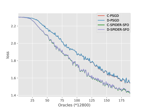
Figure 3: 3 is the experiments on CPU cluster with 8 nodes.

Hyper-parameters: For D-PSGD and C-PSGD, we use minibatch of size 128, that is, minibatch of size 16 for each node and tune the constant learning rate $\frac{\eta_{0}}{\sqrt{K/n}}$. For D-SPIDER-SFO and C-SPIDER-SFO, we set $S_{1}=256$, $S_{2}=16$, $q=16$ for each node and tune the learning rate for $\{0.1,0.05,0.01,0.005,0.001\}$.

References

• Assran et al. (2019) Assran, M.; Loizou, N.; Ballas, N.; and Rabbat, M. 2019. Stochastic gradient push for distributed deep learning. In Proceedings of the 36th International Conference on Machine Learning - Volume 97, 344–353.
• Dean et al. (2012) Dean, J.; Corrado, G.; Monga, R.; Chen, K.; Devin, M.; Mao, M.; aurelio Ranzato, M.; Senior, A.; Tucker, P.; Yang, K.; Le, Q. V.; and Ng, A. Y. 2012. Large scale distributed deep networks. In Advances in Neural Information Processing Systems 25, 1223–1231.
• Defazio, Bach, and Lacoste-Julien (2014) Defazio, A.; Bach, F.; and Lacoste-Julien, S. 2014. Saga: A fast incremental gradient method with support for non-strongly convex composite objectives. In Advances in Neural Information Processing Systems 27, 1646–1654.
• Dekel et al. (2012) Dekel, O.; Gilad-Bachrach, R.; Shamir, O.; and Xiao, L. 2012. Optimal distributed online prediction using mini-batches. Journal of Machine Learning Research 165–202.
• Devlin et al. (2019) Devlin, J.; Chang, M.-W.; Lee, K.; and Toutanova, K. 2019. Bert: Pre-training of deep bidirectional transformers for language understanding. In Proceedings of the 2019 Conference of the North American Chapter of the Association for Computational Linguistics: Human Language Technologies.
• Fang et al. (2018) Fang, C.; Li, C. J.; Lin, Z.; and Zhang, T. 2018. Spider: Near-optimal non-convex optimization via stochastic path-integrated differential estimator. In Advances in Neural Information Processing Systems 31, 689–699.
• Ghadimi and Lan (2013) Ghadimi, S., and Lan, G. 2013. Stochastic first- and zeroth-order methods for nonconvex stochastic programming. SIAM Journal on Optimization 2341–2368.
• He et al. (2015) He, K.; Zhang, X.; Ren, S.; and Sun, J. 2015. Deep residual learning for image recognition. In 2016 IEEE Conference on Computer Vision and Pattern Recognition (CVPR), 770–778.
• He et al. (2016) He, K.; Zhang, X.; Ren, S.; and Sun, J. 2016. Deep residual learning for image recognition. In Proceedings of the IEEE conference on computer vision and pattern recognition, 770–778.
• Huang et al. (2017) Huang, G.; Liu, Z.; Van Der Maaten, L.; and Weinberger, K. Q. 2017. Densely connected convolutional networks. In Proceedings of the IEEE conference on computer vision and pattern recognition.
• Jianmin et al. (2016) Jianmin, C.; Monga, R.; Bengio, S.; and Jozefowicz, R. 2016. Revisiting distributed synchronous sgd. In International Conference on Learning Representations Workshop Track.
• Johnson and Zhang (2013) Johnson, R., and Zhang, T. 2013. Accelerating stochastic gradient descent using predictive variance reduction. In Advances in Neural Information Processing Systems 26, 315–323.
• Krizhevsky and Hinton (2009) Krizhevsky, A., and Hinton, G. 2009. Learning multiple layers of features from tiny images. In Technical Report.
• Lecun et al. (1998) Lecun, Y.; Bottou, L.; Bengio, Y.; and Haffner, P. 1998. Gradient-based learning applied to document recognition. In Proceedings of the IEEE, 2278–2324.
• Lei et al. (2017) Lei, L.; Ju, C.; Chen, J.; and Jordan, M. I. 2017. Non-convex finite-sum optimization via scsg methods. In Advances in Neural Information Processing Systems 30, 2348–2358.
• Li et al. (2014) Li, M.; Andersen, D. G.; Park, J. W.; Smola, A. J.; Ahmed, A.; Josifovski, V.; Long, J.; Shekita, E. J.; and Su, B.-Y. 2014. Scaling distributed machine learning with the parameter server. In 11th USENIX Symposium on Operating Systems Design and Implementation (OSDI 14), 583–598.
• Lian et al. (2017) Lian, X.; Zhang, C.; Zhang, H.; Hsieh, C.-J.; Zhang, W.; and Liu, J. 2017. Can decentralized algorithms outperform centralized algorithms? a case study for decentralized parallel stochastic gradient descent. In Advances in Neural Information Processing Systems 30, 5330–5340.
• Mokhtari and Ribeiro (2016) Mokhtari, A., and Ribeiro, A. 2016. Dsa: Decentralized double stochastic averaging gradient algorithm. Journal of Machine Learning Research 2165–2199.
• Nedić and Ozdaglar (2009) Nedić, A., and Ozdaglar, A. 2009. Distributed subgradient methods for multi-agent optimization. IEEE Transactions on Automatic Control 48–61.
• Nguyen et al. (2017) Nguyen, L. M.; Liu, J.; Scheinberg, K.; and Takáč, M. 2017. Sarah: A novel method for machine learning problems using stochastic recursive gradient. In Proceedings of the 34th International Conference on Machine Learning, 2613–2621.
• Nguyen et al. (2019) Nguyen, L. M.; Dijk, M. v.; Phan, D. T.; Nguyen, P. H.; Weng, T.-W.; and Kalagnanam, J. R. 2019. Finite-sum smooth optimization with sarah. In arXiv preprint arXiv: 1901.07648.
• Reddi et al. (2016) Reddi, S. J.; Hefny, A.; Sra, S.; Póczós, B.; and Smola, A. J. 2016. Stochastic variance reduction for nonconvex optimization. In Proceedings of the 33rd International Conference on International Conference on Machine Learning - Volume 48, 314–323.
• Robbins and Monro (1951) Robbins, H., and Monro, S. 1951. A stochastic approximation method. The Annals of Mathematical Statistics 400–407.
• Roux, Schmidt, and Bach (2012) Roux, N. L.; Schmidt, M.; and Bach, F. R. 2012. A stochastic gradient method with an exponential convergence _rate for finite training sets. In Advances in Neural Information Processing Systems 25, 2663–2671.
• Scaman et al. (2018) Scaman, K.; Bach, F.; Bubeck, S.; Massoulié, L.; and Lee, Y. T. 2018. Optimal algorithms for non-smooth distributed optimization in networks. In Advances in Neural Information Processing Systems 31, 2740–2749.
• Shi et al. (2014) Shi, W.; Ling, Q.; Yuan, K.; Wu, G.; and Yin, W. 2014. On the linear convergence of the admm in decentralized consensus optimization. IEEE Transactions on Signal Processing 1750–1761.
• Tang et al. (2018) Tang, H.; Lian, X.; Yan, M.; Zhang, C.; and Liu, J. 2018. D2: Decentralized training over decentralized data. In Proceedings of the 35th International Conference on Machine Learning, 4848–4856.
• Vaswani et al. (2017) Vaswani, A.; Shazeer, N.; Parmar, N.; Uszkoreit, J.; Jones, L.; Gomez, A. N.; Kaiser, L. u.; and Polosukhin, I. 2017. Attention is all you need. In Advances in Neural Information Processing Systems 30, 5998–6008.
• Wei et al. (2015) Wei, S.; Qing, L.; Gang, W.; and Wotao, Y. 2015. Extra: An exact first-order algorithm for decentralized consensus optimization. SIAM Journal on Optimization 944–966.
• Yuan, Ling, and Yin (2016) Yuan, K.; Ling, Q.; and Yin, W. 2016. On the convergence of decentralized gradient descent. SIAM Journal on Optimization 26(3):1835–1854.
• Zhou, Xu, and Gu (2018) Zhou, D.; Xu, P.; and Gu, Q. 2018. Stochastic nested variance reduced gradient descent for nonconvex optimization. In Advances in Neural Information Processing Systems 31, 3921–3932.
• Zinkevich et al. (2010) Zinkevich, M.; Weimer, M.; Li, L.; and Smola, A. J. 2010. Parallelized stochastic gradient descent. In Advances in Neural Information Processing Systems 23, 2595–2603.