Optimal Multivariate Tuning with Neuron-Level and Population-Level Energy Constraints

Abstract

Optimality principles have been useful in explaining many aspects of biological systems. In the context of neural encoding in sensory areas, optimality is naturally formulated in a Bayesian setting, as neural tuning which minimizes mean decoding error. Many works optimize Fisher information, which approximates the Minimum Mean Square Error (MMSE) of the optimal decoder for long encoding time, but may be misleading for short encoding times. We study MMSE-optimal neural encoding of a multivariate stimulus by uniform populations of spiking neurons, under firing rate constraints for each neuron as well as for the entire population. We show that the population-level constraint is essential for the formulation of a well-posed problem having finite optimal tuning widths, and optimal tuning aligns with the principal components of the prior distribution. Numerical evaluation of the two-dimensional case shows that encoding only the dimension with higher variance is optimal for short encoding times. We also compare direct MMSE optimization to optimization of several proxies to MMSE, namely Fisher information, Maximum Likelihood estimation error, and the Bayesian Cramér-Rao bound. We find that optimization of these measures yield qualitatively misleading results regarding MMSE-optimal tuning and its dependence on encoding time and energy constraints.

1 Introduction

Optimality principles have been a useful tool in explaining many aspects of biological systems, including motor behavior [24], perception [14], and neural activity [3]. In the context of neural encoding in sensory areas, optimality is naturally formulated in a Bayesian setting, by specifying (i) a prior distribution of encoded stimuli; (ii) a performance criterion, such as mean decoding error or motor performance; (iii) optimization constraints, such as constraints on energy consumption. Empirically, neural encoding has been found to depend on the statistics of natural stimuli [3, 16], as well as to rapidly adapt to the statistics of recently presented stimuli [10, 2], indicating the importance of the prior distribution. Sensory adaptation also occurs following motor learning [8], suggesting the relevance of motor performance criteria, though the effect of motor learning on sensory perception is quite small. Since sensory encoding occurs in the context of an acting organism, an optimality criterion should ideally take the entire sensory-motor loop into account. However, to make the analysis tractable, most existing work has focused on task-independent measures of encoding performance, such as decoding error.

A natural optimality criterion for neural encoding is the Mean Square Error (MSE) of a subsequent optimal decoder, namely the Minimal Mean Square Error (MMSE) estimator. Many works optimize Fisher information, which serves as a proxy to the MSE (see [19] for a thorough review). Specifically, the Cramér-Rao Bound (CRB) states that the MSE of unbiased estimators is lower-bounded by the inverse of Fisher information. More importantly, under appropriate regularity conditions, the optimal MSE approaches the expected value of the CRB [25] in the asymptotic regime of low noise, corresponding to large decoding time or large population firing rate. Similar asymptotic relations can be derived between Fisher information and general $L_{p}$ estimation errors [26]. Fisher information of neural spiking activity is easy to compute analytically, at least in the case of static stimulus [9, section 3.3], and it can be used without characterizing the decoder. However, optimizing Fisher information may yield misleading qualitative results regarding the MSE-optimal encoding outside of the asymptotic regime of large decoding time [4, 27, 19]. Ideally, a model of biological encoding as optimal encoding should rely on biologically relevant optimality criteria such as decoding error, rather than a proxy to decoding error such as Fisher information. In particular, outside of the asymptotic regime, the CRB does not provide adequate justification for the use of Fisher information, since optimal decoding is typically biased, so the CRB does not apply to the optimal decoder.

Several previous works have attempted direct minimization of decoding MSE rather than Fisher information. [6] and two sequel articles [5, 7] analytically derive decoding MMSE for encoding a static scalar state uniformly distributed on $\left[0,1\right]$ by a single neuron, for a wide class of piecewise-power-law tuning functions. They find a phase transition between binary encoding, which is optimal for short coding times, and analog encoding, which is optimal for long coding times. In [27], an explicit expression for the MSE of the optimal Bayesian decoder is derived for a static state encoded by a uniform population of Gaussian neurons, and is used to characterize optimal tuning function width and its relation to coding time in the encoding of scalar stimuli. More recently, [26] studied $L_{p}$-based loss measures in the asymptotic regime using Fisher information, as well as numerically for the maximum a-posteriori estimator outside the asymptotic regime. [12] study the MSE of the ML estimator in the context of two-dimensional encoding of angles, used as a model for head direction encoding in bats. In [22, 23], a mean-field approximation is suggested to allow efficient evaluation of the MSE in a dynamic setting. We have previously used Assumed Density Filtering for the approximate evaluation of decoding MMSE for non-uniform populations and dynamic state in [15].

As far as we are aware, most previous works studying optimal neural encoding have paid little attention to the topic of energy constraints or other optimization constraints. Most commonly, optimization is performed over tuning width while keeping the maximal firing rate of each neuron fixed. In some cases (such as [26]), this is explicitly stated as a constraint on each neuron’s firing rate. However, even when the maximal firing rate of each neuron is constrained, tuning width affects the mean total firing rate – and therefore energy consumption – of the entire neural population. This issue has been addressed heuristically in [28] by studying Fisher information per spike as a measure of energy efficiency. However, the interpretation or significance of this ratio remains unclear. [4] have addressed this issue more systematically in the context of a univariate state taking values in a bounded interval, with a constraint on the mean firing rate as well as maximal firing rate of each neuron (see section 7 therein). MMSE was evaluated using Monte-Carlo methods, showing that imposing the energy constraint leads to narrower tuning. [13] also study optimal encoding with a parameterized population of neurons under a population rate constraint. However their analysis is based on optimization of Fisher information.

In this work, we focus on optimization of tuning widths in a multivariate setting, with constraints on the firing rate of each neuron as well as the entire population. To allow exact closed-form evaluation of decoding MMSE, we focus on uniform Gaussian encoding of a static stimulus. Optimization of tuning width involves a trade-off between population firing rate, which is maximized by wide tuning, and selectivity of individual neurons, which is maximized by narrow tuning [28, 11, 21]. Estimation MSE in a uniform Gaussian population is minimized for a finite nonzero width in the univariate case [27], and for infinitely wide tuning in the multivariate case, as shown in section 5. The addition of a constraint on the population firing rate gives rise to a finite-width solution in the multivariate case, in which both constraints are active. The constraint on the population firing rate may be interpreted as a sparsity constraint: for a fixed maximal firing rate per neuron, a smaller population rate constraint means less neurons may fire near their maximal rate for each stimulus. Optimal tuning depends on both energy constraints, as well as encoding time.

Applying the predictions of Bayesian MMSE-optimal tuning to explain experimentally observed coding is challenging. A substantial difficulty is the characterization of the relevant prior distribution that encoding is adapted to. In a few special cases, this prior may be derived from simple physical considerations (e.g. [16]), but such an approach is not usually applicable. Another difficulty is in the evaluation of decoding MMSE outside of the special case of Gaussian uniform coding, or conversely, identifying biological circumstances where the Gaussian uniform assumption is reasonable. Some biological implications of MMSE-optimality in the scalar case have been related to experimental results in [27]. In the multivariate case, there are fewer relevant experimental results where multivariate tuning is measured and the prior distribution and encoding time may be determined. Possibly relevant results are in the encoding of head direction in bats studied in [12]. However, it is not clear that the assumption of Gaussian uniform coding is justified in this case, as briefly discussed in section 5.2.

Main results: (i) Closed-form characterization of MMSE in multivariate uniform Gaussian encoding, as well as simple lower and upper bounds. (ii) A population-level constraint is essential to formulate a well-posed optimization problem in a multivariate setting, and optimal tuning depends on this constraint in a non-trivial way. (iii) MMSE-optimal multivariate Gaussian tuning functions are aligned with the principal components of the prior distribution and tuning is narrower in dimensions with larger prior variance. (iv) The trade-off between firing rate and neuron selectivity shifts with stimulus dimensionality, so that MSE-optimal multivariate encoding always involves maximizing population firing rate, in contrast to the univariate case. (v) Optimization of proxies to MMSE such as Fisher information or MSE of the Maximum Likelihood estimator yield qualitatively misleading results. (vi) In a two-dimensional setting, one-dimensional encoding is preferred for short decoding times, in contrast to previous predictions.

2 Setting and notation

2.1 Optimal encoding and decoding

We consider the problem of optimal encoding and decoding of a static external state, described by a random $m$-dimensional variable $X\in\mathbb{R}^{m}$. The state is observed through a population of sensory neurons over a time interval $[0,T]$. Given the state, neurons fire independently, with the $i$th neuron firing as a Poisson process with rate $\lambda^{\left(i\right)}\left(X\right)$. We assume the set $\{\lambda^{(i)}\}_{i=1}^{M}$ belongs to some parameterized family with parameter $\phi$, and denote the number of spikes from the $i$th neuron up to time $T$ by $N_{T}^{\left(i\right)}$ and the spike counts from all neurons by $\boldsymbol{N}_{T}\coloneqq(N_{T}^{\left(i\right)})_{i=1}^{M}$. In this context, encoding refers to the choice of functions $\lambda^{\left(i\right)}$, while decoding means estimating the state $X$ from the spike counts $\boldsymbol{N}_{T}$.

Given an estimator $\hat{X}=\hat{X}\left(\boldsymbol{N}_{T}\right)$, we define the Mean Square Error (MSE) as

$$\epsilon(\hat{X})\coloneqq\mathrm{tr}[(X-\hat{X})(X-\hat{X})^{\mathsf{T}}]$$ (1)

where $\mathrm{tr}$ is the trace operator. We seek an estimator (decoder) $\hat{X}$ and tuning parameters (encoder) $\phi$ that solve

$$\min_{\phi}\min_{\hat{X}}\mathrm{E}\left[\epsilon\right]=\min_{\phi}\mathrm{E}[\min_{\hat{X}}\mathrm{E}[\epsilon|\boldsymbol{N}_{T}]].$$

The inner minimization problem in this equation is solved by the MSE-optimal decoder, which is the posterior mean $\hat{X}=\mu_{T}\coloneqq\mathrm{E}\left[X|\boldsymbol{N}_{T}\right]$. We denote the error of this estimator by $\epsilon_{\mathrm{MMSE}}\coloneqq\epsilon\left(\mu_{T}\right)$ (for Minimum Mean Square Error). The outer minimization problem becomes $\min_{\phi}\mathbf{E}\left[\epsilon_{\mathrm{MMSE}}\right]$; its solution is the optimal encoder.

We also compare MSE-optimal encoding and decoding to three alternative performance criteria.

• Maximization of Fisher information,

• Minimization of the Bayesian Cramér-Rao bound,

• Optimization of MSE (1) for the Maximum Likelihood (ML) estimator.

These performance criteria are defined and discussed in section 4.

2.2 Uniform-Gaussian coding

For mathematical tractability, we focus on the case of homogeneous Gaussian tuning, which is a special case of that studied in [15]: the firing rate of the $i$th neuron in response to state $x$ is given by

$$\lambda^{i}\left(x\right)=h_{\mathrm{d}}\exp\left(-\frac{1}{2}\left\|x-\theta^{\left(i\right)}\right\|_{R}^{2}\right),$$ (2)

where $\theta^{\left(i\right)}\in\mathbb{R}^{m}$ is the $i$th neuron’s preferred stimulus, $h_{\mathrm{d}}\in\mathbb{R}_{+}$ is each neuron’s maximal expected firing rate, $R\in\mathbb{R}^{m\times m}$ is a symmetric positive-definite matrix, and the notation $\left\|y\right\|_{M}^{2}$ denotes $y^{T}My$. The distribution of the external state $X$ is assumed to be Gaussian,

$$X\sim\mathcal{N}\left(\mu_{0},\Sigma_{0}\right).$$ (3)

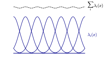
(a) uniform coding

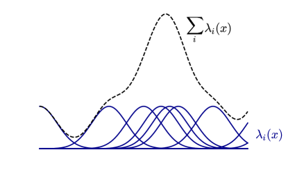
(b) non-uniform coding

Figure 1: The uniform coding property, $\Sigma_{i}\lambda^{i}\left(x\right)=\mathrm{const}$, holds approximately in homogeneous populations with tuning function centers located on a dense uniform grid, as demonstrated in (a) in a 1-dimensional case. (b) illustrates non-uniform coding. Reprinted from [15].

We assume preferred stimuli $\theta^{\left(i\right)}$ are spaced uniformly on an infinite grid with spacing $\Delta\theta$, so there is one neuron for each preferred stimulus of the form $\left(\alpha_{1},\ldots,\alpha_{m}\right)^{\mathsf{T}}\Delta\theta$ where each $\alpha_{i}$ is an integer. When $\Delta\theta$ is reasonably small relative to the eigenvalues of $R^{-1/2}$, the total firing rate $\sum_{i}\lambda\left(x\right)$ is approximately independent of $x$, a property that we refer to as uniform coding (see Figure 1 and discussion in [15]). For small $\Delta\theta$, we may approximate the neural populations by an infinite continuous population where the preferred stimulus $\theta$ may take any value in $\mathbb{R}^{m}$ (see Figure 2). In this continuous population model, each spike is characterized by the preferred stimulus of the firing neuron – which is a continuous variable – rather than by the neuron’s index. Thus, the firing pattern is described by a marked point process (MPP) $N$, which is a random sequence of pairs $\left(t_{k},\theta_{k}\right)$, where $t_{k}\in[0,\infty)$ is the time of the $k$th spike and $\theta_{k}\in\mathbb{R}^{m}$ its mark, which is the preferred stimulus of the spiking neuron. A marked point process is characterized by the rate of points with marks in each (measurable) subset $\Theta\subseteq\mathbb{R}^{m}$, which in the discrete population model (2) is given by

$$\lambda\left(x;\Theta\right) =\sum_{i:\theta_{i}\in\Theta}\lambda^{i}\left(x\right)=h_{\mathrm{d}}\sum_{i:\theta^{\left(i\right)}\in\Theta}\exp\left(-\frac{1}{2}\left\|x-\theta^{\left(i\right)}\right\|_{R}^{2}\right)$$

$$\approx\frac{h_{\mathrm{d}}}{\Delta\theta^{m}}\int_{\Theta}\exp\left(-\frac{1}{2}\left\|x-\theta\right\|_{R}^{2}\right)d\theta$$

The approximate equality in the second line is exact in the limit $\Delta\theta\to 0$ with $h\coloneqq h_{\mathrm{d}}\Delta\theta^{-m}$ fixed. Accordingly, in the continuous population model we take the MPP $N$ to have the space-time density

$$\lambda\left(x;\theta\right)\coloneqq h\exp\left(-\frac{1}{2}\left\|x-\theta\right\|_{R}^{2}\right),$$ (4)

meaning that the rate of points with marks in $\Theta\subseteq\mathbb{R}^{m}$ is $\int_{\Theta}\lambda\left(x;\theta\right)d\theta$. In the continuous population model, we use the notation $\boldsymbol{N}_{t}$ to refer to the sequence of spike times and marks up to time $t$, that is $\boldsymbol{N}_{t}\coloneqq\left(t_{k},\theta_{k}\right)_{k=1}^{N_{t}}$. The probability density of $\boldsymbol{N}_{T}$ given $X=x$ is

$$p\left(\left(t_{k},\theta_{k}\right)_{k=1}^{N_{T}}|X=x\right) =e^{-rT}\prod_{k=1}^{N_{T}}\lambda\left(x;\theta_{k}\right)\quad\left(t_{1}<\cdots<t_{N_{T}}\right)$$ (5)

where

$$r\coloneqq\int_{\mathbb{R}^{m}}\lambda\left(x;\theta\right)d\theta=h\sqrt{\frac{\left(2\pi\right)^{m}}{\det R}}$$ (6)

is the total population rate. The likelihood (5) does not depend on spike times $t_{k}$, only on preferred stimuli $\theta_{k}$, so the sequence of preferred stimuli comprises a sufficient statistic for the estimation of $X$.

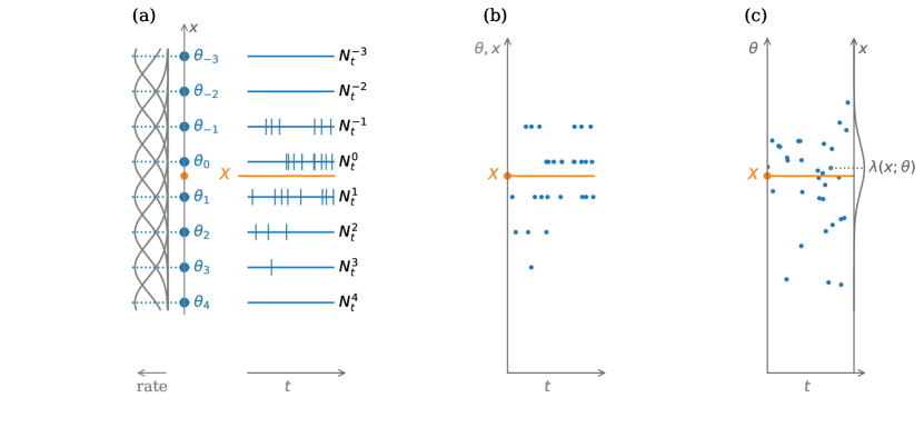
Figure 2: Discrete and continuous population models. (a) A discrete population of neurons with preferred stimuli $\theta_{i}$ on a uniform grid. The tuning functions are depicted on the left. The spiking pattern of each neuron in response to the stimulus $X$ (orange line) is represented by a separate point processes $N_{t}^{i}$ (blue vertical ticks). (b) A representation of the same neural response as a single marked point process. Each blue dot represents a spike with the vertical location representing its mark $\theta$. (c) A continuous population model approximating the statistics of the same population. The approximation would be better for larger populations. The tuning function corresponding to one of the spikes is depicted on the right. Adapted from [15].

2.3 Energy constraints

Clearly, the solution to the optimal encoding problem depends crucially on the family of encodings over which optimization is performed. In particular, if optimization is entirely unconstrained, the MMSE can always be decreased by scaling the maximal rate-density $h$ in (4) by some constant $k>1$, thereby uniformly increasing all firing rates. The unconstrained problem is therefore mathematically ill-posed. However, firing rates of real neurons cannot grow without bound. Although optimization constraints are rarely discussed explicitly, all works mentioned above – apart from [4] – implicitly constrain the neural population in the same way: by fixing the maximal firing rate $h$ (or $h_{\mathrm{d}}$ in a discrete model) across all neurons and optimizing only preferred stimuli and/or tuning widths. Note that the continuous model approximates a discrete population with $h=h_{\mathrm{d}}/\Delta\theta^{m}$, so that constraining the rate-density $h$ translates to a constraint on maximal firing rates $h_{\mathrm{d}}$ of individual neurons.

We propose that in addition to a constraint on maximal rate-density $h$, the expected total firing rate of the population should also be constrained when formulating the optimal encoding problem. Biologically, such a constraint corresponds to a constraint on the expected rate of energy use by the neural population [28]. As demonstrated below, this constraint may be crucial to make the problem mathematically well-posed, even in the presence of a neuron-level constraint on $h$. The energy-constrained problem takes the form

$$\min_{h,R}\; \epsilon_{\mathrm{MMSE}}=\epsilon\left(\mu_{T}\right)=\mathbf{E}\left[\mathrm{\mathrm{tr}}[(X-\mu_{T})(X-\mu_{T})^{\mathsf{T}}]\right]$$

$$\mathrm{s.t.}\; h\leq\bar{h}$$

$$r=h\sqrt{\frac{\left(2\pi\right)^{m}}{\det R}}\leq\bar{r}$$ (7)

where $\mu_{T}\coloneqq\mathrm{E}\left[X|\boldsymbol{N}_{T}\right]$.

The population firing rate constraint may also be interpreted as a sparsity constraint: for a fixed neuron-level rate constraint $\bar{h}$, higher population rate $r$ is related to wider tuning resulting in more neurons firing in response to the same stimulus. Low values of the population constraint $\bar{r}$ thus enforce sparse coding, where only a few neurons fire in response to each stimulus value.

3 Closed-form computation of estimation error

3.1 General multivariate case

The posterior distribution for the model (3)-(5) is Gaussian,

$$X|\boldsymbol{N}_{T}\sim\mathcal{N}\left(\mu_{T},\Sigma_{T}\right)$$

where

$$\mu_{T} =\Sigma_{T}\left(\Sigma_{0}^{-1}\mu_{0}+R\sum_{i=1}^{N_{T}}\theta_{i}\right),$$

$$\Sigma_{T} =\left(\Sigma_{0}^{-1}+N_{T}R\right)^{-1}.$$ (8)

This result is a special case of [20, Theorem 1]. The estimation MMSE is therefore

$$\epsilon_{\mathrm{MMSE}} =\mathrm{\mathrm{tr}}\mathbf{E}\left[(X-\mu_{T})(X-\mu_{T})^{\mathsf{T}}\right]=\mathrm{\mathrm{tr}}\mathbf{E}\mathbf{E}\left[(X-\mu_{T})(X-\mu_{T})^{\mathsf{T}}|\boldsymbol{N}_{T}\right]$$

$$=\mathrm{tr}\,\mathbf{E}[\Sigma_{T}]=\mathrm{tr}\,\mathbf{E}\left[\left(\Sigma_{0}^{-1}+N_{T}R\right)^{-1}\right],$$

where

$$N_{T}\sim\mathrm{Pois}\left(\sqrt{\frac{\left(2\pi\right)^{m}}{\det R}}hT\right)$$

(see (6)), yielding the closed-form expression

$$\epsilon_{\mathrm{MMSE}}=\exp\left(-\sqrt{\frac{\left(2\pi\right)^{m}}{\det R}}hT\right)\sum_{k=0}^{\infty}\frac{1}{k!}\left(\sqrt{\frac{\left(2\pi\right)^{m}}{\det R}}hT\right)^{k}\mathrm{tr}\left((kR+\Sigma_{0}^{-1})^{-1}\right).$$ (9)

3.2 Diagonal tuning

An important special case of (9) is where the prior variance $\Sigma_{0}$ and tuning precision $R$ are both diagonal, $m=n$, and $H=I$, with

$$\Sigma_{0} =\mathrm{diag}\left(\sigma_{0,1}^{2},\sigma_{0,2}^{2},\ldots\sigma_{0,m}^{2}\right),$$ (10)

$$R =\mathrm{diag}\left(\alpha_{1}^{-2},\ldots\alpha_{m}^{-2}\right).$$ (11)

In section 5 we show that the general optimization problem (7), (9) may be reduced to this case, so there is no loss of generality here. In this diagonal case, the total population rate is

$$r=\left(2\pi\right)^{m/2}h\prod_{i}\alpha_{i},$$ (12)

and (9) reads

$$\epsilon_{\mathrm{MMSE}} =\exp\left(-h^{\prime}T\prod_{j}\alpha_{j}\right)\sum_{k=0}^{\infty}\frac{(h^{\prime}T\prod_{j}\alpha_{j})^{k}}{k!}\sum_{i=1}^{m}\frac{1}{\sigma_{0,i}^{-2}+k\alpha_{i}^{-2}},$$

$$=\sum_{i=1}^{m}\sigma_{0,i}^{2}\,q\left(\frac{\alpha_{i}^{2}}{\sigma_{0,i}^{2}},h^{\prime}T\prod_{j}\alpha_{j}\right),$$ (13)

where $h^{\prime}\coloneqq\left(2\pi\right)^{m/2}h$ and we define, for $s,r>0$,

$$q\left(s,r\right)\coloneqq se^{-r}\sum_{k=0}^{\infty}\frac{r^{k}}{k!\left(s+k\right)}=M\left(1,s+1,-r\right),$$ (14)

where $M$ is Kummer’s confluent hypergeometric function [1]. This result for the diagonal case has previously appeared in [27].

In particular, the estimation error in the $i$th direction is given by the $i$th summand in (13), namely $\sigma_{0,i}^{2}\,q(\alpha_{i}^{2}/\sigma_{0,i}^{2},h^{\prime}T\prod_{j}\alpha_{j})$. The function $q$ takes values in the interval $\left[0,1\right]$, so this factor represents the reduction of prior variance due to observation of the spiking activity. More specifically, $q\left(s,r\right)$ satisfies the bounds

$$\left(1+\frac{r}{s}\right)^{-1}\leq q\left(s,r\right)\leq\left(1+\frac{r}{s+1}\right)^{-1}.$$ (15)

The lower bound is obtained by applying Jensen’s inequality to the convex function $k\mapsto s/\left(s+k\right)$ in (14). The upper bound may be obtained from [17, Theorem 15] by taking the limit $a\to 1$ with $c=a+1$ in equation (5.4) therein. This yields the following bounds for the MMSE

$$\sum_{i=1}^{m}\left(\frac{1}{\sigma_{0,i}^{2}}+\frac{h^{\prime}T\prod_{j}\alpha_{j}}{\alpha_{i}^{2}}\right)^{-1}\leq\epsilon_{\mathrm{MMSE}}\leq\sum_{i=1}^{m}\left(\frac{1}{\sigma_{0,i}^{2}}+\frac{h^{\prime}T\prod_{j}\alpha_{j}}{\alpha_{i}^{2}+\sigma_{0,i}^{2}}\right)^{-1}$$ (16)

We also use the following property of the function $q$, which is proved by a direct calculation of the derivative, as outlined in appendix A.2.

Claim 1.

For any $c_{1},c_{2}\in\mathbb{R}_{+}$ and $m\geq 2$ , $q\left(c_{1}\alpha^{2},c_{2}\alpha^{m}\right)$ is a decreasing function of $\alpha\in(0,\infty)$.

4 Alternate performance criteria

4.1 Motivation

Estimation MMSE is generally difficult to evaluate, except in specific cases where the posterior distribution can be described analytically, such as the model considered in the present work. This motivates the optimization of more tractable approximations or bounds to the MMSE. Of these, the most commonly used is Fisher information, which is related to the MMSE through the Cramér-Rao bound (CRB) and the Bayesian Cramér-Rao bound (BCRB) [25, 27]. Another class of proxies is the MSE of suboptimal estimators such as the maximum likelihood estimator (as used, e.g., in [12]) or the maximum a-posteriori estimator (as used, e.g., in [26]). In section 5.2 we compare the minimization of MMSE in the model (3)-(5) to optimization of several other performance criteria, in order to evaluate their applicability as proxies to MMSE minimization.

4.2 MSE of the maximum likelihood estimator

Previous works such as [12] use the MSE of the Maximum Likelihood (ML) estimator as a performance criterion. The ML estimator may be easier to compute, especially for non-uniform coding. However, it is not the optimal estimator, so optimization of encoding for subsequent ML decoding does not optimize decoding error of the encoder-decoder system. Using the ML estimator may be justified for long decoding time or large firing rates, where the effect of the prior on the posterior distribution becomes negligible. However, in this regime, Fisher information may also be useful and easier to evaluate. In section 5.2, we investigate the minimization of ML estimation error in our model to assess whether it resembles minimization of MMSE for short decoding times, at least qualitatively.

There is a difficulty with the definition of the ML estimator in the uniform-Gaussian model: when there are no spikes, the likelihood (5) is $\mathrm{P}\left(N_{T}=0|X=x\right)=e^{-rT}$, which is independent of $x$, so the ML estimator is undefined. This is a direct consequence of the uniform coding property, as the population rate $r$ is independent of $x$. We therefore use a modified ML estimator, which equals the prior $\mu_{0}$ in the case where there are no spikes,

$$\hat{X}_{t}^{\mathrm{ML}}=\begin{cases}\frac{1}{N_{t}}\sum_{i=1}^{N_{t}}\theta_{i}&N_{t}>0,\\ \mu_{0}&N_{t}=0,\end{cases}$$ (17)

where $\theta_{i}$ is the preferred stimulus of the neuron firing the $i$th spike. This modified ML estimator may be obtained from the MMSE estimator in the limit $\Sigma_{0}^{-1}\to 0$.

The MSE of this estimator can be written in closed form (see appendix (A.1)) as

$$\epsilon\left(\hat{X}_{T}^{\mathrm{ML}}\right) =e^{-rT}\left[\left(\sum_{k=1}^{\infty}\frac{\left(rT\right)^{k}}{k!\,k}\right)\sum_{i=1}^{m}\alpha_{i}^{2}+\sum_{i=1}^{m}\sigma_{i}^{2}\right],$$ (18)

where the second term is related to the case where there are no spikes. For fixed $h$ and $r=\left(2\pi\right)^{m/2}h\prod_{i}\alpha_{i}$, ML MSE (18) is minimized by minimizing $\sum_{i}\alpha_{i}^{2}$, yielding the symmetric solution

$$\alpha_{1}=\alpha_{2}=\cdots=\alpha_{m}=\left(2\pi\right)^{-1/2}\left(\frac{r}{h}\right)^{1/m}.$$ (19)

4.3 Fisher information / Cramér-Rao bound

The CRB is a lower bound on the MSE of an unbiased estimator for a non-random parameter. In a Bayesian setting, it may be used to bound the conditional MSE of an unbiased estimator $\hat{X}$ conditioned on the random state $X$. Under suitable regularity conditions, the bound reads [25]

$$S\left(\hat{X}|X\right)\coloneqq\mathbf{E}\left[\left.\left(\hat{X}-X\right)\left(\hat{X}-X\right)^{\mathsf{T}}\right|X\right]\succeq J\left(X\right)^{-1},$$

where the relation $\succeq$ means that the difference $S\left(\hat{X}|X\right)-J\left(X\right)^{-1}$ is positive semidefinite, and $J\left(X\right)$ is the Fisher information matrix, related to the likelihood function $p_{Y|X}$ as

$$J_{ij}\left(x\right)\coloneqq-\mathbf{E}\left[\left.\frac{\partial^{2}\log p_{Y|X}\left(Y|x\right)}{\partial x_{i}\partial x_{j}}\right|X=x\right].$$

As noted in the introduction, use of the Fisher information as a performance criterion may be justified asymptotically, for large decoding times or large population total firing rate. In this limit, the optimal MSE approaches the CRB under mild conditions (see discussion in [4]). Outside of the asymptotic regime, minimization of the CRB may differ from MSE minimization since optimal estimators are typically biased, and even among unbiased estimators, the bound may not be attainable. Note that the continuous population model we study here is generally not within this asymptotic regime despite having infinitely many neurons, since the total firing rate is kept finite.

In the case of a scalar state $x$ and a finite neural population with tuning functions $\lambda_{k}$, Fisher information for the estimation of $x$ from the spike counts over time interval $T$ is given by [9]

$$J\left(x\right)=T\sum_{k}\frac{\left(\lambda^{\prime}_{k}\left(x\right)\right)^{2}}{\lambda_{k}\left(x\right)}.$$

Similarly, in the continuous population model with multivariate state, (4)-(5), the Fisher information matrix takes the form

$$J\left(x\right)=T\int\frac{\nabla_{x}\lambda\left(x;\theta\right)\nabla_{x}\lambda\left(x;\theta\right)^{\mathsf{T}}}{\lambda\left(x;\theta\right)}d\theta=h^{\prime}T\left|R\right|^{-1/2}R=rTR,$$ (20)

(see derivation in appendix, section A.3) and the MSE of any unbiased estimator is therefore bounded by

$$\epsilon\left(\hat{X}\right)=\mathbf{E}\,\mathrm{tr}\,S\left(\hat{X}|X\right)\geq\mathbf{E}\,\mathrm{tr}\left(J^{-1}\right)=\frac{1}{rT}\mathrm{tr}\left(R^{-1}\right)=\frac{\sum_{i}\alpha_{i}^{2}}{rT}=\frac{\sum_{i}\alpha_{i}^{2}}{h^{\prime}T\prod_{i}\alpha_{i}},$$ (21)

For fixed population rate $r$, this bound is minimized by the same tuning widths (19) as the MSE of the modified ML estimator (17). This results in the minimal population inverse Fisher information

$$\min\mathbf{E}\,\mathrm{tr}\left(J^{-1}\right)=\frac{m}{h^{\prime}T}\alpha^{2-m},$$ (22)

where the tuning width $\alpha$ is related to rate density $h$ and population rate $r$ through (19). Equation (22) demonstrates that in the absence of population rate constraint, the Fisher-optimal widths are zero in the univariate case $m=1$ and infinite for $m>2$, whereas in the two-dimensional case $m=2$, population Fisher information is independent of tuning width. This is a special case of a result from [28] which applies more generally to radially symmetric tuning. This preference for wide tuning in higher dimensions may be explained by the fact that encoding accuracy in each dimension benefits from wide tuning in other dimensions, due to an increase in population firing rate, as noted in [11] (see Figure 1 therein).

Note that the modified ML estimator (17) is not an unbiased estimator; its bias is $\left(\mu_{0}-X\right)P\left\{N_{t}=0|X\right\}=\left(\mu_{0}-X\right)e^{-rT}$. Therefore its MSE is not bounded by (21), though we may expect it to satisfy the bound when $P\left(N_{t}=0\right)$ is small.

4.4 Bayesian Cramér-Rao bound

The Bayesian Cramér-Rao Bound (BCRB) is a lower bound on estimation error in a Bayesian setting. Under suitable regularity conditions, the MSE of any estimator $\hat{X}$ is bounded as [25]

$$S\left(\hat{X}\right)\coloneqq\mathbf{E}\left[\left(\hat{X}-X\right)\left(\hat{X}-X\right)^{\mathsf{T}}\right]\succeq\left(\mathbf{E}\left[J\left(X\right)\right]+J_{\mathrm{P}}\right)^{-1},$$ (23)

where $J\left(X\right)$ is the Fisher information matrix and $J_{\mathrm{P}}$ is the Bayesian information matrix, related to the prior density $p_{X}$ by

$$\left[J_{\mathrm{P}}\right]_{ij}=-\mathbf{E}\left[\frac{\partial^{2}\log p_{X}\left(X\right)}{\partial x_{i}\partial x_{j}}\right].$$

The BCRB is not restricted to unbiased estimators and is therefore applicable as a bound on optimal estimation error in a Bayesian setting outside of the asymptotic regime of large decoding time or population firing rate. On the other hand, unlike the CRB, the BCRB is generally not attained asymptotically: in the limit of infinite decoding time, the MMSE approaches the expected value of the CRB, $\mathbf{E}[J\left(X\right)^{-1}]$, whereas the BCRB approaches $\mathbf{E}\left[J\left(X\right)\right]^{-1}$, which generally underestimates the asymptotic MMSE [25]. In other words, the ratio $\mathrm{MMSE}/\mathrm{BCRB}$ may approach a value strictly larger 1 in the infinite decoding time limit. As evident from (23), in the univariate case minimization of the BCRB is equivalent to maximization of Fisher information. This equivalence does not hold in higher dimensions, as demonstrated below in the 2-dimensional case.

In the continuous population model (3)-(5), the BCRB reads

$$S\left(\hat{X}\right)\succeq\left(h^{\prime}T\left|R\right|^{-1/2}R+\Sigma_{0}^{-1}\right)^{-1},$$

where we have used (20). Applying the bound to the MMSE estimator in the diagonal case,

$$\epsilon_{\mathrm{MMSE}}=\mathrm{tr}\,S\left(\hat{X}_{\mathrm{MMSE}}\right) \geq\sum_{i=1}^{m}\left(\sigma_{0,i}^{-2}+h^{\prime}T\left(\prod_{j}\alpha_{j}\right)\alpha_{i}^{-2}\right)^{-1}$$ (24)

$$=\sum_{i=1}^{m}\left(\sigma_{0,i}^{-2}+rT\alpha_{i}^{-2}\right)^{-1},$$ (25)

which is the same lower bound as in (16).

5 Optimal encoding

5.1 MMSE-optimal multivariate tuning

Substituting (9) into (7), we obtain the optimization problem

$$\min_{R,h^{\prime}}\quad \exp\left(-\frac{h^{\prime}T}{\sqrt{\det R}}\right)\sum_{k=0}^{\infty}\frac{1}{k!}\left(\frac{h^{\prime}T}{\sqrt{\det R}}\right)^{k}\mathrm{tr}\left((kR+\Sigma_{0}^{-1})^{-1}\right),$$ (26)

$$\mathrm{s.t.}\quad h^{\prime}\leq\bar{h}^{\prime},$$

$$\frac{h^{\prime}}{\sqrt{\det R}}\leq\bar{r},$$

Denote the spectral decomposition for the prior variance by $\Sigma_{0}\coloneqq V_{0}\Lambda_{0}V_{0}^{\mathsf{T}}$ with $\Lambda_{0}$ diagonal and $V_{0}$ orthogonal. The principal components of the random vector $X$ are $\tilde{X}\coloneqq V_{0}^{\mathsf{T}}X$, which has the diagonal prior variance $\mathbf{E}[\tilde{X}\tilde{X}^{\mathsf{T}}]=\Lambda_{0}$. The population rate-density (4) may be written in terms of the principal components as

$$\tilde{\lambda}\left(\tilde{x};\tilde{\theta}\right) \coloneqq h\exp\left(-\frac{1}{2}\left\|\tilde{x}-\tilde{\theta}\right\|_{\tilde{R}}^{2}\right)=\lambda\left(x;\theta\right),$$ (27)

where

$$\tilde{R} =V_{0}^{\mathsf{T}}RV_{0},$$

$$\tilde{x} =V_{0}^{\mathsf{T}}x,\quad\tilde{\theta}=V_{0}^{\mathsf{T}}\theta.$$

The optimization problem may be reformulated as minimization of decoding MMSE for the principal component vector $\tilde{X}$, since neither the objective function nor the constraints in (7) are affected by the orthogonal transformation $V_{0}$. Specifically, the decoding MMSE of $\tilde{X}$ is $\mathrm{tr}[V_{0}E_{X}V_{0}^{\mathsf{T}}]=\mathrm{tr}\left[V^{\mathsf{T}}_{0}V_{0}E_{X}\right]=E_{X}$ where $E_{X}\coloneqq\mathbf{E}[(X-\hat{X})(X-\hat{X})]^{\mathsf{T}}$ is the decoding MMSE of $X$; and the optimization constraints depend on $R$ only through $\det R=\det\tilde{R}$. We therefore assume from here on, without loss of generality, that $\Sigma_{0}$ is diagonal with decreasing elements,

$$\Sigma_{0} =\mathrm{diag}\left(\sigma_{0,1}^{2},\sigma_{0,2}^{2},\ldots\sigma_{0,m}^{2}\right),$$

$$\sigma_{0,1}^{2}\geq\sigma_{0,2}^{2}\geq\cdots\geq\sigma_{0,m}^{2}.$$

The problem is further reduced by writing the spectral decomposition $R=U\Lambda U^{\mathsf{T}}$ and $Q\coloneqq\Sigma_{0}^{-1}$, and using the following claim, proved in appendix A.2

Claim 2.

Let $\Lambda,Q$ be diagonal positive definite matrices, $\Lambda=\mathrm{diag}\left(\lambda_{i}\right),Q=\mathrm{diag}\left(q_{i}\right)$ where $0<\lambda_{1}\leq\lambda_{2}\leq\cdots\lambda_{n}$ and $0<q_{1}\leq q_{2}\leq\cdots\leq q_{n}$. Then the constrained minimization problem

$$\min_{U}\; \mathrm{tr}\left[\left(Q+U\Lambda U^{\mathsf{T}}\right)^{-1}\right]$$

$$\mathrm{s.t.}\; UU^{\mathsf{T}}=I$$

is solved by $U$ anti-diagonal $u_{ij}=\delta_{i,\left(n+1-j\right)}$.

This shows that for a fixed choice of eigenvalues for $R$, each term in (26) is minimized by the same choice of eigenvectors, namely antidiagonal $u_{ij}=\delta_{i,\left(n+1-j\right)}$, which makes $R$ a diagonal matrix with elements sorted in decreasing order. Therefore this $U$ also minimizes the sum in (26) for fixed eigenvalues. Since the constraints depend on $R$ only through its eigenvalues, the optimal solution is of the same form, and in particular $R$ is diagonal and tuning is narrower (larger eigenvalues of $R$) in directions with larger prior variance (smaller eigenvalues of $Q$). In the more general case where $X$ has correlated components, applying this result to the principal components $\tilde{X}$ as outlined above shows that optimal tuning is aligned to principal components, $R=V_{0}\tilde{R}V_{0}^{\mathsf{T}}$ where $\tilde{R}$ is diagonal and principal components are in the columns of $V_{0}$.

We have reduced the problem to the case of diagonal prior $\Sigma_{0}=\mathrm{diag}\left(\sigma_{0,1}^{2},\sigma_{0,2}^{2},\ldots\sigma_{0,m}^{2}\right)$ and tuning $R=\mathrm{diag}\left(\alpha_{1}^{-2},\ldots\alpha_{m}^{-2}\right)$. Substituting (13) into (7), we obtain the optimization problem

$$\min_{\boldsymbol{\alpha},h^{\prime}}\quad \sum_{i=1}^{m}\sigma_{0,i}^{2}q\left(\frac{\alpha_{i}^{2}}{\sigma_{0,i}^{2}},h^{\prime}T\prod_{j}\alpha_{j}\right),$$

$$\mathrm{s.t.}\quad h^{\prime}\leq\bar{h}^{\prime},$$

$$h^{\prime}\prod_{i}\alpha_{i}\leq\bar{r},$$

where $\boldsymbol{\alpha}=\left(\alpha_{1},\ldots\alpha_{m}\right),h^{\prime}=\left(2\pi\right)^{m/2}h$, $\bar{h}^{\prime}=\left(2\pi\right)^{m/2}\bar{h}$, and $q$ is given by (14). The problem may be re-parameterized in terms of $\boldsymbol{\alpha}$ and $r$, where $r=h^{\prime}\prod\alpha_{i}$ is the total population rate,

$$\min_{\boldsymbol{\alpha},r}\quad \sum_{i=1}^{m}\sigma_{0,i}^{2}q\left(\frac{\alpha_{i}^{2}}{\sigma_{0,i}^{2}},rT\right),$$ (28)

$$\mathrm{s.t.}\quad r\leq\bar{h}^{\prime}\prod_{i}\alpha_{i},$$

$$r\leq\bar{r}.$$

Note that $q\left(s,r\right)$ is increasing in $s$ for fixed $r$, as evident from (14). Therefore, for fixed $r$, the objective (28) is an increasing function of each $\alpha_{i}$, so the solution satisfies the first constraint with equality, $\prod_{i}\alpha_{i}=r/\bar{h}^{\prime}$, or equivalently $h^{\prime}=\bar{h}^{\prime}$, and the problem reduces to

$$\min_{\boldsymbol{\alpha}\in\mathbb{R}^{m}}\quad \sum_{i=1}^{m}\sigma_{0,i}^{2}q\left(\frac{\alpha_{i}^{2}}{\sigma_{0,i}^{2}},\bar{h}^{\prime}T\prod_{j}\alpha_{j}\right)$$ (29)

$$\mathrm{s.t.}\quad \prod_{i}\alpha_{i}\leq\frac{\bar{r}}{\bar{h}^{\prime}}.$$ (30)

The unconstrained version of this problem in the scalar case $m=1$ has been studied in [27], where it was shown that optimal tuning width decreases with encoding time and increases with prior variance, consistent with experimental results. In this scalar case, the addition of the constraint (30) modifies the solution in a simple way by fixing the tuning width $\alpha$ to its constraint $\bar{r}/\bar{h}^{\prime}$ when the unconstrained problem is solved by a larger value of $\alpha$.

Using claim 1, for $m\geq 2$, any scaling of all $\alpha_{i}$ by the same factor $>1$ would reduce the MMSE, so the remaining constraint is also satisfied with equality, yielding the problem

$$\min_{\boldsymbol{\alpha}\in\mathbb{R}^{m}}\quad \sum_{i=1}^{m}\sigma_{0,i}^{2}q\left(\frac{\alpha_{i}^{2}}{\sigma_{0,i}^{2}},\bar{r}T\right)\quad\left(m\geq 2\right)$$ (31)

$$\mathrm{s.t.}\quad \prod_{i}\alpha_{i}=\frac{\bar{r}}{\bar{h}^{\prime}}$$ (32)

Similarly, claim 1 implies that the unconstrained version of (29) has no finite solution for $m\geq 2$, as the minimal error is attained in the limit of infinitely wide tuning. Equivalently, the minimization of the MMSE with neuron-level constraint only and no population-level constraint is solved in the limit of infinitely wide tuning, demonstrating the importance of the population-level constraint in this model.

To understand this difference between the scalar case $m=1$ and vector case $m\geq 2$, note that broadening the tuning has two effects: (i) increasing the spike rate, and (ii) making each spike less informative. Specifically, the population spike rate is proportional to the product of all tuning widths, $r=h^{\prime}\prod_{i}\alpha_{i}$, so that wider tuning yields higher population rates. On the other hand, (8) in the diagonal case reads

$$\sigma_{t,i}^{-2}=\sigma_{0,i}^{-2}+N_{t}\alpha_{i}^{-2},$$

where $\sigma_{t,i}^{-2}$ is the posterior precision (inverse of variance) of $X_{i}$ conditioned on $\boldsymbol{N}_{t}$, so that narrower tuning yields more informative spikes. In the scalar case, $m=1$, the trade-off between these two effects leads to a finite optimal tuning width. In higher dimensions, $m\geq 2$, all tuning widths contribute to the firing rate, but the effect of each spike on the posterior precision in dimension $i$ depends only on $\alpha_{i}$. Thus, optimizing the tuning width $\alpha_{i}$ involves a trade-off for the posterior variance $\sigma_{t,i}^{2}$ of $X_{i}$, but affects $\sigma_{t,j}^{2}$ for any other direction $j\neq i$ monotonically: increasing the tuning width $\alpha_{i}$ can only decrease $\sigma_{t,j}^{2}$ for $j\neq i$, through its effect on the population rate. This shifts the trade-off towards wider tuning in higher dimensions.

This effect can be seen more explicitly by approximating the objective (29) using the bounds (15) as

$$\epsilon^{\prime}\left(\boldsymbol{\alpha};0\right)\leq\mathrm{MMSE}\leq\epsilon^{\prime}\left(\boldsymbol{\alpha};1\right)$$

where

$$\epsilon^{\prime}\left(\boldsymbol{\alpha};\beta\right)\coloneqq\sum_{i=1}^{m}\left(\sigma_{0,i}^{-2}+\frac{\bar{h}^{\prime}T\prod_{j}\alpha_{j}}{\alpha_{i}^{2}+\beta\sigma_{0,i}^{2}}\right)^{-1}.$$

Consider the effect of scaling the tuning width by a common factor $c$ in each dimension,

$$\epsilon^{\prime}\left(c\alpha_{1},\ldots,c\alpha_{m};\beta\right)=\sum_{i=1}^{m}\left(\sigma_{0,i}^{-2}+\bar{r}T\frac{c^{m}}{c^{2}\alpha_{i}^{2}+\beta\sigma_{0,i}^{2}}\right)^{-1}.$$ (33)

As a function of the scaling $c$, the lower bound ($\beta=0$) is increasing when $m=1$, independent of $c$ when $m=2$ and decreasing when $m>2$. The upper bound ($\beta=1$) is decreasing for $m\geq 2$; for $m=1$ each term in the upper bound ($\beta=1$) is minimized at the finite value $c=\sigma_{0,i}^{2}/\alpha_{i}^{2}$ and is maximized at $c=0$ and $c\to\infty$.

5.2 Two-dimensional uniform-Gaussian encoding

Our analysis indicates that there is a qualitative difference between univariate coding, where MMSE is minimized at a finite tuning width for fixed maximal rate-density $h$, and multivariate coding, where an additional population-level constraint is necessary to achieve finite width. To study the effect of this constraint, we numerically analyze the solution to the constrained optimization problem (31)-(32) in the simplest multivariate setting of two dimensions. In this setting, the parameters optimized are two tuning widths $\alpha_{1},\alpha_{2}$, with the constraint (32) removing one degree of freedom, reducing the problem to a univariate optimization problem. Defining

$$\gamma_{i}\coloneqq\frac{\alpha_{i}}{\alpha_{1}+\alpha_{2}},$$

the problem may be formulated as choosing the optimal $\gamma_{1}\in\left[0,1\right]$. Values of $\gamma_{1}$ near 0 correspond to narrow tuning in dimension 1 and wide tuning in dimension 2, which may be interpreted as “one-dimensional” encoding focusing on dimension 1. Similarly, values of $\gamma_{1}$ near 1 correspond to “one-dimensional encoding” of dimension 2. The case $\gamma_{1}=\frac{1}{2}$ corresponds to the same tuning width in both directions (“two-dimensional encoding”).

Figure 3 illustrates MMSE as well as alternate performance criteria described in section 4, for two-dimensional encoding in the diagonal case (31), with fixed neuron-level and population-level energy constraints. The prior variance $\Sigma_{0}$ is asymmetric: $\sigma_{0,1}^{2}<\sigma_{0,2}^{2}$. Figure 3a shows the value of the performance criteria as a function of encoding time $T$ and the tuning width ratio $\gamma_{1}=\alpha_{1}/\left(\alpha_{1}+\alpha_{2}\right)$. The optimal $\gamma_{1}$ is marked with a gray line, and optimal encoding is illustrated in Figure 3b for several encoding times. Note that the energy constraints and tuning width ratio $\gamma_{1}$ together determine the widths $\alpha_{1},\alpha_{2}$ through the constraint (32) on the product $\alpha_{1}\alpha_{2}$. MSE-optimal tuning solving (31)-(32) is narrower in the dimension that has greater prior variance, $\alpha_{1}^{2}>\alpha_{2}^{2}$, as shown analytically in Claim 2. The size of this effect decreases with encoding time. Optimization of the Bayesian Cramér-Rao bound (24) shows similar behavior. Optimization of both the ML estimator’s MSE and of the (non-Bayesian) Cramér-Rao bound yields symmetric tuning $\gamma_{1}=\frac{1}{2}$ regardless of decoding time (see (19)) – a qualitatively incorrect result.

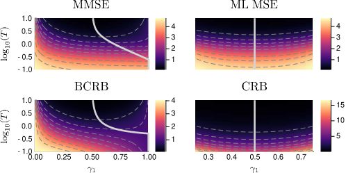
(a)

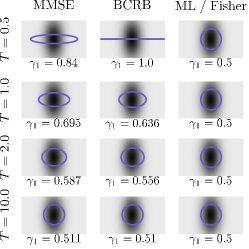
(b)

Figure 3: Encoding performance and optimal encoding in a two-dimensional uniform-Gaussian population with asymmetric prior $\sigma_{0,1}^{2}<\sigma_{0,2}^{2}$. Prior distribution as well as neuron-level and population-level energy constraints are the same in all subplots. (a) Performance criteria as a function of decoding time $T$ and tuning width ratio $\gamma_{1}=\alpha_{1}/\left(\alpha_{1}+\alpha_{2}\right)$. Contour levels are shown as dashed lines. Solid gray line indicates optimal width ratio $\gamma_{1}$. For the ML MSE and CRB, the $\gamma_{1}$ axis is clipped since these criteria approach infinity in each of the limits $\gamma_{1}\to 0$, $\gamma_{1}\to 1$. (b) Optimal encoding according to the various criteria (columns) over several decoding times (rows). A level set of the optimal tuning function is shown in blue, superimposed over the prior density. Optimal tuning width ratio is noted below each subplot. Parameters in all plots: $\bar{r}=2.5,2\pi\bar{h}=2,\Sigma_{0}=\mathrm{diag}\left(1,4\right)$.

The effect of the population-level energy constraint $\bar{r}$ is explored in Figure 4, where the optimality criteria are plotted as a function of $\bar{r}$ and the tuning width ratio $\gamma_{1}$, with the neuron-level constraint $\bar{h}$ and encoding time $T$ fixed. The prior variance $\Sigma_{0}$ in Figure 4 is narrower in dimension 1: $\sigma_{0,1}^{2}<\sigma_{0,2}^{2}$. As in Figure 3a, this produces an asymmetry in the opposite direction in the optimal tuning widths $\alpha_{1}^{2}>\alpha_{2}^{2}$, or equivalently, $\gamma_{1}>\frac{1}{2}$. Tuning is almost two-dimensional for low population rate constraint $\bar{r}$, becomes one-dimensional at intermediate population rates, and nearly two-dimensional again for high population rates. The BCRB correctly predicts $\gamma_{1}>\frac{1}{2}$ but fails to capture the dependence on the population constraint $\bar{r}$. The fact that the BCRB does not depend on $\bar{r}$ in the two-dimensional case may be seen by rewriting (24) for the case $m=2$ as

$$\mathrm{BCRB} =\left(\sigma_{0,1}^{-2}+h^{\prime}T\frac{\alpha_{2}}{\alpha_{1}}\right)^{-1}+\left(\sigma_{0,2}^{-2}+h^{\prime}T\frac{\alpha_{1}}{\alpha_{2}}\right)^{-1}$$

$$=\left(\sigma_{0,1}^{-2}+h^{\prime}T\left(\gamma_{1}^{-1}-1\right)\right)^{-1}+\left(\sigma_{0,2}^{-2}+\frac{h^{\prime}T}{\left(\gamma_{1}^{-1}-1\right)}\right)^{-1}$$

which for fixed $h^{\prime},T$ is strictly a function of $\gamma_{1}$.

Figure 5 shows the dependence of MSE-optimal tuning width ratio on prior asymmetry, quantified as the ratio $\sigma_{0,1}/\left(\sigma_{0,1}+\sigma_{0,2}\right)$, and on encoding time (left) or population-level energy constraint (right). Optimal tuning always has the opposite asymmetry to the prior. As seen on the left plot, optimal tuning is one-dimensional for short decoding time and becomes increasingly symmetric with increasing decoding time.

(a)

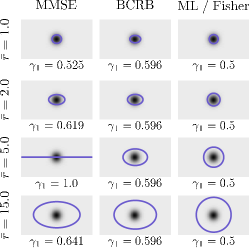
(b)

Figure 4: Encoding performance and optimal encoding as a function of population rate constraint $\bar{r}$ and tuning width ratio $\gamma_{1}$; see text and Figure 3 for details. Parameters are $T=1,2\pi\bar{h}=1.1$, $\Sigma_{0}=\mathrm{diag}\left(1,1.05\right)$.

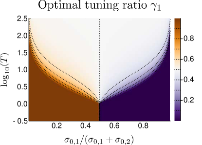
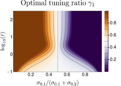
Figure 5: MMSE-optimal tuning width ratio $\gamma_{1}$ as a function of prior ratio $\sigma_{0,1}/\left(\sigma_{0,1}+\sigma_{0,2}\right)$ and encoding time (left) or population rate constraint (right), with the prior variance determinant $\det\Sigma_{0}=\sigma_{0,1}^{2}\sigma_{0,2}^{2}$ fixed. Parameters on the left are $\bar{r}=10,2\pi\bar{h}=1$, and on the right $T=1,2\pi\bar{h}=2$.

We compare our results to those obtained in [12] for a model of neural encoding of head-direction in bats. The encoding model in [12] includes neurons tuned to either one or both of two angles – azimuth or pitch. Preferred stimuli are drawn from a uniform distribution on the resulting torus. The estimation error of the ML estimator is compared in conjunctive (two-dimensional) coding, where each neuron encodes both directions, and pure (one-dimensional) coding, where each neuron encodes one of the dimensions. Their analysis predicts that in a large population, conjunctive coding always acheives lower error than pure coding, and this effect is stronger for shorter decoding time. Our finding that optimal coding is more symmetric for longer decoding time is the opposite of the conclusion in [12]. This discrepancy may be attributed to the use of ML estimation as opposed to MMSE, or to several differences between the models, as explored in more detail in appendix C.

6 Discussion

We have studied MMSE-optimal multivariate encoding for infinite uniform Gaussian neural population with population-level and neuron-level rate constraints. This formulation allows for closed-form evaluation of MMSE in the multivariate case (eqs. (9),(13)) as well as simple lower and upper bounds (16), and the derivation of analytic results regarding optimal tuning. Specifically, we have shown analytically that MMSE-optimal tuning functions in this model are aligned with the principal components of the prior distribution, and tuning is narrower in dimensions with larger prior variance. These analytic results allow for a more computationally efficient numerical optimization of encoding parameters, which we have used to evaluate the two-dimensional case in more detail. We have found that encoding only the dimension with higher variance is optimal for short encoding times (see Figure 3). We have also shown analytically that MSE-optimal multivariate encoding in our model always involves maximizing population firing rate, in contrast to the univariate case. This suggest that the population-level constraint is especially relevant in the multivariate setting. We have observed that optimal encoding depends in a non-trivial way on this rate constraint (see Figure 4).

Furthermore, the analytic tractability of the approach allows us to establish precise mathematical results, and to reach conceptually novel and intuitively interpretable conclusions that may be applicable to broader settings and to experimental data. Unfortunately, to the best of our knowledge, there are currently few experimental results on multivariate tuning properties that can be directly tested, but our results make concrete predictions (under admittedly restricted assumptions), when these become available.

Our framework differs from many previous studies in the direct optimization of decoding MMSE rather than proxies such as Fisher information or maximum likelihood estimation MSE, as well as in the explicit incorporation of population-level rate constraints. We have found that optimization of these proxies yields misleading results for short encoding times – as also observed in several previous works [4, 27, 19]. On the other hand, direct optimization of MMSE restricts the class of models where the objective function can be readily evaluated, since optimal decoding is generally intractable. To achieve mathematical tractability in the multivariate case, we have focused on the case of a Gaussian prior and Gaussian tuning functions that uniformly cover an unbounded stimulus space. Note that in this energy-constrained model, tuning width is also constrained, so that the effective space of preferred stimuli which are likely to fire under the Gaussian prior distribution of the state is bounded. Therefore, the unbounded space of preferred stimuli used in our framework does not rule out its applicability to biological settings with bounded stimulus space.

In the univariate case with a single neuron, closed-form MMSE has been previously derived in [6] for a wide class of tuning functions, under the assumption of uniform prior. Our work, in contrast, focuses on the case of uniform Gaussian tuning and Gaussian prior. Although this is a more restricted class of tuning functions, it facilitates analysis of the multivariate case. As far as we are aware, this work is the first that derives closed-form decoding MMSE for a multivariate stimulus. This suggests a possible direction for future research in the convergence of these approaches to study multivariate MMSE-optimal encoding for a wider class of tuning functions.

Appendix A Derivations

A.1 ML estimator

We have defined a modified ML estimator (17), which equals the prior mean when there are no spikes, since in this case the standard ML estimator is undefined under uniform coding. The MSE of this estimator may be computed directly from the law of total variance,

$$\mathbf{E}\left[\hat{X}_{t}^{\mathrm{ML}}|X,N_{t}=k\right] =\begin{cases}X&k\neq 0\\ \mu_{0}&k=0\end{cases}$$

$$\mathrm{Var}\left[\hat{X}_{t}^{\mathrm{ML}}|X,N_{t}=k\right] =\frac{1}{k^{2}}\mathrm{Var}\left[\sum_{i=1}^{k}\theta_{i}|X,N_{t}=k\right]=\frac{1}{k}R^{-1}\quad\left(k\neq 0\right)$$

$$\mathbf{E}\left[\left(X-\hat{X}_{t}^{\mathrm{ML}}\right)\left(X-\hat{X}_{t}^{\mathrm{ML}}\right)^{\mathsf{T}}\Big{|}X\right]$$

$$=\mathbf{E}\left[\mathrm{Var}\left[\hat{X}_{t}^{\mathrm{ML}}|X,N_{t}\right]|X\right]+\mathbf{E}\left[\left(\mathbf{E}\left[\hat{X}_{t}^{\mathrm{ML}}|X,N_{t}\right]-X\right)\left(\mathbf{E}\left[\hat{X}_{t}^{\mathrm{ML}}|X,N_{t}\right]-X\right)^{\mathsf{T}}\Big{|}X\right]$$

$$=\mathbf{E}\left[\frac{\mathbf{1}\left\{N_{t}>0\right\}}{N_{t}}\Big{|}X\right]R^{-1}+\mathbf{E}\left[\mathbf{1}\left\{N_{t}=0\right\}\left(\mu_{0}-X\right)\left(\mu_{0}-X\right)^{\mathsf{T}}\Big{|}X\right]$$

$$=e^{-rt}\left(\sum_{k=1}^{\infty}\frac{\left(rt\right)^{k}}{k!\,k}R^{-1}+\left(\mu_{0}-X\right)\left(\mu_{0}-X\right)^{\mathsf{T}}\right)$$ (34)

where $r$ is the population rate given by (6). In the diagonal case (11), we obtain the ML estimator’s conditional error by taking the trace of (34),

$$\epsilon\left(\hat{X}_{t}^{\mathrm{ML}}\big{|}X\right)=e^{-rt}\left[\sum_{k=1}^{\infty}\frac{\left(rt\right)^{k}}{k!\,k}\sum_{i=1}^{m}\alpha_{i}^{2}+\left|\mu_{0}-X\right|^{2}\right],$$

which yields the MSE (18) after taking the expected value.

A.2 Proofs

See 1

Proof.

Taking derivatives of (14) term by term yields the partial derivatives of $q\left(s,r\right)$,

$$q_{s}\left(s,r\right) =re^{-r}\sum_{k=0}^{\infty}\frac{r^{k}}{k!}\frac{1}{\left(s+k+1\right)^{2}},$$

$$q_{r}\left(s,r\right) =-se^{-r}\sum_{k=0}^{\infty}\frac{r^{k}}{k!}\frac{1}{\left(s+k\right)\left(s+k+1\right)},$$

from which a tedious but straightforward calculation yields

$$\frac{d}{d\alpha}q\left(c_{1}\alpha^{2},c_{2}\alpha^{m}\right) =e^{-r}\sum_{k=0}^{\infty}\frac{r^{k}}{k!}\frac{c_{1}c_{2}\alpha^{m+1}}{\left(s+k+1\right)^{2}}\left(2-m-\frac{m}{s+k}\right),$$

where $s=c_{1}\alpha^{2},r=c_{2}\alpha^{m}$. This derivative is clearly negative for positive $\alpha,c_{1},c_{2}$ and $m\geq 2$. ∎

See 2

As noted in section 5.1, applying this result to the prior precision $Q=\Sigma_{0}^{-1}$, the optimal tuning shape matrix $R=U\Lambda U^{\mathsf{T}}$ is a diagonal matrix with its diagonal elements in decreasing order. That is, tuning is aligned to the principal components, with narrower tuning (larger diagonal elements of $R$) for components with larger prior variance (smaller diagonal elements of $Q$).

Proof.

We first prove the claim for the case of distinct eigenvalues: $\lambda_{1}<\lambda_{2}<\cdots\lambda_{n}$ and $q_{1}<q_{2}<\cdots q_{n}$. We apply Lagrange multipliers to find necessary conditions on $U$. Using the fact that $\left(Q+U\Lambda U^{\mathsf{T}}\right)^{-1}$ is symmetric and the relations

$$\frac{\partial}{\partial X_{ij}}\mathrm{tr}\left[\left(Q+X\right)^{-1}\right] =-\left[\left(Q+X\right)^{-2}\right]_{ji}$$

$$\frac{\partial}{\partial U_{ij}}\left(UBU^{\mathsf{T}}\right)_{kl} =\left(J^{kl}UB^{\mathsf{T}}+J^{lk}UB\right)_{ij}$$

(e.g., [18, eqs. (64),(79)]), where $J^{kl}$ is the single-entry matrix $J_{ij}^{kl}\coloneqq\delta_{ik}\delta_{jl}$, we obtain

$$\frac{\partial}{\partial u_{ij}}\mathrm{tr}\left[\left(Q+U\Lambda U^{\mathsf{T}}\right)^{-1}\right]=-2\left[\left(Q+U\Lambda U^{\mathsf{T}}\right)^{-2}U\Lambda\right]_{ij}$$

The optimization constraints are $\sum_{s}u_{ks}u_{ls}=\delta_{kl}$ for $k,l\in\left\{1,\ldots n\right\}$. Differentiation of the $(k,l)$ constraint with respect to $u_{ij}$ yields

$$\frac{\partial}{\partial u_{ij}}\left[\sum_{s}u_{ks}u_{ls}-\delta_{kl}\right]=\delta_{ik}u_{lj}+\delta_{il}u_{kj}=\left[J^{kl}U+J^{lk}U\right]_{ij}$$

leading to the necessary condition

$$0=-2\left(Q+U\Lambda U^{\mathsf{T}}\right)^{-2}U\Lambda+\sum_{kl}\mu_{kl}\left(J^{kl}+J^{lk}\right)U,$$

where $\mu_{kl}$ are Lagrange multipliers. Multiplying on the right by $U^{\mathsf{T}}$ and using the constraint $UU^{\mathsf{T}}=I$ yields

$$\left(Q+U\Lambda U^{\mathsf{T}}\right)^{-2}U\Lambda U^{\mathsf{T}}=\frac{1}{2}\sum_{kl}\mu_{kl}\left(J^{kl}+J^{lk}\right).$$

The right-hand side is symmetric, therefore so is the left-hand side.

Let $R=U\Lambda U^{\mathsf{T}}$. We have found that $\left(Q+R\right)^{-2}R$ is symmetric, therefore $R$ commutes with $\left(Q+R\right)^{-2}$, and they share an orthogonal basis of eigenvectors. Since $R$’s eigenvalues are distinct, this basis is unique up to sign changes, so $(Q+R)^{-2}$ is also diagonalized by $U$, meaning $\left(Q+R\right)^{-2}=U\tilde{\Lambda}U^{\mathsf{T}}$ for some diagonal $\tilde{\Lambda}$. Now,

$$RQ =U\Lambda\left(\tilde{\Lambda}^{-1/2}-\Lambda\right)U^{\mathsf{T}}=U\left(\tilde{\Lambda}^{-1/2}-\Lambda\right)\Lambda U^{\mathsf{T}}=QR$$

so

$$q_{i}r_{ij}=\left(QR\right)_{ij}=\left(RQ\right)_{ij}=r_{ij}q_{j}.$$

and since $\left\{q_{i}\right\}$ are distinct and non-zero, $R$ is diagonal, $R=\mathrm{diag}\left(r_{1},\ldots r_{n}\right)$.

Since $R$ is diagonal and shares $\Lambda$’s eigenvalues, its diagonal is a permutation of $\Lambda$’s diagonal, i.e., $r_{i}=\lambda_{\pi\left(i\right)}$ for some permutation $\pi$ on $\left\{1,\ldots n\right\}$. Thus

$$r_{ij}=\delta_{ij}\lambda_{\pi\left(i\right)}=\sum_{k}\delta_{k,\pi\left(j\right)}\delta_{k,\pi\left(i\right)}\lambda_{k}=\left(P_{\pi}\Lambda P_{\pi}^{\mathsf{T}}\right)_{ij}$$

where $P_{\pi}$ is the permutation matrix $\left(P_{\pi}\right)_{ij}=\delta_{\pi\left(i\right),j}$. Since $U$ affects the objective function only through $R=U\Lambda U^{\mathsf{T}}$, any $U$ satisfying $U\Lambda U^{\mathsf{T}}=P_{\pi}\Lambda P_{\pi}^{\mathsf{T}}$ is optimal, and in particular, so is $U=P_{\pi}$ (and other optima are obtained by changing signs in $U$, $u_{ij}=\pm\left(P_{\pi}\right)_{ij}$).

The objective at the optimum is therefore of the form

$$\mathrm{tr}\left[\left(Q+R\right)^{-1}\right]=\sum_{i}\left(q_{i}+r_{i}\right)^{-1}=\sum_{i}\left(q_{i}+\lambda_{\pi\left(i\right)}\right)^{-1}.$$

To show that this is minimized by the inversion permutation $\pi\left(i\right)=n+1-i$, assume to the contrary that there are $i<j$ such that $\pi\left(i\right)<\pi\left(j\right)$. Denote by $\pi^{\prime}$ the permutation obtained from $\pi$ by switching these two elements,

$$\pi^{\prime}\left(k\right)=\begin{cases}\pi\left(j\right)&k=i\\ \pi\left(i\right)&k=j\\ \pi\left(k\right)&k\neq i,j\end{cases}$$

Since $i<j,\pi\left(i\right)<\pi\left(j\right)$ we have $q_{i}<q_{j}$ and $\lambda_{\pi\left(i\right)}<\lambda_{\pi\left(j\right)}$, therefore

$$\sum_{k}\left(q_{k}+\lambda_{\pi\left(k\right)}\right)^{-1}-\sum_{k}\left(q_{k}+\lambda_{\pi^{\prime}\left(k\right)}\right)^{-1}\\ =\left(\frac{1}{q_{i}+\lambda_{\pi\left(i\right)}}+\frac{1}{q_{j}+\lambda_{\pi\left(j\right)}}\right)-\left(\frac{1}{q_{i}+\lambda_{\pi\left(j\right)}}+\frac{1}{q_{j}+\lambda_{\pi\left(i\right)}}\right)\\ =\frac{q_{i}+q_{j}+\lambda_{\pi\left(i\right)}+\lambda_{\pi\left(j\right)}}{\left(q_{i}+\lambda_{\pi\left(i\right)}\right)\left(q_{j}+\lambda_{\pi\left(j\right)}\right)\left(q_{i}+\lambda_{\pi\left(j\right)}\right)\left(q_{j}+\lambda_{\pi\left(i\right)}\right)}\left(q_{j}-q_{i}\right)\left(\lambda_{\pi\left(j\right)}-\lambda_{\pi\left(i\right)}\right)>0,$$

contradicting the assumption that $P_{\pi}$ is optimal.

This concludes the proof for the case where all eigenvalues are distinct. The result is easily extended to the case of multiple eigenvalues by the continuity of the objective function: Denote the objective function for eigenvalues $\boldsymbol{q}=(q_{i})_{i=1}^{n},\boldsymbol{\lambda}=(\lambda_{i})_{i=1}^{n}$ by

$$f_{\boldsymbol{q},\boldsymbol{\lambda}}\left(U\right)\coloneqq\mathrm{tr}\left[\left(\mathrm{diag}\left(\boldsymbol{q}\right)+U\mathrm{diag}\left(\boldsymbol{\lambda}\right)U^{\mathsf{T}}\right)^{-1}\right].$$

Let $U^{*}$ denote the anti-diagonal $U$, which is optimal when eignevalues are distinct, and assume $U^{*}$ is not optimal for some $\boldsymbol{q}_{0},\boldsymbol{\lambda}_{0}$ (with possibly non-distinct elements), i.e., there is an orthogonal matrix $U^{\prime}$ such that $f_{\boldsymbol{q}_{0},\boldsymbol{\lambda}_{0}}\left(U^{\prime}\right)<f_{\boldsymbol{q}_{0},\boldsymbol{\lambda}_{0}}\left(U^{*}\right)$. Since $f$ depends continuously on $\boldsymbol{q},\boldsymbol{\lambda}$, this inequality holds in a neighborhood of $\boldsymbol{q}_{0},\boldsymbol{\lambda}_{0}$, which includes $\boldsymbol{q},\boldsymbol{\lambda}$ with distinct elements, contradicting the optimality result above. ∎

A.3 Fisher information of an infinite population

We derive Fisher information for an infinite neural population described by a marked point process with rate-density $\lambda\left(x;\theta\right)$, without assumptions on the form of $\lambda$, so the population might have non-Gaussian tuning and might be non-uniform.

Given an infinite population with rate-density $\lambda\left(x;\theta\right)$, the likelihood of a spike sequence $\left(t_{k},\theta_{k}\right)_{k=1}^{N_{T}}$ is given by

$$p\left(\left(t_{k},\theta_{k}\right)_{k=1}^{N_{T}}|X=x\right)=e^{-r\left(x\right)T}\prod_{k=1}^{N_{T}}\lambda\left(x;\theta_{k}\right),$$

where $r\left(x\right)\coloneqq\int\lambda\left(x;\theta\right)d\theta$ is the total population rate in response to $x$ (equation (5) is the special case of a uniform population, where the population rate $r\left(x\right)$ is constant). Denoting the log-likelihood by $L_{t}\left(x\right)$,

$$L_{t}\left(x\right) \coloneqq\log p\left(\left(t_{k},\theta_{k}\right)_{k=1}^{N_{T}}|X=x\right)=-r\left(x\right)T+\sum_{k=1}^{N_{T}}\log\lambda\left(x;\theta_{k}\right)$$

$$=-r\left(x\right)T+\int_{0}^{T}\int_{\mathbb{R}^{m}}\log\lambda\left(x;\theta\right)N\left(dt,d\theta\right).$$

Using the shorthand $\partial_{i}\coloneqq\partial/\partial x_{i}$, Fisher information is given by

$$J_{ij}\left(x\right) =-\mathbf{E}\left[\partial_{i}\partial_{j}L_{t}\left(x\right)|X=x\right]$$

$$=-\mathbf{E}\left[-\partial_{i}\partial_{j}r\left(x\right)+\int_{0}^{T}\int_{\mathbb{R}^{m}}\left(\partial_{i}\partial_{j}\log\lambda\left(x;\theta\right)\right)N\left(dt,d\theta\right)|X=x\right]$$

$$=T\partial_{i}\partial_{j}r\left(x\right)-T\int\left(\partial_{i}\partial_{j}\log\lambda\left(x;\theta\right)\right)\lambda\left(x;\theta\right)d\theta$$

$$=T\partial_{i}\partial_{j}r\left(x\right)-T\int\left(\partial_{i}\partial_{j}\lambda\left(x;\theta\right)-\frac{\left(\partial_{i}\lambda\left(x;\theta\right)\right)\left(\partial_{j}\lambda\left(x;\theta\right)\right)}{\lambda\left(x;\theta\right)}\right)d\theta$$

$$=T\int\frac{\left(\partial_{i}\lambda\left(x;\theta\right)\right)\left(\partial_{j}\lambda\left(x;\theta\right)\right)}{\lambda\left(x;\theta\right)}d\theta.$$

Appendix B Multiple sub-populations

To allow a more direct comparison to the analysis of [12], we extend our model in two ways. First, we consider $M$ uniform sub-population, each with its own maximal rate-density $h_{i}$ and tuning shape $R_{i}$. Second, the tuning in the $i$th sub-population takes the form

$$\lambda_{i}\left(x;\theta\right)\coloneqq h_{i}\exp\left(-\frac{1}{2}\left\|H_{i}x-\theta\right\|_{R_{i}}^{2}\right),$$ (35)

where the state dimensionality is now denoted $n$, and $H_{i}\in\mathbb{R}^{m_{i}\times n}$ is a matrix of full row rank ($m_{i}\leq n$), so that the sub-population encodes the linear projection $H_{i}x\in\mathbb{R}^{m_{i}}$ of the $n$-dimensional state to an $m_{i}$-dimensional subspace.

The derivation of the closed-form MMSE (9) can be readily extended to this case. The posterior Gaussian distribution has mean and variance

$$\mu_{T} =\Sigma_{T}\left(\Sigma_{0}^{-1}\mu_{0}+\sum_{j=1}^{M}H_{j}^{\mathsf{T}}R_{j}H_{j}\sum_{i=1}^{N_{T}^{\left(j\right)}}\theta_{i}^{\left(j\right)}\right),$$ (36)

$$\Sigma_{T} =\left(\Sigma_{0}^{-1}+\sum_{j=1}^{M}N_{T}^{\left(j\right)}H_{j}^{\mathsf{T}}R_{j}H_{j}\right)^{-1},$$ (37)

where $\theta_{i}^{\left(j\right)}$ is the preferred stimulus of the neuron firing the $i$-th spike from that population, and $N_{T}^{\left(j\right)}$ the number of spikes observed from the $j$-th population in the time interval $\left[0,T\right]$. Since $N_{T}^{\left(j\right)}$ are independent Poisson variables with rate

$$r_{j}=\sqrt{\frac{\left(2\pi\right)^{m_{j}}}{\det R_{j}}}h_{j},$$

the MMSE takes the form

$$\epsilon_{\mathrm{MMSE}} =\mathbf{E}\,\mathrm{tr}\left[\left(\Sigma_{0}^{-1}+\sum_{j=1}^{M}N_{T}^{\left(j\right)}H_{j}^{\mathsf{T}}R_{j}H_{j}\right)^{-1}\right]$$ (38)

$$=\exp\left(-\sum_{j=1}^{M}r_{j}T\right)\sum_{k_{1},\ldots k_{M}=0}^{\infty}\left[\prod_{j=1}^{M}\frac{\left(r_{j}T\right)^{k_{j}}}{k_{j}!}\right]\mathrm{tr}\left(\left(\Sigma_{0}^{-1}+\sum_{j=1}^{M}k_{j}H_{j}^{\mathsf{T}}R_{j}H_{j}\right){}^{-1}\right).$$ (39)

Fisher information in the $i$-th subpopulation is given by

$$J_{i}\left(x\right)=T\int\frac{\nabla_{x}\lambda_{i}\left(x;\theta\right)\nabla_{x}\lambda_{i}\left(x;\theta\right)^{\mathsf{T}}}{\lambda_{i}\left(x;\theta\right)}d\theta=h^{\prime}_{i}T\left|R_{i}\right|^{-1/2}H_{i}^{\mathsf{T}}R_{i}H_{i}=r_{i}TH_{i}^{\mathsf{T}}R_{i}H_{i}.$$ (40)

Since the subpopulations fire independently given the state $X$, Fisher information of the entire population is given by the sum $J\left(x\right)=\sum_{i}J_{i}\left(x\right)$.

For comparison with [12], we focus on the case of diagonal prior variance, with each sub-population encoding one of the dimensions. Specifically, assume the prior variance is diagonal (10), and the $j$-th subpopulation encodes only the $j$-th dimension, with tuning width $\alpha_{j}$, i.e., $H_{j}\in\mathbb{R}^{1\times n}$ is a row vector with

$$\left[H_{j}\right]_{1i}=\delta_{ij},\quad R_{j}=\alpha_{j}^{-2}.$$ (41)

The firing rate of the $j$-th subpopulation is

$$r_{j}=\sqrt{2\pi}\alpha h_{j},$$

and the MMSE is given by

$$\epsilon_{\mathrm{MMSE}} =\mathbf{E}\,\mathrm{tr}\left[\left(\Sigma_{0}^{-1}+\mathrm{diag}\left(\alpha_{1}^{-2}N_{T}^{\left(1\right)},\ldots,\alpha_{M}^{-2}N_{T}^{\left(M\right)}\right)\right){}^{-1}\right]$$

$$=\mathbf{E}\sum_{j=1}^{M}\frac{1}{\sigma_{0,j}^{-2}+\alpha_{j}^{-2}N_{T}^{\left(j\right)}}$$

$$=\sum_{j=1}^{M}\sigma_{0,j}^{2}q\left(\frac{\alpha_{j}^{2}}{\sigma_{0,j}^{2}},r_{j}\right)$$ (42)

where $q$ is defined in (14). Fisher information (40) under the setting (41) is given by

$$J\left(x\right) =\sum_{i=1}^{M}J_{i}\left(x\right)=\sum_{i=1}^{M}\frac{h^{\prime}_{i}T}{\alpha_{i}}H_{i}^{\mathsf{T}}H_{i}$$

$$=\mathrm{diag}\left(\frac{h_{1}^{\prime}T}{\alpha_{1}},\ldots\frac{h_{M}^{\prime}T}{\alpha_{M}}\right)=\mathrm{diag}\left(\frac{r_{1}T}{\alpha_{1}^{2}},\ldots\frac{r_{M}T}{\alpha_{M}^{2}}\right).$$

The ML estimator is generally not unique for the model (35) incorporating the projection matrix $H$. However, in the specific case (41), it is uniquely defined when there is at least one spike from each subpopulation. Analogously to the modified ML estimator for a single population defined in section 4.2, we define a modified ML estimator $\hat{X}_{t}^{\mathrm{ML}}=\left(\hat{X}_{t}^{1;\mathrm{ML}},\hat{X}_{t}^{2;\mathrm{ML}}\right),$ where the $i$-th dimension is estimated as

$$\hat{X}_{t}^{i;\mathrm{ML}}=\begin{cases}\frac{1}{N_{t}^{\left(i\right)}}\sum_{k=1}^{N_{t}^{\left(i\right)}}\theta_{k}^{\left(i\right)}&N_{t}^{\left(i\right)}>0,\\ \mu_{0,i}&N_{t}^{\left(i\right)}=0.\end{cases}$$ (43)

As in the single population case, this modified ML estimator may be obtained from the MMSE estimator (36) in the limit $\Sigma_{0}^{-1}\to 0$, and its MSE may be computed from the law of total variance,

$$\mathbf{E}\left[\hat{X}_{t}^{i;\mathrm{ML}}|X,N_{t}\right] =\begin{cases}X^{\left(i\right)},&N_{t}^{\left(i\right)}>0,\\ \mu_{0,i},&N_{t}^{\left(i\right)}=0,\end{cases}$$

$$\mathrm{Var}\left[\hat{X}_{t}^{i;\mathrm{ML}}|X,N_{t}\right] =\begin{cases}\alpha_{i}^{2}/N_{t}^{\left(i\right)},&N_{t}^{\left(i\right)}>0,\\ 0,&N_{t}^{\left(i\right)}=0.\end{cases}$$

$$\mathbf{E}\left[\left(X^{\left(i\right)}-\hat{X}_{t}^{i;\mathrm{ML}}\right)^{2}\Big{|}X\right]=\mathbf{E}\left[\mathrm{Var}\left[\hat{X}_{t}^{i;\mathrm{ML}}|X,N_{t}\right]|X\right]+\mathbf{E}\left[\left(\mathbf{E}\left[\hat{X}_{t}^{i;\mathrm{ML}}|X,N_{t}\right]-X^{\left(i\right)}\right)^{2}\Big{|}X\right]$$

$$=\mathbf{E}\left[\frac{\mathbf{1}\left\{N_{t}^{\left(i\right)}>0\right\}}{N_{t}^{\left(i\right)}}\Big{|}X\right]\alpha_{i}^{2}+\mathbf{E}\left[\mathbf{1}\left\{N_{t}^{\left(i\right)}=0\right\}\left(\mu_{0,i}-X^{\left(i\right)}\right)^{2}\Big{|}X\right]$$

$$=e^{-r_{i}t}\left(\sum_{k=1}^{\infty}\frac{\left(r_{i}t\right)^{k}}{k!\,k}\alpha_{i}^{2}+\left(\mu_{0,i}-X^{\left(i\right)}\right)^{2}\right).$$ (44)

Taking the expected value and summing over $i$ yields the MSE

$$\epsilon\left(\hat{X}_{t}^{\mathrm{ML}}\right)=\sum_{i=1}^{M}e^{-r_{i}t}\left[\left(\sum_{k=1}^{\infty}\frac{\left(r_{i}t\right)^{k}}{k!\,k}\right)\alpha_{i}^{2}+\sigma_{i}^{2}\right].$$ (45)

Appendix C Pure and conjunctive coding of two-dimensional stimuli

We compare our results to those obtained in [12] for a model of neural encoding of head-direction in bats. As noted in section 5.2, the encoding model in [12] includes neurons tuned to either one or both of two angles – azimuth or pitch. Preferred stimuli are drawn from a uniform distribution on the resulting torus. The estimation error of the ML estimator is compared in conjunctive (two-dimensional) coding, where each neuron encodes both directions, and pure (one-dimensional) coding, where each neuron encodes one of the dimensions. Their analysis predicts that in a large population, conjunctive coding always acheives lower error than pure coding, and this effect is stronger for shorter decoding time. This is in contrast to our finding that optimal coding is more symmetric for longer decoding time. This difference may be attributed to the use of ML estimation rather than MMSE estimation, or to several other differences between the models, as explained below.

To explore the difference between our results and those of [12], we focus on the case of symmetric prior and tuning, and compare the MMSE of conjunctive and pure encoding. Specifically, we compute the ratio of MMSE in conjunctive coding and MMSE in pure coding. We consider several variations of our model to bring it closer to that of [12]. Our model, as defined in the main text and studied in the two-dimensional case in section 5.2, differs from [12] in several ways:

Estimator

Optimal MMSE estimation vs. (suboptimal) ML esimation

State space

Encoding of a state in Euclidean space vs. encoding of angles

Number of subpopulations

A single population vs. two pure sub-populations

Subpopulation dimensionality

In our model, populations have preferred stimuli covering $\mathbb{R}^{2}$, but tuning curves may be arbitrarily thin and long. In [12], each pure populations has preferred stimuli covering a 1-d space and finite tuning width.

Normalization

Based on the derivation from firing rates constraints, we have considered populations with fixed firing rates $h,r$ and varying tuning widths. The model in [12] fixes the total rate $r$ and the tuning width $\alpha$ for pure and conjunctive encoding, resulting in different maximal firing rates per neuron between the two cases.

Since our framework allows computation of MMSE only for Euclidean state space, we do not address the problem of encoding of angles here. We therefore consider several possible definitions of the pure pouplation:

• A single pure population encoding one of the dimensions vs. two pure subpopulations each encoding one dimension

• The pure subpopulations are defined in one of three ways:

  1. 2-d pure populations ($\theta\in\mathbb{R}^{2}$) with same firing rates $h,r$ as in conjunctive code. MMSE is evaluated in the infinitely narrow limit $\alpha_{1}\to 0,\alpha_{2}\to\infty$ or vice versa. This is the setting studied in section 5.2.

  2. 1-d pure populations ($\theta\in\mathbb{R}$) with same firing rates $h,r$ as in conjunctive code. This setting allows finite population rates with finite tuning width $\alpha$, which is dictated by the rate constraints.

  3. 1-d pure populations ($\theta\in\mathbb{R}$) with same width $\alpha$ and population rate $r$ as in conjunctive code. In this case, the firing rate-density $h$ differs between pure and conjunctive coding.

More precisely, in the last two cases, each sub-population has tuning as given by (35) and (41). When there are two sub-populations, the firing rate $r$ that is equalized between pure and conjunctive coding is the total rate population rate, so that each sub-population has firing rate $r/2$. The errors for a single pure sub-population are calculated from the same equations ((13) and (42)) by assigning rate $r$ to one sub-population and rate 0 to the other.

MMSE ratio for pure vs. conjunctive coding in each of these six models as a function of encoding time is shown in Figure 6. Evidently, the preference for pure vs. conjunctive coding as a function of encoding time depends on the details of the model. The model of a single 2d pure population (top left) is the one appearing in the main text. The model of two 1d sub-populations with the same tuning width as the conjunctive population (bottom right) is the one most similar to [12]. In both these cases, we find that pure coding is relatively better for short decoding time, which is the opposite of the conclusion in [12].

	1 pure population	2 pure populations
2d
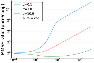
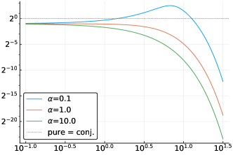
1d, same rate-density $h$
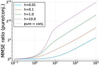
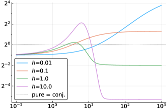
1d, same width $\alpha$

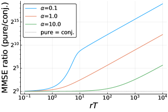
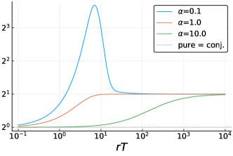
Figure 6: MMSE ratio of pure and conjunctive coding for various models. See text for more details. In the first row, each pure population is uniform in $\mathbb{R}^{2}$ with infinitely thin tuning. In the second row, each pure population is uniform in $\mathbb{R}$ and rate-density $h$ is the same for the pure and conjunctive codes. In the third row, each pure population is uniform in $\mathbb{R}$ and tuning width $\alpha$ is the same for the pure and conjunctive codes.

To assess whether the different dependence on encoding time is related to the use of ML estimation in [12], we also evaluate the ratio of ML MSE in pure and conjunctive coding for the models involving 1d pure populations in Figure 7. The model of a 2d pure population is omitted from this figure, since ML estimation in this model has infinite variance (as seen by taking the limit $\alpha_{1}\to 0,\alpha_{2}\to\infty$ in (18) with $r\propto\alpha_{1}\alpha_{2}$ fixed). The results for ML estimation are qualitatively similar to MMSE estimation in this symmetric case, except in some cases where pure coding achieves lower ML MSE than conjunctive coding, but worse MMSE (see, e.g., the bottom rows of Figures 6 and 7). In particular, pure coding remains preferable for short decoding time when using ML estimation.

	1 pure population	2 pure populations
1d, same rate-density $h$
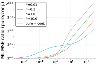
1d, same width $\alpha$

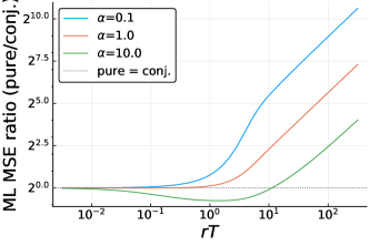
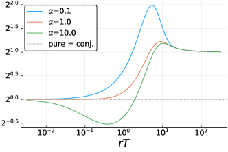
Figure 7: ML MSE ratio of pure and conjunctive coding for various models. See text and Figure 6 for more details.

This analysis suggests that the different conclusion in [12] is due to the cyclic nature of angle encoding. Experimentally observed tuning curves in [12] are quite wide relative to the range of possible angles, which might make a uniform population over the unbounded space $\mathbb{R}^{m}$ an inadequate model. In particular, the bounded space of angles allows for purely one-dimensional encoding with non-zero tuning width and finite population rate. A possible direction for future research is the analysis of MMSE-optimal encoding in a uniform population encoding angles.

References

- [1] George E Andrews, Richard Askey and Ranjan Roy “Special functions” 71, Encyclopedia of Mathematics and its Applications Cambridge university press, 2000
- [2] Andrea Benucci, Dario L Ringach and Matteo Carandini “Coding of stimulus sequences by population responses in visual cortex.” In Nature neuroscience 12.10, 2009, pp. 1317–1324 DOI: 10.1038/nn.2398
- [3] Pietro Berkes, Gergo Orbán, Máté Lengyel and József Fiser “Spontaneous cortical activity reveals hallmarks of an optimal internal model of the environment.” In Science (New York, N.Y.) 331.6013, 2011, pp. 83–7 DOI: 10.1126/science.1195870
- [4] Matthias Bethge, David Rotermund and Klaus Pawelzik “Optimal short-term population coding: when Fisher information fails.” In Neural Computation 14.10, 2002, pp. 2317–2351 DOI: 10.1162/08997660260293247
- [5] Matthias Bethge, David Rotermund and Klaus Pawelzik “Binary Tuning is Optimal for Neural Rate Coding with High Temporal Resolution”, 2003
- [6] Matthias Bethge, David Rotermund and Klaus Pawelzik “Optimal neural rate coding leads to bimodal firing rate distributions” In Network: Computation in Neural Systems 14.2, 2003, pp. 303–319 DOI: 10.1088/0954-898X_14_2_307
- [7] Matthias Bethge, David Rotermund and Klaus Pawelzik “Second Order Phase Transition in Neural Rate Coding: Binary Encoding is Optimal for Rapid Signal Transmission” In Physical Review Letters 90.8, 2003, pp. 088104 DOI: 10.1103/PhysRevLett.90.088104
- [8] Mohammad Darainy, Shahabeddin Vahdat and David J Ostry “Neural Basis of Sensorimotor Plasticity in Speech Motor Adaptation” In Cerebral Cortex, 2018, pp. 14
- [9] P. Dayan and L.F. Abbott “Theoretical Neuroscience: Computational and Mathematical Modeling of Neural Systems” MIT Press, 2005
- [10] I. Dean, B.. Robinson, N.. Harper and D. McAlpine “Rapid Neural Adaptation to Sound Level Statistics” In Journal of Neuroscience 28.25, 2008, pp. 6430–6438 DOI: 10.1523/JNEUROSCI.0470-08.2008
- [11] Christian W. Eurich and Stefan D. Wilke “Multidimensional encoding strategy of spiking neurons” In Neural Computation 12.7, 2000, pp. 1519–1529 DOI: 10.1162/089976600300015240
- [12] Arseny Finkelstein, Nachum Ulanovsky, Misha Tsodyks and Johnatan Aljadeff “Optimal dynamic coding by mixed-dimensionality neurons in the head-direction system of bats” In Nature Communications 9.1, 2018 DOI: 10.1038/s41467-018-05562-1
- [13] D. Ganguli and E.P. Simoncelli “Implicit encoding of prior probabilities in optimal neural populations” In Advances in neural information processing systems December 2010, 2011, pp. 6–9 arXiv:arXiv:1209.5006v1
- [14] Justin L. Gardner “Optimality and heuristics in perceptual neuroscience” In Nature Neuroscience, 2019 DOI: 10.1038/s41593-019-0340-4
- [15] Yuval Harel, Ron Meir and Manfred Opper “Optimal decoding of dynamic stimuli by heterogeneous populations of spiking neurons: A closed-form approximation” In Neural computation 30.8 MIT Press, 2018, pp. 2056–2112
- [16] N.S. Harper and D. McAlpine “Optimal neural population coding of an auditory spatial cue.” n1397b In Nature 430.7000, 2004, pp. 682–686 DOI: 10.1038/nature02768
- [17] Yudell L Luke “Inequalities for generalized hypergeometric functions” In Journal of Approximation Theory 5.1 Elsevier, 1972, pp. 41–65
- [18] Kaare Brandt Petersen and Syskind Pedersen Michael “The matrix cookbook”, 2004
- [19] Stevan Pilarski and Ondrej Pokora “On the Cramér-Rao bound applicability and the role of Fisher information in computational neuroscience” In BioSystems 136 Elsevier Ireland Ltd, 2015, pp. 11–22 DOI: 10.1016/j.biosystems.2015.07.009
- [20] DL Snyder, IB Rhodes and EV Hoversten “A separation theorem for stochastic control problems with point-process observations” In Automatica 13.1, 1977, pp. 85–87
- [21] Wensheng Sun and Dennis L. Barbour “Rate, not selectivity, determines neuronal population coding accuracy in auditory cortex” In PLoS Biology 15.11, 2017, pp. 1–22 DOI: 10.1371/journal.pbio.2002459
- [22] Alex Susemihl, Ron Meir and Manfred Opper “Analytical Results for the Error in Filtering of Gaussian Processes” In Advances in Neural Information Processing Systems 24, 2011, pp. 2303–2311
- [23] Alex Susemihl, Ron Meir and Manfred Opper “Dynamic state estimation based on Poisson spike trains—towards a theory of optimal encoding” In Journal of Statistical Mechanics: Theory and Experiment 2013.03 IOP Publishing, 2013, pp. P03009
- [24] Emanuel Todorov “Optimality principles in sensorimotor control” In Nature Neuroscience 7.9, 2004, pp. 907–915 DOI: 10.1038/nn1309
- [25] Harry L Van Trees “Detection, estimation, and modulation theory, part I: detection, estimation, and linear modulation theory” John Wiley & Sons, 2004
- [26] Zhuo Wang, Alan A Stocker and Daniel D Lee “Efficient neural codes that minimize lp reconstruction error” In Neural computation MIT Press, 2016
- [27] Steve Yaeli and Ron Meir “Error-based analysis of optimal tuning functions explains phenomena observed in sensory neurons.” In Front Comput Neurosci 4, 2010, pp. 130 DOI: 10.3389/fncom.2010.00130
- [28] Kechen Zhang and Terrence J Sejnowski “Neuronal Tuning: To Sharpen or Broaden?” In Biological Cybernetics 84, 1999, pp. 75–84