Multiple quadrotors carrying a flexible hose: dynamics, differential flatness, control

Abstract

Using quadrotors UAVs for cooperative payload transportation using cables has been actively gaining interest in the recent years. Understanding the dynamics of these complex multi-agent systems would help towards designing safe and reliable systems. In this work, we study one such multi-agent system comprising of multiple quadrotors transporting a flexible hose. We model the hose as a series of smaller discrete links and derive a generalized coordinate-free dynamics for the same. We show that certain configurations of this under-actuated system are differentially-flat. We linearize the dynamics using variation-based linearization and present a linear time-varying LQR to track desired trajectories. Finally, we present numerical simulations to validate the dynamics, flatness and control.

1 Introduction

Aerial manipulation has been an active research area for many years now, due to the simplicity of the dynamics and control of multi-rotors. The ubiquity of these aerial vehicles resulted in their use in a wide range of applications. Few such applications include search and rescue [Bernard et al. (2011)] and disaster management, for instance, using UAVs to monitor forest fires [Merino et al. (2012)]. Payload delivery using aerial vehicles [X-Wing (2019), PrimeAir (2019), Palunko et al. (2012)] is another application that has earned much attention in the last few years.

One extension of the payload carrying research is developing multi-rotor vehicles for active fire-fighting [Aerones (2018)] using a tethered hose that carries water and power. This enables carrying a fire hose to heights higher than a typical fire-truck ladder as well as fly longer due to the tethered power supply. Multi-rotors are also used to help string power cables between poles [SkyScopes (2017)], which typically is achieved using manned helicopters. To achieve stable and safe control of these complex systems, it is important to understand the underlying governing principles and dynamics. In this work, we aim to model and control the dynamics of a multiple quadrotor system carrying a flexible cable/hose.

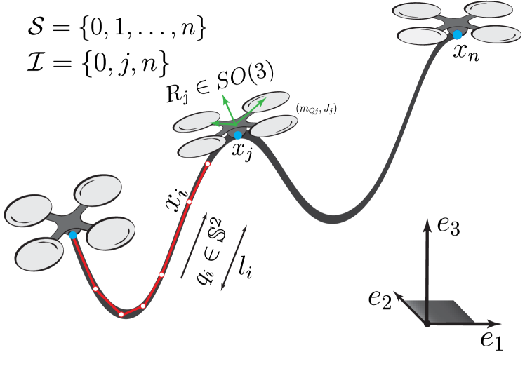
Figure 1: Multiple quadrotors carrying a flexible hose (with the hose modeled as a series of $n$ discrete-links). Links are massless with lumped mass at the ends and indexed through $\mathcal{S}=\{0,1,...,n\}$. The set $\mathcal{I}\subseteq\mathcal{S}$ gives the set of indices where the hose is attached to a quadrotor. Each link is modeled as a unit-vector $q_{i}\in\mathbb{S}^{2}$. The configuration space of this system is $Q:=\mathbb{R}^{3}\times(\mathbb{S}^{2})^{n}\times(SO(3))^{n_{Q}}$ $(n_{Q}=|\mathcal{I}|)$.

1.1 Related Work

There is a lot of literature on co-operative aerial manipulation, especially towards grasping and transporting payloads using multiple quadrotors [Maza et al. (2009), Mellinger et al. (2013), Jiang and Kumar (2012), Lee and Kim (2017), Michael et al. (2011)]. Trajectory tracking control for point-mass/rigid-body payloads suspended from multiple quadrotors is studied in [Lee et al. (2013), Goodarzi and Lee (2016), Sreenath and Kumar (2013), Wu and Sreenath (2014)]. Similarly, for loads suspended using flexible cables, stabilizing controllers are presented in [Goodarzi et al. (2015), Goodarzi and Lee (2015)] and these systems are shown to be differentially-flat in [Kotaru et al. (2018)]. Tethered aerial vehicles have also been extensively studied in the literature, for instance stabilization of tethered quadrotor and nonlinear-observers for the same are discussed in [Lupashin and D’Andrea (2013), Nicotra et al. (2014), Tognon and Franchi (2015)]. Geometric control of a tethered quadrotor with a flexible tether is presented in [Lee (2015)].

Most of the work discussed in the previous section models the tethers/cables either as rigid-links or as a series of links. Partial differential equations have also been used to model a continuous mass system, such as the aerial refueling cable shown in [Liu et al. (2017)]. However, modeling the aerial cable as a finite-segment lumped mass [Williams and Trivailo (2007), Ro and Kamman (2010)] is quite common in the literature due to the finite dimensionality of the state-space. However, most of these works assume Euler angles in the local frame to represent the attitude of the links. This results in complex equations of motion for the system that are also prone to singularities in case of aggressive motions. Therefore, in this work, we make use of coordinate-free representation that results in singularity-free and compact equations of motion.

1.2 Challenges

Multiple quadrotors carrying a flexible hose has multiple challenges in both modeling the dynamics and also designing a controller. Even though modeling the hose as a finite-segment lumped mass results in a finite-dimensional state space, it would still result in a large number of states depending on the choice of the number of discrete links. In addition, developing a controller is challenging due to the high under-actuation in the system. The swing of the cable, when not accounted for in the control, can have an adversarial effect.

1.3 Contributions

In this paper, we build upon the work done in the literature to develop the dynamics and control of multiple quadrotors carrying a flexible hose. This work is a step towards developing a system, with multiple quadrotor carrying a water-hose. However, for the purpose of this paper and as a first step, we consider no water flow in the hose. The contributions of this work are as follows,

• We derive a generalized coordinate-free dynamics for multiple quadrotors carrying a flexible hose  system. These dynamics can be extended to a tethered multiple quadrotor system.

• We show that this system is differentially-flat for certain configurations.

• We present variation-based linearized dynamics and implement a time-varying LQR to track a time-varying desired trajectory.

• Finally, we present numerical simulations to validate the dynamics and control.

To the best of authors knowledge, this is novel configuration of multiple quadrotors with a flexible hose and has not been studied prior to this work.

1.4 Organization

Rest of the paper is organized as follows. Section 2 explains the system definition, notations and presents the derivation of the dynamics. In Section 3 we show that the system is differentially-flat. In section 4, we present a LQR control on the variation-linearized dynamics. Section 5 presents numerical simulations validating the proposed controller. Finally, some of the limitations in this paper and potential directions to address them are discussed in Section 6. Concluding remarks are in Section 7.

2 Dynamics

Consider a flexible hose connected to multiple quadrotor UAVs as shown in Figure 1. In this section, we present the coordinate-free dynamics for this system. We consider the following assumptions before proceeding to derive the dynamics:

1. No water/water-flow in the hose and thus also no pressure forces;

2. Hose is modeled as a series of $n$ smaller links connected by spherical joints;

3. Each link is massless with lumped point-masses at the end with the hose mechanical properties like stiffness and torsional forces ignored.

4. The quadrotors attach to the hose at their respective center-of-masses.

In the following section, we present the notation used to describe the system.

2.1 Notation

Dynamics for the model are defined using geometric-representation of the states. Each link is a spherical-joint and is represented using a unit-vector $q\in\mathbb{S}^{2}:=\{x\in\mathbb{R}^{3}\leavevmode\nobreak\ |\leavevmode\nobreak\ \|x\|=1\}$. The position of one end of the cable is given in $\mathbb{R}^{3}$ and finally, the rotation matrix $R\in SO(3):=\{R\in\mathbb{R}^{3\times 3}|R^{\top}R=1,det(R)=+1\}$ is used to represent the attitude of the quadrotor.

Let the hose be discretized into $n$ links with the cable joints indexed as $\mathcal{S}=\{0,1,\ldots,n\}$ as shown in Figure 1. The position of one (starting) end of the hose is given as $x_{0}\in\mathbb{R}^{3}$ in the world-frame. The position of the link joints/point-masses is represented by $x_{i}\in\mathbb{R}^{3}$, where the link attitude between $x_{i{-}1}$ and $x_{i}$ is given by $q_{i}\in\mathbb{S}^{2}$ and length of this link-segment is $l_{i}$ i.e., $x_{i}=x_{i{-}1}{+}l_{i}q_{i}$. Also, $m_{i}$ is the mass of the lumped point-mass for link $i$. Let the set $\mathcal{I}\subseteq\mathcal{S}$ be the set of indices where the cable is attached to the quadrotor and $n_{Q}=|\mathcal{I}|$ is the number of quadrotors. For the $j^{th}$ quadrotor, $R_{j}\in SO(3)$ is the attitude, $m_{Qj},J_{j}$ is its mass and inertia matrix (in body-frame) and $f_{j}\in\mathbb{R},M_{j}\in\mathbb{R}^{3}$ are the corresponding thrust and moment for all $j\in\mathcal{I}$. Finally, the configuration space of this system is given as $Q:=\mathbb{R}^{3}\times(\mathbb{S}^{2})^{n}\times(SO(3))^{n_{Q}}$. Table 1 lists the various symbols used in this paper.

2.2 Derivation

The kinematic relation between the different link positions is given using link attitudes as,

$$x_{i}=x_{0}+\sum_{k=1}^{i}l_{k}q_{k}, \leavevmode\nobreak\ \forall\leavevmode\nobreak\ i\in\mathcal{S}\backslash\{0\},$$ (1)

and the corresponding velocities and accelerations are related as,

$$v_{i}=v_{0}+\textstyle\sum_{k=1}^{i}l_{k}\dot{q}_{k},\quad a_{i}=a_{0}+\textstyle\sum_{k=1}^{i}l_{k}\ddot{q}_{k}.$$ (2)

Potential energy $\mathcal{U}:TQ\rightarrow\mathbb{R}$ of the system, due to hose and quadrotors’ mass is computed as shown below,

$$\mathcal{U}=\sum_{i\in\mathcal{S}}\overline{m}_{i}x_{i}\cdot g\bm{e_{3}},$$ (3)

where $\overline{m}_{i}=m_{i}+m_{Qi}\mathbf{1}_{i}$ is the net-mass at index $i$ and $\mathbf{1}_{i}:=\mathbf{1}_{\mathcal{I}}(i)=\begin{cases}1,\leavevmode\nobreak\ \textit{if }i\in\mathcal{I}\\ 0,\leavevmode\nobreak\ \textit{else}\end{cases}$ is an indicator function for the set $\mathcal{I}$.

Kinetic energy $\mathcal{T}:TQ\rightarrow\mathbb{R}$ is similarly given as,

$$\mathcal{T}=\sum_{i\in\mathcal{S}}\frac{1}{2}\overline{m}_{i}\langle v_{i},v_{i}\rangle+\sum_{j\in\mathcal{I}}\frac{1}{2}\langle\Omega_{j},J_{j}\Omega_{j}\rangle,$$ (7)

where $\Omega_{j}$ is the angular velocity of the quadrotor $j$ in its body-frame. Dynamics of the system are derived using the Lagrangian method, where Lagrangian $\mathcal{L}:TQ\rightarrow\mathbb{R}$, is given as,

$$\mathcal{L}=\mathcal{T}-\mathcal{U}.$$

We derive the equations of motion using the Langrange-d’Alembert principle of least action, given below,

$$\delta\int_{t_{0}}^{t_{f}}\mathcal{L}dt+\int_{t_{0}}^{t_{f}}\delta W_{e}dt=0,$$ (8)

where $\delta W_{e}$ is the infinitesimal work done by the external forces. $\delta W_{e}$ can be computed as,

$$\delta W_{e} =\sum_{j\in\mathcal{I}}\Big{(}\langle W_{1,j},\hat{M}_{j}\rangle+\langle W_{2,j},f_{j}R_{j}\bm{e_{3}}\rangle\Big{)},$$ (9)

$$W_{1,j}=R^{T}_{j}\delta R_{j},$$ (10)

$$W_{2,j}=\delta x_{j}=\delta x_{0}+\textstyle\sum_{k=1}^{j}l_{k}\delta q_{k},$$ (11)

are variational vector fields [Goodarzi et al. (2015)] corresponding to quadrotor attitudes and positions. The infinitesimal variations on $q$ and $R$ are expressed as,

$$\delta q={\xi}^{\times}q=-{q}^{\times}\xi,\leavevmode\nobreak\ \xi\in\mathbb{R}^{3}\leavevmode\nobreak\ \text{s.t.}\leavevmode\nobreak\ \xi\cdot q=0,$$

$$\delta\dot{q}={-}{q}^{\times}\dot{\xi}{-}{\dot{q}}^{\times}\xi,$$

$$\delta R=R{\eta}^{\times},\quad\delta{\Omega}^{\times}={({\Omega}^{\times}\eta)}^{\times}{+}{\dot{\eta}}^{\times},\eta\in\mathbb{R}^{3},$$

with the constraints $q\cdot\dot{q}=0$ and $q\cdot{\omega}=0$, $\omega$ is the angular velocity of $q$, s.t. $\dot{q}=\omega\times q$. The cross-map is defined as ${(\cdot)}^{\times}:\mathbb{R}^{3}\rightarrow\mathbf{so(3)}$ s.t ${x}^{\times}y=x\times y,\forall x,y\in\mathbb{R}^{3}$. Similarly, variations on the link positions are given as,

$$\delta x_{i}=\delta x_{0}+\sum_{k=1}^{i}l_{k}\delta q_{k}=\delta x_{0}{-}\sum_{k=1}^{i}l_{k}{q}^{\times}_{k}\xi_{k},$$ (12)

$$\delta v_{i}=\delta v_{0}{+}\sum_{k=1}^{i}l_{k}\delta\dot{q}_{k}=\delta v_{0}{-}\sum_{k=1}^{i}l_{k}({q}^{\times}_{k}\dot{\xi_{k}}{+}{\dot{q}}^{\times}_{k}\xi_{k}).$$ (13)

Finally, we obtain the equations of motion for the system by solving (8). See Appendix A for the detailed derivation. Equations of motion for the multiple quadrotors carrying a flexible hose are given in (4)-(6). Note the mass-matrix $\mathbb{M}_{\{q_{i}\}}$ is a function of link attitudes $\{q_{i}\}=\{q_{1},q_{2},\ldots q_{n}\}$ and we use the following notation similar to [Goodarzi et al. (2014)]

$$M_{00}{=}\textstyle\sum_{k=0}^{n}\overline{m}_{k},M_{0i}{=}l_{i}\textstyle\sum_{k=i}^{n}\overline{m}_{k},$$

$$M_{i0}{=}M_{0i},M_{ij}=\textstyle\sum_{k=\max\{ij\}}^{n}\overline{m}_{k}l_{i}l_{j}.$$ (14)

Remark: 1

In (5), note the use of $f_{i},R_{i}$ for $i\notin\mathcal{I}$, (since $i\notin\mathcal{I}$ implies no quadrotor is attached at index $i$ and thus cannot have $f_{i}$ and $R_{i}$). However, this notation is used for convenience, since $i{\notin}\mathcal{I}{\implies}\mathbf{1}_{i}{=}0$ and thus $f_{i}R_{i}\bm{e_{3}}\mathbf{1}_{i}=0$, there by ensuring the right inputs to the system.

Remark: 2

Degrees of freedom for the multiple quadrotors carrying a flexible hose  is $DOF=3(n_{Q}{+}1){+}2n$ where $2n$ corresponds to the link attitudes DOF, $3n_{Q}$ the rotational DOF of the quadrotors and $3$ for the initial position $x_{0}$. Similarly, the degrees of actuation is $DOA=4n_{Q}$ corresponding to the $4$ inputs for each quadrotor. Thus, the degrees of under-actuation are $DOuA=2n+3-n_{Q}$. For a typical setup we have $n>>n_{Q}$, i.e., system is highly under-actuated.

Remark: 3

For a tethered system, we can assume $x_{0}{\equiv}0$ $\forall\leavevmode\nobreak\ t$, i.e. the system is tethered to origin of the inertial frame, and we can derive the dynamics as earlier. Equations of motion for this system would be same as (4)-(6), without the equation corresponding to $\dot{v}_{0}$.

Table 1: List of various symbols used in this work. Note: $k{\in}\mathcal{S},i{\in}\mathcal{S}\backslash\{0\},j{\in}\mathcal{I}$, WF - World frame, BF-Body-frame, $|\cdot|$ represents cardinality of a set.

Variables	Definition
$n\in\mathbb{R}^{+}$	Number of links in the hose.
$\mathcal{S}=\{0,1,\ldots,n\}$	Set containing indices of the hose-segments.
$x_{k}\in\mathbb{R}^{3}$	Position of the $k^{th}$ point-mass of the hose in WF.
$v_{k}\in\mathbb{R}^{3}$	Velocity of the $k^{th}$ point-mass of the hose in WF.
$l_{i}\in\mathbb{R}^{+}$	Length of the $i^{th}$ segment.
$m_{k}\in\mathbb{R}^{+}$	Mass of the $k^{th}$ point-mass in the hose-segments.
$q_{i}\in\mathbb{S}^{2}$	Orientation of the $i^{th}$ hose segment in WF.
$\omega_{i}\in T_{q_{i}}\mathbb{S}^{2}$	Angular velocity of the $i^{th}$ hose segment in WF.
$\mathcal{I}\subset\mathcal{S}$	Set of indices where the hose is attached to the quadrotor.
$|\mathcal{I}|=n_{Q}$	Number of quadrotors.
$x_{Qj}\equiv x_{j}$	Center-of-mass position of the $j^{th}$ quadrotor in WF.
$R_{j}\in SO(3)$	Attitude of the $j^{th}$ quadrotor w.r.t. WF.
$\Omega_{j}\in T_{R_{j}}SO(3)$	Angular velocity of the $j^{th}$ quadrotor in BF.
$m_{Qj}$, $J_{j}$	Mass & inertia of the $j^{th}$ quadrotor.
$f_{j}\in\mathbb{R},\leavevmode\nobreak\ M_{j}\in\mathbb{R}^{3}$	Thrust and moment of the $j^{th}$ quadrotor in BF.
$\mathbf{1}_{i}:=\mathbf{1}_{\mathcal{I}}(i)=\begin{cases}1\leavevmode\nobreak\ \textit{if }i\in\mathcal{I}\\ 0\leavevmode\nobreak\ \textit{else}\end{cases}$	Indicator function for the set $\mathcal{I}$.
$\overline{m}_{k}=m_{k}+m_{Qk}\mathbf{1}_{k}$	Net mass at the $k^{th}$ link joint.
$u_{k}=(-{\overline{m}_{k}}g\bm{e_{3}}+f_{k}R_{k}\bm{e_{3}}\mathbf{1}_{k})$	Net force due to thrusters & gravity.

3 Differential Flatness

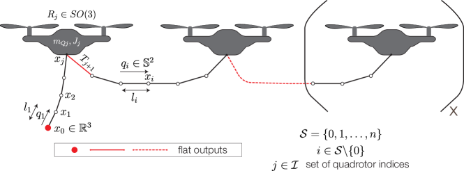
Figure 2: Configuration of the multiple quadrotors carrying a flexible hose illustrating the differential-flatness and its flat-outputs (shown in red).

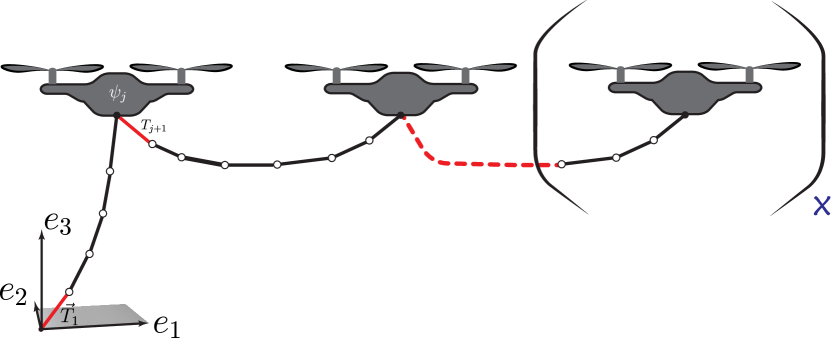
Figure 3: Tethered multiple quadrotors carrying a flexible hose.

In the previous section, we derived the dynamics for multiple quadrotors carrying a flexible hose. The system is under-actuated and thus the control of the system is challenging. In this section, we show that the system is differentially-flat. A nonlinear system is differentially-flat if a set of outputs of the system (equal to the number of inputs) and their derivatives can be used to determine the states and inputs without integration.

Definition: 1

Differentially-Flat System, [Murray et al. (1995)]: A system $\dot{\mathbf{x}}=f(\mathbf{x},\mathbf{u}),\,\mathbf{x}\in\mathbb{R}^{n},\,\mathbf{u}\in\mathbb{R}^{m},\,$ is differentially flat if there exists flat outputs $\mathbf{y}\in\mathbb{R}^{m}$ of the form $\mathbf{y}=\mathbf{y}(\mathbf{x},\mathbf{u},\dot{\mathbf{u}},\ldots,\mathbf{u}^{(\mathbf{p})})$ such that the states and the inputs can be expressed as $\mathbf{x}=\mathbf{x}(\mathbf{y},\dot{\mathbf{y}},\ldots,\mathbf{y}^{\mathbf{(q)}})$, $\mathbf{u}=\mathbf{u}(\mathbf{y},\dot{\mathbf{y}},\ldots,\mathbf{y}^{(\mathbf{q})})$, where $\mathbf{p},\,\mathbf{q}$ are positive finite integers.

A quadrotor is a differentially-flat system with the quadrotor center-of-mass and yaw as the flat outputs [Mellinger and Kumar (2011)]. A quadrotor with cable suspended load (with the cable modeled as a massless link) is also shown to be differentially-flat with load position and quadrotor yaw as the flat outputs [Sreenath et al. (2013)]. Similarly, a quadrotor with flexible cable suspended load, with the cable modeled as series of smaller links is shown to be differentially-flat [Kotaru et al. (2018)]. Again, here load position and quadrotor yaw are the flat-outputs. For the system defined in this work, the quadorotor-flexible cable segments are connected in series. Unlike previous work where each quadrotor has only one segment connected to it, each quadrotor in this system can have $0,1,$ or $2$ segments connected to it. In the following, we formalize the differential-flatness for certain configurations of the multiple quadrotors carrying a flexible hose system.

Lemma

${\pazocal{Y}=(x_{0},\psi_{j},T_{k{+}1})}\leavevmode\nobreak\ \forall j{\in}\mathcal{I}\leavevmode\nobreak\ \&\leavevmode\nobreak\ k{\in}\mathcal{I}\backslash\{n\}$ are the set of flat-outputs for multiple quadrotors carrying a flexible hose with $n{\in}\mathcal{I}$ (i.e., end of the cable is always attached to a quadrotor as shown in Figure 2), where $x_{0}{\in}\mathbb{R}^{3}$ is the position of the start of the cable, $\psi_{j}{\in}\mathbb{R}$ is the yaw angle of the $j^{th}$ quadrotor and $T_{k+1}\in\mathbb{R}^{3}$ is the tension vector in the $(k{+}1)^{th}$ link (as shown in Figure 2).

See Appendix B

Remark: 4

To determine the states and inputs of the system with $n-$ links, requires $(2n{+}4)$ derivatives of the flat-output $x_{0}$, $2^{nd}$ derivative of the yaw angle $\psi_{j}$ and $2(n{-}k){+}2$ derivatives of the tension vector $T_{k{+}1}$.

Corollary 1

$\pazocal{Y}=(T_{1},\psi_{j},T_{k{+}1})\leavevmode\nobreak\ \forall j{\in}\mathcal{I}\leavevmode\nobreak\ \&\leavevmode\nobreak\ k{\in}\mathcal{I}\backslash\{n\}$ are the flat-outputs for a tethered multiple quadrotors carrying a flexible hose shown in Figure 3, where $T_{1}\in\mathbb{R}^{3}$ is the tension in the $1^{st}$ link, $\psi_{j}\in\mathbb{R}$ is the yaw angle of the quadrotor at index $j$ and $T_{k+1}\in\mathbb{R}^{3}$ is the tension vector in the $(k{+}1)^{th}$ link.

See Appendix B

Differential-flatness is used in planning the system trajectories, where the flat outputs are used to plan in the lower-dimension space and the corresponding desired states and inputs are computed using differential flatness. In the next section, we present the linearized dynamics about any desired time-varying trajectory and use an LQR to track desired trajectories.

4 Control

Having presented differential-flatness in the previous section, we proceed to present control to track desired-trajectories generated using the flat-outputs in this section. As presented in the Remark 2, the given system is highly underactuated and thus controlling the system is challenging. In this section, we present a way to control the system by linearizing the dynamics in (4)-(6) about a given desired time-varying trajectory $(x_{0d}(t),v_{0d}(t),q_{id}(t),\omega_{id}(t),R_{jd}(t),\Omega_{jd}(t))$, $\forall i\in\mathcal{S},j\in\mathcal{I}$ and then implementing a linear controller.

4.1 Variation Based Linearization

In this sub-section, we present the coordinate-free linear dynamics, obtained through variation based linearization of the nonlinear dynamics in (4)-(6). We use the variation linearization techniques described in [Wu and Sreenath (2015)] to obtain the linear dynamics. The error state of the linear-dynamics is given as,

$$\mathbf{\delta x} =[\delta x,\leavevmode\nobreak\ \xi_{1},\leavevmode\nobreak\ \ldots,\leavevmode\nobreak\ \xi_{n},\leavevmode\nobreak\ \delta v,\leavevmode\nobreak\ \delta\omega_{1},\leavevmode\nobreak\ \ldots,\delta\omega_{n},$$

$$\quad\quad\eta_{j_{1}},\leavevmode\nobreak\ \ldots,\leavevmode\nobreak\ \eta_{j_{n_{Q}}},\leavevmode\nobreak\ \delta\Omega_{j_{1}},\leavevmode\nobreak\ \ldots,\leavevmode\nobreak\ \delta\Omega_{j_{n_{Q}}}]^{\top},$$ (15)

and the corresponding inputs as,

$$\mathbf{\delta u} =[\delta f_{j_{1}},\delta f_{j_{2}},\ldots,\delta f_{j_{n_{Q}}},\delta M_{j_{1}}^{\top},\delta M_{j_{2}}^{\top},..,\delta M_{j_{n_{Q}}}^{\top}]^{\top},$$ (16)

where $j_{1},j_{2},\ldots,j_{n_{Q}}$ are elements of $\mathcal{I}$ arranged in increasing order. The individual elements of the error state are computed as,

$$\delta x=x{-}x_{d},\leavevmode\nobreak\ \delta v=v{-}v_{d},$$

$$\xi_{i}={q}^{\times}_{id}q_{i},\leavevmode\nobreak\ \delta\omega_{i}=\omega_{i}-(-({q}^{\times}_{i})^{2})\omega_{id},$$

$$\eta_{j}=\frac{1}{2}{(R_{jd}^{T}R_{j}-R_{j}^{T}R_{jd})}^{\vee},\leavevmode\nobreak\ \delta\Omega_{j}=\Omega_{j}-R_{j}^{T}R_{jd}\Omega_{jd}.$$

Finally, the linearized dynamics (See Appendix C for detailed derivation of the linearized dynamics) about a time-varying desired trajectory are given below,

$$\delta\dot{\mathbf{x}}=\mathcal{A}\delta\mathbf{x}+\mathcal{B}\delta\mathbf{u},$$ (17)

$$\mathcal{C}\delta\mathbf{x}=0.$$ (18)

The linear dynamics matrices $\mathcal{A,B}$ are,

$$\mathcal{A}{=}\begin{bmatrix}0_{3,3}&0_{3,3n}&I_{3,3}&0_{3,3n}&0_{3,3n_{Q}}&0_{3,3n_{Q}}\\ 0_{3n,3}&\alpha&0_{3,3}&\beta&0_{3,3n_{Q}}&0_{3,3n_{Q}}\\ &&&\mathbb{M}_{\{q_{id}\}}^{-1}F&\\ 0_{3n_{Q},3}&0_{3n_{Q},3n}&0_{3n_{Q},3}&0_{3n_{Q},3n}&\gamma&I_{3n_{Q},3n_{Q}}\\ 0_{3n_{Q},3}&0_{3n_{Q},3n}&0_{3n_{Q},3}&0_{3n_{Q},3n}&0_{3n_{Q},3n_{Q}}&\nu\end{bmatrix},$$ (19)

with,

$$F=\begin{bmatrix}O_{3,3}&[a]_{i}&O_{3,3}&[b]_{i}&[e]_{j}&O_{3n_{Q},3n_{Q}}\\ O_{3n,3}&[c]_{i,j}&O_{3n,3}&[d]_{i,j}&[f]_{i,j}&O_{3n_{Q},3n_{Q}}\end{bmatrix},$$

$$\alpha=\textit{bdiag}[q_{1d}q_{1d}^{\top}{\omega}^{\times}_{1d},\leavevmode\nobreak\ q_{2d}q_{2d}^{\top}{\omega}^{\times}_{2d},\leavevmode\nobreak\ \ldots,\leavevmode\nobreak\ q_{nd}q_{nd}^{\top}{\omega}^{\times}_{nd}],$$

$$\beta=\textit{bdiag}[\big{(}I_{3}{-}q_{1d}q_{1d}^{\top}\big{)},\big{(}I_{3}{-}q_{2d}q_{2d}^{\top}\big{)},\ldots,\big{(}I_{3}{-}q_{nd}q_{nd}^{\top}\big{)}],$$

$$\gamma=\textit{bdiag}[-{\Omega}^{\times}_{j1d},\leavevmode\nobreak\ -{\Omega}^{\times}_{j2d},\ldots,-{\Omega}^{\times}_{jn_{Q}d}],$$

$$\nu=\textit{bdiag}[J_{1}^{-1}({(J_{1}\Omega_{1d})}^{\times}{-}{\Omega}^{\times}_{1d}J_{1}),\ldots,J_{n}^{-1}({(J_{n}\Omega_{nd})}^{\times}{-}{\Omega}^{\times}_{nd}J_{n})],$$

and

$$\mathcal{B}=\begin{bmatrix}O_{3(n{+}1),4n_{Q}}\\ \mathbb{M}_{\{q_{id}\}}^{-1}G\\ O_{3n_{Q},4n_{Q}}\\ \begin{bmatrix}O_{3n_{Q},n_{Q}}&\mu\end{bmatrix}\end{bmatrix},\text{ with }\mu=\textit{bdiag}[J^{-1}_{j1},\ldots,J^{-1}_{jn_{Q}}],$$ (20)

$$G=\begin{bmatrix}\left.\begin{matrix}[g]_{i}\\ [h]_{i,j}\end{matrix}\right|&O_{(3(n+1),3n_{Q})}\end{bmatrix}.$$

Next, the constraint matrix $\mathcal{C}$ is defined as,

$$\mathcal{C}{=}\begin{bmatrix}O_{n,3}&\mathcal{C}_{1}&O_{n,3}&O_{n,3n}&O_{n,6n_{Q}}\\ O_{n,3}&\mathcal{C}_{2}&O_{n,3}&\mathcal{C}_{1}&O_{n,6n_{Q}}\end{bmatrix},$$ (21)

with

$$\mathcal{C}_{1}=bdiag(q^{T}_{1d},q^{T}_{2d},\ldots,q^{T}_{nd}),\mathcal{C}_{2}=bdiag({-}\omega^{T}_{1d}{q}^{\times}_{1d},\ldots,{-}\omega^{T}_{nd}{q}^{\times}_{nd}).$$

The rest of the elements are described below,

$$a_{i} =M_{0i}\big{[}({\dot{\omega}}^{\times}_{id}-\|\omega_{id}\|^{2}I_{3}){q}^{\times}_{id},$$

$$b_{i} =M_{0i}(2q_{id}\omega_{id}^{\top}),\quad i=\{1,\ldots,n\},$$

$$c_{ij} =\begin{cases}\big{[}M_{io}{\dot{v}_{0d}}^{\times}-\sum_{j=1,j\neq i}^{n}M_{ij}\big{(}{({q}^{\times}_{jd})\dot{\omega}_{jd})}^{\times}+\\ \quad\quad\quad\|\omega_{jd}\|^{2}{q}^{\times}_{jd}\big{)}-l_{i}{\big{(}\sum_{k=i}^{n}{u}^{\times}_{k}\big{)}}\big{]}(-{q}^{\times}_{i}),&\quad i=j\\ \big{[}M_{ij}{q}^{\times}_{id}\big{(}{\dot{\omega}}^{\times}_{jd}-\|\omega_{jd}\|^{2}I\big{)}{q}^{\times}_{jd}\big{]},&\quad i\neq j\end{cases}$$

$$d_{ij} =\begin{cases}O_{3,3},&\quad i=j\\ M_{ij}\big{[}2{q}^{\times}_{id}q_{jd}\omega^{\top}_{jd}\big{]},&\quad i\neq j\end{cases}$$

$$e_{j} =-f_{jd}R_{jd}{e}^{\times}_{3},\quad j\in{\mathcal{I}}$$

$$f_{ij} =\begin{cases}\phi,&if\leavevmode\nobreak\ j\notin\mathcal{I}\\ -(l_{i}{q}^{\times}_{i})f_{jd}R_{jd}{e_{3}}^{\times},&if\leavevmode\nobreak\ j\in\mathcal{I},j\geq i\\ O_{3,3},&if\leavevmode\nobreak\ j\in\mathcal{I},j<i\end{cases}$$

$$g_{j} =R_{jd}e_{3},$$

$$h_{ij} =\begin{cases}\phi,&if\leavevmode\nobreak\ j\notin\mathcal{I}\\ (l_{i}{q}^{\times}_{i})R_{jd}{e_{3}},&if\leavevmode\nobreak\ j\in\mathcal{I},j\geq i\\ O_{3,1},&if\leavevmode\nobreak\ j\in\mathcal{I},j<i\end{cases}$$

and bdiag is block diagonal matrix. Note that $\mathbb{M}_{\{q_{id}\}}$ in (19), (20) is the same mass matrix in (5), except is the function of desired link attitudes $\{q_{id}\}$.

As seen, (17)-(18) is a time-varying constrained linear system. The constraints arise due to the variation constraint on $S^{2}$ as discussed in [Wu and Sreenath (2015)]. Controllability of the constrained linear equation can be shown similar to [Wu and Sreenath (2015)], however, due the complexity of the matrices $\mathcal{A,B,C}$ computing the controllability matrix would be intractable.

4.2 Finite-Horizon LQR

Assuming, we have the complete reference trajectory we can implement any linear control technique for (17)-(18). Similar to [(Wu and Sreenath, 2015, Lemma 1)], we can show that the constraint (18) is time-invariant, i.e., if the initial condition satisfies the constraint, solution to the linear system would satisfy the constraint for all time. However, due to this constraint, the controllability matrix computed using $\mathcal{A,B}$ might not be full-rank and requires state transformation into the unconstrained space to result in full-rank controllability matrix.

Instead, we opt for a finite-horizon LQR controller for the variation-linearized dynamics about a time-varying desired trajectory. We chose a finite-time horizon $T$, the terminal cost matrix $P_{T}$ and pick cost matrices for states $Q_{1}=Q_{1}^{T}$ and inputs $Q_{2}=Q_{2}^{T}$. Finally, we solve the continuous-time Ricatti equation backwards in time to obtain the gain matrix $P(t)$, that satisfies,

$$-\dot{P}=Q_{1}-P\mathcal{B}Q_{2}^{-1}\mathcal{B}^{T}P+\mathcal{A}^{T}P+P\mathcal{A}.$$ (22)

The above equation is solved offline and stored in a table for online computation. Note that the explicit time dependence of $P,\mathcal{A},\mathcal{B}$ is dropped for convenience. Finally, the feedback gain for the control input is computed as,

$$K=R^{-1}\mathcal{B}P,\quad\delta\mathbf{u}=-K\delta\mathbf{x}.$$ (23)

Since the gains are computed backwards in time, the computed input would result in a stable control for the constrained linear-system. The net control-input to the nonlinear system can be compute as,

$$u(t)=u_{d}(t)+\delta\mathbf{u}.$$ (24)

In the next section, we present few numerical simulations with the finite-horizon LQR performing tracking control on the full nonlinear-dynamics.

5 Numerical Simulations

In this section, we present numerical results to validate the dynamics and control discussed in the earlier sections. We present numerical simulations for tracking control for a desired setpoint and circular trajectory.

5.1 Setpoint Tracking

5.1.1 (i). Two Quadrotor system:

Following parameters are considered for the simulations,

$$n=10,\leavevmode\nobreak\ n_{Q}=2,\leavevmode\nobreak\ \mathcal{I}=\{0,10\},\leavevmode\nobreak\ m_{i}=0.0909kg,\leavevmode\nobreak\ l_{i}=0.1m,$$

$$m_{Qj}=0.85kg,\leavevmode\nobreak\ J_{j}=diag([.0557,.0557,0.1050])kgm^{2}$$

and the setpoint is given as,

$$x_{0d}=[0,0,0]^{T},x_{nd}=[0.6,0.0,0.0]^{T},$$

with the cable hanging between these two points. Degrees of freedom and under-actuation for this setup are $\#DOF=29,\leavevmode\nobreak\ \#DOuA=21$ respectively. The linear dynamics $\mathcal{A,B,C}$ are computed about this setpoint $x_{d}$. Here, we compare two different controllers, $(i)$ the finite-horizon LQR discussed in the previous-section and $(ii)$ position-controllers on the two quadrotors with feed-forward forces due to the cable at steady state. We start with some initial error in the cable orientation and the resulting error plots are shown in Figure 4. As seen in the Figure, errors for cable position $x_{0}$, cable attitudes and quadrotors’ attitude converge to origin. Attitude errors for the hose links is defined as the configuration error on $S^{2}$,

$$\Psi_{q}=1-q^{T}_{id}q_{i},$$ (25)

and similar quadrotor attitude error is defined as,

$$\Psi_{R}=0.5Tr(I-R^{T}_{jd}R_{j}).$$ (26)

For the position control with feed-forward forces, even though the quadrotor attitudes are zero, the initial error in cable orientation results in oscillations in the cable. These oscillations are not accounted for in the control and can be seen in Figure 4.

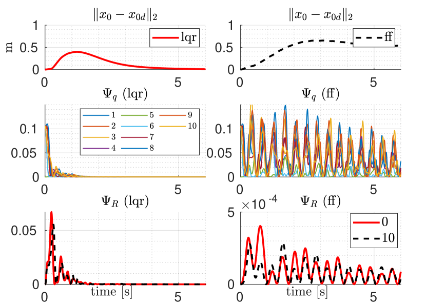
Figure 4: List of errors comparing the LQR control on the whole system (lqr) and feed-forward control on the quadrotor-position (ff). $\Psi_{q}$ is the hose link attitude errors as defined in (25) and $\Psi_{R}$ is the quadrotor attitude configuration error defined in (26).

5.1.2 (ii). Three Quadrotor system:

Setpoint tracking for cable suspended from three-quadrotors is presented here. Parameters for the system are as follows,

$$n=10,\leavevmode\nobreak\ n_{Q}=3,\leavevmode\nobreak\ \mathcal{I}=\{0,5,10\},\leavevmode\nobreak\ m_{i}=0.0909kg,\leavevmode\nobreak\ l_{i}=0.2m,$$

and $\#DOF=32,\#DOuA=20$. Various tracking errors for the system are presented in Figure 5 and snapshots for the system are shown in Figure 6.

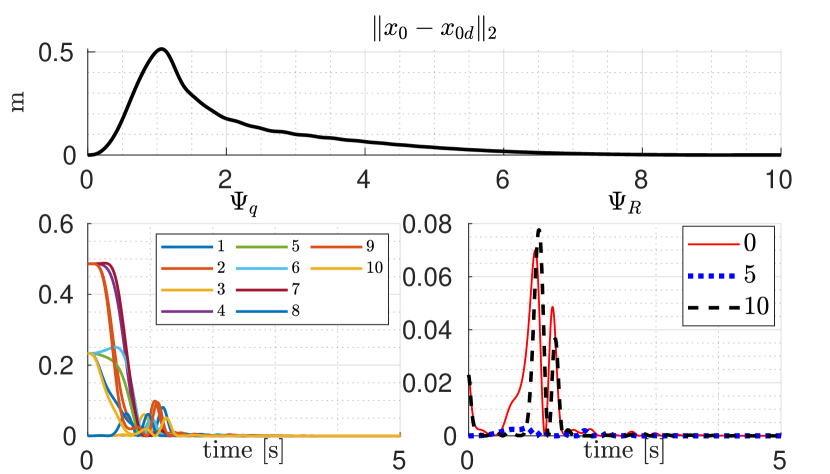
Figure 5: Tracking errors for desired set-point for $n_{Q}=3$ with the LQR control. $\Psi_{q},\Psi_{R}$ are as defined in (25)-(26).

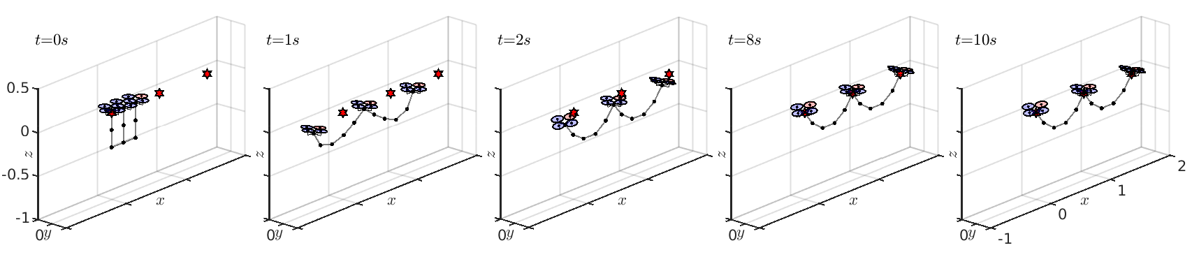
Figure 6: Snapshots of 3 quadrotor-10 link system while tracking a setpoint. Setpoints for the quadrotor position is shown by the red-hexagrams.

5.2 Trajectory Tracking

In this section, we show that the presented controller tracks a desired time-varying trajectory with initial errors. We use the following system parameters,

$$n=5,\leavevmode\nobreak\ n_{Q}=2,\mathcal{I}=\{0,5\},\leavevmode\nobreak\ m_{i}=0.1667kg,\leavevmode\nobreak\ l_{i}=0figures.2m$$

and the rest same as those given in Section 5.1. We consider the following flat output trajectory,

$$x_{0}=\begin{bmatrix}a_{x}(1{-}\cos(2f_{1}\pi t))\\ a_{y}\sin(2f_{2}\pi t)\\ a_{z}\cos(2f_{3}\pi t)\end{bmatrix},\leavevmode\nobreak\ \bar{T}_{1}=\begin{bmatrix}2.74\\ 0.0\\ -3.27\end{bmatrix},\leavevmode\nobreak\ \psi_{0}\equiv\psi_{5}\equiv 0,$$

$$f_{1}=\frac{1}{4},f_{2}=\frac{1}{5},f_{3}=\frac{1}{7},a_{x}=2,a_{y}=2.5,a_{z}=1.5.$$

Rest of the states and inputs can be computed using differential-flatness.We use the linearized-dynamics and the finite-horizon LQR presented in the previous sections to achieve the tracking control. Following weights are used for the LQR,

$$Q_{x}=0.5I_{6},\leavevmode\nobreak\ Q_{q}=0.75I_{6n},\leavevmode\nobreak\ Q_{R}=I_{3n_{Q}},Q_{\Omega}=0.75I_{3n_{Q}},$$

$$Q=bdiag(Q_{x},Q_{q},Q_{R},Q_{\Omega}),$$

$$R=0.2I_{4n_{Q}},P_{T}=0.01I_{n_{x}},$$

where $n_{x}=6{+}6n{+}6n_{Q}$. Figure 7 shows snapshots of the system at different instants along the trajectory. The proposed controller tracks the desired trajectory (shown in red) when started with an initial error.

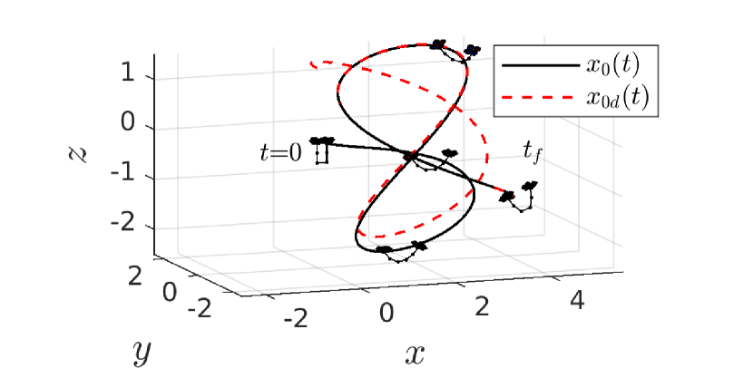
Figure 7: Snapshots of the multiple quadrotors carrying a flexible hose system while tracking the desired trajectory (shown in red) and the resulting trajectory when started with an initial error(shown in black).

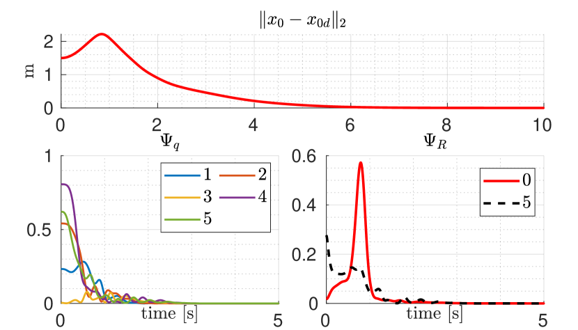
Figure 8: Errors for the trajectory tracking control shown in Fig. 7. $\Psi_{q},\Psi_{R}$ are as defined in (25)-(26).

6 Results and Discussion

Having presented numerical results to validate our controller, we now present some discussion on limitations and future work.

Limitations

Though increasing discretization helps better represent the dynamics of an hose system, it also increases the computation-complexity. To better study the effect of discretization we ran multiple simulations with different discretizations for a fixed cable length and mass. We used only control on the quadrotor-positions with feed-forward cable tensions. We used MATLAB 2018a with Intel Core $i7{-}6850\textsc{K cpu}@3.60GHz\times 12$ to run the simulations. Computation times to simulate $10s$ for different $n$ are shown in Figure 9. As illustrated in the Figure, computation time increases super-linearly with $n$.

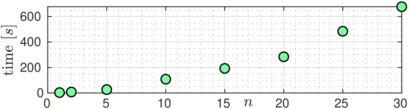
Figure 9: Computation time to simulate $10s$ for different discretizations $n$.

While differential-flatness can be used to plan trajectories in the flat-output space and compute desired states and inputs, this computation requires computing $q_{i}$ and its derivatives from tension $\vec{T}_{i}$ and its derivatives, i.e. $q_{i}=\frac{\vec{T}_{i}}{\|\vec{T}_{i}\|}$. The complexity of this computation increases for higher-derivatives.

In addition, as listed in the Section 2, we don’t consider the mechanical properties of the hose when deriving the dynamics. Thus, the dynamics derived and the subsequent presented control might not completely capture the system fully and might lead to instability in cases when hose properties are important, such as when water flows in the hose.

Future Work

As part of future work, we would like to address some of the limitations listed in the previous sections, such as, (i) number of discretizations, (ii) number of derivatives to computed, and (iii) water flow in the hose. We would like to study the current system along with all the mechanical properties of the cable and develop controllers for such systems. In addition, to implement the control we require state estimation of the cable which as shown is modeled as $(S^{2})^{n}$. Towards this end we hypothesize [Kotaru and Sreenath (2019)] can be extended to estimate the cable state. A possible method to improve the computation time would be to use limited cable states like mid-position of the cable etc., to develop a controller.

7 Conclusion

In this work we have studied the multiple quadrotors carrying a flexible hose system. We modeled the flexible-hose as a series of smaller discrete-links with lumped mass and derived the coordinate-free dynamics using Langrange-d’Alembert’s principle. We also showed that the given system is differentially-flat, as long as the end of the hose is connected to a quadrotor. Variation-based linearized dynamics were derived about time-varying desired trajectory. We showed tracking control for the system using finite-horizon LQR for the linear dynamics and validated this through numerical simulations with up-to 10 discretizations of the hose. Finally, we discussed some of the limitations due to the assumptions and directions for future work.

Appendix A Dynamics Derivation

In this section, we present the detailed derivation of the equations of motion, (4)-(6), for the given system. Starting with the principle of least action in (8) and substituting for Lagrangian and virtual work from (3),(7) and (9), we have,

$$\delta\int\Big{(}\sum_{i\in\mathcal{S}}\frac{1}{2}\overline{m}_{i}\langle v_{i},v_{i}\rangle-\overline{m}_{i}g\bm{e_{3}}\cdot x_{i}+\sum_{j\in\mathcal{I}}\underbrace{\frac{1}{2}\langle\Omega_{j},J_{j}\Omega_{j}\rangle}_{rot.energy}\Big{)}$$

$$\int\Big{(}\sum_{j\in\mathcal{I}}\underbrace{\langle W_{1j},\hat{M}_{j}\rangle}_{rot.work}+\langle W_{2j},f_{j}R_{j}\bm{e_{3}}\rangle\Big{)}dt.$$ (27)

Separating and solving the rotational components, we have the following rotational dynamics

$$J_{j}\dot{\Omega}_{j}=M-\Omega_{j}\times J_{j}\Omega_{j},\quad\forall\leavevmode\nobreak\ j\in\mathcal{I}$$ (28)

Taking variation on rest of the equation results in,

$$\int\sum_{i\in\mathcal{S}}\Bigg{[}{\overline{m}_{i}}\langle\delta v_{i},v_{i}\rangle+\delta x_{i}\cdot\underbrace{(-{\overline{m}_{i}}g\bm{e_{3}}+f_{i}R_{i}\bm{e_{3}}\mathbf{1}_{i})}_{u_{i}}\Bigg{]}dt=0.$$

Expanding the summation,

$$\bigint\begin{pmatrix}{\overline{m}_{0}}\langle\delta v_{0},v_{0}\rangle+\delta x_{0}\cdot u_{0}+\\ {\overline{m}_{1}}\langle\delta v_{1},v_{1}\rangle+\delta x_{1}\cdot u_{1}+\\ \vdots\\ {\overline{m}_{n}}\langle\delta v_{n},v_{n}\rangle+\delta x_{n}\cdot u_{n}\end{pmatrix}dt=0$$

Replacing the variations $\delta v_{i},\delta x_{i}$ with their expansions (12), (13), we get,

$$\bigint\begin{pmatrix}\big{(}{\overline{m}_{0}}\langle\delta v_{0},v_{0}\rangle+\delta x_{0}\cdot u_{0}\big{)}+\\ \big{(}{\overline{m}_{1}}\langle\delta v_{0}{-}l_{1}({q}^{\times}_{1}\dot{\xi_{1}}+{\dot{q_{1}}}^{\times}\xi_{1}),v_{1}\rangle\\ \quad\quad\quad+(\delta x_{0}{-}l_{1}{q_{1}}^{\times}\xi_{1})\cdot u_{1}\big{)}+\\ \vdots\\ \big{(}{\overline{m}_{n}}\langle\delta v_{0}{-}\sum_{k=1}^{n}l_{k}({q}^{\times}_{k}\dot{\xi_{k}}+{\dot{q_{k}}}^{\times}\xi_{k}),v_{n}\rangle\\ \quad\quad\quad+(\delta x_{0}{-}\sum_{k=1}^{n}l_{k}{q_{k}}^{\times}\xi_{k})\cdot u_{n}\big{)}\end{pmatrix}dt=0$$ (29)

Using the following simplifications in (29),

$$\langle-l_{k}({q}^{\times}_{k}\dot{\xi_{k}}+{\dot{q_{k}}}^{\times}\xi_{k}),v\rangle=l_{k}({q_{k}}^{\times}v)\cdot\dot{\xi}_{k}+l_{k}({\dot{q}_{k}}^{\times}v)\cdot\xi_{k},$$

$$-l_{k}({q_{k}}^{\times}\xi_{k})\cdot u=l_{k}({q_{k}}^{\times}u)\cdot\xi_{k},$$

and regrouping the respective variations would result in,

$$\bigint\begin{pmatrix}\delta v_{0}\cdot\sum_{k=0}^{n}\overline{m}_{k}v_{k}+\delta x_{0}\cdot\sum_{k=0}^{n}u_{k}+\\ \Big{[}\dot{\xi}_{1}\cdot\big{(}l_{1}{q_{1}}^{\times}\sum_{k=1}^{n}\overline{m}_{k}v_{k}\big{)}+\\ {\footnotesize\xi_{1}\cdot\big{(}l_{1}{\dot{q}_{1}}^{\times}\displaystyle\sum_{k=1}^{n}\overline{m}_{k}v_{k}{+}l_{1}{q_{1}}^{\times}\displaystyle\sum_{k{=}1}^{n}u_{k}\big{)}\Big{]}+}\\ \vdots\\ \Big{[}\dot{\xi}_{n}\cdot(\overline{m}_{n}l_{n}({q_{n}}^{\times}v_{n}))+\\ \xi_{n}\cdot(\overline{m}_{n}l_{n}({\dot{q}_{n}}^{\times}v)+l_{n}({q_{n}}^{\times}u_{n}))\Big{]}\end{pmatrix}dt{=}0.$$ (30)

Integration by parts on the respective variation sets results in

$$\bigint\begin{pmatrix}-\delta x_{0}\cdot(\overline{m}_{0}\dot{v}_{0}+\overline{m}_{1}\dot{v}_{1}+\ldots\overline{m}_{n}\dot{v}_{n})+\\ \delta x_{0}\cdot\big{(}\sum_{k=0}^{n}u_{k}\big{)}+\\ -{\xi}_{1}{\cdot}\bigg{(}\cancel{l_{1}{\dot{q}_{1}}^{\times}\sum_{k=1}^{n}\overline{m}_{k}v_{k}}{+}l_{1}{{q}_{1}}^{\times}\displaystyle\sum_{k=1}^{n}\overline{m}_{k}\dot{v}_{k}\bigg{)}\\ {+}\xi_{1}{\cdot}\bigg{(}\cancel{l_{1}{\dot{q}}^{\times}_{1}\displaystyle\sum_{k=1}^{n}\overline{m}_{k}v_{k}}{+}l_{1}{q}^{\times}_{1}\sum_{k=1}^{n}u_{k}\bigg{)}\\ \vdots\\ -{\xi}_{n}\cdot\bigg{(}l_{n}{{q}_{n}}^{\times}\overline{m}_{n}\dot{v}_{n}\bigg{)}+\xi_{n}\cdot\bigg{(}l_{n}{q_{n}}^{\times}u_{n}\bigg{)}\end{pmatrix}dt{=}0,$$ (31)

and finally,

$$\bigint\begin{pmatrix}\delta x_{0}\cdot\big{(}\sum_{k=0}^{n}-\overline{m}_{k}\dot{v}_{k}+u_{k}\big{)}+\\ {\xi}_{1}{\cdot}l_{1}{{q}_{1}}^{\times}\bigg{(}\sum_{k=1}^{n}-\overline{m}_{k}\dot{v}_{k}+u_{k}\bigg{)}\\ \vdots\\ {\xi}_{n}\cdot\bigg{(}-l_{n}{{q}_{n}}^{\times}\overline{m}_{n}\dot{v}_{n}+l_{n}{q_{n}}^{\times}u_{n}\bigg{)}\end{pmatrix}dt{=}0.$$ (32)

By principle of least action the above integral is valid $\forall\delta x_{0},\xi_{i},t$ and thus, to ensure the above equation to be zero for all time we have,

$$\begin{matrix}\big{(}-(\overline{m}_{0}\dot{v}_{0}+\overline{m}_{1}\dot{v}_{1}+\ldots\overline{m}_{n}\dot{v}_{n})+\sum_{k=0}^{n}u_{k}\big{)}=0\\ q_{1}{\times},\bigg{(}-l_{1}{{q}}^{\times}_{1}\sum_{k=1}^{n}\overline{m}_{k}\dot{v}_{k}+l_{1}{q}^{\times}_{1}\sum_{k=1}^{n}u_{k}\bigg{)}=0,\\ \vdots\\ q_{n}\times\bigg{(}-l_{n}{{q}_{n}}^{\times}\overline{m}_{n}\dot{v}_{n}+l_{n}{q_{n}}^{\times}u_{n}\bigg{)}=0.\end{matrix}$$ (33)

Expanding the $\dot{v}_{i}$ we have,

$$(\overline{m}_{0}\dot{v}_{0}+\overline{m}_{1}(\dot{v}_{0}+\sum_{k=1}^{1}l_{k}\ddot{q}_{k})+\ldots+\overline{m}_{n}(\dot{v}_{0}+\sum_{k=1}^{n}l_{k}\ddot{q}_{k}))=\sum_{k=0}^{n}u_{k},$$

$$l_{1}({{q}}^{\times}_{1})^{2}\big{(}\overline{m}_{1}(\dot{v}_{0}+\sum_{k=1}^{1}l_{k}\ddot{q}_{k})+\ldots\overline{m}_{n}(\dot{v}_{0}+\sum_{k=1}^{n}l_{k}\ddot{q}_{k})\big{)}{=}l_{1}({q}^{\times}_{1})^{2}\sum_{k=1}^{n}u_{k},$$

$$\vdots$$

$$l_{n}({{q}}^{\times}_{n})^{2}\big{(}\overline{m}_{n}(\dot{v}_{0}+\sum_{k=1}^{n}l_{k}\ddot{q}_{k})\big{)}=l_{n}({q}^{\times}_{n})^{2}\sum_{k=n}^{n}u_{k}.$$

Simplifying the above equations using (14) and the following relations,

$$\dot{q}=\omega{\times}q,$$

$$\ddot{q}=\dot{\omega}{\times}q+\omega{\times}\dot{q}=\dot{\omega}{\times}q-\|\omega\|^{2}q$$

$$({q}^{\times})^{2}\ddot{q}=q{\times}(q{\times}\ddot{q})=(q\cdot\ddot{q})q-(q\cdot q)\ddot{q}=-(\dot{q}\cdot\dot{q})q-\ddot{q},$$

would result in (5).

Appendix B Differential flatness

In this section, we present the proof for differential-flatness stated in Lemma 3 Illustration of the differential-flatness is shown in Figure 2. For the purpose of proving differential-flatness we redefine the dynamics of the system using tensions in the cable links as given below,

$$\overline{m}_{0}\ddot{x}_{0} =T_{1}-\overline{m}_{0}g\bm{e_{3}},$$ (34)

$$\overline{m}_{a}\ddot{x}_{a} =T_{a{+}1}-T_{a}-\overline{m}_{a}g\bm{e_{3}},$$ (35)

$$\overline{m}_{b}\ddot{x}_{b} =T_{b+1}-T_{b}-\overline{m}_{a}g\bm{e_{3}}+f_{b}R_{b}\bm{e_{3}},$$ (36)

$$\overline{m}_{b}\ddot{x}_{n} =-T_{n}-\overline{m}_{n}g\bm{e_{3}}+f_{n}R_{n}\bm{e_{3}},$$ (37)

where $\forall a\in\mathcal{S}\backslash\{0,\mathcal{I}\}$ i.e., all the points excluding the starting point of the cable and those connected to the quadrotors and $\leavevmode\nobreak\ \forall b\in\mathcal{I}\backslash\{n\}$ and the quadrotor attitude dynamics are as given in (6). Also note $n{\in}\mathcal{I}$, i.e., end the cable is attached to the quadrotor. Number of inputs in the system are $4n_{Q}$ corresponding to the thrust and moment of the quadrotors. Number of flat outputs are $3$ (for position $x_{0}$) + $3(n_{Q}-1)$ ($3\text{ for each tension }T_{k{+}1}\forall k\in\mathcal{I}\backslash\{n\})\text{ and }n_{Q}(\text{ for each quadrotor yaw }\psi_{j})=4n_{Q}$.

Making use of the these dynamics we prove the flatness as follows.

1. Given, $x_{0}$ is a flat-output and therefore we have the cable start position and its derivatives as shown,

   $$\{x_{0},\dot{x}_{0},\ddot{x}_{0},x^{(3)}_{0},\ldots,x^{(2n+4)}_{0}\}.$$ (38)

2. Taking derivatives of (34) and making use of (38) we have tension vector $T_{1}$ in the first link and its derivatives,

   $$\{T_{1},\dot{T}_{1},\ddot{T}_{1},T^{(3)}_{1}\ldots,T^{(2n+2)}_{1}\}.$$ (39)

3. Attitude of the first link is then determined from the tension vector in (39) as

   $$q_{1}=T_{1}/\|T_{1}\|$$ (40)

   and its higher derivatives,

   $$\{\dot{q}_{1},\ldots,q^{(2n+2)}_{1}\},$$ (41)

   are computed by taking derivatives of (40) and using (39).

4. Position and its derivatives of the next link point-mass $\overline{m}_{1}$ is computed using (1),

   $$\{x_{1},\dot{x}_{1},\ddot{x}_{1},\ldots,x_{1}^{(2n+2)}\}.$$ (42)

5. Repeating the steps (ii)-(iv), we can compute the link attitudes, tensions and the positions iteratively till $x_{b}$.

6. Using (36) and the fact that $T_{b+1}$ is a flat-output (note $b\in\mathcal{I}\backslash\{n\}$) we can compute the thrust in the quadrotor $f_{b}R_{b}\bm{e_{3}}$.

7. From $x_{b}$, $f_{b}R_{b}\bm{e_{3}}$ and their derivatives, the quadrotor attitude, angular velocity $R_{j},\Omega_{j}$ and moment $M_{j}$ can be computed as shown in [Mellinger and Kumar (2011)].

8. Rest of the states and inputs for the multiple quadrotors carrying a flexible hose segments can be iteratively determined as described above.

Proof for Corollary 1 is given below, For tethered system we have $x_{0}\equiv 0$ and $T_{1}$ is known since it-is a flat-output, i.e., steps (i)-(ii) (see (38)-(39)). Rest of the proof follows form Lemma 3.

Appendix C Variation-based Linearized Dynamics

Taking variations with respect to desired states for various states is as follows,

$$\delta q_{i}={\xi}^{\times}_{i}q_{id}=-{q}^{\times}_{id}\xi_{i}$$ (43)

$$\delta(\|\omega_{i}\|^{2})=\delta(\omega_{i}^{\top}\omega_{i})=2\omega_{id}^{\top}(\delta\omega_{i})$$ (44)

$$\delta R_{j}=R_{jd}{\eta}^{\times}_{j}$$ (45)

Taking variation on the first row of (5),

$$\delta\Bigg{(}M_{00}I_{3}\dot{v}_{0}-\sum_{i=1}^{n}M_{0i}{q}^{\times}_{i}\dot{\omega}_{i}=\sum_{i=1}^{n}M_{0i}\|\omega_{i}\|^{2}q_{i}+\sum_{k=0}^{n}u_{k}\Bigg{)}$$ (46)

$$M_{00}I_{3}\delta\dot{v}_{0}-\sum_{i=1}^{n}M_{0i}{q}^{\times}_{id}\delta\dot{\omega}_{i}=$$

$$\sum_{i=1}^{n}\Big{(}M_{0i}\big{[}({\dot{\omega}}^{\times}_{id}-\|\omega_{id}\|^{2}I_{3}){q}^{\times}_{id}\big{]}\xi_{i}+M_{0i}(2q_{id}\omega_{id}^{\top})\delta\omega_{i}\Big{)}$$

$$+\sum_{k=0}^{n}\big{(}(\delta f_{k})R_{kd}e_{3}\mathbf{1}_{k}+f_{kd}\delta R_{kd}e_{3}\mathbf{1}_{k}\big{)}$$ (47)

taking variation on rest of the equations,

$${\delta\Big{(}}M_{i0}{q}^{\times}_{i}\dot{v}_{0}+M_{ii}I_{3}\dot{\omega}_{i}-\sum_{j=1,j\neq i}^{n}M_{ij}{q}^{\times}_{i}{q}^{\times}_{j}\dot{\omega}_{j}=$$

$$\sum_{k=1}^{n}(M_{ik}\|\omega_{k}\|^{2}{q}^{\times}_{i}q_{k})+l_{i}({q}^{\times}_{i})\sum_{k=i}^{n}u_{k}{\Big{)}}$$ (48)

$$M_{i0}\big{(}\delta({q}^{\times}_{i})\dot{v}_{0d}+{q}^{\times}_{id}\delta\dot{v}_{0}\big{)}+M_{ii}I_{3}\delta\dot{\omega}_{i}$$

$$-\sum_{j=1,j\neq i}^{n}M_{ij}\big{[}\delta({q}^{\times}_{i}){q}^{\times}_{jd}\dot{\omega}_{jd}+{q}^{\times}_{id}\delta({q}^{\times}_{j})\dot{\omega}_{jd}+{q}^{\times}_{id}{q}^{\times}_{jd}\delta\dot{\omega}_{j}\big{]}$$

$$=\sum_{k=1}^{n}(M_{ik}\big{[}2{q}^{\times}_{id}q_{kd}\omega^{\top}_{kd}\delta\omega_{k}+\|\omega_{kd}\|^{2}\delta({q}^{\times}_{i})q_{kd}+$$

$$\|\omega_{k}\|^{2}{q}^{\times}_{i}\delta{q_{kd}}\big{]})+l_{i}\delta({q}^{\times}_{i})\sum_{k=i}^{n}u_{k}+l_{i}({q}^{\times}_{i})\sum_{k=i}^{n}\delta u_{k}$$ (49)

$$M_{i0}{q}^{\times}_{id}\delta\dot{v}_{0}+M_{ii}I_{3}\delta\dot{\omega}_{i}-\sum_{j=1,j\neq i}^{n}M_{ij}\big{[}{q}^{\times}_{id}{q}^{\times}_{jd}\delta\dot{\omega}_{j}\big{]}$$

$$=\Big{[}M_{io}{\dot{v}_{0d}}^{\times}-\sum_{j=1,j\neq i}^{n}M_{ij}\big{(}{({q}^{\times}_{jd})\dot{\omega}_{jd})}^{\times}+\|\omega_{jd}\|^{2}{q}^{\times}_{jd}\big{)}-l_{i}{\big{(}\sum_{k=i}^{n}{u}^{\times}_{k}\big{)}}\Big{]}(-{q}^{\times}_{i}){\xi}_{i}$$

$$+\sum_{j=1,j\neq i}^{n}\Big{[}M_{ij}{q}^{\times}_{id}\big{(}{\dot{\omega}}^{\times}_{jd}-\|\omega_{jd}\|^{2}I\big{)}{q}^{\times}_{jd}\Big{]}\xi_{j}+\sum_{j=1,j\neq i}^{n}M_{ij}\big{[}2{q}^{\times}_{id}q_{jd}\omega^{\top}_{jd}\big{]}\delta\omega_{j}$$

$$+l_{i}({q}^{\times}_{i})\sum_{k=i}^{n}((\delta f_{k})R_{kd}e_{3}\mathbf{1}_{k}+f_{kd}\delta R_{kd}e_{3}\mathbf{1}_{k})$$ (50)

$$M_{00}I_{3}\delta\dot{v}_{0}-\sum_{i=1}^{n}M_{0i}{q}^{\times}_{id}\delta\dot{\omega}_{i}=$$

$$\sum_{i=1}^{n}\Big{(}M_{0i}\big{[}({\dot{\omega}}^{\times}_{id}-\|\omega_{id}\|^{2}I_{3}){q}^{\times}_{id}\big{]}\xi_{i}+M_{0i}(2q_{id}\omega_{id}^{\top})\delta\omega_{i}\Big{)}+$$

$$\sum_{k{\in}\mathcal{I}}\big{(}(\delta f_{k})R_{kd}e_{3}+f_{kd}\delta R_{kd}e_{3}\big{)}$$ (51)

$$M_{i0}{q}^{\times}_{id}\delta\dot{v}_{0}+M_{ii}I_{3}\delta\dot{\omega}_{i}-\sum_{j=1,j\neq i}^{n}M_{ij}\big{[}{q}^{\times}_{id}{q}^{\times}_{jd}\delta\dot{\omega}_{j}\big{]}$$

$$=\Big{[}M_{io}{\dot{v}_{0d}}^{\times}-\sum_{j=1,j\neq i}^{n}M_{ij}\big{(}{({q}^{\times}_{jd})\dot{\omega}_{jd})}^{\times}+\|\omega_{jd}\|^{2}{q}^{\times}_{jd}\big{)}-l_{i}{\big{(}\sum_{k=i}^{n}{u}^{\times}_{k}\big{)}}\Big{]}(-{q}^{\times}_{i}){\xi}_{i}$$

$$+\sum_{j=1,j\neq i}^{n}\Big{[}M_{ij}{q}^{\times}_{id}\big{(}{\dot{\omega}}^{\times}_{jd}-\|\omega_{jd}\|^{2}I\big{)}{q}^{\times}_{jd}\Big{]}\xi_{j}+\sum_{j=1,j\neq i}^{n}M_{ij}\big{[}2{q}^{\times}_{id}q_{jd}\omega^{\top}_{jd}\big{]}\delta\omega_{j}$$

$$+l_{i}({q}^{\times}_{i})\sum_{k=i}^{n}((\delta f_{k})R_{kd}e_{3}\mathbf{1}_{k}+f_{kd}\delta R_{kd}e_{3}\mathbf{1}_{k})$$ (52)

From (47) & (52), we have,

$$\begin{bmatrix}M_{00}I_{3}&-{q}^{\times}_{1d}M_{01}&-{q}^{\times}_{2d}M_{02}&\ldots&-{q}^{\times}_{nd}M_{0n}\\[8.61108pt] M_{10}{q}^{\times}_{1}&M_{11}I_{3}&-M_{12}{q}^{\times}_{1d}{q}^{\times}_{2d}&\ldots&-M_{1n}{q}^{\times}_{1d}{q}^{\times}_{nd}\\[8.61108pt] M_{20}{q}^{\times}_{2d}&-M_{21}{q}^{\times}_{2d}{q}^{\times}_{1d}&M_{22}I_{3}&\ldots&-M_{2n}{q}^{\times}_{2d}{q}^{\times}_{nd}\\[8.61108pt] \vdots&\vdots&\vdots&\ddots&\vdots\\[8.61108pt] M_{n0}{q}^{\times}_{nd}&-M_{n1}{q}^{\times}_{nd}{q}^{\times}_{1d}&-M_{n2}{q}^{\times}_{nd}{q}^{\times}_{2d}&\ldots&M_{nn}I_{3}\end{bmatrix}\begin{bmatrix}\delta v_{0}\\ \delta\dot{\omega}_{1}\\ \vdots\\ \delta\dot{\omega}_{n}\end{bmatrix}$$

$$\setcounter{MaxMatrixCols}{14}\begin{bmatrix}O&a_{1}&\ldots&a_{n}&O&b_{1}&\ldots&b_{n}&e_{1}&\ldots&e_{n_{Q}}&O&\ldots&O\\ O&c_{11}&\ldots&c_{1n}&O&d_{11}&\ldots&d_{1n}&f_{11}&&f_{1n_{Q}}&O&\ldots&O\\ \vdots&\vdots&\ddots&\vdots&\vdots&\vdots&\ddots&\vdots&&\ddots&&\vdots&\ddots&\vdots\\ O&c_{n1}&\ldots&c_{nn}&O&d_{n1}&\ldots&d_{nn}&&&f_{n_{Q}n_{Q}}&O&\ldots&O\end{bmatrix}\begin{bmatrix}\delta x\\ \xi_{1}\\ \vdots\\ \xi_{n}\\ \delta v\\ \delta\omega_{1}\\ \vdots\\ \delta\omega_{n}\\ \eta_{j1}\\ \vdots\\ \eta_{jn_{Q}}\\ \delta\Omega_{j1}\\ \vdots\\ \delta\Omega_{jn_{Q}}\end{bmatrix}+G\delta\mathbf{u},$$ (53)

where

$$a_{i} =M_{0i}\big{[}({\dot{\omega}}^{\times}_{id}-\|\omega_{id}\|^{2}I_{3}){q}^{\times}_{id}$$ (54)

$$b_{i} =M_{0i}(2q_{id}\omega_{id}^{\top}),\quad i=\{1,\ldots,n\}$$ (55)

$$c_{ij} =\begin{cases}\big{[}M_{io}{\dot{v}_{0d}}^{\times}-\sum_{j=1,j\neq i}^{n}M_{ij}\big{(}{({q}^{\times}_{jd})\dot{\omega}_{jd})}^{\times}+\|\omega_{jd}\|^{2}{q}^{\times}_{jd}\big{)}-l_{i}{\big{(}\sum_{k=i}^{n}{u}^{\times}_{k}\big{)}}\big{]}(-{q}^{\times}_{i})&\quad i=j\\ \big{[}M_{ij}{q}^{\times}_{id}\big{(}{\dot{\omega}}^{\times}_{jd}-\|\omega_{jd}\|^{2}I\big{)}{q}^{\times}_{jd}\big{]}&\quad i\neq j\end{cases}$$ (56)

$$d_{ij} =\begin{cases}O&\quad i=j\\ M_{ij}\big{[}2{q}^{\times}_{id}q_{jd}\omega^{\top}_{jd}\big{]}&\quad i\neq j\end{cases}$$ (57)

$$e_{j} =-f_{jd}R_{jd}{e}^{\times}_{3},\quad j\in{\mathcal{I}}$$ (58)

$$f_{ij} =\begin{cases}[]&if\leavevmode\nobreak\ j\notin\mathcal{I}\\ -(l_{i}{q}^{\times}_{i})f_{jd}R_{jd}{e_{3}}^{\times},&if\leavevmode\nobreak\ j\in\mathcal{I},j\geq i\\ O_{3,3}&if\leavevmode\nobreak\ j\in\mathcal{I},j<i\end{cases}$$ (59)

$$g_{j} =R_{jd}e_{3}$$ (60)

$$h_{ij} =\begin{cases}[]&if\leavevmode\nobreak\ j\notin\mathcal{I}\\ (l_{i}{q}^{\times}_{i})R_{jd}{e_{3}},&if\leavevmode\nobreak\ j\in\mathcal{I},j\geq i\\ O_{3,1}&if\leavevmode\nobreak\ j\in\mathcal{I},j<i\end{cases}$$ (61)

References

• Aerones (2018) Aerones (2018). Firefighting drone. URL https://www.aerones.com/eng/firefighting_drone/.
• Bernard et al. (2011) Bernard, M., Kondak, K., Maza, I., and Ollero, A. (2011). Autonomous transportation and deployment with aerial robots for search and rescue missions. Journal of Field Robotics, 28(6), 914–931.
• Goodarzi et al. (2014) Goodarzi, F.A., Lee, D., and Lee, T. (2014). Geometric stabilization of a quadrotor uav with a payload connected by flexible cable. In American Control Conference, 4925–4930.
• Goodarzi et al. (2015) Goodarzi, F.A., Lee, D., and Lee, T. (2015). Geometric control of a quadrotor uav transporting a payload connected via flexible cable. International Journal of Control, Automation and Systems, 13(6), 1486–1498.
• Goodarzi and Lee (2015) Goodarzi, F.A. and Lee, T. (2015). Dynamics and control of quadrotor uavs transporting a rigid body connected via flexible cables. In American Control Conference, 4677–4682.
• Goodarzi and Lee (2016) Goodarzi, F.A. and Lee, T. (2016). Stabilization of a rigid body payload with multiple cooperative quadrotors. Journal of Dynamic Systems, Measurement, and Control, 138(12), 121001.
• Jiang and Kumar (2012) Jiang, Q. and Kumar, V. (2012). The inverse kinematics of cooperative transport with multiple aerial robots. IEEE Transactions on Robotics, 29(1), 136–145.
• Kotaru and Sreenath (2019) Kotaru, P. and Sreenath, K. (2019). Variation based extended kalman filter on $s^{2}$. In European Control Conference (ECC), 875–882.
• Kotaru et al. (2018) Kotaru, P., Wu, G., and Sreenath, K. (2018). Differential-flatness and control of quadrotor (s) with a payload suspended through flexible cable (s). In Indian Control Conference (ICC), 352–357.
• Lee and Kim (2017) Lee, H. and Kim, H.J. (2017). Constraint-based cooperative control of multiple aerial manipulators for handling an unknown payload. IEEE Transactions on Industrial Informatics, 13(6), 2780–2790.
• Lee (2015) Lee, T. (2015). Geometric controls for a tethered quadrotor uav. In Conference on Decision and Control (CDC), 2749–2754.
• Lee et al. (2013) Lee, T., Sreenath, K., and Kumar, V. (2013). Geometric control of cooperating multiple quadrotor uavs with a suspended payload. In Conference on decision and control, 5510–5515.
• Liu et al. (2017) Liu, Z., Liu, J., and He, W. (2017). Modeling and vibration control of a flexible aerial refueling hose with variable lengths and input constraint. Automatica, 77, 302–310.
• Lupashin and D’Andrea (2013) Lupashin, S. and D’Andrea, R. (2013). Stabilization of a flying vehicle on a taut tether using inertial sensing. In 2013 IEEE/RSJ International Conference on Intelligent Robots and Systems, 2432–2438.
• Maza et al. (2009) Maza, I., Kondak, K., Bernard, M., and Ollero, A. (2009). Multi-uav cooperation and control for load transportation and deployment. In International Symposium on UAVs, Reno, Nevada, USA June 8–10, 2009, 417–449. Springer.
• Mellinger and Kumar (2011) Mellinger, D. and Kumar, V. (2011). Minimum snap trajectory generation and control for quadrotors. In 2011 IEEE International Conference on Robotics and Automation, 2520–2525.
• Mellinger et al. (2013) Mellinger, D., Shomin, M., Michael, N., and Kumar, V. (2013). Cooperative grasping and transport using multiple quadrotors. In Distributed autonomous robotic systems, 545–558. Springer.
• Merino et al. (2012) Merino, L., Caballero, F., Martínez-De-Dios, J.R., Maza, I., and Ollero, A. (2012). An unmanned aircraft system for automatic forest fire monitoring and measurement. Journal of Intelligent & Robotic Systems, 65(1-4), 533–548.
• Michael et al. (2011) Michael, N., Fink, J., and Kumar, V. (2011). Cooperative manipulation and transportation with aerial robots. Autonomous Robots, 30(1), 73–86.
• Murray et al. (1995) Murray, R.M., Rathinam, M., and Sluis, W. (1995). Differential flatness of mechanical control systems: A catalog of prototype systems. In ASME international mechanical engineering congress and exposition. Citeseer.
• Nicotra et al. (2014) Nicotra, M.M., Naldi, R., and Garone, E. (2014). Taut cable control of a tethered uav. IFAC Proceedings Volumes, 47(3), 3190–3195.
• Palunko et al. (2012) Palunko, I., Cruz, P., and Fierro, R. (2012). Agile load transportation: Safe and efficient load manipulation with aerial robots. IEEE robotics & automation magazine, 19(3), 69–79.
• PrimeAir (2019) PrimeAir, A. (2019). URL https://www.amazon.com/Amazon-Prime-Air/b?ie=UTF8&node=8037720011.
• Ro and Kamman (2010) Ro, K. and Kamman, J.W. (2010). Modeling and simulation of hose-paradrogue aerial refueling systems. Journal of guidance, control, and dynamics, 33(1), 53–63.
• SkyScopes (2017) SkyScopes (2017). Sharper shape and skyskopes pull power lines. URL https://www.skyskopes.com/post/sharper-shape-and-skyskopes-pull-power-lines.
• Sreenath and Kumar (2013) Sreenath, K. and Kumar, V. (2013). Dynamics, control and planning for cooperative manipulation of payloads suspended by cables from multiple quadrotor robots. In Robotics: Science and Systems (RSS).
• Sreenath et al. (2013) Sreenath, K., Lee, T., and Kumar, V. (2013). Geometric control and differential flatness of a quadrotor uav with a cable-suspended load. In Conference on Decision and Control, 2269–2274.
• Tognon and Franchi (2015) Tognon, M. and Franchi, A. (2015). Nonlinear observer-based tracking control of link stress and elevation for a tethered aerial robot using inertial-only measurements. In International Conference on Robotics and Automation (ICRA), 3994–3999.
• Williams and Trivailo (2007) Williams, P. and Trivailo, P. (2007). Dynamics of circularly towed aerial cable systems, part i: optimal configurations and their stability. Journal of guidance, control, and dynamics, 30(3), 753–765.
• Wu and Sreenath (2014) Wu, G. and Sreenath, K. (2014). Geometric control of multiple quadrotors transporting a rigid-body load. In Conference on Decision and Control, 6141–6148.
• Wu and Sreenath (2015) Wu, G. and Sreenath, K. (2015). Variation-based linearization of nonlinear systems evolving on $so(3)$ and $s^{2}$. IEEE Access, 3, 1592–1604.
• X-Wing (2019) X-Wing (2019). URL https://x.company/projects/wing/.