High-resolution spectroscopy of the high velocity hot post-AGB star IRAS 18379–1707 (LS 5112)

Abstract

The high-resolution ($R\sim 48\,000$) optical spectrum of the B-type supergiant LS 5112, identified as the optical counterpart of the post-AGB candidate IRAS 18379–1707 is analysed. We report the detailed identifications of the observed absorption and emission features in the wavelength range 3700-9200 Å for the first time. The absorption line spectrum has been analysed using non-LTE model atmosphere techniques to determine stellar atmospheric parameters and chemical composition. We estimate $T_{\text{eff}}=18~{}000\pm 1000$ K, $\log g=2.25\pm 0.08$, $\xi_{\rm t}=10\pm 4$  km s^-1 and $v\sin i=37\pm 6$  km s^-1, and the derived abundances indicate a metal-deficient ([M/H]$\approx-0.6)$ post-AGB star. Chemical abundances of eight different elements were obtained. The estimates of the CNO abundances in IRAS 18379–1707 indicate that these elements are overabundant with [(C+N+O)/S]=+0.5$\pm$0.2 suggesting that the products of helium burning have been brought to the surface as a result of third dredge-up on the AGB. From the absorption lines, we derived heliocentric radial velocity of $V_{\text{r}}=-124.0\pm 0.4$  km s^-1. We have identified permitted emission lines of O i, N i, Na i, S ii, Si ii, C ii, Mg ii and Fe iii. The nebula forbidden lines of [N i], [O i], [Fe ii], [N ii], [S ii], [Ni ii] and [Cr ii] have also been identified. The Balmer lines H$\alpha$, H$\beta$ and H$\gamma$ show P-Cygni behaviour clearly indicating post-AGB mass-loss process in the object with the wind velocity up to 170  km s^-1.

1 INTRODUCTION

Low- and intermediate-mass stars ($M_{\text{ZAMS}}\sim 0.8-\textendash 8M_{\odot}$) evolving from the asymptotic giant branch (AGB) to become planetary nebulae (PNe) pass through a short lived but important evolutionary stage that is designated as post-asymptotic giant branch (post-AGB). Among post-AGB stars, there is a small group of hot objects, early B supergiants with emission lines in the spectrum, that are presumed to be the immediate progenitors of the central stars of planetary nebulae (CSPN). The temperatures of these stars are already high enough for the ionization of their surrounding envelopes to begin, but the ultraviolet radiation is still insufficient for the excitation of [O iii] lines typical of PNe.

The star LS 5112 from the Catalog of Luminous stars in the Southern Milky Way by (1971) was identified with the infrared (IR) source IRAS 18379–1707 from catalogue of new possible planetary nebulae (Preite-Martinez, 1988) and was classified as a hot post-AGB star by (2000) with a spectral type of B1IIIpe and IRAS colours typical of PNe. The star is contained in The Toruń catalogue of Galactic post-AGB and related objects of (2007). Nyman et al. (1992) did not find circumstellar CO(1-2) for IRAS 18379–1707. The object is not detected in the radio at 3.6 cm (, 2004). Combining the optical, near and far-IR (ISO, IRAS) data of IRAS 18379–1707 (2004) have reconstructed its spectral energy distribution (SED) and estimated the star and dust temperatures, mass loss rates, angular radii of the inner boundary of the dust envelopes and the distances to the star. For IRAS 18379–1707 Cerrigone et al. (2009) detected a dual-chemistry circumstellar envelope, associated with the 10 $\mu$m feature and silicate features due to PAHs. These authors also present a DUSTY model of the continuum and SED and derived a stellar temperature. IRAS 18379–1707 is H ₂-emitting object. For the first time H ₂ emission from IRAS 18379–1707 is detected by Hrivnak et al. (2004). (2005) assumed that H ₂ is excited by a mixture of radiative and collisional excitation. The detailed structure of the H ₂ nebula was shown by (2015). The H ₂ nebula takes the form of an oval shell of dimensions 3.6$\times$2.2 arcsec, whereas Br $\gamma$ and He i emission is centrally located and spatially unresolved, indicating a still-compact ionized region with densities $n_{H}\sim 10^{5}$ cm³ (, 2015).

Some stellar and dust parameters of IRAS 18379–1707 are summarized in Table 1.

So far only low-resolution optical spectroscopy was performed for IRAS 18379–1707. In this paper we report an analysis of the high-resolution spectrum, on the basis of which the chemical composition was obtained for the first time and the fundamental parameters of the star with the best accuracy at the moment were determined. Because of the high-resolution spectrum we could resolve, identify and analyse many absorption lines, emission lines, and P-Cygni profiles, etc. Because of the high spectral resolution we could measure the radial velocities accurately and discovered that LS 5112 is a high velocity star.

The paper is organized as follows: in Sect. 2 we describe the observations and the data reduction; in Sect. 3 we present an analysis of the main spectral features; the estimation of atmospheric parameters and abundances are presented in Sect. 4. In Sect. 5 we analyze the emission spectrum and discuss our results in the context of post-AGB evolution in Sect. 6. In Sect. 7, we give conclusions.

Table 1: Stellar and Dust Parameters of IRAS 18379–1707.

Quantity	Value	References
Position (J2000.0)	$\alpha$=18:40:48.62 $\delta$=–17:04:38.33	SIMBAD
Gal. coord.	$l$=016.50 $b$=–05.42	SIMBAD
Parallaxes (mas)	0.2593$\pm$0.0648	G18
Distance (kpc)	3497${}_{-703}^{+1120}$	BJ18
Spectral type	OB+e, B2.5Ia, B1IIIpe	SS71, V98, P00
$T_{\text{eff}}$ (K)	19 000, 24 000	GP04, C09
$\log g$	$2.5\pm 0.5$	GP03
Magnitude	14.980(FUV) 14.599(NUV)	B-AGdC16
	11.94($U$) 12.38($B$) 11.93($V$)	R98
	10.76($J$) 10.55($H$) 10.33($K$)	GL97
	10.661($J$) 10.433($H$) 10.155($K_{s}$)	2MASS
$E(B-V)$ (mag)	0.71	GP04
$T_{\text{dust}}$ (K)	140	GP04
	120, 590	C09

References. SIMBAD: http://simbad.u-strasbg.fr/simbad/; G18: (2018); BJ: Bailer-Jones et al. (2018); SS71: (1971); V98: (1998); P00: (2000); GP04: (2004); C09: Cerrigone et al. (2009); GP03: (2003); B-AGdC16: Beitia-Antero & Gómez de Castro (2016); R98: (1998); GL97: García-Lario et al. (1997a)

2 OBSERVATIONS AND DATA REDUCTION

Two high-resolution optical spectra of IRAS 18379–1707 were acquired on April 17, 2006 with the Fiber-fed Extended Range Optical Spectrograph (FEROS) (, 1999), attached to the MPG/ESO 2.2-m telescope at La Silla Observatory, Chile (Prop.ID: 77.D-0478A, PI: M. Parthasarathy). FEROS is a bench-mounted echelle spectrograph, which provides data with a resolving power $R\sim 48\,000$ and a spectral coverage from from 3600 to 9200 Å in 39 orders. An EEV 2k$\times$4k CCD detector with a pixel size of 15 $\mu$m was used. The exposure time of each spectrum was 2700 s. The a signal-to-noise (S/N) ratio was 100 per pixel in the 5500 Å region. The reduction process was performed using the FEROS standard on-line reduction pipeline and the echelle spectra reduction package ECHELLE in IRAF using a standard reduction manner including bias subtraction, removing scattered light, detector sensitivity correction, removing cosmic-ray hits, airmass extinction correction, flux-density calibration, and an all echelle order connection. Both reduced spectra were continuum normalised, co-added and cleaned of telluric lines with MOLECFIT (, 2015).

3 DESCRIPTION OF THE HIGH RESOLUTION SPECTRUM

The optical spectrum of IRAS 18379–1707 displays stellar absorption lines, nebular emission lines and interstellar absorption features. The identification of the emission lines in spectrum of IRAS 18379–1707 are based on the Moore multiplet table (Moore, 1945) and the National Institute of Standards and Technology (NIST) Atomic Spectra Database.

The complete continuum-normalised spectrum of IRAS 18379–1707 in the spectral ranges 3700–9200 Å is presented at http://lnfm1.sai.msu.ru/~davnv/ls5112.

3.1 Photospheric absorption lines

Absorption lines of neutral species including H i, He i, C i, N i, O i and Ne i were identified. Singly-ionized species including C ii, N ii, O ii, Si ii, S ii and Mg ii were detected. Higher ionization is seen in Al iii, Si iii, S iii, and Si iv.

3.2 Nebular emission lines

The list of emission lines in IRAS 18379–1707 is given in Table LABEL:emlines. It includes the measured and laboratory wavelength (in the air), the equivalent width ($EW$), the heliocentric radial velocity ($V_{\text{r}}$), the name of the element and the multiplet number to which the measured line belongs. The hydrogen and helium lines are not included in the Table LABEL:emlines because they have the complex multicomponent profiles and will be discussed separately.

The permitted emission lines, in addition to hydrogen and helium, belong to the ions of Si ii, S ii, C ii, Mg ii and also to the nonionised atoms of O i, N i and Na i. Two weak emission lines of Fe iii $\lambda$5126 and $\lambda$5156 are also present in the spectrum of IRAS 18379–1707. In the red spectral region, the permitted O i $\lambda$8446 triplet is the most remarkable emission feature. The strong emissivity of this line as a fluorescence effect to the practically exact coincidence between L$\beta$ ($\lambda$1025) and O i line at $\lambda$1026 was explained by Bowen (1947).

The forbidden emission lines are from [Fe ii], [Ni ii], [N ii] $\lambda$6548, 6584, [S ii] $\lambda$6717, 6731, [Cr ii] as well as and [O i] $\lambda$5577, 6300, 6363. The presence of the [N ii] and [S ii] emissions indicates the onset of the ionization of the circumstellar envelope and it is evolving towards the early stage of young low excitation planetary nebula.

3.3 The hydrogen lines

Balmer lines from H 15 to H 9 consist of the photospheric absorption component and blue-shifted wind absorption. H $\epsilon$ are blended with the interstellar line of Ca ii at 3968 Å. Pashen lines on our spectrum are presented by high members from P10 and more. The line profile of each of them consist of the photospheric absorption component and weak emission on the blue wing of the absorption line.

The profiles of the first Balmer lines H$\alpha$–H$\delta$ display a complex P-Cygni structure with its blue edge reaching a value of up to –170  km s^-1. Fig. 1 shows the high-resolution spectra of the H$\alpha$, H$\beta$ and H$\gamma$. The equivalent widths of the H$\alpha$ and H$\beta$ emission component are 8.84 Å and 1.61 Å, respectively.

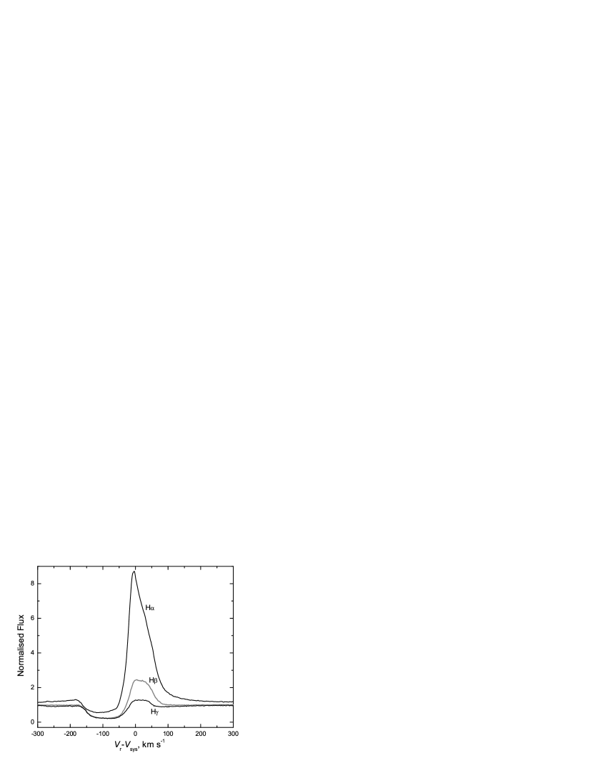
Figure 1: P-Cygni profiles of H$\alpha$, H$\beta$ and H$\gamma$ lines seen in the spectrum of IRAS 18379–1707 on a velocity scale relative to $V_{\rm sys}=-124$  km s^-1.

3.4 The helium lines

The He i emission lines in IRAS 18379–1707 are superposed on the corresponding absorption components. Fig. 2 shows the profiles of selected He i lines and compared to model spectra (see below). The asymmetric nature of the emission lines suggests that they may have P-Cygni profiles.

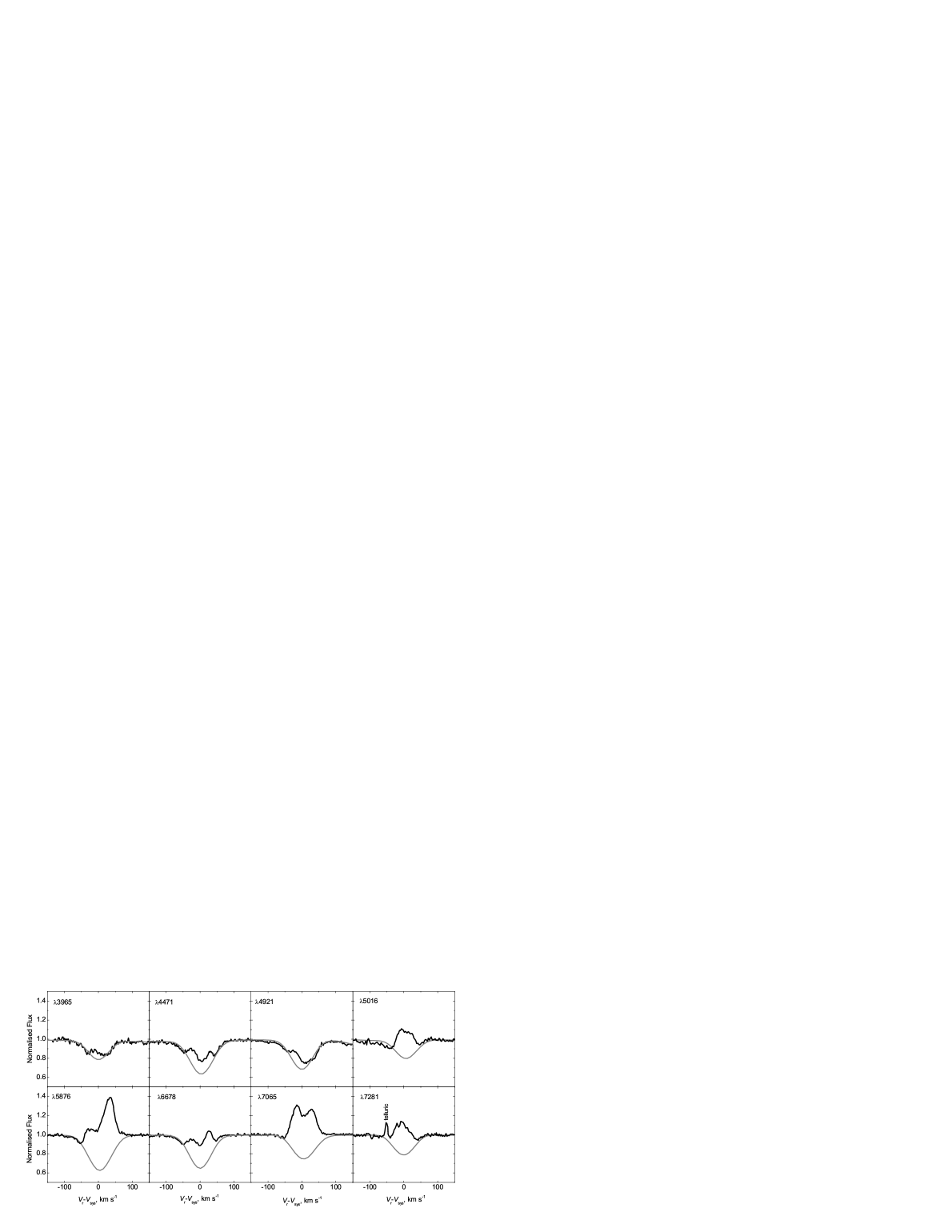
Figure 2: The profiles of selected He i lines seen in the spectrum of IRAS 18379–1707 on a velocity scale relative to $V_{\rm sys}=-124$  km s^-1and compared to model spectra (grey lines).

3.5 Interstellar features and colour excess

The spectrum of IRAS 18379–1707 contains absorption features that have interstellar origin. There are Na i doublet ($\lambda$5889.951, 5895.924), Ca ii H and K lines ($\lambda$3968.469, 3933.663), K i lines ($\lambda$7664.899, 7698.974), and Ca i at 4226.73 Å. The Na i, Ca ii and Ca i lines have multi-component profiles, whereas the K i lines show a single and sharp profiles. H line of Ca ii is very much blended with the strong stellar H $\epsilon$ feature. The selected interstellar spectral lines are depicted in Fig. 3. Heliocentric radial velocities ($V_{\text{r}}$) for the defined absorption components of Na i D1 and D2, Ca ii H and K lines are presented in Table 2. The radial velocity of the K i lines is close to the radial velocity of ‘1’ component of the Na i, Ca ii and Ca i lines and is equal to –7.9$\pm$0.5  km s^-1. If one compares the radial velocities of these components with the average radial velocities for the star –124  km s^-1(Sec. 4.1), we may infer that all components in the velocity interval from –10 to 100  km s^-1 originate in the interstellar medium. Smoker et al. (2004) found in the Ca ii K and Ca ii H spectra of IRAS 18379–1707 an absorption feature at $V_{\text{LSR}}\sim-137$  km s^-1. This component is also present in our spectrum and it is most likely of interstellar origin.

Figure 3: The profiles of the interstellar lines in the spectrum of IRAS 18379–1707. The various absorption components have been labelled.

Table 2: Absorption components of Na i D1 and D2, Ca ii H and K lines in the spectrum of IRAS 18379-1707. $V_{\text{r}}$ are the respective heliocentric radial velocities.

component	Na i D2		Na i D1		Ca ii H		Ca ii K
	$\lambda_{\text{obs.}}$	$V_{\text{r}}$	$\lambda_{\text{obs.}}$	$V_{\text{r}}$	$\lambda_{\text{obs.}}$	$V_{\text{r}}$	$\lambda_{\text{obs.}}$	$V_{\text{r}}$
	Å	km s-1	Å	km s-1	Å	km s-1	Å	km s-1
1	5889.75	–10.33	5895.73	–9.81	3968.36	–7.86	3933.57	–7.04
2	5890.41	23.26	5896.41	24.76	3968.78	24.26	3933.98	24.19
3	5890.71	38.53	5896.71	40.02	–	–	–	–
4	5891.16	61.44	5897.13	61.37	3969.27	60.30	3934.45	60.16
5	5891.91	99.61	5897.88	99.51	3969.75	96.73	3934.95	97.68

In addition to the above-mentioned interstellar atomic lines, our echelle spectra contain several quite strong Diffuse Interstellar Bands (DIBs) presented in Table 3. It includes the measured wavelength and the central wavelength from (2008), the width (FWHM), the equivalent width ($EW$), $EW/E(B-V)$ from Luna et al. (2008), $E(B-V)$ and the radial velocity ($V_{\text{r}}$). Three of DIBs centred at 6284, 6993, and 7224 Å are strongly affected by telluric contamination. For these features, the telluric component was removed before determining their parameters.

As seen in Table 3 the radial velocities of most DIBs are close to those of ‘1’ or ‘2’ components of the Na i, Ca ii interstellar lines. A radial velocity analysis of the DIBs observed in IRAS 18379–1707 confirms our result, as the Doppler shifts measured are found to be consistent with an interstellar origin.

Using $EW/E(B-V)$ from Luna et al. (2008) we estimated the extinction by 8 DIBs and obtained the mean value $E(B-V)=0.61\pm 0.08$ mag. The DIB at 5849.81 Å which is found to be unusually strong was excluded from the consideration. The resulting $E(B-V)$ value is close to the $E(B-V)=0.71$ mag obtained by (2003, 2004).

An analysis of DIBs observed in IRAS 18379–1707 confirms the conclusion of Luna et al. (2008) that, like in other post-AGB stars, these features are of exclusively interstellar origin.

Table 3: DIBs in the spectrum of IRAS 18379–1707.

$\lambda_{\text{obs.}}$	$\lambda_{\text{c}}$	FWHM	$EW$	$\frac{EW}{E(B-V)}$	$E(B-V)$	$V_{\text{r}}$
Å	Å	Å	Å	Å/mag	mag	km s-1
4963.72	4963.88	0.62	0.02	–	–	-9.7
5488.10	5487.69	2.98	0.11	–	–	22.4
5493.75	5494.10	1.44	0.04	–	–	19.1
5705.02	5705.08	0.47	0.10	–	–	-3.2
5780.40	5780.48	1.92	0.33	0.46	0.71	-4.2
5796.90	5797.06	0.95	0.10	0.17	0.61	-8.3
5809.31	5809.23	0.72	0.03	–	–	4.1
5849.68	5849.81	0.99	0.08	0.061	1.30	-6.7
6089.58	6089.85	0.80	0.02	–	–	-13.3
6195.78	6195.98	0.45	0.03	0.53	0.64	-9.7
6203.11	6203.05	2.13	0.11	–	–	2.9
6233.83	6234.01	0.66	0.04	–	–	-8.7
6269.73	6269.85	1.27	0.13	–	–	-5.7
6283.88	6283.84	2.85	0.45	0.9	0.50	-3.3
6375.91	6376.08	0.55	0.05	–	–	-8.0
6379.08	6379.32	0.63	0.06	0.088	0.74	-11.3
6445.13	6445.28	0.49	0.03	–	–	-7.0
6613.44	6613.62	1.00	0.13	0.21	0.60	-8.2
6660.44	6660.71	0.54	0.04	–	–	-12.2
6699.16	6699.32	0.54	0.02	–	–	-7.2
6992.90	6993.13	0.79	0.07	0.12	0.58	-9.9
7116.16	7116.31	0.74	0.03	–	–	-6.3
7119.15	7119.71	0.86	0.08	–	–	-23.6
7223.78	7224.03	1.09	0.13	0.25	0.53	-10.3

4 DETERMINATION OF THE ATMOSPHERIC PARAMETERS

The stellar parameters ($T_{\rm eff}$, $\log g$, $v\sin i$, $\xi_{\rm t}$, elemental abundances) are determined by fitting synthetic line profiles to the observed ones. The synthetic profiles were calculated with synspec, using the BSTAR2006 grids generated with the code tlusty (Hubeny & Lanz, 1995), which assumes a plane-parallel atmosphere in radiative, statistical (non-LTE) and hydrostatic equilibrium. We used grids with scaled solar abundances for metals $Z/Z_{\odot}=$0.5 and 0.2 and microturbulent velocity of 10 km s^-1, which are closest to the obtained model parameters of IRAS 18379–1707. Differences in the results, obtained on various grids, are analysed in Sect. 4.5.

Many lines show distortions in their profiles, as a rule it is an emission feature in the blue wing (He i lines, as example) or appearance of an extended absorption blue wing (Ne i, Si ii, S ii, Mg ii). To obtain atmospheric parameters, we used two approaches:

• Observed profile was fitted with synthetic one by $\chi^{2}$ minimization, bad or distorted parts of the profile were ignored. Uncertainties of the parameters for individual line were estimated from the obtained residual.

• We compare $EW$ for synthetic and observed profiles.

For lines without visible distortions both approaches lead to the same parameters within their uncertainties. Thus, the second method makes sense only for lines with extended blue wing. Finally, abundances derived from individual lines are averaged with weights of their uncertainties.

The defined parameters are interconnected, therefore we obtain a self-consistent set of parameters by iterations.

To test our methods and to check adequacy of the tlusty models for our object, we performed similar measurements for ordinary blue supergiant 62 Ori with similar parameters. Comparison with this star allows us to filter out artifacts associated with an inaccuracy of our modelling of blue supergiants in general from the features, specific for IRAS 18379–1707.

4.1 Radial velocity

We selected 51 absorption lines (see Table 10), shapes of which are well fitted by theoretical ones. We did not include lines with obvious distortions: emission features in strong He i lines; lines of relatively ‘cold’ ions Ne i, Mg ii, S ii, which are blue-shifted by $10-20$  km s^-1 relative to the most of the lines. The wavelength shifts were found by fitting the line profiles with Gaussian for both observed and calculated spectrum over the same wavelength range. Measurements averaged over each ion are presented in Table 4. Weighted mean over all lines produces the heliocentric velocity of the star $V_{\rm r}=-124.0\pm 0.4$  km s^-1. Thus we conclude that IRAS 18379–1707 is a high velocity star. As we note lines with low excitation potentials $E_{l}\lesssim 17$ eV are blue-shifted (see Table 11), but we have not found any dependence on excitation potential for the selected lines ($E_{l}\gtrsim 17$ eV), nevertheless weighted scattering around mean is $\sigma=2.8$  km s^-1 at average uncertainties of each measurement of $\sim 1$  km s^-1.

The similar procedure was made for 62 Ori. We found that hydrogen and helium lines of 62 Ori also show a blue shift $\sim 10$ km s^-1relative to the other lines. We cannot exclude a such shift in IRAS 18379–1707, but it is less pronounced in the line wings, while the cores of the lines are distorted by strong P-Cygni feature. The profiles of ‘cold’ ions in 62 Ori do not show peculiarities as in IRAS 18379–1707, but some of them are also blue-shifted as a whole by $\sim 10$ km s^-1(see 4.4 for details).

Table 4: Radial velocities.

Ion	$\overline{E}(\sigma_{E})$	$\overline{V}+124$	$\sigma_{\overline{V}}$	$\sigma_{V}$	N
	eV	km s-1	km s-1	km s-1
He i	21(0)	-0.7	1.3	2.5	5
C ii	16(0)	-3.1	2.4	2.6	2
N ii	19(1)	-0.6	1.1	2.5	6
O ii	25(2)	-0.6	0.5	2.7	29
Si iii	21(3)	2.0	1.1	2.5	6
Al iii	16(0)	-1.2	3.6	3.9	2
S iii	18(0)	-0.0	–	1.3	1
All		0.0	0.4	2.8	51
Ions with blue-shifted lines
Ne i	17(0)	-10.0	4.3	7.5	4
Mg ii	9(0)	-13.4	–	1.0	1
Si ii	10(0)	-19.5	2.2	2.4	2
S ii	14(0)	-8.2	4.1	7.1	4

4.2 Surface gravity $\log g$ and effective temperature $T_{\text{eff}}$

Surface gravity $\log g$ along with $T_{\rm eff}$ was determined from wings of hydrogen lines and from the silicon ionization balance (Si iii/Si iv). H $\alpha$ and H $\beta$ are strongly distorted by P-Cygni features even in far wings, so we used H $\gamma,$ H $\delta,$ H $\varepsilon$ and H 6, the stark broadening for which was accounted according to Lemke tables (, 1997). We found that the synthetic profiles of hydrogen lines fit observations (see Fig. 4) for any pairs of $\log g$ and $T_{\rm eff},$ which satisfy the equation $\log g=2.44\pm 0.05+9\times 10^{-5}(T_{\rm eff}(K)-20\,000).$ For these pairs of $\log g$ and $T_{\rm eff},$ we fit silicon lines, adjusting the abundance $\varepsilon(\rm Si)$ for each line individually. To do this, we selected only non-blended lines: Si iii $\lambda$4567.8, 4574.8, 5739.7, and Si iv $\lambda$4116.1 (see Fig. 5 for examples). The obtained results are presented in Fig. 6, from which we can see that the abundances measured from Si iii and Si iv lines are in agreement with each other at $T_{\rm eff}=18\,000\pm 300$ K and $\log g=2.25\pm 0.05$ and equal to $\log\varepsilon(\rm Si)=7.10\pm 0.05.$

The observed spectrum contains also lines of Si ii, S ii and S iii, which could be used for determination of stellar parameters from the ionization balance of Si ii/Si iii and S ii/S iii, however lines of ‘cold ions’ like Si ii, S ii are blue-shifted with respect to the most of the lines, i.e. they originate in an outflowing gas, which is not accounted in the hydrostatic tlusty models. Up to the date the atmospheric parameters for post-AGB stars were based on the hydrostatic LTE/non-LTE models, because there are not adequate models applicable for determination of parameters for the outflowing atmospheres for these stars. Although the obtained parameters have not a strict sense, if we use lines without distortions, the deviations from the true values are suspected to be small (see discussion in Mello et al. 2012).

The same procedure was applied for 62 Ori. In this case we obtain $T_{\rm eff}=17600$ K, $\log g=2.15$, $\log\varepsilon(\rm Si)=7.52$. Our value of $T_{\rm eff}$ is less than previous estimates $T_{\rm eff}=19000\pm 1000$ K obtained by Haucke et al. (2018) with the code fastwind and by Crowther et al. (2006) with cmfgen. Unlike IRAS 18379–1707, lines of Si ii do not show deviations and result in the same $T_{\rm eff}$ and $\varepsilon(\rm Si)$, which follow from Si iii/iv balance.

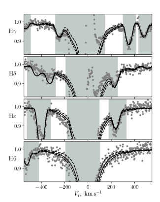
Figure 4: Wings of hydrogen lines. The shaded areas are ignored during the fit. Solid lines are for the best-fit values of $\log g.$ Dashed lines indicate uncertainties in the profiles, corresponding to 0.05 dex.

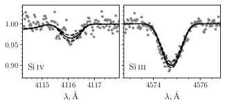
Figure 5: Examples of silicon lines. The solid line is for $T_{\rm eff}=18000$ K, dashed lines correspond to the uncertainty of $\pm 300$ K.

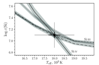
Figure 6: The silicon ionization balance. The solid line is for Si iv $\lambda$4116.1; the dashed, dash-dotted and dotted lines are for Si iii $\lambda$4567.8, 4574.8, 5739.7. The shadowed regions show estimated uncertainties for each line. The star with errorbars marks the intersection point and its uncertainty: the thick line is for uncertainties related with the quality of the fit, the thin line corresponds to the total error, which includes uncertainties in other variables and model limitations, see Sect. 4.5.

4.3 Microturbulence $\xi_{\rm t}$

The microturbulence velocity was derived from the analysis of 34 O ii lines non-blended with lines of other ions. For each line we adjust oxygen abundance $\varepsilon({\rm O})$ for three trial values $\xi_{\rm t}=$7, 10, 13  km s^-1. The obtained dependencies of $\varepsilon({\rm O})$ on $EW$ of the lines are shown in Fig. 7. Slopes of these dependencies were calculated by the error-weighted least-squares. The microturbulence of 7  km s^-1 produces the slope of $k=1.1\pm 0.5,$ while $k=-0.3\pm 0.5$ for $\xi_{\rm t}=10$  km s^-1 and $k=-0.6\pm 0.5$ for $\xi_{\rm t}=13$  km s^-1. Interpolating between these values, we obtain that zero slope should be achieved at $\xi_{\rm t}=9^{+3}_{-1}$  km s^-1. For simplicity we accept $\xi_{\rm t}=10\pm 2$  km s^-1. The weighted mean of $\log\varepsilon({\rm O})=8.59$ with a standard error of 0.02 dex and a standard deviation of 0.11 dex.

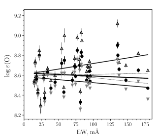
Figure 7: The abundance–equivalent width diagram to determine the microturbulence velocity. Empty triangles, filled circles, and grey triangles show measurements of $\log\varepsilon({\rm O})$ at $\xi_{\rm t}=7,$ 10, 13  km s^-1, correspondingly. The solid lines are linear fits found by the error-weighted least-squares, the thick one corresponds to $\xi_{\rm t}=10$  km s^-1 and the dashed lines around it illustrate the uncertainties in the slope coefficient.

For 62 Ori we obtain $\xi_{\rm t}\sim 30$  km s^-1 and $\log\varepsilon({\rm O})=8.68$ with a scatter of 0.04 dex instead of 0.11 dex for IRAS 18379–1707.

4.4 Chemical abundances

Elemental abundances were determined for the following model parameters: $T_{\rm eff}=18\,000$ K, $\log g=2.25,$ $\xi_{\rm t}=10$ km s^-1. The obtained results are collected in Table 5 and commented below. Uncertainties in the abundances are mostly related to the real irreducible differences between the synthetic and observed spectra rather than the quality of the observations. We suppose that these differences arise due to inaccurate atomic data as well as a noticeable difference between the real, possibly non-hydrostatic, stellar atmosphere and the tlusty models. However, we emphasize that spectrum of the blue supergiant is better reproduced by tlusty models than the spectrum of IRAS 18379–1707. Both objects have similar parameters and show signatures of an outflowing atmosphere, therefore limitations of our modelling should have appeared in both cases. Probably the key difference is a higher mass loss for IRAS 18379–1707, which is significantly more luminous in H$\alpha$.

Table 5: Element abundances determined for IRAS 18379–1707 in $\log\varepsilon=12+\log(n_{\text{X}}/n_{\text{H}})$ and [X/H]=$\log(n_{\text{X}}/n_{\text{H}})-\log(n_{\text{X}\odot}/n_{\text{H}\odot})$

	$\log\varepsilon_{\odot}$	$\log\varepsilon$	[X/H]	$\sigma_{x}$	$\sigma_{\overline{x}}$	N
C	8.43	7.76	–0.67	0.03	0.03	2
N	7.83	7.41	–0.42	0.09	0.04	7
O	8.69	8.59	–0.10	0.11	0.02	34
Ne	7.84	8.39*	0.55	0.17	0.06	8
Mg	7.60	7.30*	–0.30	–	0.15	1
Al	6.45	5.56	–0.89	0.02	0.02	2
Si	7.51	7.10	–0.41	0.05	0.03	4
S	7.12	6.39	–0.73	0.05	0.05	2
Fe	7.50	$\lesssim 7.5$	$<0$	–	–	–

Solar values $\log\varepsilon_{\odot}$ are taken from Asplund et al. (2009). $\sigma_{x}$ and $\sigma_{\overline{x}}$ are the standard deviation and the standard error of mean for $\log\varepsilon.$ N is a number of averaged lines. Abundances marked with * were measured on lines with extended blue wing and probably biased.

He

Almost all helium lines have distortions of the profiles. We selected 10 lines, in which these distortions are minor, and derived the helium abundance by fitting wings of these lines. Regardless of method of abundance determination (from profile fitting or from $EW$) the helium lines show dependence of $\varepsilon$ on $EW$, as if they are formed in gas with $\xi_{\rm t}({\rm He})=30$  km s^-1that is significantly higher than $\xi_{\rm t}({\rm O})=10$  km s^-1, derived from oxygen lines, moreover helium turns to be underabundant $\log\varepsilon({\rm O})=10.65.$ We suppose that these parameters are unrealistic, and were obtained due to various distortions in profiles, in particular, due to unaccounted emission, filled-in photospheric lines, such as directly observed in strong lines (see Fig.  2).

C

In the case of 62 Ori, carbon abundances derived from C ii $\lambda$3921, 4227 and 6578 lines are consistent with each other and result in $\log\varepsilon(\rm C)=7.60.$ The line at 3919 Å is blended with nitrogen, which is enhanced for this star, therefore we exclude this line. Both lines C ii $\lambda$6578/6583 are blue-shifted, and the line at 6583 Å gives $\log\varepsilon({\rm C})=7.70.$ Crowther et al. (2006) using cmfgen models have found $\log\varepsilon({\rm C})=7.65.$ Therefore, tlusty model can reproduce the carbon spectrum of 62 Ori and results are consistent with previous study.

In the case of IRAS 18379–1707, all mentioned lines show large distortion (see Fig. 8), except doublet $\lambda$3919, 3921, which gives $\log\varepsilon({\rm C})=7.76.$ The line at 4227 Å is also consistent with this value, bearing in mind signatures of emission core in its centre.

The line at 6578 Å has a complex shape, which can be interpreted either as a shallow stellar absorption with an additional more narrow absorption feature in the red wing, or as a deep stellar absorption with an emission at the blue wing (see Fig. 8). In the last case we need very high carbon abundance $\log\varepsilon({\rm C})\sim 9,$ which is in contradiction with other lines. The profile of C ii $\lambda$6583 is blended with the forbidden line N ii $\lambda$6584. A joint analysis of the profiles of C ii $\lambda$6578/6583 and [N ii] $\lambda$6548/6584 shows that the observed narrow absorption feature in C ii $\lambda$6578 must also be present in C ii $\lambda$6583, but it is almost completely covered by [N ii] $\lambda$6584. Therefore, both components $\lambda$6578/6583 show profiles with the same distortions.

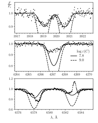
Figure 8: C ii line profiles. Dots are for the observations, lines are for synthetic profiles for various $\log\varepsilon(C).$

N

The nitrogen abundance is measured from 7 individual N ii lines. There are not any significant dependence between $\log\varepsilon(\rm N)$ and $EW$ that means that the N ii lines consistent with the accepted value $\xi_{\rm t}.$ We do not use 4 more lines, which give unreasonable results for 62 Ori. Nitrogen abundance for 62 Ori $\log\varepsilon=8.55$ coincides with previous study by Crowther et al. (2006): $\log\varepsilon=8.55.$

O

The oxygen abundance was determined along with the microturbulence using 34 O ii lines, see Sect. 4.3 and Fig. 7 for details. The obtained value of $\log\varepsilon(\rm O)$ is $8.59\pm 0.02.$ Both stars IRAS 18379–1707 and 62 Ori show similar scatter of $\varepsilon$ measured from various lines $\sigma_{\varepsilon}\approx 0.1$ dex. The mean value of $\varepsilon$ for 62 Ori coincides with the solar 8.69, but higher than value 8.45 deduced by Crowther et al. (2006).

It should be noted that the O i triplet lines at 7771-5 Å are very strong ($EW=2.18$ Å) indicating an extended atmosphere and non-LTE effects. O i $\lambda$6156, 6157 are enhanced in observations and show extended blue wing.

Ne

We selected 8 lines of Ne i. Strong lines show an extended blue wing, such distortions are possible in weak lines, however they are undetectable due to noise. Fitting central and red parts of the profiles gives an abundance of $8.27\pm 0.05,$ the abundance derived from $EW$ measured over the whole profile is $8.40\pm 0.06.$ Neon lines in 62 Ori are significantly weaker and blue-shifted by $\sim 10$  km s^-1, but without enhanced blue wing. Abundance is higher than the solar one by only 0.1 dex and equals to $7.96\pm 0.03.$ Thus, enhancement of neon lines and distortion in their profiles are observed only in IRAS 18379–1707, but absent in the blue supergiant 62 Ori.

Mg, Al

There are two Al iii lines at 5697, 5723 Å, which give $\log\varepsilon=5.58\pm 0.02$ and $5.54\pm 0.02.$ One another line Al iii $\lambda$4480 is weak and blended with strong Mg ii line at 4481 Å, however it probably requires a higher abundance by $0.15-0.2$ dex.

The similar picture is seen in 62 Ori, where Al iii $\lambda$5697, 5723 give $\log\varepsilon=6.29$ and $\log\varepsilon=6.32,$ while Al iii $\lambda$4481 better describes with $\log\varepsilon\approx 6.5,$ which is consistent with solar value 6.45. We note that profiles of Al iii in 62 Ori are slightly distorted: the blue wing is steeper than the red one.

We can conclude that Al abundance in 62 Ori is consistent with the solar value, but in IRAS 18379–1707 it is certainly underabundant at least by 0.7 dex.

The Mg ii $\lambda$4481 shows an extended blue wing, if we fit the red and central part of the profile, we obtain $\log\varepsilon(\rm Mg)=7.0\pm 0.02,$ and $\log\varepsilon(\rm Mg)=7.3,$ if we measure it from EW. The presence of a strong distortion of the profile does not allow us to say that this abundance is correct. In the case of 62 Ori Mg ii $\lambda$4481 show blue-shifted profile by approximately $7$  km s^-1, abundance derived from this line $\log\varepsilon(\rm Mg)=7.3$ (the solar value is 7.6).

Si

The silicon abundance was determined simultaneously with $T_{\rm eff}$ based on three Si iii lines and one Si iv line, see sect. 4.2 and Fig. 6 for details. The obtained value of $\log\varepsilon(\rm Si)$ is $7.1$ with scatter of 0.05 and the standard error of mean 0.03.

S

The observed spectrum contains lines of S ii and S iii, but the S ii $\lambda$5454, 5640, 5647 lines show extended blue wings, at the same time there are the lines (S ii $\lambda$5212, 5322, 5346), which are predicted by tlusty, but absent in observations. We suppose that observed S ii lines are formed in the outflowing gas and cannot be used for the abundance measurements without a proper model of the expanding atmosphere. The sulfur abundance was measured from the S iii $\lambda$4254, 4285 lines, which show symmetric profiles without signs of the outflow.

In the case of 62 Ori we use lines S iii $\lambda$4254, 4285 and S ii $\lambda$5454 and obtain $\log\varepsilon(\rm S)=6.9\pm 0.1$.

Fe

The synthetic spectrum predicts lines of Fe iii at solar abundance of Fe. The absence of these lines in the observed spectrum can impose an upper limit $\log\varepsilon(\rm Fe)<6.8.$ It should be noted that Fe iii $\lambda$5127 and $\lambda$5156 lines appear in the observed spectrum as emission lines.

In the case of 62 Ori Fe iii $\lambda$4005, 4022 give $\log\varepsilon({\rm Fe})=7.0$ and 7.1. More strong lines Fe iii $\lambda$5127, 5156 show peculiarities at the line centre (it has more sharp shape than other lines) and lead to $\log\varepsilon({\rm Fe})=7.8$ and 8.0. If we assume that 62 Ori has near-solar Fe abundance and the lines $\lambda$4005, 4022 underestimate abundance for both stars nearly equally, then we can conclude that IRAS 18379–1707 has $\log\varepsilon(\rm Fe)$ less than the solar value.

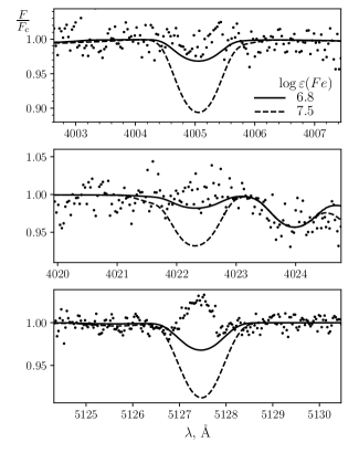
Figure 9: Fe iii line profiles. Dots are for the observations, lines are for synthetic profiles for various $\log\varepsilon(\rm Fe).$

4.5 Error analysis

Uncertainties of the parameters estimated above reflect only the goodness of fit of the observational data. To account uncertainties and limitations in the modelling, we estimate final uncertainties in the parameter $x_{k}$ as

$$\overline{\sigma}_{k}^{2}=\sum\limits_{i}{\left(\frac{\partial x_{k}}{\partial x_{i}}\sigma_{i}\right)^{2}}+\sigma_{C}^{2}+\sigma_{M}^{2}+\sigma_{p}^{2}+\sigma_{\xi m}^{2},$$

where $\frac{\partial x_{k}}{\partial x_{i}}$ reflects change in $x_{k}$ when varying $x_{i}$ at fixed other parameters, these derivatives are collected in Table 6. $\sigma_{i}$ is error in $x_{i}$ related with quality of the fit. In addition to uncertainties of free parameters, we add uncertainties related with continuum placement ($\sigma_{\text{C}}$); metallicity of the model grid ($\sigma_{\text{M}}$): we explore how our results change between models with scaled abundances 0.2 and 0.5 of the solar values; inclusion or not turbulent pressure term in the hydrostatic equation ($\sigma_{p}$); differences in thermal structure of the atmosphere calculated for various values of microturbulence within $\sigma_{\xi}=3$  km s^-1($\sigma_{\xi m}$).

Table 6: The derived parameters, their sensitivity to the model assumptions and final uncertainties.

	$\partial x_{i}/\partial T_{\rm eff}$	$\partial x_{i}/\partial\log g$	$\partial x_{i}/\partial\xi$	$\sigma_{\rm C}$	$\sigma_{\rm M}$	$\sigma_{p}$	$\sigma_{\xi m}$	$x_{i}$	$\sigma_{i}$	$\overline{\sigma}_{k}$
$T_{\text{eff}}$	1	7200	-177	540	400	160	270	18000	300	1000
$\log g$	$10^{-4}$	1	0	0	0.02	0.04	0.03	2.25	0.05	0.08
$\xi$	$-3.3\times 10^{-3}$	0	1	0	2	1	1.8	10	2	3.6
$\log\varepsilon(\text{C})$	$3.5\times 10^{-5}$	-1.9	-0.016	0.06	0.07	0.08	0.01	7.76	0.03	0.16
$\log\varepsilon(\text{N})$	$-2.5\times 10^{-5}$	-0.7	-0.003	0.03	0.03	0.05	0.01	7.41	0.04	0.09
$\log\varepsilon(\text{O})$	$-2.9\times 10^{-4}$	0.7	0	0.05	0.03	0.03	0.02	8.59	0.02	0.13
$\log\varepsilon(\text{Ne})$	$1.1\times 10^{-4}$	-0.7	-0.006	0.04	0.04	0.04	0.01	8.39	0.06	0.11
$\log\varepsilon(\text{Mg})$	$1.1\times 10^{-4}$	-1.4	-0.028	0.02	0.05	0.07	0.01	7.30	0.15	0.20
$\log\varepsilon(\text{Al})$	$-4.5\times 10^{-5}$	0.1	-0.008	0.04	0.04	0.01	0.02	5.56	0.02	0.09
$\log\varepsilon(\text{Si})$	0	0.6	-0.064	0.1	0.01	0	0.02	7.10	0.03	0.18
$\log\varepsilon(\text{S})$	$-1.9\times 10^{-4}$	0.6	-0.020	0.09	0.06	0.01	0.02	6.39	0.05	0.16

4.6 Rotational velocity

The rotational velocity $v\sin i$ was measured from comparison of observed and synthetic spectra on 12 non-blended lines (10 – O ii, 1 – Si iii, 1 – Al iii) without visible distortions. We generated a grid of synthetic spectra for obtained stellar parameters with various rotational velocities. The rotational broadening was calculated directly by integrating intensities produced by synplot.

Line profiles were transformed into velocity space in the stellar rest frame using theoretical line positions and average radial velocity of the star $V_{\rm r}=-124$  km s^-1. After that all profiles were interpolated on a single velocity grid and averaged. Both observed and synthetic profiles were treated in exactly the same manner. A comparison between the averaged profiles was carried out in Fourier space (, 1976). The first zero in the Fourier transform $|\tilde{f}|$ gives $v\sin i$ about 37  km s^-1, and shape of low-frequency part of $|\tilde{f}|$ gives $\sigma_{f}=22$  km s^-1 for the Gaussian contribution (see Fig. 10).

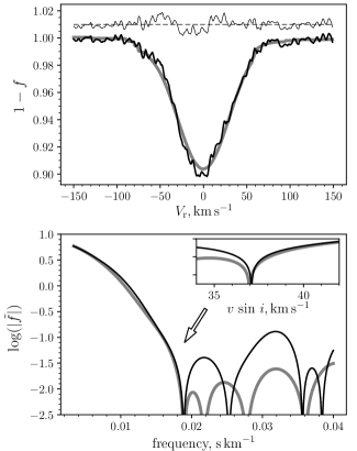
Figure 10: The average profiles (the upper panel) and corresponding Fourier transforms (the lower panel). The black lines are for observations, the grey lines are for the synthetic spectrum for $v\sin\,i=37$  km s^-1 and $\sigma_{f}=22$  km s^-1. The thin line on the upper panel is for the residual between the synthetic and observed spectra.

To estimate uncertainty of $v\sin i,$ we performed the following Monte-Carlo calculations. We generated $\sim 10^{5}$ artificial observations, each of which is a synthetic spectrum for $v\sin i=37$  km s^-1, $\sigma_{f}=22$  km s^-1 with a Gaussian noise with $\sigma=0.01,$ which is correspond to the noise in the real observed spectrum. Applying our procedure, we obtain distributions for $v\sin i$ and $\sigma_{f}.$ The distribution for $v\sin i$ is slightly asymmetric, but within $2\sigma$ can be considered as a Gaussian distribution with $\sigma=6$  km s^-1, the distribution of $\sigma_{f}$ looks like a Gaussian with $\sigma=1$  km s^-1. Removing the instrumental contribution from $\sigma_{f}$ reduces it by 1  km s^-1. Summarizing, $v\sin i=37\pm 6$  km s^-1 and the Gaussian contribution is $\sigma_{f}=21\pm 1$  km s^-1, which can include various terms: microturbulence, macroturbulence, instrumental profile, deviations in line positions.

Some asymmetry can be suspected in the observed profile. It manifests itself in deviations from the synthetic profile at velocities –50, –25 and +10  km s^-1, which makes the blue wing more steep, then the red one. If this deviations are real, then they may be signatures of radial expansion of the star or ongoing convection.

5 ANALYSIS OF THE EMISSION LINE SPECTRUM

Due to the rather low temperature of the central star, the emission spectrum of the object still contains a very limited set of lines, which are usually used to diagnose the gas envelope. In addition, in the absence of a flux calibrated spectrum it is not possible to obtain reliable absolute fluxes for the emission lines. However, using the equivalent widths given in Table LABEL:emlines and stellar continuum flux distributions for the atmospheric parameters defined above, we can obtain reliable ratios of fluxes in the emission lines.

5.1 Nebular parameters

Unfortunately, we cannot estimate plasma parameters from [S ii] ratio, since the ratio $I$($\lambda$6716)/$I$($\lambda$6731)=0.35 indicates that the electron density is higher than the critical one (of order $10^{4}$ cm^-3). Due to the absence of the $\lambda$5755 line in the spectrum, we cannot to estimate the electron temperature from the ratio [N ii] ($I$($\lambda$6548)+$I$($\lambda$6584))/$I$($\lambda$5755).

Using the PyNeb analysis package (Luridiana et al., 2015), we obtained $T_{e}$ versus $N_{e}$ contours for the observed [N i] $I$($\lambda$5198)/$I$($\lambda$5200) and [O i] ($I$($\lambda$6300)+$I$($\lambda$6363))/$I$($\lambda$5577) diagnostic ratios of 1.9 and 8.8, respectively. In the $T_{e}$ range from 5 000 to 20 000 K and $\log N_{e}(\rm cm^{-3})$ from 3 to 8, the curves have no intersection. The nebular line ratios for [N i] indicates that these lines are formed in a partial ionized region of $N_{e}\sim 3~{}000$ cm^-3, whereas [O i] nebular/auroral ratio suggest $N_{e}>10^{6}$ cm^-3. Bautista (1999) investigate the effects of photoexcitation of [N i] and [O i] lines by stellar continuum radiation under nebular conditions and found that the [N i] optical lines at 5198 Å and 5200 Å are affected by fluorescence in many objects. In the presence of radiation fields there is no unique solution in terms of $N_{e}$ and $T_{e}$ for an observed [N i] spectrum.

The comparison of the theoretical from Bautista et al. (1996) and the observed line ratio $I$($\lambda$7412)/$I$($\lambda$7379)=0.31 testifies the pure collisional excitation of [Ni ii] lines in the gaseous shell of IRAS 18379–1707 with $N_{e}>10^{6}$ cm^-3. This result is consistent with conclusion Bautista et al. (1996) about strong intercorrelations between [Ni ii] and [O i] emission in gaseous nebulae, which suggests that they stem from coincident zones.

5.2 Expansion velocities

The expansion velocities of the nebula calculated from the formula: $V_{\text{exp}}=1/2(V_{\text{FWHM}}^{2}-V_{\text{instr}}^{2})^{1/2}$, where $V_{\text{FWHM}}$ is the velocity corresponding to the full width at half maximum (FWHM) and $V_{\text{instr}}$ (6  km s^-1) is the instrumental broadening. The adopted $V_{\text{exp}}$ for each ion are given in Table 7. [N ii](1F) $\lambda$6584 line is blended with the absorption component of the C ii(2) $\lambda$6583 and has not been used to estimate the expansion velocity.

In the case of a spherical symmetric expanding envelope, spectral lines should possess the same radial velocity as the central star. Nevertheless, the emission lines are blue-shifted relative to the stellar spectrum, moreover this shift is greater for greater values of $V_{\rm exp}$, see Fig. 11. Such behaviour can be explained if the observer for some reason (for example, due to an intrinsic absorption in the envelope) receives less light from the back parts of the envelope than from the front ones, which leads to the appearance of line asymmetry and the dependence of the line shift on the expansion velocity $V_{\rm exp}$.

The expansion velocities given in Table 7 shows that the low excitation nebula present around the star is slowly expanding. However at present the nebula is very compact and it is not resolved. As the star evolves to higher $T_{\rm eff}$ value it will photoionize the nebula and there will be hot and fast stellar wind from the star, by then the present compact nebula will expand and grow in size. Once we can measure the angular size of the nebula we can calculate the linear size as the distance to the star is known. Using the linear size of the nebula and expansion velocity we can calculate the age of the nebula (for example please see Parthasarathy et al. (1993, 1995) in the case of SAO 244567).

Table 7: Expansion velocities.

Identification	$\lambda_{\text{lab.}}$	$V_{\text{FWHM}}$	$V_{\text{exp}}$
	Å	km s-1	km s-1
[Fe ii](7F)	4287.39	24.12	11.68
[N i](1F)	5197.90	31.14	15.28
[N i](1F)	5200.26	25.77	12.53
[O i](1F)	6300.30	20.79	9.96
[O i](1F)	6363.78	19.22	9.13
[N ii](1F)	6548.05	28.89	14.13
[S ii](2F)	6730.82	25.74	12.52
[Ni ii](2F)	7377.83	28.93	14.15
[Cr ii](3F)	8000.07	33.35	16.40
[C i](3F)	8727.13	18.55	8.77

Figure 11: Expansion velocity vs. $V_{\text{r}}-V_{\text{sys}}$ for different ions with a linear trend of the data (dashed line).

6 DISCUSSION

Based on high-resolution ($R\sim 48~{}000$) observations we have studied the optical spectrum of the early B-supergiant with IR excess IRAS 18379–1707. At wavelengths from 3700 to 8820 Å, numerous absorption and emission lines have been identified, their equivalent widths and corresponding radial velocities have been measured. Using non-LTE model atmospheres, we have obtained the effective temperature $T_{\text{eff}}=18~{}000\pm 1000$ K, gravity $\log g=2.25\pm 0.08$, microturbulence velocity $\xi_{\rm t}=10\pm 4$  km s^-1and rotational velocity $v\sin i=37\pm 6$  km s^-1. The temperature agrees within error limits with the previously determined value from (2004) and is lower than that of Cerrigone et al. (2009) (see Table 1). The parameters $T_{\rm eff}$ and $\log g$ lead from the Straižys (1982) calibration to the spectral type B2-B3I which consistent with B2.5Ia from (1998).

6.1 Abundance

As stressed by Stasińska et al. (2006) after, e.g., Mathis & Lamers (1992), Fe , cannot be used for post-AGB stars as the metallicity indicator in stellar atmospheres because of possible strong depletion in dust grains in a former stage and subsequent ejection of the grains. On the other hand, S  does not get depleted even if there is a dust-gas separation, because S  does not get condensed into dust grains and S  trace the original metallicity of the star. For IRAS 18379–1707 [S /H ]=–0.73, hence we conclude that the star is metal poor. Al  and Si  show deficiency by –0.92, and –0.43 dex, respectively.

One has to note, that in IRAS 18379–1707 the uncertainty on the carbon abundance prevents an accurate C/O number ratio for this star. However, if we accept that the carbon abundance derived from the $\lambda$3919, 3921 and 4267 lines are closer to the truth than that measured from the $\lambda$6578 line, which is associated with a large equivalent width and seems to have its origin in the outflow, then the carbon abundance is $\log\varepsilon(\rm C)=7.76$ and C/O<1.

Stasińska et al. (2006) offered to identify objects that have experienced third dredge-up as those objects in which (C+N+O)/S is larger than in the Sun. The estimates of the CNO abundances in IRAS 18379–1707 indicate that these elements are overabundant with [(C+N+O)/S]$=+0.5\pm 0.2$ suggesting that the products of helium burning have been brought to the surface as a result of third dredge-up on the AGB.

6.2 Mass and luminosity

Our analysis of the high-resolution optical spectrum of IRAS 18379–1707 with other published results (infrared colours similar to PNe, presence of a circumstellar envelope) confirms that the star is indeed in the post-AGB phase.

To determine the stellar mass, we compared $T_{\text{eff}}$ and $\log g$ to stellar evolutionary calculations for H-rich post-AGB stars that have recently been presented by Miller Bertolami (2016). Unfortunately, the models for metallicity of $Z$=0.003 are not yet calculated, so we used two grids with initial metallicities of $Z$=0.010 and $Z$=0.001.

Fig. 12 shows the evolutionary tracks of Miller Bertolami (2016) for metallicities of $Z$ = 0.01 and $Z$ = 0.001 plotted in the $\log T_{\text{eff}}-\log g$ diagram. From the derived atmospheric parameters we find IRAS 18379–1707 to be located between the two mass tracks for $Z$ = 0.01, implying a current mass $M_{\text{c}}$ of 0.58 to 0.64 M_⊙ and a initial mass of the progenitor $M_{\text{ZAMS}}$ of 2.0 to 3.0 M_⊙. The grid with initial metallicity of $Z$ = 0.001 yield a current mass of $M_{\text{c}}=0.58~{}M_{\odot}$ and a initial mass of 1.25 to 1.75 M_⊙. So we estimate the core mass $M_{\text{c}}\sim 0.58M_{\odot}$ and the mass of the progenitor $M_{\text{ZAMS}}\sim 1.5M_{\odot}$.

As seen from Fig. 12 that IRAS 18379–1707 is placed in a region of the $\log T_{\text{eff}}$ and $\log g$ diagram where other hot post-AGB objects have been observed, viz. V886 Her (, 2003), TYC 6234-178-1, LSS 4634, LS 3099, LS IV-12^∘111, LSE 63 (Mello et al., 2012). Here we compare the position of post-AGB stars in the $\log T_{\text{eff}}$–$\log g$ diagram, for which non-LTE analysis has been performed. As noted by (2003) the LTE analyses yielded effective temperature estimates and the gravities significantly higher than those from the non-LTE analyses.

With the core mass $M_{\text{c}}\sim 0.58M_{\odot}$ and $T_{\text{eff}}=18~{}000$ K, the star falls on the horizontal part of the post-AGB evolutionary track on the HR diagram with $\log(L/L_{\odot})\sim 3.95$.

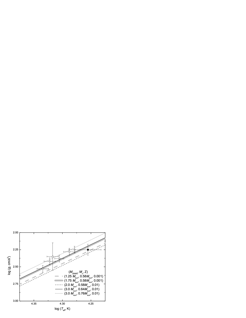
Figure 12: Location of IRAS 18379–1707 (filled circle) in the $\log T_{\text{eff}}-\log g$ plane with $Z$ = 0.001 and $Z$ = 0.01 single-star evolutionary tracks of Miller Bertolami (2016). Also shown are the positions of other hot post-AGB stars: V886 Her (, 2003) (open triangle) and five objects from Mello et al. (2012) (open circles).

6.3 Distance and location in Galaxy

IRAS 18379-1707 is present in the Gaia data release DR2 (, 2018) with the parallax $\pi=0.2593\pm 0.0648$ mas and proper motion $\mu_{\alpha}=-2.065\pm 0.089$ mas/yr, $\mu_{\delta}=0.410\pm 0.075$ mas/yr. Gaia DR2 parallaxes have a zero-point error that is different for different objects (2018), but for weak stars it averages –0.05 mas, in the direction of increasing parallaxes and, accordingly, decreasing distances. If we add 0.05 to parallax 0.2593, then we get 0.3093 mas and the distance to the object decreases to $d=3.24^{+0.86}_{-0.57}$ kpc.

The star is located at the Galactocentic distance $r_{g}\sim 4.5$ kpc with the azimuthal angle $\theta=11.^{\circ}8$ between the Sun–Galactic center line and the direction to the star and at the distance from the Galactic plane of $z=-306_{-81}^{+54}$ pc. Its velocity components calculated in the direction of the Galactic radius vector ($U$), azumuthal direction ($V$), and perpenducular to the Galactic plane ($W$) are 147, 171, 50  km s^-1, respectively. The star rotates slower than it should due to the Galactic rotation curve by 58  km s^-1($V_{res}=-58$  km s^-1). The total velocity with respect to the Galactic center is 230 km/s. Generally the velocity deviations from the circular velocity can be due to perturbation from the Galacic bar (Melnik et al., 2019).

Among post-AGB supergiants there are few high velocity stars. Among the cooler post-AGB supergiants HD 56126 (+105  km s^-1) (Parthasarathy et al., 1992), HD 179821 (+81.8  km s^-1) (Parthasarathy et al., 2019), were found and among hotter post-AGB stars LS III +52^∘24 (IRAS 22023+5249) (–148  km s^-1) (, 2012), and BD+33^∘2642 (–100  km s^-1) (Napiwotzki et al., 1994).

Using the determined luminosity from Sect. 6.2, $V=11.93$ mag (, 1998), $E(B-V)=0.71$ mag from (2004), $R_{V}=3.1$ and the bolometric corrections ($BC$) in the calibration of (1996) we derived the distance $d\sim 3.8$ kpc from $\log d=V+5-3.1E(B-V)-M_{bol\odot}-BC+2.5\log(L/L_{\odot})$. This value is close to that derived from the Gaia parallax measurement. This result also confirms the conclusion that IRAS 18379–1707 is a low-mass post-AGB star, and not a massive Population I B supergiant with a typical luminosity of about $\log(L/L_{\odot})\sim 5.0$.

6.4 Photometric variability

IRAS 18379–1707 is suspected of variability and in the General Catalog of Variable Stars (Samus et al., 2017) is designated as NSV 24542, but the type of variability has not yet been determined.

To analyse the photometric variability, we used two sources of data: All Sky Automated Survey (ASAS-3, (2002)) and All Sky Automated Survey for Super-Novae (ASAS-SN, (2014, 2017)). IRAS 18379–1707 was monitored with the ASAS-3 in $V$ photometric band since February 22, 2001 up to October 6, 2009. We used the good quality (symbol A) measurements made with aperture 1 (15$\arcsec$). ASAS-SN $V$-band data span a time interval from March 21, 2015 to September 23, 2018. The ASAS-3 and ASAS-SN data points are shown in Fig. 13 with their corresponding errorbars. The mean brightness in $V$ band with the standard deviation ($SD$), the number of observations (N) and the mean accuracy of the measurements ($\sigma V$) from ASAS and ASAS-SN are listed in Table 8.

The star displays a brightness variation on a scale of a few nights with a maximum amplitude (peak-to-peak) of up to 0.2 mag in the $V$ band. We performed a period analysis with the period-finding program Period04 (Lenz & Breger, 2005) and we did not find any reliable period to describe the variations. The pattern of variability for IRAS 18379–1707 is very similar to the photometric behaviour of the other hot post-AGB, early B supergiants with IR excesses (, 2007, 2013, 2014, 2018). All of them display fast irregular photometric variability with amplitudes from 0.2 to 0.4 in the $V$-band. For a number of the hot post-AGB objects, spectral variability was also detected, which is expressed in line variations in both shape and intensity (, 1993; García-Lario et al., 1997b; , 2012, 2014). These variations, as well as photometric variability, occur on a scale of a few days. In addition, IRAS 18379–1707, as well as other hot post-AGB objects (, 2005; Mello et al., 2012; , 2003), shows the H$\alpha$ P-Cygni profile ongoing mass-loss. Therefore, most likely, the photometric variability is associated with a variable stellar wind. However, other causes of variability are not excluded, for example, short-period pulsations for the detection of which observations with better temporal resolution than those of ASAS and ASAS-SN are necessary.

Table 8: Summary of photometric observations of IRAS 18379–1707

Source	$V$, mag	$SD$, mag	N	$\sigma V$, mag
ASAS-3	12.01	0.11	460	0.041
ASAS-SN	12.00	0.08	720	0.013

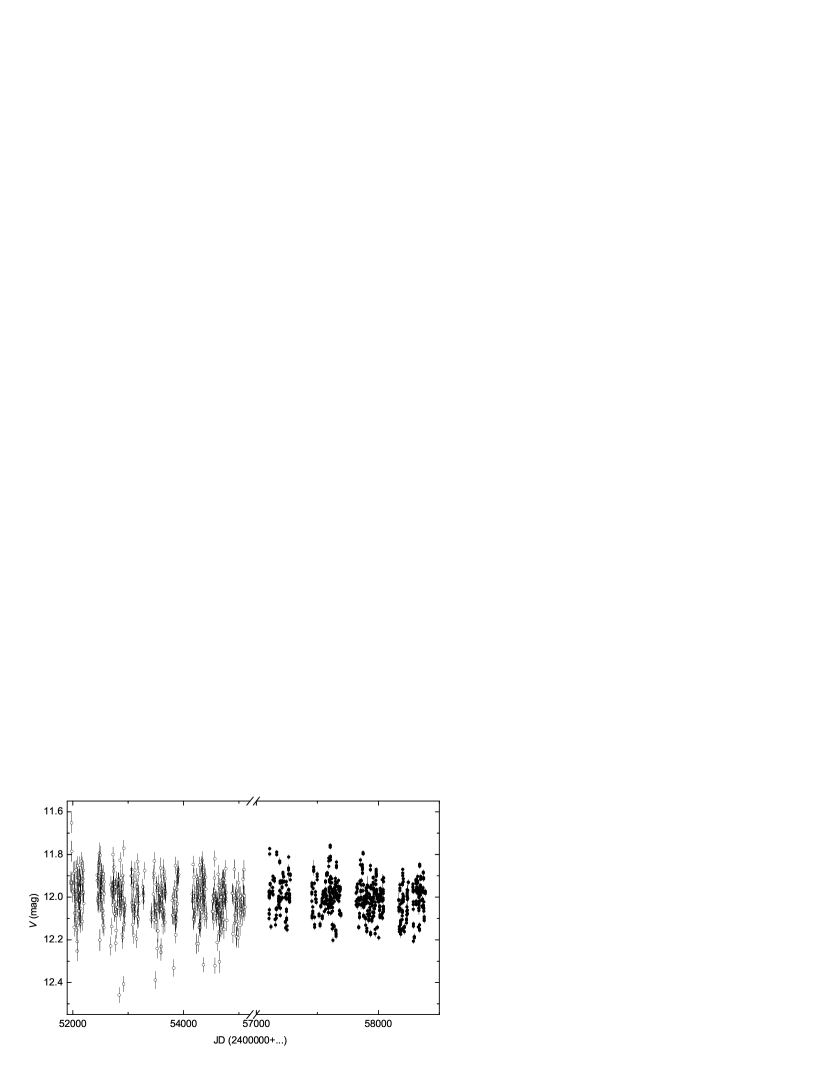
Figure 13: ASAS-3 (the open circles) and ASAS-SN (the filled circles) light curve of IRAS 18379–1707 from 2009 to 2018.

7 CONCLUSIONS

From a non-LTE analysis of high resolution spectrum of hot post-AGB candidate IRAS 18379–1707 (LS 5112) we find its $T_{\text{eff}}=18000$ K, $\log g=2.25$ and find that it is a metal-poor [M/H]=–0.6 high velocity star $V_{r}=-124$  km s^-1. Oxygen, Carbon and Nitrogen are slightly overabundant relative to Sulfur suggesting that the products of helium burning have been brought to the surface as a result of third dredge-up on the AGB.

We found permitted and forbidden emission lines of several elements in its spectrum. The nebular emission lines indicates the presence of a low excitation nebula around this post-AGB star in agreement with other studies mentioned in the paper (see for example (2015) who found evidence for the presence of bipolar flow). The presence of several P-Cygni lines in the spectrum indicates ongoing post-AGB mass-loss. The mean radial velocity as measured from emission features of the envelope is $V_{\text{r}}=-130.9\pm 0.5$  km s^-1.

We measured the radial velocities from the Doppler shifts of many spectral lines and discovered that LS 5112 is a high velocity star.

From the Gaia DR2 parallax we find the distance to be 3.2 kpc. From the derived $T_{\text{eff}}$, $\log g$, and luminosity and placing it on the recent post-AGB evolutionary tracks we conclude that it is a post-AGB star of core mass about 0.58$M_{\odot}$.

8 ACKNOWLEDGMENTS

This research has made use of the SIMBAD database, operated at CDS, Strasbourg, France, and SAO/NASA Astrophysics Data System. AD acknowledges the support from the Program of development of M.V. Lomonosov Moscow State University (Leading Scientific School ‘Physics of stars, relativistic objects and galaxies’). We would like to thank Dr. A.M. Melnik for her help in calculations related to the kinematics of the star. We are also grateful to the anonymous referee for the careful reading of the manuscript and the numerous important remarks that helped to improve the paper.

Appendix A Emission lines in the spectrum of IRAS 18379–1707

Table 9: Emission lines in the spectrum of IRAS 18379–1707.

$\lambda_{\text{obs.}}$	$\lambda_{\text{lab.}}$	Identification	$EW$	$V_{\text{r}}$
Å	Å		Å	km s-1
3854.42	3856.02	Si ii(1)	0.072	-124.47
3860.98	3862.59	Si ii(1)	0.043	-124.81
4199.31	4201.17	[Ni ii]	0.007	-132.93
4242.15	4243.98	[Fe ii](21F)	0.024	-129.01
4274.96	4276.83	[Fe ii]	0.030	-131.25
4285.49	4287.39	[Fe ii](7F)	0.092	-133.40
4350.85	4352.78	[Fe ii](21F)	0.015	-132.97
4357.39	4359.34	[Fe ii](7F)	0.069	-133.83
4366.31	4368.13	O i(5)	0.019	-124.43
4411.83	4413.78	[Fe ii](6F)	0.054	-132.74
4414.31	4416.27	[Fe ii](6F)	0.041	-133.13
4450.08	4452.11	[Fe ii](7F)	0.026	-136.69
4455.96	4457.95	[Fe ii](6F)	0.029	-133.54
4472.94	4474.91	[Fe ii](7F)	0.015	-131.72
4772.57	4774.74	[Fe ii](20F)	0.014	-136.17
4812.41	4814.55	[Fe ii](20F)	0.055	-132.98
4887.44	4889.63	[Fe ii](4F)	0.014	-134.18
4903.19	4905.35	[Fe ii](20F)	0.021	-131.95
5038.90	5041.03	Si ii(5)	0.049	-126.67
5053.90	5055.98	Si ii(5)	0.122	-123.24
5109.38	5111.63	[Fe ii](19F)	0.017	-131.91
5125.29	5127.35	Fe iii(5)	0.017	-120.21
5153.94	5156.12	Fe iii(5)	0.021	-127.45
5156.50	5158.81	[Fe ii](19F)	0.064	-134.15
5195.62	5197.90	[N i](1F)	0.062	-131.49
5197.96	5200.26	[N i](1F)	0.033	-132.23
5259.30	5261.61	[Fe ii](19F)	0.048	-131.50
5271.02	5273.35	[Fe ii](18F)	0.023	-132.46
5296.69	5298.97	O i(26)	0.020	-128.66
5331.29	5333.65	[Fe ii](19F)	0.014	-132.66
5510.27	5512.77	O i(25)	0.018	-135.96
5552.51	5554.95	O i(24)	0.023	-131.71
5574.94	5577.34	[O i](3F)	0.021	-128.92
5887.41	5889.95	Na i(1)	0.068	-129.30
5893.35	5895.92	Na i(1)	0.020	-130.82
5955.16	5957.56	Si ii(4)	0.153	-120.95
5976.39	5978.93	Si ii(4)	0.258	-127.37
6043.71	6046.38	O i(22)	0.057	-132.12
6297.62	6300.30	[O i](1F)	0.220	-127.55
6344.41	6347.11	Si ii(2)	0.138	-127.53
6361.07	6363.78	[O i](1F	0.063	-127.52
6368.65	6371.37	Si ii(2)	0.050	-127.93
6545.12	6548.05	[N ii](1F)	0.075	-134.18
6580.47	6583.45	[N ii](1F)	0.222	-135.85
6663.90	6666.80	[Ni ii](2F)	0.042	-130.63
6713.50	6716.44	[S ii](2F)	0.020	-131.05
6727.83	6730.82	[S ii](2F)	0.057	-133.09
6999.05	7002.13	O i(21)	0.055	-131.71
7152.01	7155.17	[Fe ii]	0.022	-132.58
7228.40	7231.33	C ii(3)	0.146	-121.32
7233.58	7236.42	C ii(3)	0.241	-117.49
7251.15	7254.36	O i(20)	0.078	-132.61
7374.62	7377.83	[Ni ii](2F)	0.312	-130.27
7408.39	7411.61	[Ni ii](2F)	0.099	-130.30
7420.40	7423.64	N i(3)	0.017	-130.72
7464.96	7468.31	N i(3)	0.071	-134.69
7509.92	7513.08	Fe ii(J)	0.046	-126.09
7873.78	7877.05	Mg ii(8)	0.144	-124.45
7893.01	7896.37	Mg ii(8)	0.296	-127.56
7996.50	8000.07	[Cr ii](1F)	0.108	-133.60
8121.77	8125.30	[Cr ii](1F)	0.090	-130.18
8231.18	8234.64	Mg ii(7)	0.156	-125.96
8238.76	8242.34	N i(7)	0.083	-130.21
8297.14	8300.99	[Ni ii](2F)	0.065	-138.90
8304.71	8308.51	[Cr ii](1F)	0.048	-137.07
8442.76	8446.25	O i(3)	2.452	-124.00
8613.11	8616.96	[Fe ii](13F)	0.071	-134.02
8679.50	8683.40	N i(1)	0.072	-134.82
8699.50	8703.25	N i(1)	0.108	-129.12
8707.89	8711.70	N i(1)	0.068	-131.25
8723.44	8727.13	[C i](3F)	0.095	-126.66
9114.36	9218.25	Mg ii(1)	1.310	-126.51

Appendix B Radial velocities of the stellar absorption lines

Table 10: Absorption lines used for measurement of the stellar radial velocity.

ion	$\lambda_{\rm lab}$	$E_{l}$	$EW$	$V_{\rm r}$	$\sigma_{V_{\rm r}}$
	Å	eV	mÅ	km s-1	km s-1
He i	3867.49	21.0	120	-130.3	2.6
He i	3871.78	21.2	96	-121.5	2.7
O ii	3911.97	25.7	77	-123.8	1.5
C iib	3919.14	16.3	105	-129.4	2.0
C iib	3920.61	16.3	100	-125.7	1.5
He i	3926.53	21.2	169	-122.5	1.2
O ii	3945.04	23.4	53	-128.0	2.7
O ii	3973.21	23.4	82	-127.8	1.3
N ii	3995.00	18.5	114	-124.9	1.1
O ii	4069.78	25.6	140	-125.1	1.1
O ii	4072.14	25.6	112	-123.8	1.3
O ii	4075.85	25.7	117	-125.6	0.8
O ii	4153.29	25.8	72	-126.7	1.7
He i	4169.05	21.2	66	-124.8	1.4
O ii	4185.44	28.4	56	-128.5	1.9
O ii	4189.78	28.4	64	-129.3	1.4
S iii	4253.61	18.2	88	-124.0	1.3
O ii	4317.15	23.0	106	-126.3	0.9
O ii	4319.63	23.0	103	-124.9	0.8
O ii	4345.52	23.0	105	-123.6	1.0
O ii	4347.44	25.7	53	-124.7	1.9
O ii	4349.40	23.0	153	-121.1	0.6
O ii	4351.27	25.7	58	-126.4	0.8
O ii	4366.89	23.0	100	-127.3	1.0
O ii	4414.90	23.4	122	-123.6	0.8
He i	4437.54	21.2	75	-126.1	1.2
Si iii	4552.62	19.0	225	-120.9	0.5
Si iii	4567.84	19.0	187	-122.8	0.6
Si iii	4574.75	19.0	121	-125.3	0.7
O ii	4590.97	25.7	93	-128.2	0.8
O ii	4596.16	25.7	89	-126.8	1.0
O ii	4638.85	23.0	95	-124.4	0.8
O ii	4641.81	23.0	130	-123.1	0.7
O ii	4649.14	23.0	183	-118.7	0.6
O ii	4650.80	23.0	106	-124.5	0.9
O ii	4661.63	23.0	101	-125.0	0.6
O ii	4676.24	23.0	100	-124.0	0.8
O ii	4699.16	28.5	62	-126.2	1.1
O ii	4705.34	26.2	70	-125.3	1.0
O ii	4710.01	26.2	38	-129.4	1.8
Si iii	4819.71	26.0	54	-128.6	1.6
Si iii	4828.96	26.0	43	-125.6	2.0
O ii	4924.47	26.3	73	-131.3	1.3
N ii	5001.37	20.6	81	-127.8	1.1
N ii	5005.15	20.7	56	-128.8	1.9
N ii	5666.62	18.5	65	-123.8	1.4
N ii	5676.02	18.5	71	-123.4	1.3
N ii	5679.56	18.5	135	-122.2	1.0
Al iii	5696.57	15.6	95	-123.7	0.9
Al iii	5722.71	15.6	55	-130.5	1.8
Si iii	5739.74	19.7	161	-119.9	0.5

To more accurate treatment of blended/multicomponent lines, we measure $\lambda_{\rm lab}$ using the theoretical spectrum generated by synplot. ^b marks probably blended lines.

Table 11: Absorption lines with extended blue wings.

ion	$\lambda_{\rm lab}$	$E_{l}$	$EW$	$V_{\rm r}$	$\sigma_{V_{\rm r}}$
	Å	eV	mÅ	km s-1	km s-1
Si ii	4128.07	9.8	113	-141.7	1.5
Si ii	4130.90	9.8	123	-145.1	1.5
Mg ii	4481.20	8.9	211	-137.3	1.0
S ii	5640.01	14.1	142	-129.3	0.9
S ii	5647.01	13.7	91	-140.4	1.6
S ii	5659.79	13.7	49	-125.1	2.3
Ne i	5852.49	16.8	77	-144.2	1.1
S ii	6312.75	14.2	75	-147.0	2.8
Ne i	6334.43	16.6	46	-134.8	1.9
Ne i	6402.25	16.6	177	-128.7	0.7
Ne i	7032.41	16.6	71	-137.3	1.6

References

- (1) Arenou F., Luri X., Babusiaux C., Fabricius C., Helmi A. et al., 2018, A&A, 616, A17
- (2) Arkhipova V.P., Esipov V.F., Ikonnikova N.P., Komissarova G.V., Noskova R.I., 2007, Astron. Lett., 33, 604
- (3) Arkhipova V.P., Burlak M.A., Esipov V.F., Ikonnikova N.P., Komissarova G.V., 2012, Astron. Lett., 38, 157
- (4) Arkhipova V.P., Burlak M.A., Esipov V.F., Ikonnikova N.P., Komissarova G.V., 2013, Astron. Lett, 39, 619
- (5) Arkhipova V.P., Burlak M.A., Esipov V.F., Ikonnikova N.P., Kniazev A.Yu., Komissarova G.V., Tekola A., 2014, Astron. Lett., 40, 485
- (6) Arkhipova V.P., Parthasarathy, M., Ikonnikova N.P., Ishigaki M., Hubrig S., Sarkar G., Kniazev A.Y., 2018, MNRAS, 481, 3935
- Asplund et al. (2009) Asplund M., Grevesse N., Sauval A.J., Scott P., 2009, ARAA, 47, 481
- Beitia-Antero & Gómez de Castro (2016) Beitia-Antero L., Gómez de Castro A.I., 2016, A&A, 596A, 49
- Bailer-Jones et al. (2018) Bailer-Jones C.A.L., Rybizki J., Fouesneau M., Mantelet G., Andrae R., 2018, ApJ, 156:58
- Bautista et al. (1996) Bautista M.A., Peng J., Pradhan A.K., 1996, ApJ, 460, 372
- Bautista (1999) Bautista M.A., 1999, ApJ, 527, 474
- Bowen (1947) Bowen I. S., 1947, PASP, 59, 196
- Cerrigone et al. (2009) Cerrigone L., Hora J.L., Umana G., Trigilio C., 2009, ApJ, 703, 585
- Crowther et al. (2006) Crowther P.A., Lennon D.J., Walborn N.R., 2006, A&A, 446, 279
- (15) Gaia Collaboration; Brown A. G. A., Vallenari A., Prusti T. et al., 2018, A&A, 616, 10
- García-Lario et al. (1997a) García-Lario P., Manchado A., Pych W., Pottasch S. R., 1997a, A&AS, 126, 479
- García-Lario et al. (1997b) García-Lario P., Parthasarathy M., de Martino D., Sanz Fernández de Córdoba L., Monier R., Manchado A., Pottasch S. R., 1997b, A&A, 326, 1103
- (18) Gauba G., Parthasarathy M., 2003, A&A, 407, 1007
- (19) Gauba G., Parthasarathy M., 2004, A&A, 417, 201
- (20) Gledhill T. M., Forde K. P., 2015, MNRAS, 447, 1080
- Haucke et al. (2018) Haucke M., Cidale L.S., Venero R.O.J., Curé M., Kraus M., Kanaan S., Arcos C., 2004, A&A, 614, 91
- Hrivnak et al. (2004) Hrivnak B.J., Kelly D.M., Su K.Y.L., 2004, in ASP Conf. Ser. 313, Asymmetric Planetary Nebulae III, ed. M. Meixner et al. (San Francisco: ASP), 175
- (23) Hobbs L.M., York D.G., Snow T.P., Oka T., Thorburn J.A., Bishof M., Friedman S.D., McCall B.J., Rachford B., Sonnentrucker P., Welty D.E., 2008, ApJ, 680, 1256
- Hubeny & Lanz (1995) Hubeny I., Lanz T., 1995, ApJ, 439, 875
- (25) Kaufer A., Stahl O., Tubessing S. et al., 1999, The Messenger, 95, 8
- (26) Kausch W., Noll S., Smette A., Kimeswenger S., Barden M., Szyszka C., Jones A.M., Sana H., Horst H., Kerber F., 2015, A&A, 576, A78.
- (27) Kelly D.M., Hrivnak B.J., 2005, ApJ, 629, 1040
- (28) Klochkova V.G., Chentsov E.L., Panchuk V.E., Sendzikas E.G., Yushkin M.V., 2014, Astrophys. Bull., 69, 439
- (29) Kochanek C.S., Shappee B.J., Stanek K.Z., Holoien T.W.-S., Thompson, Todd A. et al., 2017, PASP, 129:104502
- (30) Lemke M., 1997, A&AS, 122, 285
- Lenz & Breger (2005) Lenz P., Breger M., 2005, CoAst, 146, 53
- Luna et al. (2008) Luna R., Cox N.L.J., Satorre M.A., García Hernández D.A., Suárez O., García Lario P., 2008, A&A, 480, 133
- Luridiana et al. (2015) Luridiana V., Morisset C., Shaw R.A., 2015, A&A, 573, 42
- Mathis & Lamers (1992) Mathis J.S., Lamers H.J.G.L.M., 1992, A&A, 259, 39
- Mello et al. (2012) Mello D.R.C., Daflon S., Pereira C.B., Hubeny I., 2012, A&A, 543, A11
- Melnik et al. (2019) Melnik A.M., 2019, MNRAS, 485, 2106
- Miller Bertolami (2016) Miller Bertolami M.M., 2016, A&A, 588, A25
- Moore (1945) Moore C. E., 1945, A Multiplet Table of Astrophysical Interest. Princeton Univ. Observatory, Princeton
- Napiwotzki et al. (1994) Napiwotzki R., Heber U., Köppen J., 1994, A&A, 292, 239
- Nyman et al. (1992) Nyman L.-A., Booth R.S., Carlstrom U., Habing H.J. et al., 1992, A&AS, 93, 121
- (41) Parthasarathy M., 1993, ApJ, 414, L109
- Parthasarathy et al. (1992) Parthasarathy M., García-Lario P., Pottasch S.R., 1992, A&A, 264, 159
- Parthasarathy et al. (1993) Parthasarathy M., García-Lario P., Pottasch S.R., Manchado A., Clavel J., de Martino D., van de Steene G.C.M., Sahu K.C., 1993, A&A, 267, L19
- Parthasarathy et al. (1995) Parthasarathy M., García-Lario P., de Martino D., Pottasch S.R., Kilkenny D., Martinez P., Sahu K.C., Reddy B.E., Sewell B.T., 1995, A&A, 300, L25
- Parthasarathy et al. (2019) Parthasarathy M., Jasniewicz G., Thěvenin F., 2019, Ap&SS, 364, 25
- (46) Parthasarathy M., Vijapurkar J., Drilling J.S., 2000, A&AS, 145, 269
- Preite-Martinez (1988) Preite-Martinez A., 1988, A&AS, 76, 317
- (48) Pojmanski G., 2002, Acta Astron., 52, 397
- (49) Reed B.C., 1998, ApJS, 115, 271
- (50) Ryans R.S.I., Dufton P.L., Mooney C.J., Rolleston W.R.J., Keenan F.P., Hubeny I., Lanz T., 2003, A&A, 401, 1119
- Samus et al. (2017) Samus N.N., Kazarovets E.V., Durlevich O.V., Kireeva N.N., Pastukhova E.N., 2017, Astron. Rep., 61, 80
- (52) Sarkar G., Parthasarathy M., Reddy B.E., 2005, A&A, 431, 1007
- (53) Sarkar G., García-Hernández D.A., Parthasarathy M., Manchado A., García-Lario P., Takeda Y., 2012, MNRAS, 421, 679
- (54) Shappee B.J., Prieto J.L., Grupe D., Kochanek C.S., Stanek K. Z., De Rosa G., 2014, ApJ, 788:48
- (55) Szczerba R., Siódmiak N., Stasińska G., Borkowski J., 2007, A&A, 469, 799
- (56) Smith M.A., Gray D.F., 1976, PASP, 88, 809
- Smoker et al. (2004) Smoker J.V., Lynn B.B., Rolleston W.R.J., Kay H.R.M., Bajaja E., Poppel W.G.L., Keenan F.P., Kalberla P.M.W., Mooney C.J., Dufton P.L., Ryans R.S.I., 2004, MNRAS, 352, 1279
- Stasińska et al. (2006) Stasińska G., Szczerba R., Schmidt M., Siódmiak N., 2006, A&A, 450, 701
- Straižys (1982) Straižys V., 1982, Metal-Deficient Stars. Mokslas, Vilnius
- (60) Stephenson C.B., Sanduleak N., 1971, Publ. Warner and Swasey Obs., 1, part no 1, 1
- (61) Umana G., Cerrigone L., Trigilio C., Zappalà R.A., 2004, A&A, 428, 121
- (62) Vacca W.D., Garmany C.D., Shull J.M., 1996, ApJ, 460, 914
- (63) Venn K.A., Smartt S.J., Lennon D.J., Dufton P.L., 1998, A&A, 334, 987