Electromagnetism, Axions, and Topology:
a first-order operator approach to constitutive responses provides greater freedom

Abstract

We show how the standard constitutive assumptions for the macroscopic Maxwell equations can be relaxed. This is done by arguing that the Maxwellian excitation fields ($\boldsymbol{D}$, $\boldsymbol{H}$) should be dispensed with, on the grounds that they (a) cannot be measured, and (b) act solely as gauge potentials for the charge and current. In the resulting theory, it is only the links between the fields ($\boldsymbol{E}$, $\boldsymbol{B}$) and the charge and current ($\rho$, $\boldsymbol{J}$) that matter; and so we introduce appropriate linear operator equations that combine the Gauss and Maxwell-Ampère equations with the constitutive relations, eliminating ($\boldsymbol{D}$, $\boldsymbol{H}$). The result is that we can admit more types of electromagnetic media – notably, the new relations can allow coupling in the bulk to a homogeneous axionic material; in contrast to standard electromagnetism (EM) where any homogeneous axion-like field is completely decoupled in the bulk, and only accessible at boundaries. We also consider a wider context, including the role of topology, extended non-axionic constitutive parameters, and treatment of Ohmic currents. A range of examples including an axionic response material is presented, including static electromagnetic scenarios, a possible metamaterial implementation, and how the transformation optics paradigm would be modified. Notably, these examples include one where topological considerations make it impossible to model using ($\boldsymbol{D}$, $\boldsymbol{H}$).

There is a popular summary in appendix D.

I Introduction

Maxwell’s equations rely Jackson (1999); Reitz et al. (1980) on the electromagnetic constitutive relations (EMCR), which provide the crucial information relating the excitation fields ($\boldsymbol{D}$, $\boldsymbol{H}$) to the electromagnetic fields ($\boldsymbol{E}$, $\boldsymbol{B}$). In the simplest cases, these constitutive relations are expressed as a simple – homogeneous and isotropic – permittivity and permeability, but the full EMCR allow a much greater freedom. Arguably, the EMCR are the unsung heroes of electromagnetics: without them Maxwell’s equations would be underdetermined and lose predictive power. Because of this central role for the EMCR, a re-examination of the fundamental assumptions behind them has a significant potential to open up new opportunities for electromagnetic metamaterials.

Here, we wish to avoid using ($\boldsymbol{D}$, $\boldsymbol{H}$) because not only is their measurability controversial Gratus et al. (2019a), but they may also have a multi-valued nature Gratus et al. (2019b). In this article, we present a minimal extension to standard Maxwell theory which combines the usual constitutive relations and both the Gauss’s and the Maxwell-Ampère laws. The resulting theory uses new “first order” operators (${{\Psi}}^{E}_{\rho}$, ${{\Psi}}^{B}_{\rho}$, ${{\Psi}}^{E}_{J}$, ${{\Psi}}^{B}_{J}$) that only act on the measurable Gratus et al. (2019a, b) Maxwell fields ($\boldsymbol{E}$, $\boldsymbol{B}$), connecting them to the sources ($\rho$, $\boldsymbol{J}$). As a result the Maxwellian excitation fields ($\boldsymbol{D}$, $\boldsymbol{H}$) are eliminated.

A significant feature of our approach is that our program admits constitutive relations that allow coupling to axion-like terms in a less restrictive way than is usual; notably in the case of homogeneous systems or those with a non-trivial topology. In the latter case, we give an example where it is not possible to model the material using standard constitutive relations. We also suggest an experimental scenario where such an axionic field can be emulated. Although a discussion of axions in the context of EM is an established area of research Tobar et al. (2019); Visinelli (2013), this usually occurs in the context of an added coupling between the Maxwell fields and the field of an axion particle. This contrasts with our axionic response terms, which result from a constitutive property of the background medium. Notably, the Lagrangian for coupling EM to a particle physics type axion field (${\Xi}$) has the form Tobar et al. (2019); Visinelli (2013)

$$L =\tfrac{1}{2}\left(\boldsymbol{E}\cdot\boldsymbol{E}-\boldsymbol{B}\cdot\boldsymbol{B}\right)+\boldsymbol{A}\cdot\boldsymbol{J}$$

$$\qquad+g_{{\Xi}}\,{\Xi}\,\boldsymbol{E}\cdot\boldsymbol{B}\pm\tfrac{1}{2}g_{{\Xi}}^{2}\left[\left(\partial_{t}{}{\Xi}\right)^{2}-\left({\nabla{\Xi}}\right)^{2}\right].$$ (1)

where $g_{{\Xi}}$ is the massless axion coupling. This leads to a coupled Maxwell and axion dynamics, where a background axion field can now influence the EM behaviour.

In the traditional description of a material, the axionic influences appear via a (pseudo-)scalar quantity Hehl and Obukhov (2003) representing a non-zero trace part of the 4-dimensional constitutive tensor. In 3-vector notation, axionic contributions to the excitation fields appear as

$$\boldsymbol{D}_{{\textup{ax\,}}}={\kappa}_{\textup{ax}}\boldsymbol{B}\qquad\textup{and}\qquad\boldsymbol{H}_{{\textup{ax\,}}}=-{\kappa}_{\textup{ax}}\boldsymbol{E}.$$ (2)

where ${\kappa}_{\textup{ax}}$ is a constant representing the axionic response. A simple application of (2) into Maxwell’s equations gives the contribution $\rho_{{\textup{ax\,}}}$ and $\boldsymbol{J}_{{\textup{ax\,}}}$ to the charge and current, due to the axionic field, as

$$\left(\nabla{\kappa}_{\textup{ax}}\right)\cdot\boldsymbol{B}=\rho_{{\textup{ax\,}}}\quad\textup{and}\quad\left(\nabla{\kappa}_{\textup{ax}}\right)\times\boldsymbol{E}+\left(\partial_{t}{\kappa}_{\textup{ax}}\right)\boldsymbol{B}=-\boldsymbol{J}_{{\textup{ax\,}}}$$ (3)

Thus for blocks of homogeneous static materials, the effects of ${\kappa}_{\textup{ax}}$ only appears as a surface term at the boundary of the material.

This response can be considered a special case of a duality rotation Visinelli (2013) of ($\boldsymbol{E}$, $\boldsymbol{B}$), in which the rotation is just $\pi/2$. On the basis of theoretical arguments, Post Post (1997) suggested that the completely antisymmetric part of the constitutive tensor vanishes (i.e. ${\kappa}_{\textup{ax}}=0$) for all naturally occurring media. Subsequently, Lakhtakia and Weiglhofer proposed that this so-called Post constraint was fundamental and applied to all electromagnetic responses Lakhtakia and Weiglhofer (1996); Lakhtakia and Mackay (2015, 2016). Indeed, provided ${\kappa}_{\textup{ax}}$ does not depend on either position or time then Maxwell’s equations are unaffected by the presence of ${\kappa}_{\textup{ax}}$. However, a piecewise constant axionic response is detectable at boundaries Obukhov and Hehl (2005) where the response can be equivalently cast as either a perfect electrical, or perfect magnetic conductor Lindell and Sihvola (2013). Axionic responses were apparently observed experimentally Hehl et al. (2008) via the magneto-electric effect in Cr₂O₃. More recently axionic responses have also been proposed Li et al. (2010) and observed Wu et al. (2016) in topological insulators. Observations are, however, still controversial, with claims that evidence of Post violation can be explained in other ways Lakhtakia and Mackay (2015). In the domain of particle physics, axions have been proposed as candidates for dark matter Feng (2010).

In this paper, since we generalise the definition of EMCR, we can treat axion-like effects in the manner of bound charge and current sources, which allows them to be seen in the bulk. We will call these constitutive properties an “axionic response”. Moreover, our approach allows the number of potential material parameters that represent an axionic response to increase from one to four.

Our paper is organised as follows: In section II we briefly summarise how constitutive properties usually appear in the context of Maxwell’s equations, and in section III we introduce our new approach; in section IV we then discuss two important topological consequences. Next, in section V we give some examples in media incorporating the new axionic response constitutive effects. We then briefly propose a possible metamechanical axionic response element, introduce how the transformation optics paradigm needs to be modified, and discuss an extension handling Ohmic current and resistance, before concluding in section VII. There are also a number of appendices covering further mathematical details, including a presentation of a spacetime formalism (A), proofs (B), and coordinate-free notation (C).

II Maxwell’s Equations and the constitutive tensor

The macroscopic Maxwell’s equations are perhaps most elegantly expressed in a fully four dimensional spacetime form using exterior calculus Hehl and Obukhov (2003), although spacetime formulations using tensors are also popular (see e.g. Heras and Baez (2008)). Nevertheless, it is the very familiar Gibbs-Heaviside vector calculus form which is most widely used in practical calculations, where they are written as

$$\nabla\cdot\boldsymbol{B} =0,$$ (4)

$$\nabla\times\boldsymbol{E}+\partial_{t}{\boldsymbol{B}} ={\boldsymbol{0}},$$ (5)

$$\nabla\cdot\boldsymbol{D} ={\rho},\qquad\qquad$$ (6)

$$\text{and}\qquad\nabla\times\boldsymbol{H}-\partial_{t}{\boldsymbol{D}} ={\boldsymbol{J}}.$$ (7)

These are augmented with electromagnetic constitutive relations (EMCR) which relate the excitation fields ($\boldsymbol{D}$, $\boldsymbol{H}$) to the electromagnetic fields ($\boldsymbol{E}$, $\boldsymbol{B}$). With the possible exception of the vacuum, EMCR are always an approximation as the underlying structure is either unknown or too complicated to analyse fully.

Usually, the choice of models for the EMCR is limited only by the imagination of the researcher, and the skill of the experimentalist to fabricate and measure. Traditionally these might include fixed values for permittivity and permeability, dynamical models which generate a frequency dependence Jackson (1999); Reitz et al. (1980), an accommodation of anisotropy and birefringence Nye (1985), magnetoelectricity Fiebig (2005); Eerenstein et al. (2006), chirality Hillion (1993); Wang et al. (2009); McCall (2009), nonlinearity New (2011); Boyd (2008), a dependence on temperature or stress Nye (1985), or even spatial dispersion Agranovich and Ginzburg (1984); Belov et al. (2002); Ciraci et al. (2013); Kinsler (2019) – all these can provide good matches to materials found in nature. More complicated empirical models can also be used, with parameters being estimated from or fitted to experimental data. Such descriptions are often remarkably accurate and useful within their own domain, providing us with vital information about the underlying electromagnetic medium, such as the resonances of the individual atoms.

Although a common simple case is where the permittivity and permeability are constant, for anisotropic media these are replaced by tensors ${{\varepsilon}\,}$ and ${{\mu}\,}$, and can even be generalised to include magnetoelectric terms. This general tensor form can be written

$$\boldsymbol{D} =\bar{\bar{\kappa}}^{\textup{DE}}(\boldsymbol{E})+\bar{\bar{\kappa}}^{\textup{DB}}(\boldsymbol{B}),$$ (8)

$$\boldsymbol{H} =\bar{\bar{\kappa}}^{\textup{HE}}(\boldsymbol{E})+\bar{\bar{\kappa}}^{\textup{HB}}(\boldsymbol{B}).$$ (9)

Here $\bar{\bar{\kappa}}^{\textup{DE}}=\varepsilon$ is the permittivity tensor, $\bar{\bar{\kappa}}^{\textup{HB}}=\mu^{-1}$ is the (inverse) permeability tensor and $\bar{\bar{\kappa}}^{\textup{DB}}$ and $\bar{\bar{\kappa}}^{\textup{HE}}$ are magnetoelectric tensors. The number of parameters appearing in these four tensors is 36. In general the tensors ($\bar{\bar{\kappa}}^{\textup{DE}}$, $\bar{\bar{\kappa}}^{\textup{DB}}$, $\bar{\bar{\kappa}}^{\textup{HE}}$, $\bar{\bar{\kappa}}^{\textup{HB}}$) may depend on position, but in a homogeneous medium they are constant. They may also have temporal and spatial dispersion, i.e. if they depend on ($\omega$, $\boldsymbol{k}$). But for a non-dispersive medium, as we consider here, the tensors ($\bar{\bar{\kappa}}^{\textup{DE}}$, $\bar{\bar{\kappa}}^{\textup{DB}}$, $\bar{\bar{\kappa}}^{\textup{HE}}$, $\bar{\bar{\kappa}}^{\textup{HB}}$) have no additional dependence.

Note that any non-dispersive medium is automatically causal in the Kramers-Kronig sense Bohren (2010); Kinsler (2011). Notably, Jackson Jackson (1999) shows that ‘generally correct’ constitutive relations can be based on convolution integrals with respect to their historical or spatial environment. However, whether in the standard EMCR, or in our CMCR defined in the next section, any non-vacuum response in a medium is a result of both (a) its internal dynamics, and (b) its coupling to the EM fields, these must satisfy causality; and thus necessarily be dispersive. However, in appropriately chosen situations, the dispersion may be small enough so that it can reasonably be approximated as negligible.

The nature of the excitation fields ($\boldsymbol{D}$, $\boldsymbol{H}$) is very different to the electromagnetic fields ($\boldsymbol{E}$, $\boldsymbol{B}$), and indeed there is a debate in the literature as to whether or not they are actually physical quantities Heras (2011); Gratus et al. (2019b, a). Notably, it is easy to see that Maxwell’s equations are invariant by adding a gauge ($\phi_{{\textup{g}}}$, $\boldsymbol{A}_{{\textup{g}}}$) to the excitation fields, with the replacements

$$\boldsymbol{D}\to\boldsymbol{D}+\nabla\times\boldsymbol{A}_{{\textup{g}}}\quad\textup{and}\quad\boldsymbol{H}\to\boldsymbol{H}-\nabla\phi_{{\textup{g}}}+\partial_{t}{\boldsymbol{A}_{{\textup{g}}}}.$$ (10)

This gauge freedom is distinct from the usual gauge freedom which is associated only with the potential ($\phi$, $\boldsymbol{A}$) for the ($\boldsymbol{E}$, $\boldsymbol{B}$) fields. These gauge freedoms mean that since Maxwell’s equations only couple with derivatives of ($\boldsymbol{D}$, $\boldsymbol{H}$) or ($\boldsymbol{E}$, $\boldsymbol{B}$) one cannot a priori claim that either are measurable. However, the electromagnetic fields ($\boldsymbol{E}$, $\boldsymbol{B}$) can be directly measured, either directly using the Lorentz force equation or non-locally using the Aharonov-Bohm effect Ehrenberg and Siday (1949); Aharonov and Bohm (1959); Matteucci et al. (2003). This second case is particularly useful as it enables one to measure the electromagnetic fields inside a medium where the Lorentz force may not be useful due to collisions with atoms. In Aharonov-Bohm tests, the electrons only need travel in vacuum outside the medium. In contrast the excitation fields ($\boldsymbol{D}$, $\boldsymbol{H}$) remain not directly measurable, as there is no accepted native Lorentz force-like equation dependent on ($\boldsymbol{D}$, $\boldsymbol{H}$), nor is there any analogous Aharonov-Bohm-like effect for them. Consequently, whenever making claims about the measurability of ($\boldsymbol{D}$, $\boldsymbol{H}$), one has to make assumptions about their nature, for example that they are linearly and locally related ($\boldsymbol{E}$, $\boldsymbol{B}$).

One consequence of the gauge freedom for ($\boldsymbol{D}$, $\boldsymbol{H}$) is that for a homogeneous medium, one of the parameters ${\kappa}_{\textup{ax}}$ in the constitutive tensors $\bar{\bar{\kappa}}^{\textup{DB}}$ and $\bar{\bar{\kappa}}^{\textup{HE}}$ can be ignored. This is the purely axionic field given by (2), and can be removed by setting

$$\phi_{{\textup{g}}} ={\kappa}_{\textup{ax}}\phi,\quad\boldsymbol{A}_{{\textup{g}}}=-{\kappa}_{\textup{ax}}\boldsymbol{A}.$$ (11)

Thus in this case there are only 35 free parameters in the constitutive tensor.

III Proposed Operator Constitutive Relations

Our minimal extension to standard Maxwell theory is motivated by a single crucial step: we decide that the charge and current ($\rho$, $\boldsymbol{J}$) are the most important components of Gauss’ Law (6) and the Maxwell-Ampère equation (7). This enables a simple generalisation of the constitutive properties which enables us to completely remove the non-measurable excitation fields ($\boldsymbol{D}$, $\boldsymbol{H}$) from the description. Therefore we start by rewriting (6) and (7) as

$${\rho} =\nabla\cdot\boldsymbol{D},$$ (12)

$${\boldsymbol{J}} =\nabla\times\boldsymbol{H}-\partial_{t}{\boldsymbol{D}}.$$ (13)

Now we replace the right hand side (RHS) of these with some new operators (${{\Psi}}^{E}_{\rho}$, ${{\Psi}}^{B}_{\rho}$, ${{\Psi}}^{E}_{J}$, ${{\Psi}}^{B}_{J}$) acting directly on ($\boldsymbol{E}$, $\boldsymbol{B}$) rather than – as is usual – a differential operator acting on ($\boldsymbol{D}$, $\boldsymbol{H}$). This replacement is consistent with our discussion above where ($\boldsymbol{D}$, $\boldsymbol{H}$) were seen as a gauge field for the charge and current. A logical consequence of this is to dispense with ($\boldsymbol{D}$, $\boldsymbol{H}$), and directly connect the electromagnetic field to the current. We now implement this idea.

The resulting constitutive relations for media generalised in this way combine Gauss’s Law (6), the Maxwell-Ampère equation (7), and the constitutive tensors (9). They are

$${\rho} ={{\Psi}}^{E}_{\rho}\!\left\langle\boldsymbol{E}\right\rangle+{{\Psi}}^{B}_{\rho}\!\left\langle\boldsymbol{B}\right\rangle,$$ (14)

$$\quad\textup{and}\quad{\boldsymbol{J}} ={{\Psi}}^{E}_{J}\!\left\langle\boldsymbol{E}\right\rangle+{{\Psi}}^{B}_{J}\!\left\langle\boldsymbol{B}\right\rangle,$$ (15)

which we call the combined Maxwell and constitutive relation (CMCR) equations, and where the angle brackets are used to emphasise that the CMCR operators are not tensors, but may also involve the first derivatives of their arguments. These four operators (${{\Psi}}^{E}_{\rho}$, ${{\Psi}}^{B}_{\rho}$, ${{\Psi}}^{E}_{J}$, ${{\Psi}}^{B}_{J}$) take vector fields and output either a scalar or a vector field; their properties are given below in section III.1.

Here $\rho$ and $\boldsymbol{J}$ are the free charges and currents, and (14), (15) are our new microscopic replacements for (12), (13). As is usual, it may in some particular circumstance be useful to move some of the bound charge or (current) effects from the RHS of (14), (15) over to the LHS, re-imagining them as free charges (currents). Indeed, we have complete freedom to split the total charges and currents into free and bound contributions according to our preferred material models; the splitting is not unique (see e.g. Gratus et al. (2019a, b)).

Clearly in (14), ${{\Psi}}^{E}_{\rho}\!\left\langle\boldsymbol{E}\right\rangle$ is the generalisation of the divergence $\nabla\cdot\left(\bar{\bar{\kappa}}^{\textup{DE}}(\boldsymbol{E})\right)$, and ${{\Psi}}^{B}_{\rho}\!\left\langle\boldsymbol{B}\right\rangle$ is a magnetoelectric term. In (15), ${{\Psi}}^{E}_{J}\!\left\langle\boldsymbol{E}\right\rangle$ is the generalisation of $\partial_{t}{}(\bar{\bar{\kappa}}^{\textup{DE}}(\boldsymbol{E}))$ but now can also contain magnetoelectric terms. A careful analysis of the symmetries of the CMCR operators (see appendix B) show that in the homogeneous non-dispersive case they possess 55 free parameters, 20 more than the constitutive tensor $\kappa$ can ever allow. Note that (14) and (15) reduce to Gauss’s Law and the Maxwell-Ampère equation in a vacuum if we set ${{\Psi}}^{E}_{\rho}\!\left\langle\boldsymbol{E}\right\rangle=\varepsilon_{0}\boldsymbol{E}$, ${{\Psi}}^{B}_{J}\!\left\langle\boldsymbol{B}\right\rangle=\nabla\times\mu_{0}^{-1}\boldsymbol{B}$, ${{\Psi}}^{E}_{J}\!\left\langle\boldsymbol{E}\right\rangle=\partial_{t}\varepsilon_{0}\boldsymbol{E}$, and ${{\Psi}}^{B}_{\rho}\!\left\langle\boldsymbol{B}\right\rangle=0$.

We do not consider nonlinear responses in this paper. Nevertheless, one can certainly imagine nonlinear generalizations, although the number of potential CMCR-like constitutive terms would be very large, even for low-order nonlinearities. Our CMCR generalization is a strict superset of the EMCR, and all possible EMCR responses are expressible under our CMCR scheme.

III.1 The CMCR operators

These new CMCR operators (${{\Psi}}^{E}_{\rho}$, ${{\Psi}}^{B}_{\rho}$, ${{\Psi}}^{E}_{J}$, ${{\Psi}}^{B}_{J}$) are not tensors, unlike the standard constitutive tensors ($\bar{\bar{\kappa}}^{\textup{DE}}$, $\bar{\bar{\kappa}}^{\textup{DB}}$, $\bar{\bar{\kappa}}^{\textup{HE}}$, $\bar{\bar{\kappa}}^{\textup{HB}}$) in the traditional constitutive relations (8) and (9). We now specify the properties they must have in order for the fields upon which they act to be consistent with Maxwell’s equations (4) and (5), and with charge conservation.

As a starting point, let us first focus on just the ${{\Psi}}^{E}_{\rho}\!\left\langle\boldsymbol{E}\right\rangle$ term in Eq. (14). Its simplest expression is as the sum of a linear term and a first derivative, i.e. in a coordinate basis it is

$${{\Psi}}^{E}_{\rho}\!\left\langle\boldsymbol{E}\right\rangle =({{\Psi}}^{E}_{\rho})^{i}\ \boldsymbol{E}_{i}+({{\Psi}}^{E}_{\rho})^{0j}\ \partial_{t}{\boldsymbol{E}}_{j}+({{\Psi}}^{E}_{\rho})^{ij}\ \partial_{i}\boldsymbol{E}_{j},$$ (16)

where $i,j\in\left\{1,2,3\right\}$ and we have used implicit summation over repeated indices. However, as we show in appendix B, (16) implies the following three coordinate-free linearity relations:

$${{\Psi}}^{E}_{\rho}\!\left\langle{f}^{2}\boldsymbol{E}\right\rangle =2{f}\,{{\Psi}}^{E}_{\rho}\!\left\langle{f}\boldsymbol{E}\right\rangle-{f}^{2}{{\Psi}}^{E}_{\rho}\!\left\langle\boldsymbol{E}\right\rangle\,,$$ (17)

$${{\Psi}}^{E}_{\rho}\!\left\langle\boldsymbol{E}_{1}+\boldsymbol{E}_{2}\right\rangle ={{\Psi}}^{E}_{\rho}\!\left\langle\boldsymbol{E}_{1}\right\rangle+{{\Psi}}^{E}_{\rho}\!\left\langle\boldsymbol{E}_{2}\right\rangle,$$ (18)

$${{\Psi}}^{E}_{\rho}\!\left\langle\lambda\,\boldsymbol{E}\right\rangle =\lambda\,{{\Psi}}^{E}_{\rho}\!\left\langle\boldsymbol{E}\right\rangle\,,$$ (19)

where $f$ is a scalar field, and $\lambda$ is a real constant. The converse is also true; Eqs. (17)–(19) together imply Eq. (16). We refer to operators (${{\Psi}}^{E}_{\rho}$, ${{\Psi}}^{B}_{\rho}$, ${{\Psi}}^{E}_{J}$, ${{\Psi}}^{B}_{J}$) satisfying Eq. (17) as first order operators, and regard Eqs. (17)–(19) as collectively expressing their linearity.

We now postulate that all the CMCR operators (${{\Psi}}^{E}_{\rho}$, ${{\Psi}}^{B}_{\rho}$, ${{\Psi}}^{E}_{J}$, ${{\Psi}}^{B}_{J}$) appearing in Eqs. (14) and (15) are first order operators, and describe the consequences.

Without applying any further constraints, ${{\Psi}}^{E}_{\rho}$ and ${{\Psi}}^{B}_{\rho}$ each have 15 components; while ${{\Psi}}^{E}_{J}$ and ${{\Psi}}^{B}_{J}$, which map vectors to vectors, each have 45 components. This gives a grand total of $120$ components, but the number is reduced by the demand that the fields satisfy charge conservation.

Local conservation dictates that physical electromagnetic fields ($\boldsymbol{E}$, $\boldsymbol{B}$), and sources ($\rho$, $\boldsymbol{J}$) appearing in (14),(15) obey

$$\partial_{t}{\rho}+\nabla\cdot\boldsymbol{J}=0.$$ (20)

Since one can always solve equations (4) and (5) locally via the use of a potential ($\phi$, $\boldsymbol{A}$), with (14) and (15), we can re-express (20) as

$$\partial_{t}{}\left[{{\Psi}}^{E}_{\rho}(-\nabla\phi-\partial_{t}{\boldsymbol{A}})\right]+\partial_{t}{}\left[{{\Psi}}^{B}_{\rho}(\nabla\times\boldsymbol{A})\right]\quad\quad\quad$$

$$+\nabla\cdot\left[{{\Psi}}^{E}_{J}(-\nabla\phi-\partial_{t}{\boldsymbol{A}})\right]+\nabla\cdot\left[{{\Psi}}^{B}_{J}(\nabla\times\boldsymbol{A})\right] =0,$$ (21)

for all ($\phi$, $\boldsymbol{A}$).

It is not necessary to consider (21) independently in the standard approach to the EMCR because there it is a guaranteed consequence of Maxwell’s equations (6) and (7). The constraint (21) relates the 120 components of (${{\Psi}}^{E}_{\rho}$, ${{\Psi}}^{B}_{\rho}$, ${{\Psi}}^{E}_{J}$, ${{\Psi}}^{B}_{J}$) to each other, and reduces the number of independent components from 120 to 55. Although this represents a significant reduction, the number of independent parameters in our theory is still larger than the 35 (or 36, if ${\kappa}_{\textup{ax}}$ is also counted) independent components needed in the standard constitutive tensor approach.

III.2 Axionic response terms

Of these 20 new parameters 4 describe the axion-like constitutive response of the material. Unlike the standard EM axion, these responses are not due to a coupling with an axion particle field, and couple to the Maxwell fields just as ordinary constitutive properties do, so we can now imagine media with a combination of ordinary and axionic properties.

These axionic responses do not involve derivatives of the electromagnetic field, and so correspond to the first term on the right hand side of (16). We can therefore investigate the axionic response by replacing (2) with

$${\rho}_{{\textup{ax\,}}}=({{\Psi}}^{E}_{\rho})^{i}\,\boldsymbol{E}_{i}+({{\Psi}}^{B}_{\rho})^{i}\,\boldsymbol{B}_{i},$$ (22)

where ${\rho}_{{\textup{ax\,}}}$ refers to that part of the total charge which relates to the axionic response. If we now apply the constraint (21), we find it demands $({{\Psi}}^{E}_{\rho})^{i}=0$, while the three components $({{\Psi}}^{B}_{\rho})^{i}$ are arbitrary fields.

Now let some vector $\boldsymbol{\zeta}$ have components $(\boldsymbol{\zeta})^{i}=({{\Psi}}^{B}_{\rho})^{i}$, so that (22) becomes ${\rho}_{{\textup{ax\,}}}=\boldsymbol{\zeta}\cdot\boldsymbol{B}$. Defining ${\boldsymbol{J}}_{{\textup{ax\,}}}$ in the same manner leaves us one more free component of ${{\Psi}}^{E}_{J}$ and ${{\Psi}}^{B}_{J}$, which we denote $\zeta_{t}$. This means that the CMCR equations for just the axionic response are (cf. (90))

$$\boldsymbol{\zeta}\cdot\boldsymbol{B}={\rho}_{{\textup{ax\,}}},\qquad\textup{and}\qquad-\boldsymbol{\zeta}\times\boldsymbol{E}-\zeta_{t}\boldsymbol{B}={\boldsymbol{J}}_{{\textup{ax\,}}},$$ (23)

As an example, we can model a medium with an axionic response together with a simple constant permittivity $\varepsilon$ and permeability $\mu$ as per (4),(5), and so replace (6),(7),(9) for this type of medium with the relations

$$\varepsilon\nabla\cdot\boldsymbol{E}-\boldsymbol{\zeta}\cdot\boldsymbol{B} ={\rho},$$ (24)

$$\mu^{-1}\nabla\times\boldsymbol{B}-\varepsilon\partial_{t}{\boldsymbol{E}}+\boldsymbol{\zeta}\times\boldsymbol{E}+\zeta_{t}\,\boldsymbol{B} ={\boldsymbol{J}}.$$ (25)

where ($\boldsymbol{\zeta}$, $\zeta_{t}$) need not be constants. We call this a local axionic response material, and the special case when $\mu=\mu_{0}$ and $\varepsilon=\varepsilon_{0}$ is a “vacuum-like” axionic response material. We examine the behaviour of electromagnetic fields in such media in the examples of section V.

It is worth noting that we cannot just pick any ($\boldsymbol{\zeta}$, $\zeta_{t}$) that we would like – we need the result to be consistent with the constraints given above in (21). It is easy to see that for the local axionic material (24), (25) conservation of charge gives

$$0 =\partial_{t}{\rho}+\nabla\cdot\boldsymbol{J}=\left(\nabla\times\boldsymbol{\zeta}\right)\cdot\boldsymbol{E}+\left(\nabla\zeta_{t}-\partial_{t}{\boldsymbol{\zeta}}\right)\cdot\boldsymbol{B}.$$ (26)

If we further assume that ($\boldsymbol{E}$, $\boldsymbol{B}$) are unconstrained and could take any form, such as in a bulk material, then ($\boldsymbol{\zeta}$, $\zeta_{t}$) must also satisfy

$$\nabla\times\boldsymbol{\zeta}={\boldsymbol{0}}\qquad\textup{and}\qquad\nabla\zeta_{t}-\partial_{t}{\boldsymbol{\zeta}}={\boldsymbol{0}}.$$ (27)

However, it is important to emphasise that (27) is too restrictive for use in many situations, e.g. such as those involving symmetries, where ($\boldsymbol{E}$, $\boldsymbol{B}$) may only have specific orientations with non-zero components. (See e.g. the examples of IV.1 or V.2). Together (27) imply that the axionic response can be derived (locally) from an axionic scalar potential ${\kappa}_{\textup{ax}}(x,y,z,t)$ via

$$\boldsymbol{\zeta}=\nabla\,{\kappa}_{\textup{ax}},\quad\textrm{and}\quad\zeta_{t}=\partial_{t}\,{\kappa}_{\textup{ax}}.$$ (28)

This potential need not be given any specific physical meaning, since its existence is simply a calculational device to ensure constructions of ($\boldsymbol{\zeta}$, $\zeta_{t}$) stay consistent with the necessary constraints. However, it can be interpreted as a specification of the properties required for a necessarily inhomogeneous medium, described by the traditional “$\kappa$” tensorial formulation, to match a medium with an axionic response of the kind described here, i.e. by comparing (3) and (23).

There are however two cases where it is not possible to simply replace ($\boldsymbol{\zeta}$, $\zeta_{t}$) with ${\kappa}_{\textup{ax}}$. One case is when we make the natural demand that the axionic terms ($\boldsymbol{\zeta}$, $\zeta_{t}$) be homogeneous, which leads to an inhomogeneous ${\kappa}_{\textup{ax}}$, i.e.

$${\kappa}_{\textup{ax}} =\left(t\zeta_{t}+x\zeta_{x}+y\zeta_{y}+z\zeta_{z}\right).$$ (29)

Here $t$ is time, ($x$, $y$, $z$) are the usual Cartesian coordinates, and ($\zeta_{x}$, $\zeta_{y}$, $\zeta_{z}$, $\zeta_{t}$) are the 4 axionic material constants. If we do make ${\kappa}_{\textup{ax}}$ constant then $\boldsymbol{\zeta}={\boldsymbol{0}}$ and $\zeta_{t}=0$. Thus, for a block of material in which ${\kappa}_{\textup{ax}}$ is constant, the traditional axionic terms $\boldsymbol{\zeta}$ will only appear on the surface of the material Obukhov and Hehl (2005). The other case, where the existence of ${\kappa}_{\textup{ax}}$ is prevented, is due to topological considerations, and is discussed below in section IV.

III.3 Non-axionic extension terms

The above prediction of 20 extra constitutive parameters sounded extremely promising, suggesting many new possibilities for novel electromagnetic media. Since we have just seen that 4 of those terms have response similar (but not the same) as known axion-like behaviour; this leaves us another 16 that require further consideration.

In particular we need to ensure consistency with section II, where as far as homogeneous constitutive relations are concerned, it was necessary to ignore the axionic contribution since it did not relate the electromagnetic field to the current. That is, any contribution to ($\boldsymbol{D}$, $\boldsymbol{H}$) coming from ${\kappa}_{\textup{ax}}$ in (2) would vanish when inserted into Maxwell’s equations. By the same argument we should ignore any components of (${{\Psi}}^{E}_{\rho}$, ${{\Psi}}^{B}_{\rho}$, ${{\Psi}}^{E}_{J}$, ${{\Psi}}^{B}_{J}$) which do not relate the electromagnetic field to the current. Thus we say that, similar to a gauge freedom, we can replace

$${{\Psi}}^{E}_{\rho} \rightarrow{{\Psi}}^{E}_{\rho}+{\mathrel{\vbox{\offinterlineskip\halign{\hfil#\hfil\cr$\scriptscriptstyle\circ$\cr\kern 0.43057pt\cr${\Psi}$\cr}}}}{}^{E}_{\rho},\quad {{\Psi}}^{B}_{\rho} \rightarrow{{\Psi}}^{B}_{\rho}+{\mathrel{\vbox{\offinterlineskip\halign{\hfil#\hfil\cr$\scriptscriptstyle\circ$\cr\kern 0.43057pt\cr${\Psi}$\cr}}}}{}^{B}_{\rho},$$ (30)

$${{\Psi}}^{E}_{J} \rightarrow{{\Psi}}^{E}_{J}+{\mathrel{\vbox{\offinterlineskip\halign{\hfil#\hfil\cr$\scriptscriptstyle\circ$\cr\kern 0.43057pt\cr${\Psi}$\cr}}}}{}^{E}_{J},\quad {{\Psi}}^{B}_{J} \rightarrow{{\Psi}}^{B}_{J}+{\mathrel{\vbox{\offinterlineskip\halign{\hfil#\hfil\cr$\scriptscriptstyle\circ$\cr\kern 0.43057pt\cr${\Psi}$\cr}}}}{}^{B}_{J},$$

where for any valid electromagnetic fields

$${\mathrel{\vbox{\offinterlineskip\halign{\hfil#\hfil\cr$\scriptscriptstyle\circ$\cr\kern 0.43057pt\cr${\Psi}$\cr}}}}{}^{E}_{\rho}\!\left\langle\boldsymbol{E}\right\rangle =0,\quad {\mathrel{\vbox{\offinterlineskip\halign{\hfil#\hfil\cr$\scriptscriptstyle\circ$\cr\kern 0.43057pt\cr${\Psi}$\cr}}}}{}^{B}_{\rho}\!\left\langle\boldsymbol{B}\right\rangle =0,$$ (31)

$${\mathrel{\vbox{\offinterlineskip\halign{\hfil#\hfil\cr$\scriptscriptstyle\circ$\cr\kern 0.43057pt\cr${\Psi}$\cr}}}}{}^{E}_{J}\!\left\langle\boldsymbol{E}\right\rangle ={\boldsymbol{0}},\quad {\mathrel{\vbox{\offinterlineskip\halign{\hfil#\hfil\cr$\scriptscriptstyle\circ$\cr\kern 0.43057pt\cr${\Psi}$\cr}}}}{}^{B}_{J}\!\left\langle\boldsymbol{B}\right\rangle ={\boldsymbol{0}},$$

i.e. satisfying (4), (5). Imposing this, we show in appendix B that this reduces the number of “physical” components of (${{\Psi}}^{E}_{\rho}$, ${{\Psi}}^{B}_{\rho}$, ${{\Psi}}^{E}_{J}$, ${{\Psi}}^{B}_{J}$) by 16. Thus we are left with 36+4 components for the CMCR, and so our main achievement is to have formulated a more general kind of axionic response.

At this point we could simply regard (31) as a motivation for taking the apparently obvious and sufficient step of setting all the $\mathrel{\vbox{\offinterlineskip\halign{\hfil#\hfil\cr$\scriptscriptstyle\circ$\cr\kern 0.43057pt\cr${\Psi}$\cr}}}$’s terms to zero, and so take no further interest in those 16 additional parameters. However, in order to consider alternative scenarios where they do have a potential physical meaning, we now ask the following question: “How, for the constitutive operators (${\mathrel{\vbox{\offinterlineskip\halign{\hfil#\hfil\cr$\scriptscriptstyle\circ$\cr\kern 0.43057pt\cr${\Psi}$\cr}}}}{}^{E}_{\rho}$, ${\mathrel{\vbox{\offinterlineskip\halign{\hfil#\hfil\cr$\scriptscriptstyle\circ$\cr\kern 0.43057pt\cr${\Psi}$\cr}}}}{}^{B}_{\rho}$, ${\mathrel{\vbox{\offinterlineskip\halign{\hfil#\hfil\cr$\scriptscriptstyle\circ$\cr\kern 0.43057pt\cr${\Psi}$\cr}}}}{}^{E}_{J}$, ${\mathrel{\vbox{\offinterlineskip\halign{\hfil#\hfil\cr$\scriptscriptstyle\circ$\cr\kern 0.43057pt\cr${\Psi}$\cr}}}}{}^{B}_{J}$), might we determine any of their valid non-zero values?” There are two possibilities, which we outline briefly below, both of which add to the standard 35 terms, and the 4 axionic response terms, to permit a total of 55 constitutive parameters.

III.3.1 Measurable excitation fields: two versions of ($\boldsymbol{D}$, $\boldsymbol{H}$)

The first option is to imagine that we do in fact have some new kind of experimental apparatus that enables us to directly measure aspects of ($\boldsymbol{D}$, $\boldsymbol{H}$). Although somewhat in opposition to the starting motivation for our generalised CMCR, it is nevertheless an interesting possibility.

We can notice immediately that each component of these fields appears twice in Maxwell’s equations; and that means that there can likewise be two distinct ways of measuring it – e.g. we might measure a $D_{x}$ based on charge from (6), or a $D_{x}$ based on current from (7).

Normally we would expect such measurements to give the same outcomes. However, if for distinct measurement approaches on what are ordinarily seen as the same field components, we get different results, then we can conclude that the $\mathrel{\vbox{\offinterlineskip\halign{\hfil#\hfil\cr$\scriptscriptstyle\circ$\cr\kern 0.43057pt\cr${\Psi}$\cr}}}$ constitutive operators are non-zero; although they must be such that they still ensure that (31) holds. It is the differences in these measurements that are the key to determining the $\mathrel{\vbox{\offinterlineskip\halign{\hfil#\hfil\cr$\scriptscriptstyle\circ$\cr\kern 0.43057pt\cr${\Psi}$\cr}}}$ parameters.

Since this proposal not only retains a role for ($\boldsymbol{D}$, $\boldsymbol{H}$), but even demands an extra pair of excitation fields ($\boldsymbol{D}^{\prime}$, $\boldsymbol{H}^{\prime}$), we also consider a second option as described next.

III.3.2 Auxiliary fields and charges

An alternative scheme for determining the $\mathrel{\vbox{\offinterlineskip\halign{\hfil#\hfil\cr$\scriptscriptstyle\circ$\cr\kern 0.43057pt\cr${\Psi}$\cr}}}$’s parameters, and one more in keeping with our premise of not relying on ($\boldsymbol{D}$, $\boldsymbol{H}$), is to posit the existence of additional fields (${\check{\boldsymbol{E}}}$, ${\check{\boldsymbol{B}}}$). These fields would also require the existence of their related charges and currents (${\check{\rho}}$, ${\check{\boldsymbol{J}}}$).

Assuming we can measure these new physical properties, i.e. the auxiliary fields or sources, then we could determine the relevant $\mathrel{\vbox{\offinterlineskip\halign{\hfil#\hfil\cr$\scriptscriptstyle\circ$\cr\kern 0.43057pt\cr${\Psi}$\cr}}}$ constitutive parameters. This is because they need to satisfy

$${\mathrel{\vbox{\offinterlineskip\halign{\hfil#\hfil\cr$\scriptscriptstyle\circ$\cr\kern 0.43057pt\cr${\Psi}$\cr}}}}{}^{E}_{\rho}\!\left\langle{\check{\boldsymbol{E}}}\right\rangle ={\check{\rho}},\quad {\mathrel{\vbox{\offinterlineskip\halign{\hfil#\hfil\cr$\scriptscriptstyle\circ$\cr\kern 0.43057pt\cr${\Psi}$\cr}}}}{}^{B}_{\rho}\!\left\langle{\check{\boldsymbol{B}}}\right\rangle ={\check{\rho}},$$ (32)

$${\mathrel{\vbox{\offinterlineskip\halign{\hfil#\hfil\cr$\scriptscriptstyle\circ$\cr\kern 0.43057pt\cr${\Psi}$\cr}}}}{}^{E}_{J}\!\left\langle{\check{\boldsymbol{E}}}\right\rangle ={\check{\boldsymbol{J}}},\quad {\mathrel{\vbox{\offinterlineskip\halign{\hfil#\hfil\cr$\scriptscriptstyle\circ$\cr\kern 0.43057pt\cr${\Psi}$\cr}}}}{}^{B}_{J}\!\left\langle{\check{\boldsymbol{B}}}\right\rangle ={\check{\boldsymbol{J}}}.$$

It is important to note that whatever other dynamical equations that these auxiliary fields (${\check{\boldsymbol{E}}}$, ${\check{\boldsymbol{B}}}$) might follow, they cannot be the same as the standard Maxwellian (4), (5). Note that here the sources ${\check{\rho}}$ and ${\check{\boldsymbol{J}}}$ might be the ordinary charge and current $\rho$ and $\boldsymbol{J}$, and not new types of sources. This is in contrast to the necessarily new fields ${\check{\boldsymbol{E}}}$ and ${\check{\boldsymbol{B}}}$.

To reiterate: If there is a medium for which the CMCR (14), (15) are valid and we can measure the $\mathrel{\vbox{\offinterlineskip\halign{\hfil#\hfil\cr$\scriptscriptstyle\circ$\cr\kern 0.43057pt\cr${\Psi}$\cr}}}$’s to be non-zero using (32); then such a medium cannot be modelled via the standard Maxwell (4) - (7).

IV Topology and the CMCR

The differences between the standard EMCR and our generalised CMCR are particularly marked when considered in the context of interesting topologies. It has already been shown that a non-trivial topology can have some remarkable consequences – notably it has already been demonstrated Gratus et al. (2019b) that that if ($\boldsymbol{D}$, $\boldsymbol{H}$) are not considered to be true physical fields, charge need not be globally conserved; e.g. if a black hole forms and then evaporates. Here, however, we can give rather less exotic examples where topology, in combination with the existence of the axionic response, can lead to new phenomena. One, in principle, could be built in the laboratory, whilst the other can be used for computer modelling of periodic materials (see IV.2).

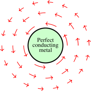
Figure 1: An axionic response $\boldsymbol{\zeta}=\zeta_{\theta}\hat{\boldsymbol{\theta}}$ (arrows) outside a charged conducting cylinder, shown in the cross section of the plane perpendicular to the cylinder.

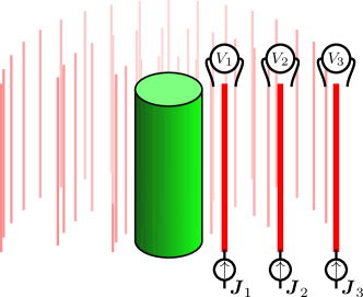
Figure 2: Emulating the $-\boldsymbol{\zeta}\times\boldsymbol{E}$ term using a conducting metal cylinder (green) surrounded by a radial array of wires (pink), with a few wires visually emphasised in order to clarify the setup. A series of voltmeters measure the radial electric fields (e.g. $V_{1}$, $V_{2}$, …) near each wire, and the resulting information is used to control a current source that drives currents along those wires (e.g. $\boldsymbol{J}_{1}\propto V_{1}/r$, $\boldsymbol{J}_{2}\propto V_{2}/r$, …). As a result these actively monitored and driven wires will act as a metamaterial, modifying the electromagnetic field as if a constitutive axionic response $\boldsymbol{\zeta}$ were present. As an alternative, one might imagine replacing the array of wires with an array of controllable high energy electron beams, since at sufficiently high energy the electrons will not be deflected significantly by a (relatively weak) background electromagnetic field.

IV.1 Outside a conducting cylinder

An example that could in principle be built consists of an infinite conducting metal cylinder, which enables us to avoid difficulties at $r=0$. The cylinder is charged in order to create a purely radial electric field ($E_{r}$) with no axial component ($E_{z}=0$), and then surrounded by an array of parallel wires used to implement the axionic response. With the cylinder and wires being oriented parallel to the $z$-axis, then for a cylinder of radius $r=r_{0}$, in this static case we can set

$$\boldsymbol{\zeta}=\frac{Z_{0}}{r}\ \hat{\boldsymbol{\theta}}\qquad\textup{and}\qquad\zeta_{t}=0$$ (33)

where $Z_{0}$ is a constant, as shown in figure 1. Here ($r$, $\theta$, $z$) are the cylindrical coordinates and ($\hat{\boldsymbol{r}}$, $\hat{\boldsymbol{\theta}}$, $\hat{\boldsymbol{z}}$) the corresponding orthonormal vectors. However, this does not satisfy (27) since

$$\nabla\times\boldsymbol{\zeta}=\frac{1}{r_{0}}\,\delta(r-r_{0})\,\hat{\boldsymbol{z}},$$ (34)

but of course (27) is required only inside bulk materials. Fortunately, on the boundary of the cylinder, $\boldsymbol{E}$ is along $\hat{\boldsymbol{r}}$ so (26), and hence the conservation of charge is satisfied after all.

A crucial point that separates our CMCR from the standard constitutive relations is that in this situation $\boldsymbol{\zeta}$ cannot be the gradient of any field as in (28); thus the standard constitutive relations cannot describe this. Although locally we can set ${\kappa}_{\textup{ax}}=Z_{0}\theta$, globally $\theta$ is not single valued and continuous; thus it would be impossible to model such a material using the traditional Maxwell’s equations, no matter what constitutive relations were used.

However, with our CMCR we can emulate the axionic response (33). This is done by first measuring the radial electric field at each point, and then using that information to specify a current source $-\boldsymbol{\zeta}\times\boldsymbol{E}$ along $z$-directed wires. As shown in figure 2, a radially directed electric field could – by means of an active measurement and current generation process – give rise to the necessary axial current, as per (25). Naturally, if the charge on the cylinder varies over time, such variation will need to be on much slower timescales than the reaction time of the active measurement and current generation processes in order to remain causal Kinsler (2010). An alternative method of emulating an axionic response dynamically, using a mechanical substructure, is suggested in section VI.1.

For the angular axionic response discussed here, we can solve the local axionic media equations (24), (25) with a static radial solution given by

$$\boldsymbol{E}(r) =\left(G_{1}r^{-1+\alpha}+G_{2}r^{-1-\alpha}\right)\,\hat{\boldsymbol{r}},$$ (35)

$$\text{and}\qquad\boldsymbol{B}(r) =\alpha Z\varepsilon^{-1}\left(G_{1}r^{-1+\alpha}-G_{2}r^{-1-\alpha}\right)\,\hat{\boldsymbol{\theta}},$$

where $\alpha=Z_{0}^{2}\,\mu\,\varepsilon^{-1}$.

IV.2 Toroidal universes and periodic lattices, with charge.

The toroidal universe imagined here is one in which the spatial $x$, $y$ and $z$ coordinates are periodic, with $x\to x+L_{x}$, $y\to y+L_{y}$ and $z\to z+L_{z}$. This situation is also compatible with an infinitely periodic system, whose physical properties are periodic, even if the coordinates themselves are not. In such a toroidal universe the standard Maxwell’s equation (6) in concert with the divergence theorem implies that the total charge is zero:

$$\int_{0}^{L_{x}}dx \int_{0}^{L_{y}}dy\int_{0}^{L_{z}}dz~{}~{}\rho=\iiint_{V}\rho\,dx\,dy\,dz$$ (36)

$$=\iiint_{V}\left(\nabla\cdot\boldsymbol{D}\right)~{}~{}dx\,dy\,dz=\iint_{\partial V}\boldsymbol{D}\cdot d\boldsymbol{S}=0$$

where $V$ is the 3-torus and $\partial V$ is its boundary. However, since a torus does not possess a boundary (i.e. $\partial V=\emptyset$), any integral over it is zero – i.e. there can be no net charge on the torus. In the periodic counterpart to (36), the torus maps onto each cell in the periodic lattice, and since the contributions from opposite cell boundaries are equal but have opposite orientations, they exactly cancel, and again no net charge is ensured.

By contrast, our generalised CMCR gives a different substitution for the charge, i.e. according to (14). The total charge is then given by

$$\int_{0}^{L_{x}}dx \int_{0}^{L_{y}}dy\int_{0}^{L_{z}}dz~{}~{}\rho$$ (37)

$$=\int_{0}^{L_{x}}dx\int_{0}^{L_{y}}dy\int_{0}^{L_{z}}dz~{}~{}\left({{\Psi}}^{E}_{\rho}\!\left\langle\boldsymbol{E}\right\rangle+{{\Psi}}^{B}_{\rho}\!\left\langle\boldsymbol{B}\right\rangle\right),$$

which depends on ${{\Psi}}^{E}_{\rho}$ and ${{\Psi}}^{B}_{\rho}$, and can therefore be non-zero.

The result has practical implications when considering any periodic system of size ($L_{x}$, $L_{y}$, $L_{z}$), and determining its Floquet modes, for example using a numerical electromagnetic solver. The approach using the standard EMCR yeilds (36), which insists that the total charge on the lattice is zero. However, if the charge is not zero, then we must either abandon (a) the claim that the system is periodic, or (b) the concept of a meaningful $\boldsymbol{D}$ in the lattice, and choose to use the CMCR proposed here.

We now show that a periodic solution with net free charge is possible, in the following static case based on our CMCR. Consider a toroidal space, or an equivalent infinitely periodic one where the coordinates $x$, $y$, and $z$ range over (or are periodic on) lengths $L_{x}$, $L_{y}$, and $L_{z}$. Assume that the free charge density has no $z$ dependence and is $\rho(x,y)$, there is no free current density so that $\boldsymbol{J}={\boldsymbol{0}}$, that the axionic response consists solely of a homogeneous $\zeta_{z}$ component. In this situation the electric field components that exist are ${E}_{x}$ and ${E}_{y}$, so that $\boldsymbol{E}=\hat{\boldsymbol{x}}{E}_{x}(x,y)+\hat{\boldsymbol{y}}{E}_{y}(x,y)$. The only magnetic field contribution will be generated by the axionic response $\zeta_{z}$, and so consist only of ${B}_{z}$, so that $\boldsymbol{B}=\hat{\boldsymbol{z}}{B}_{z}(x,y)$.

The source free axionic vacuum equations (24) and (28) then reduce to just three non-zero contributions

$$\partial_{x}{E}_{x}+\partial_{y}{E}_{y}-\zeta_{z}{B}_{z} =\rho,$$ (38)

$$\partial_{y}{B}_{z}+\zeta_{z}{E}_{y} =0,$$ (39)

$$-\partial_{x}{B}_{z}-\zeta_{z}{E}_{x} =0.$$ (40)

For non-zero $\zeta_{z}$, (39) and (40) can be substituted into (38) to give

$$-\partial_{x}^{2}{B}_{z}-\partial_{y}^{2}{B}_{z}-\zeta_{z}^{2}{B}_{z} =\zeta_{z}{\rho}.$$ (41)

A periodic $\rho(x,y)$ can be written as a Fourier series where

$$\rho(x,y) =\sum_{nm}{\rho}_{nm}\cos\left(\frac{n\pi}{2L_{x}}x\right)\cos\left(\frac{m\pi}{2L_{y}}y\right),$$ (42)

where the sums are over $n,m\in\{0,1,2,\ldots,\infty\}$ and the coordinate range is centred about the origin.

Since the system is periodic, ${B}_{z}$ is also periodic, and can also be written as a Fourier series

$${B}_{z}(x,y) =\sum_{nm}b_{nm}\cos\left(\frac{n\pi}{2L_{x}}x\right)\cos\left(\frac{m\pi}{2L_{y}}y\right).$$ (43)

Now we can use (41) to relate the ${\rho}_{nm}$ coefficients to the $b_{nm}$, i.e.

$$\left[\left(\frac{n\pi}{2L_{x}}\right)^{2}+\left(\frac{m\pi}{2L_{y}}\right)^{2}-\zeta_{z}^{2}\right]b_{nm} =\zeta_{z}{\rho}_{nm}$$ , (44)

and this allows us to easily determine each of the $b_{nm}$ from any given $\rho(x,y)$. Further, since any electric field component ${E}_{i}(x,y)$ must also be periodic, with Fourier components $e_{i,nm}$, then we also have from (39) and (40)

$$e_{x,nm} =\frac{1}{\zeta_{z}}\frac{n\pi}{2L_{x}}b_{nm},\quad\textrm{and}\quad e_{y,nm} =\frac{1}{\zeta_{z}}\frac{m\pi}{2L_{y}}b_{nm}.$$ (45)

We also need to satisfy both of (4) and (5). We already have $\nabla\cdot\boldsymbol{B}=0$ because ${B}_{z}$ depends only on $x,y$. This leaves the condition $\nabla\times\boldsymbol{E}=0$, i.e. that

$$\frac{m\pi}{2L_{y}}e_{x,nm} =\frac{n\pi}{2L_{x}}e_{y,nm},$$ (46)

which can be converted into a condition not only on $b_{nm}$ but also the charge distribution parameters $\rho_{nm}$; fortunately, a back substitution reveals that this is already satisfied.

Note that the interesting case here is when the net charge on the system is non-zero, which occurs solely when ${\rho}_{00}$ is non-zero. Indeed, the total charge on the torus – or one element in the periodic lattice – is simply $\rho_{\textrm{total}}={\rho}_{00}L_{x}L_{y}L_{z}$. Here the charge density, and hence the fields, are constant, has a field solution trivially obtained from (38) where $\boldsymbol{E}={\boldsymbol{0}}$ and $\boldsymbol{B}=-\hat{\boldsymbol{z}}\left(\rho/\zeta_{z}\right)$. Thus although there is a charge on the torus, there is no electric field from that charge; there is only an axionically-induced magnetic field whose field lines form (topologically allowed) loops.

In the more general solutions, we can see that the additional coupling between the electric and magnetic fields permitted by the presence of the axionic response allows a finite charge to be supported in the system. Consider each effect in turn: the free charge creates an electric field, then that electric field causes the axionic response to generate a polarization current, then this polarization current in turn creates a magnetic field. Finally, this magnetic field causes the axionic response to (also) create a polarization charge; and we find that this exactly counteracts the free charge.

V Examples

In this section we consider situations involving conventional media with additional constitutive properties that match the axionic responses described above. We will call these axionic response materials, and it is important to note that they have a vacuum contribution (or a conventional and homogeneous $\varepsilon$ and $\mu$) in their constitutive properties as well as the added axionic response. In what follows, remember that these are constitutive properties, and are not the result of coupling Maxwell’s equations to an external axion particle field.

V.1 Homogeneous case: longitudinal waves

The propagation of electromagnetic fields in media with an axion-like response has been an area of interest for some time Itin (2008); Visinelli (2013), particularly with regard to its symmetry properties and axionic dispersion relations. A starting point of a homogeneous axionic response material with all 4 constitutive terms being non-zero contains a large number of interesting cross-couplings between the $\boldsymbol{E}$ and $\boldsymbol{B}$ fields, leading to a range of new behaviours. Here, however we will highlight one interesting feature – namely that propagating EM fields in a homogeneous medium, with isotropic $\varepsilon$ and $\mu$, need no longer be purely transverse.

Starting with Maxwell’s equations (4), (5) and the source free axionic vacuum equations (24) and (28) we have

$$\begin{gathered}\nabla\cdot\boldsymbol{B}=0,\qquad\nabla\times\boldsymbol{E}+\partial_{t}{\boldsymbol{B}}={\boldsymbol{0}},\\ \varepsilon_{0}\nabla\cdot\boldsymbol{E}+\boldsymbol{\zeta}\cdot\boldsymbol{B}=0,\\ \mu^{-1}_{0}\nabla\times\boldsymbol{B}-\varepsilon_{0}\partial_{t}{\boldsymbol{E}}-\boldsymbol{\zeta}\times\boldsymbol{E}-\zeta_{t}\boldsymbol{B}={\boldsymbol{0}}.\end{gathered}$$ (47)

We can show that the existence of the axionic response terms enables the propagation of EM waves with a longitudinal component, as depicted on figure 3. Although achievable with the aid of artificial functional materials Gratus et al. (2017); Boyd et al. (2018a, b), or in an ordinary anisotropic (birefringent) medium, here we can do this with simple homogeneous constitutive properties.

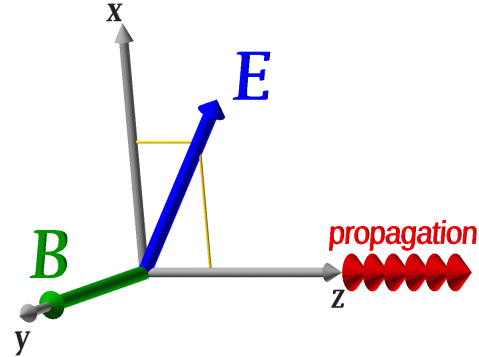
Figure 3: An EM wave propagating in the $\hat{\boldsymbol{z}}$ direction has its electric field vector $\boldsymbol{E}$ (thick blue arrow) rotated forwards in the ${\hat{\boldsymbol{x}}}{-}{\hat{\boldsymbol{z}}}$ plane by an axionic perturbation to the propagation medium; in the case shown the magnetic field vector $\boldsymbol{B}$ (thick green arrow) remains transverse. The propagation direction $\boldsymbol{k}$ is indicated with multiple arrowheads (red) for clarity. The thin arrows indicate the coordinate axes.

For example for a wave travelling in the $\hat{\boldsymbol{z}}$-direction satisfying the dispersion relations

$$\omega^{2}+\zeta_{y}^{2}\varepsilon_{0}^{-2}-c^{2}k^{2} =0,$$ (48)

and compatible with constraints on the axionic response

$$\omega\zeta_{z}+k\zeta_{t} =0,\qquad\textup{and}\qquad\zeta_{x}=0.$$ (49)

By direct substitution we see the propagating electromagnetic field given by

$$\boldsymbol{E} ={E}_{0}\omega\cos\left(\omega t-kz\right)\hat{\boldsymbol{x}}-{E}_{0}\frac{\zeta_{y}}{\varepsilon_{0}}\sin\left(\omega t-kz\right)\hat{\boldsymbol{z}},$$ (50)

$$\boldsymbol{B} ={E}_{0}k\cos\left(\omega t-kz\right)\hat{\boldsymbol{y}}.$$ (51)

is a solution to Maxwell’s equations in a vacuum axionic response material (47). Note here how the homogeneous $\zeta_{y}$ axionic response material still supports the propagation whilst having rotated the electric field orientation forward, away from a purely transverse direction.

V.2 Inhomogeneous case: Static solutions

Here we consider two static cases based on cylindrical symmetry. These are based primarily on a combination of a thin cylindrical shell which has radius $R_{c}$ and thickness $T$, and a thin wire with radius $R_{w}$, as depicted on figure 4. They are made of a vacuum augmented with an axionic response of the kind described above. Although we would like to treat each of the 4 axionic components separately, it turns out that only the $z$-directed ($\zeta_{z}$) and the $t$-directed ($\zeta_{t}$) are sufficiently interesting whilst still allowing a straightforward discussion – the case where radial $\zeta_{r}$ is non-zero is very simple, the case where angular $\zeta_{\theta}$ is non-zero is rather complicated.

The cylindrical symmetry here means that the modulation function for the axionic wire and shell properties depends only on $r$, and is a sum of offset step functions ${\mathfrak{H}}$. For a wire of radius $R_{w}$ the modulation (density) function $W(r)$ is

$$W(r) =W_{w}(r)+W_{c}(r)$$

$$=\tfrac{1}{\pi R_{w}^{2}}{\mathfrak{H}}(R_{w}-r)$$

$$\quad+\tfrac{1}{\pi R_{w}^{2}}\left[{\mathfrak{H}}(r-R_{c}+\tfrac{T}{2})-{\mathfrak{H}}(r-R_{c}-\tfrac{T}{2})\right].$$ (52)

Here this modulation function has been normalised to compensate for the effect of the wire’s cross-sectional area. In the examples below, there are only the fields $\boldsymbol{E}$ and $\boldsymbol{B}$, and two types of sources. There is free (source) charge ${C}$ and free (source) current ${\boldsymbol{J}}$; in addition there are polarization (charge and current) sources. The polarization sources are those induced in the medium by the presence of an $\boldsymbol{E}$ or $\boldsymbol{B}$ field acting on the axionic response.

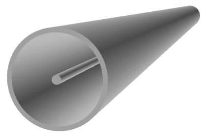
Figure 4: The wire and shell system represented by (52) with a wire of radius $R_{w}=1$, and a shell centred at $R_{c}=10$ with thickness $T=1$. The wire and cylindrical shell lie along the $z$ axis.

V.2.1 Free charge and axial axionic response $\zeta_{z}$

Here we take the wire and cylindrical shell to consist of an axionic response material with only $\zeta_{z}(r)$ being non-zero. This can be derived from a ${\kappa}_{\textup{ax}}(r,\theta,z,t)$ with an appropriate $r$-dependent modulation $W(r)$ of a linear increase along the axis $z$;

$${\kappa}_{\textup{ax}}(r,z)=\zeta_{z}W(r)z,$$ (53)

where $W(r)$ is zero everywhere but in the wire and shell. However, somewhat inconveniently, this ${\kappa}_{\textup{ax}}(r,z)$ also has an $r$ derivative, and so along with our desired $\zeta_{z}$ properties we also get a non-zero and $z$-dependent $\zeta_{r}$ on the surfaces of the wire and shell.

If we write just the combinations that are potentially non-zero, then with $\boldsymbol{B}={B}_{r}\hat{\boldsymbol{r}}+{B}_{\theta}\hat{\boldsymbol{\theta}}+{B}_{z}\hat{\boldsymbol{z}}$ and $\boldsymbol{E}={E}_{r}\hat{\boldsymbol{r}}+{E}_{\theta}\hat{\boldsymbol{\theta}}+{E}_{z}\hat{\boldsymbol{z}}$, the static constitutive relations in the medium are

$$\varepsilon\nabla\cdot\boldsymbol{E}-W(r)\zeta_{r}{B}_{r}-W(r)\zeta_{z}{B}_{z} =W(r){C}$$ (54)

$$\frac{1}{\mu}\nabla\times\boldsymbol{B}+W(r)\left(\zeta_{r}\hat{\boldsymbol{r}}+\zeta_{z}\hat{\boldsymbol{z}}\right)\times\boldsymbol{E} =W(r){\boldsymbol{J}}.$$ (55)

Note the nature of the $\zeta_{r}$ surface terms in these two equations, and, in particular, that (a) if the magnetic field has no radial component, and (b) if the electric field remains purely radial, they will have no effect. Because of our construction, the radial symmetry guarantees both a radial electric field, and an enforced non-radial magnetic field. This means the $\zeta_{r}$ surface terms play no role in the following calculation; but if the symmetry was broken and they did, to first order they would induce surface charges and currents on the wire and shell.

These symmetry restrictions reduce the above equations to simpler ones; and also mean that the other Maxwell equations, namely (4) and (5) are automatically satisfied. The first equation is for the radial electric field ${E}_{r}$ given the presence of the free charge line density ${C}$ and an axial magnetic field ${B}_{z}$:

$$\varepsilon r^{-1}\partial_{r}\left[r{E}_{r}\right] =W_{w}(r){C}+W(r)\zeta_{z}{B}_{z},$$ (56)

where the second RHS term can be interpreted as a polarization charge density induced by the action of the free fields on the axionic response of the medium. The second equation is for the axial magnetic field ${B}_{z}$ under the influence of the radial electric field ${E}_{r}$:

$$\mu^{-1}\partial_{r}{B}_{z} =-W(r)\zeta_{z}{E}_{r},$$ (57)

where the RHS can be interpreted as a polarization current density induced by the action of the free fields on the axionic response.

These two equations can be combined, resulting in inhomogeneous Bessel’s equations of order $\nu=0$ for ${B}_{z}$ and order $\nu=1$ for ${E}_{r}$. With $\bar{r}=W\zeta_{z}r$ and a suitably scaled charge density $\bar{C}$, we have

$$\bar{r}^{2}\partial_{\bar{r}}^{2}{B}_{z}+\bar{r}\partial_{\bar{r}}{B}_{z}+\bar{r}^{2}{B}_{z} =-\bar{r}^{2}\bar{C},$$ (58)

$$\bar{r}^{2}\partial_{\bar{r}}^{2}{E}_{r}+\bar{r}\partial_{\bar{r}}{E}_{r}+\left[\bar{r}^{2}-1\right]{E}_{r} =0.$$ (59)

Note in particular that such behaviour emphasises again the difference between our CMCR response and the standard tensorial EMCR one. Standard EMCRs only allow coupling to axionic effects to occur at boundaries, but here we see the effects of the axionic response present in a homogeneous system (i.e. inside the wire and/or shell).

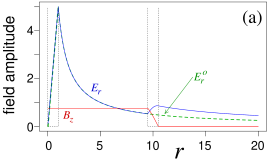
Figure 5: The fields in a wire and shell system in scaled units with $\varepsilon=1,\mu=1$, and $\zeta_{z}=1$, with line charge density ${C}=1$ on the wire. The wire has a radius $R_{w}=1$ and the shell is centred at $R_{c}=10$ with thickness $T=1$. The electric field ${E}_{r}$ is in blue, and the magnetic field ${B}_{z}$ is in red. The green dashed curve is the radial electric field ${E}_{r}^{o}$ obtained for the same charge density distribution in non-axionic materials. The upper panel (a) shows an alternate simpler case where the wire is charged but has no axionic response (i.e. its modulation function differs from (52)), whereas the lower panel (b) shows results for a both charged and axionic wire (and is consistent with (52)).

We now numerically solve (56) and (57) in order to give a qualitative sense of the axionic effects. Solution is straightforward, the only constraint being that we must pick an initial ${B}_{z}$ value at $r=0$ that results in ${B}_{z}=0$ outside the shell. We achieve this using a simple iterative process for zero-finding that converges to the right answer.

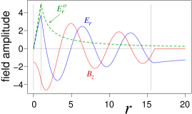
Figure 6: The fields in a wire embedded inside a thick cylinder, in scaled units with $\varepsilon=1,\mu=1$, and $\zeta_{z}=1$, with line charge density ${C}=1$ on the wire. The wire has a radius $R_{w}=1$ and the shell is centred at $R_{c}=8.5$ with thickness $T=15$. The electric field ${E}_{r}$ is in blue, and the magnetic field ${B}_{z}$ is in red. The green dashed curve is the radial electric field ${E}_{r}^{o}$ obtained for the same charge density distribution in non-axionic materials. The Bessel-like nature of the fields under the influence of this axionic material can be clearly seen. Notably, even though the oppositely-signed ${B}_{z}$ inside the wire acts to suppress the effective charge density there, the field oscillations here enhance the electric field strength outside the shell, whilst also swapping its sign.

A typical result is shown on figure 5. Here the axionic effect is fairly strong, which enables the character of the modifications from the non-axionic result to be easily seen. In figure 5(a), where there is no axionic response in the wire, we see that the ${E}_{r}$ matches that for an ordinary charged rod until it reaches the shell. In the shell the ${E}_{r}$ induces a circulating polarization current, which generates the constant ${B}_{z}$ inside the shell and wire. As the ${B}_{z}$ falls to zero across the shell, it induces a polarization charge, which enhances the electric field.

In figure 5(b), the axionic response in the wire leads to an extra inverted parabolic behaviour for ${B}_{z}$, and this increased ${B}_{z}$ induces a polarization charge which enhances the electric field. However, note that increasing $\zeta_{z}$ further can push the results into a regime where axionic effects triggered by the charge density dominate, and the electric field can even change sign.

With sufficient distance in which to accumulate these axionic response effects further, we see more complicated behaviour. In figure 6 we see how if the shell is thick and there is no gap between it and the wire, an oscillatory Bessel function behaviour manifests itself, in line with (58) and (59).

V.2.2 Free current and time-directed axionic response: $\zeta_{t}$

Here we take the wire and cylindrical shell to consist of an axionic response material with only $\zeta_{t}(r)$ being non-zero; note that despite the different physics, this derivation follows very similar steps to the previous one. This can be derived from a ${\kappa}_{\textup{ax}}(r,\theta,z,t)$ with an appropriate $r$-dependent modulation $W(r)$ of a linear increase in time $t$;

$${\kappa}_{\textup{ax}}(r,t)=\zeta_{t}W(r)t,$$ (60)

where $W(r)$ is zero everywhere but in the wire and shell. However, somewhat inconveniently, this ${\kappa}_{\textup{ax}}(r,t)$ does have an $r$ derivative, and so along with our desired $\zeta_{t}$ properties we also obtain a non-zero and $t$-dependent $\zeta_{r}$ on the surfaces of the wire and shell.

If we write down just the potentially non-zero combinations, the static constitutive relations in the medium are

$$\varepsilon\nabla\cdot\boldsymbol{E}-W(r)\zeta_{r}\cdot{B}_{r} =W(r){C},$$ (61)

$$\frac{1}{\mu}\nabla\times\boldsymbol{B}+W(r)\left(\zeta_{r}\hat{\boldsymbol{r}}\right)\times\boldsymbol{E}$$

$$+W(r)\zeta_{t}\boldsymbol{B} =W(r){\boldsymbol{J}}.$$ (62)

Note the nature of the $\zeta_{r}$ surface terms in these two equations, and in particular that if the electric field remains purely radial, they will have no effect. Because of our construction, there is no electric behaviour in this system, and even if one somehow appeared, the radial symmetry would guarantee a concommitantly radial electric field. This means that the $\zeta_{r}$ surface terms play no role in the following calculation; but if the symmetry was broken and they did, they would induce surface charges and currents on the wire and shell.

These symmetry restrictions reduce the above equations to simpler ones; and also mean that the other Maxwell equations, namely (4) and (5) are automatically satisfied. The first equation is for the angular magnetic field ${B}_{\theta}$ resulting from the current density ${J}_{z}$ and any axial magnetic field ${B}_{z}$:

$$\mu^{-1}r^{-1}\partial_{r}\left[r{B}_{\theta}\right] =W(r){J}_{z}-W(r)\zeta_{t}{B}_{z},$$ (63)

where the second RHS term can be interpreted as a polarization current density induced by the action of the axial magnetic field on the axionic response of the medium. The second equation is for the axial magnetic field ${B}_{z}$ under the influence of the angular magnetic field ${B}_{\theta}$:

$$\mu^{-1}\partial_{r}{B}_{z} =-W(r)\zeta_{t}{B}_{\theta},$$ (64)

where the RHS term can be interpreted as a polarization current density induced by the action of the angular magnetic field on the axionic response.

These two equations can be combined, resulting in inhomogeneous Bessel’s equations of orders $\nu=0$ and $\nu=1$ for ${B}_{z}$ and ${B}_{\theta}$ respectively. With $\bar{r}=W\zeta_{t}r$ and a suitably scaled current $\bar{J}_{z}$, we have

$${\bar{r}}^{2}\partial_{\bar{r}}^{2}{B}_{z}+{\bar{r}}\partial_{\bar{r}}{B}_{z}+{\bar{r}}^{2}{B}_{z} ={\bar{r}}^{2}\bar{{J}}_{z},$$ (65)

$${\bar{r}}^{2}\partial_{\bar{r}}^{2}{B}_{\theta}+{\bar{r}}\partial_{\bar{r}}{B}_{\theta}+\left[{\bar{r}}^{2}-1\right]{B}_{\theta} =0.$$ (66)

Note that solutions for this system are mathematically identical to those presented in the previous subsection, for an $\zeta_{z}$ response. This can be seen by inspection of (63) and (64), and comparison with (56) and (57); the differences being solely the replacement of ${E}_{r}$ with ${B}_{\theta}$, of $\varepsilon$ with $1/\mu$, a sign on the axionic term, and replacing the charge density $C$ with ${J}_{z}$.

VI Other Topics

VI.1 Metamechanical axionic response

An interesting question is whether or not it is possible to design a metamaterial unit cell which can generate an axionic response of the kinds discussed here. Broadly speaking, there are two sorts of axionic response, those that generate charge (see (24)) and those that generate current (see (25)). Since it is hard to generate a free charge from nowhere, or turn on and off some mechanism for isolating that charge, it is easiest to focus on current generating axionic responses.

Since the axionic response is outside the scope of standard electromagnetism, we will utilise concepts from the area of mechanical metamaterials Surjadi et al. (2019); Yu et al. (2018), albeit ones driven by applied electromagnetic fields, and which – with the addition of moving charged elements, can generate currents. It is the mechanical movement and couplings of the metamaterial component that create constitutive properties of the necessary orientation for an axionic response.

The metamaterial unit cell concept shown in figure 7 depicts a mechanism intended to create the axionic response where an electric field applied across the page (e.g. along $\hat{\boldsymbol{x}}$) generates a vertical current (oriented along $\hat{\boldsymbol{y}}$). Whilst this suffices for selecting the appropriate axionic response orientations with respect to the field, this is not the complete picture. As with the great majority of metamaterial schemes, this is (a) a dynamic response suitable for oscillating fields only, and (b) will typically only generate the desired response current with a phase offset to the driving field. Further, it will also generate a side effect current (along $\hat{\boldsymbol{x}}$), and of itself generate a background dipolar/quadrupolar electric field. Nevertheless, if the driving electric field is strong, and the detector charges $q_{b}$ are weak compared to the response ones $q_{r}$, and the mechanical system oscillates and is driven at the correct frequency, the system can function as an axionic response.

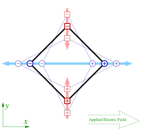
Figure 7: Diagram of a current-generating axionic response $\zeta_{z}\hat{\boldsymbol{z}}$, based on a diamond shape that stretches (or shrinks) in $x$ whilst simultaneously contracting (or expanding) in $y$. When an oscillating electric field ${E}_{x}$ is applied, the “detector” charges (blue circles) are pulled apart (or pushed together) horizontally, so that the “response” charges (red squares) are moved together (apart) vertically. The $y$-direction current produced by those moving response charges is the axionic response. Not shown are the mechanisms that return the system to a default shape when the applied field is removed; for a construction with sufficiently flexible corners, this could be provided by the elastic properties of the material.

For a minimal material providing such properties, we assume a model response dynamics, where $x$ is the charge displacement, $v$ is the speed of motion of any corner, $K$ the restoring force constant, and $m$ the effective mass of the structure, of

$$\partial_{t}x =v$$ (67)

$$\partial_{t}v =-Kx-\gamma v-\frac{2q_{b}}{m}{E}_{x}$$ (68)

$$\textrm{i.e.}\qquad\partial_{t}^{2}v =-Kv-\gamma\partial_{t}v-\frac{2q_{b}}{m}\partial_{t}{E}_{x}$$ (69)

$$\textrm{or}\qquad\partial_{t}^{2}{J}_{y} =-K{J}_{y}-2q_{r}\gamma\partial_{t}v-\frac{4q_{r}q_{b}}{m}\partial_{t}{E}_{x},$$ (70)

since ${J}_{y}=2q_{r}v$. Here, $\gamma$ represents frictional losses in the mechanical oscillator.

In the quasistatic case with ${E}_{x}$ oscillating at a frequency $\omega_{0}$, and with negligible losses, we have

$$\hat{\boldsymbol{y}}{J}_{y} =\hat{\boldsymbol{z}}\left[\frac{\omega_{0}}{K+\imath\gamma\omega_{0}-\omega_{0}^{2}}\frac{4q_{r}q_{b}}{m}\right]\times\hat{\boldsymbol{x}}{E}_{x},$$ (71)

which means that

$${\zeta_{z}} =\frac{\omega_{0}}{K+\imath\gamma\omega_{0}-\omega_{0}^{2}}\frac{4q_{r}q_{b}}{m}.$$ (72)

Note that (72) is frequency dependent, and is the dispersion relation for the axionic response. As the response is derived from the causal dynamical model of (67), (68) it automatically satifies the Kramers-Kronig relations Kinsler (2011); and in some suitably narrowband limit could be approximated as being dispersionless.

Note that at the expense of additional complication, the unwanted current due to the detector charges could be (partly) cancelled by stacking the element of figure 7 with the complementary “auxetic” one of figure 8. In the auxetic Yu et al. (2018) cell, the shape expands simultaneously in $x$ and $y$; as a result, with (blue) detector charges of reversed sign (as shown), you can cancel the side-effect detector-charge currents with each other.

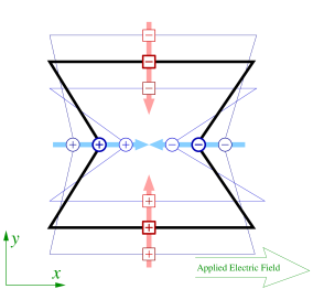
Figure 8: Diagram of an auxetic current-generating axionic response $\zeta_{z}\hat{\boldsymbol{z}}$, based on a shape whose core stretches (or shrinks) in $x$ whilst simultaneously expanding (or contracting) in $y$. When an oscillating electric field ${E}_{x}$ is applied, the “detector” charges (blue circles) are pushed together (or pulled apart) horizontally, so that the “response” charges (red squares) are moved together (or apart) vertically. The $y$-direction current produced by those moving response charges is the axionic response; notice that this response current is the same as in figure 7, whilst the current due to the detector charges is opposed. Not shown are the mechanisms that return the system to a default shape when the applied field is removed; for a construction with sufficiently flexible corners, this could be provided by the elastic properties of the material.

By placing elements of this kind radially around a conducting cylinder, with $\hat{\boldsymbol{x}}$ replaced with the radial direction $\hat{\boldsymbol{r}}$, and $\hat{\boldsymbol{y}}$ replaced with the angular direction $\hat{\boldsymbol{\theta}}$, we could envisage constructing a dynamical counterpart to an active, driven scheme such as that shown in figure 1; this is depicted in figure 9.

Figure 9: Metamaterial axionic response cells arranged radially about a conducting cylinder, to provide an axial axionic response $\zeta_{z}\hat{\boldsymbol{z}}$. This is rather like the concept of figure 1, except that to achieve the $\zeta_{\theta}\hat{\boldsymbol{\theta}}$ in that case the cells would need to be rotated about the radial axis and re-oriented into the $\hat{\boldsymbol{r}}\hat{\boldsymbol{z}}$ plane. The auxetic cells of figure 8 are used so that their proper orientation is clearer.

VI.2 Transformation Electromagnetics

There is much current interest in the concepts and applications of transformation optics in both space and spacetime Kinsler and McCall (2014a); Baev et al. (2015); Kinsler and McCall (2015); McCall et al. (2018), most notably involving various sorts of spatial and spacetime cloaking in free space Dolin (1961); Pendry et al. (2006); McCall et al. (2011); Gratus et al. (2016), against or on surfaces Li and Pendry (2008); Kinsler and McCall (2014b); Mitchell-Thomas et al. (2013), and at distance Lai et al. (2009).

It is worth investigating how such techniques are implemented under our new CMCR scheme. In transformation optics it is the optical metric where the cloaking or other transformation design is implemented; and it is important to note that that optical metric is distinct from the background physical (spacetime) metric Kinsler and McCall (2018); Fathi and Thompson (2016); Thompson and Fathi (2015).

For the constitutive model presented here, as detailed in our CMCR, (4), (5), (14), (15), we see that the metric (whether of the background spacetime or optical signals) does not explicitly appear. Instead its components and its derivatives are encoded within the components of the ${\Psi}$’s.

Since the operators (${{\Psi}}^{E}_{\rho}$, ${{\Psi}}^{B}_{\rho}$, ${{\Psi}}^{E}_{J}$, ${{\Psi}}^{B}_{J}$) contain derivatives, one idea to perform a transformation optics is to promote the partial derivatives $\partial_{i}$ in (16) to covariant derivatives $\nabla_{i}$. However this will not work because the operators (${{\Psi}}^{E}_{\rho}$, ${{\Psi}}^{B}_{\rho}$, ${{\Psi}}^{E}_{J}$, ${{\Psi}}^{B}_{J}$) are not tensors. Instead one should use the change of coordinates formula (115), (116) given in appendix A. For example, from this one can extract the components $({{\Psi}}^{E}_{\rho})^{i}$ using (95). In (116) we see that the non-axionic terms, i.e. those with two indices such as $({{\Psi}}^{E}_{\rho})^{0j}$, $({{\Psi}}^{E}_{\rho})^{ij}$, transform like tensor densities, albeit ones that can mix the non-axionic terms when performing a spacetime transformation. By contrast, (115) says that the transformation of the axionic terms has two contributions: one is the standard tensor transformation, and the other introduces the non-axionic terms multiplied by the derivative of the Jacobian matrix. This means that a medium which does not have an axionic response can be transformed into one which does. This is analogous to the way the Christoffel symbols, which in Minkowski spacetime with Cartesian coordinates are zero, can be transformed into non-zero values.

VI.3 Ohmic Resistance

Ohm’s law $\boldsymbol{J}=\sigma\boldsymbol{E}$ relates the current $\boldsymbol{J}$ through a conductor to the electric field $\boldsymbol{E}$ experienced by that conductor, with the proportionality between them being due to the conductivity $\sigma$. Here we are in particular looking for a constitutive relation giving us $\rho$ in terms of the electric field $\boldsymbol{E}$. Since – by conservation of charge – the charge at a point can be given by the time integral of the current, such a constitutive relation is obtained by inserting Ohm’s Law into this integral. Thus we have

$$\rho(t) =-\int_{t_{0}}^{t}\nabla\cdot\left(\sigma\boldsymbol{E}\right)\ dt^{\prime}+{\rho}(t_{0})$$ (73)

Since the CMCR equations (14) and (15) are a more general relationship between ($\boldsymbol{E}$, $\boldsymbol{B}$) and ($\rho$, $\boldsymbol{J}$) it is natural to ask if these avoid the problem of integral constitutive relations.

Consider a simple non-axionic isotropic homogeneous static medium with ${{\Psi}}^{E}_{J}\!\left\langle\boldsymbol{E}\right\rangle=\varepsilon\partial_{t}{\boldsymbol{E}}-\sigma\boldsymbol{E}$ and ${{\Psi}}^{B}_{J}\!\left\langle\boldsymbol{B}\right\rangle=\mu^{-1}\nabla\times\boldsymbol{B}$ so that (15) becomes

$$\mu^{-1}\nabla\times\boldsymbol{B}-\varepsilon\partial_{t}{\boldsymbol{E}} =\sigma\boldsymbol{E}+{\boldsymbol{J}}$$ (74)

where $\varepsilon$, $\mu$ and $\sigma$ are constants and $\boldsymbol{J}$ is the external current. In order to be consistent with (20), the other CMCR is given by

$$\varepsilon\nabla\cdot\boldsymbol{E}-\sigma\int\left(\nabla\cdot\boldsymbol{E}\right)dt ={\rho}\,.$$ (75)

Since this expression contains an integral clearly there do not exist any ${{\Psi}}^{E}_{\rho}$ and ${{\Psi}}^{B}_{\rho}$ such that (14) becomes (75).

However, we could decide to further extend the constitutive relations, so that the CMCR are also allowed to include second derivatives of ($\boldsymbol{E}$, $\boldsymbol{B}$) as well as first derivatives of $\rho$. In such a case, differentiating (75) with respect to time gives

$$\varepsilon\nabla\cdot\partial_{t}{\boldsymbol{E}}-\sigma\nabla\cdot\boldsymbol{E} ={\partial_{t}{\rho}}.$$ (76)

This means that such a “second order” extension to the CMCR would allow us to include a conductivity model of Ohmic current in the constitutive relations, just the standard constitutive relations can be extended by the addition of the conductivity parameter $\sigma$. In any such extension, there would be very many more allowed constitutive parameters than are considered here in our first order CMCR model.

VI.4 Poynting Vector

It is instructive to consider how these new axionic responses appear in the derivation of the electromagnetic energy flux equation, i.e. as applied to the Poynting vector Reitz et al. (1980); Kinsler et al. (2009). We have, using a standard vector identity and (25),  

$$\nabla\cdot \left(\boldsymbol{E}\times\boldsymbol{B}\right)$$

$$=-\boldsymbol{E}\cdot\left(\nabla\times\boldsymbol{B}\right)+\boldsymbol{B}\cdot\left(\nabla\times\boldsymbol{E}\right)$$

$$=-\boldsymbol{E}\cdot\mu\left(\varepsilon\partial_{t}{\boldsymbol{E}}-\boldsymbol{\zeta}\times\boldsymbol{E}-\zeta_{t}\boldsymbol{B}+\boldsymbol{J}\right){-}\boldsymbol{B}\cdot\partial_{t}{\boldsymbol{B}}$$

$$=-{\tfrac{1}{2}}\partial_{t}\left(\varepsilon\mu\boldsymbol{E}\cdot\boldsymbol{E}+\boldsymbol{B}\cdot\boldsymbol{B}\right)+\mu\boldsymbol{E}\cdot\left(\boldsymbol{\zeta}\times\boldsymbol{E}\right)$$

$$\qquad\qquad+\mu\zeta_{t}\boldsymbol{E}\cdot\boldsymbol{B}-\mu\boldsymbol{E}\cdot\boldsymbol{J}.$$

Hence

$$\partial_{t}\left({\tfrac{1}{2}}\varepsilon\boldsymbol{E}\cdot\boldsymbol{E}+{\tfrac{1}{2}}\mu^{-1}\boldsymbol{B}\cdot\boldsymbol{B}\right)+\nabla\cdot\left(\boldsymbol{E}\times\mu^{-1}\boldsymbol{B}\right)$$ (77)

$$\qquad=-\boldsymbol{E}\cdot\boldsymbol{J}+\zeta_{t}\boldsymbol{E}\cdot\boldsymbol{B},$$

where the only unconventional effect arises from the $\zeta_{t}$ term.

The conservation of momentum may also be derived as

$$\partial_{t}{\boldsymbol{p}} =\nabla\cdot\bar{\bar{{S}}}-\left(\boldsymbol{E}\cdot\boldsymbol{B}\right)\,\boldsymbol{\zeta}+\rho\,\boldsymbol{E}+\boldsymbol{J}\times\boldsymbol{B},$$ (78)

where the (Minkowski) electromagnetic momentum is

$${\boldsymbol{p}}=\varepsilon\,\boldsymbol{E}\times\boldsymbol{B},$$ (79)

and the electromagnetic stress tensor is

$$\left(\bar{\bar{{S}}}\right)_{ij} =\varepsilon\boldsymbol{E}_{i}\boldsymbol{E}_{j}+\mu^{-1}\boldsymbol{B}_{i}\boldsymbol{B}_{j}$$

$$\qquad\quad-\tfrac{1}{2}\left(\varepsilon\boldsymbol{E}\cdot\boldsymbol{E}+\mu^{-1}\boldsymbol{B}\cdot\boldsymbol{B}\right)\delta_{ij}.$$ (80)

The divergence of the stress tensor turns out to be

$$\left(\nabla\cdot\bar{\bar{{S}}}\right)_{j} =\partial^{i}\left(\bar{\bar{{S}}}\right)_{ij}$$

$$=\partial_{t}\left(\varepsilon\boldsymbol{B}\times\boldsymbol{E}\right)_{j}+\rho\boldsymbol{E}_{j}$$

$$\qquad\quad+\left(\boldsymbol{B}\times\boldsymbol{J}\right)_{j}+\boldsymbol{\zeta}_{j}\left(\boldsymbol{B}\cdot\boldsymbol{E}\right).$$ (81)

Here, as throughout this paper, we do not wish to consider the axionic terms ($\boldsymbol{\zeta}$, $\zeta_{t}$) as due to an axion particle field as in (1), but instead as background constitutive relations in the medium. Setting the external current to zero we see from (77) that energy is conserved only if $\zeta_{t}=0$. Similarly, a component of the ${\boldsymbol{p}}_{i}$ momentum is conserved only if the corresponding component of $\boldsymbol{\zeta}_{i}$ is zero. These observations are actually a consequence of existing work Gratus et al. (2012); Dereli et al. (2007), where it was shown that in the presence of a static background field, there is a conserved Noether current where there is a Killing symmetry that is simultaneously a symmetry of the metric and of the background field as it appears in the Lagrangian. In our case the background field appears as

$${\kappa}_{\textup{ax}}\,\boldsymbol{E}\cdot\boldsymbol{B}.$$ (82)

Thus time is a Killing symmetry of the Minkowski metric and a Lie symmetry of the axion current if $\zeta_{t}=\partial_{t}{\kappa}_{\textup{ax}}=0$, in this case the corresponding Noether current is energy. The results of Gratus et al. (2012) can also be used to predict the conservation of angular momentum if $\boldsymbol{\zeta}=\boldsymbol{\zeta}_{r}(r)\,\hat{\boldsymbol{r}}$ in the ($r$, $\theta$, $\phi$) coordinate system, and of angular momentum about the $z$-axis if $\boldsymbol{\zeta}=\boldsymbol{\zeta}_{r}(r,z)\hat{\boldsymbol{r}}+\boldsymbol{\zeta}_{z}(r,z)\hat{\boldsymbol{z}}$ in the cylindrical ($r$, $\theta$, $z$) case. The additional axionic $\zeta_{t}\boldsymbol{E}\cdot\boldsymbol{B}$ contribution to this EM energy flux equation acts comparably to the standard energy storage term (cf. (77)) or the work-done-on-charges term $\boldsymbol{E}\cdot\boldsymbol{J}$. Depending on the local fields, it acts as a source or sink for EM energy. In the usual case of an interaction with an axion particle field, this would be interpreted as a transfer of EM energy to or from those axions, where $\zeta_{t}$ can be identified with $\partial_{t}{\Xi}$. Here, it refers to energy transfer to or from the constitutive mechanism causing the axionic response.

VII Conclusion

We have presented a minimal extension to the standard constitutive relations for Maxwell’s equations, and have achieved this by combining the Maxwell-Ampère equation with the constitutive properties of an electromagnetic medium. This means that we eliminate the need for the excitation fields ($\boldsymbol{D}$, $\boldsymbol{H}$), and can permit a wider range of responses than the standard constitutive tensor approach. Although constraints mean that most likely only 4 new axionic (“axion-like”) parameters are permitted, these nevertheless represent media impossible to treat in the traditional approach, even if we allow inhomogeneity or dispersion. As such our new CMCR can be made to look like standard EMCR, but with the addition of extra axionic responses.

Notably, there are two cases when we cannot express our new axionic responses as an extension of standard EMCR, these being if we require the constitutive properties to be homogeneous, or in the case of non-trivial topology. In particular, homogeneous blocks of axionic materials represented using our CMCR appear as inhomogeneous materials if the representation is converted over to the standard EMCR. This is why the CMCR can represent axionic effects without relying – as is usually expected – on boundary effects.

This means that there are cases where it is advantageous – or even required – to write the axionic response in our way. These results are linked to related discoveries Gratus et al. (2019b) enabled by removing ($\boldsymbol{D}$, $\boldsymbol{H}$), such as non-conservation of charge in topologically non-trivial spaces, and the treatment of charges passing through wormholes. We also remarked on the possibility of there being an additional 16 more exotic constitutive parameters, for a grand total of 55 in all. If these exist, we either require additional new types of field and charge, or need to reconsider what we aim to represent by the excitation fields ($\boldsymbol{D}$, $\boldsymbol{H}$).

Another direction is to enumerate the plane eigenmodes of uniform media associated with our theory. Solving the eigen-problem of a conventional biaxial medium leads to the familiar self-intersecting Fresnel phase surface carrying four singular points Born and Wolf (2013). Recent generalisation from biaxial media to media with independent dielectric, magnetic, and magneto-electric tensors (a total of 20 material parameters) has been shown to give rise to a much richer Kummer surface, containing up to sixteen singular directions Favaro and Hehl (2014). With our proposed media containing a total of 55 parameters, even more contorted and exotic Fresnel phase surfaces are to be anticipated.

In future work we also aim to go beyond the minimal extension and theoretical discussion presented here. Our examples suggest a range of opportunities for further work based on these results in topological and periodic systems, in attempting a metamaterial implementation of the axionic response, or in extending the treatment to second order to treat Ohmic effects.

As a final remark, we wish to emphasise that this paper has only been written in standard vector calculus notation so as to make it more widely accessible. In fact, the CMCR minimal extension presented here can be written – and was originally written – much more succinctly in coordinate free notation using exterior forms. This is briefly presented in appendix C, where the equations do not include an explicit metric, and are therefore also consistent with a pre-metric formulation of electromagnetism Hehl and Obukhov (2003).

Appendix A In relativistic tensor notation

In both special and general relativity it is usual to combine the electromagnetic fields ($\boldsymbol{E}$, $\boldsymbol{B}$) into a single antisymmetric tensor $F_{ab}$ Post (1997). Here indices $a,b,\ldots$ span the range $\{0,1,2,3\}$, where for some coordinates $x^{a}$ we have that $x^{0}=t$; also we use indices $i,j,\ldots$ to represent only the spatial $\{1,2,3\}$. For some $F_{ab}$, we can extract the electric and magnetic fields with

$${E}_{i}=F_{0i}\qquad\textup{and}\qquad{B}_{\ell}=g_{\ell i}\epsilon^{ijk}F_{jk}..$$ (83)

where the extraction of the magnetic field ${B}_{\ell}$ requires both the Levi-Civita symbol $\epsilon^{ijk}$ and the metric $g_{\ell i}$.

In this notation Maxwell’s equations (4), (5) become

$$\partial_{a}F_{bc}+\partial_{b}F_{ca}+\partial_{c}F_{ab}=0,$$ (84)

which is automatically satisfied using the electromagnetic potential, which is a 4-vector ${A}_{a}$ such that

$$F_{ab} =\partial_{a}{A}_{b}-\partial_{b}{A}_{a}.$$ (85)

All the proofs for results in this appendix are given in detail in appendix B.

The advantage of using this relativistic notation is that the four separate CMCR operators (${{\Psi}}^{E}_{\rho}$, ${{\Psi}}^{B}_{\rho}$, ${{\Psi}}^{E}_{J}$, ${{\Psi}}^{B}_{J}$) can now be combined into a single CMCR operator $\Psi$. This operator takes the tensor $F_{ab}$ to the 4-vector density ${J}^{a}$ and so the two equations (14), (15) now combine into the single CMCR equation

$${{\Psi}}\!\left\langle F\right\rangle={J}$$ (86)

The operator ${{\Psi}}$ obeys the same three properties. It is linear, as in (18) and (19), so that

$${{\Psi}}\!\left\langle\alpha+\beta\right\rangle ={{\Psi}}\!\left\langle\alpha\right\rangle+{{\Psi}}\!\left\langle\beta\right\rangle\quad\textup{and}\quad{{\Psi}}\!\left\langle\lambda\,\alpha\right\rangle=\lambda\,{{\Psi}}\!\left\langle\alpha\right\rangle$$ (87)

where $\lambda\in{\mathbb{R}}$. It is also first order, as in (17)

$${{\Psi}}\!\left\langle{f}^{2}\,F\right\rangle =2{f}\,{{\Psi}}\!\left\langle{f}\,F\right\rangle-{f}^{2}\,{{\Psi}}\!\left\langle F\right\rangle,$$ (88)

for all scalar fields ${f}$ and all antisymmetric tensors $F$. Finally, the conservation of charge equation, corresponding to (21), is now written

$$\partial_{a}({{\Psi}}\!\left\langle F\right\rangle)^{a}=0\quad\textup{where}\quad F_{ab}=\partial_{a}{A}_{b}-\partial_{b}{A}_{a},$$ (89)

for all ${A}$.

•   All operators ${{\Psi}}$ which satisfy (87), (88) can be written

$$\left({{\Psi}}\!\left\langle F\right\rangle\right)^{a}=\tfrac{1}{2}{{\Psi}}^{abc}\,F_{bc}+\tfrac{1}{2}{{\Psi}}^{abcd}\left(\partial_{b}F_{cd}\right)$$ (90)

where clearly we demand

$${{\Psi}}^{a(bc)}=0\qquad\textup{and}\qquad{{\Psi}}^{ab(cd)}=0.$$ (91)

We can extract the components ${{\Psi}}^{abc}$ and ${{\Psi}}^{abcd}$ via

$${{\Psi}}^{abc} =\left({{\Psi}}\!\left\langle dx^{bc}\right\rangle\right)^{a}$$ (92)

$${{\Psi}}^{abcd} =\left({{\Psi}}\!\left\langle x^{b}\,dx^{cd}\right\rangle-x^{b}\,{{\Psi}}\!\left\langle dx^{cd}\right\rangle\right)^{a}$$ (93)

where $dx^{ab}$ is the antisymmetric tensor with components

$$(dx^{ab})_{cd} =\delta^{a}_{c}\,\delta^{b}_{d}-\delta^{a}_{d}\,\delta^{b}_{c}$$ (94)

It is trivial to see that ${{\Psi}}\!\left\langle F\right\rangle$ given by (90) obeys (87), (88). The converse is demonstrated in the appendix B, which also contains the proof of all the statements in this section. Thus without the charge conservation equation there are 120 components for ${{\Psi}}$.

•   The ${{\Psi}}^{abc}$ and ${{\Psi}}^{abcd}$ used above are simply a rewriting of the components of (${{\Psi}}^{E}_{\rho}$, ${{\Psi}}^{B}_{\rho}$, ${{\Psi}}^{E}_{J}$, ${{\Psi}}^{B}_{J}$). For example, we have

$$({{\Psi}}^{E}_{\rho})^{i}={{\Psi}}^{00i}\,,\quad({{\Psi}}^{E}_{\rho})^{0i}={{\Psi}}^{000i}\quad\textup{and}\quad({{\Psi}}^{E}_{\rho})^{ji}={{\Psi}}^{0j0i}.$$ (95)

•   Imposing charge conservation using (89) means that the components ${{\Psi}}^{abc}$ and ${{\Psi}}^{abcd}$ also obey

$$\partial_{a}{{\Psi}}^{abc} =0\,,$$ (96)

$${{\Psi}}^{(ab)c}+\partial_{d}{{\Psi}}^{d(ab)c} =0$$ (97)

$$\quad\textup{and}\quad{{\Psi}}^{(abc)d} =0.$$ (98)

•   In appendix B we show that (91) and (96)–(98) imply there are 4 independent components of ${{\Psi}}^{abc}$, corresponding to ($\boldsymbol{\zeta}$, $\zeta_{t}$) and 51 independent components of ${{\Psi}}^{abcd}$.

•   Clearly in the homogeneous case (96)–(98) reduce to

$${{\Psi}}^{(ab)c}=0\qquad\textup{and}\qquad{{\Psi}}^{(abc)d}=0$$ (99)

•   The null equivalent condition (30) relevant for the non-axionic extension terms becomes

$${\Psi}\to{\Psi}+\mathrel{\vbox{\offinterlineskip\halign{\hfil#\hfil\cr$\scriptscriptstyle\circ$\cr\kern 0.43057pt\cr${\Psi}$\cr}}}$$ (102)

where $\mathrel{\vbox{\offinterlineskip\halign{\hfil#\hfil\cr$\scriptscriptstyle\circ$\cr\kern 0.43057pt\cr${\Psi}$\cr}}}$ satisfies (87), (88); and in addition

$$\mathrel{\vbox{\offinterlineskip\halign{\hfil#\hfil\cr$\scriptscriptstyle\circ$\cr\kern 0.43057pt\cr${\Psi}$\cr}}}\!\left\langle F\right\rangle=0\quad\textup{where}\quad F_{ab}=\partial_{a}{A}_{b}-\partial_{b}{A}_{a}\quad\textup{for all}\quad{A}$$ (105)

In terms of components (105) becomes

$${\mathrel{\vbox{\offinterlineskip\halign{\hfil#\hfil\cr$\scriptscriptstyle\circ$\cr\kern 0.43057pt\cr${\Psi}$\cr}}}}\vphantom{{\Psi}}^{abcd}+{\mathrel{\vbox{\offinterlineskip\halign{\hfil#\hfil\cr$\scriptscriptstyle\circ$\cr\kern 0.43057pt\cr${\Psi}$\cr}}}}\vphantom{{\Psi}}^{acbd}-{\mathrel{\vbox{\offinterlineskip\halign{\hfil#\hfil\cr$\scriptscriptstyle\circ$\cr\kern 0.43057pt\cr${\Psi}$\cr}}}}\vphantom{{\Psi}}^{abdc}-{\mathrel{\vbox{\offinterlineskip\halign{\hfil#\hfil\cr$\scriptscriptstyle\circ$\cr\kern 0.43057pt\cr${\Psi}$\cr}}}}\vphantom{{\Psi}}^{adbc}=0.$$ (114)

•   In appendix B we show that (114) implies that ${\mathrel{\vbox{\offinterlineskip\halign{\hfil#\hfil\cr$\scriptscriptstyle\circ$\cr\kern 0.43057pt\cr${\Psi}$\cr}}}}\vphantom{{\Psi}}^{abcd}$ has 16 components.

•   Observe that although the components ${{\Psi}}^{abcd}$ transform as a tensor density under change of coordinates, the components ${{\Psi}}^{abc}$ do not. If $(x^{0},x^{1},x^{2},x^{3})$ and $({\hat{x}}^{0},{\hat{x}}^{1},{\hat{x}}^{2},{\hat{x}}^{3})$ are two coordinate systems then

$$\hat{{\Psi}}^{\hat{a}\hat{b}\hat{c}} =\Big{(}{{\Psi}}^{abc}~{}\frac{\partial{\hat{x}}^{\hat{b}}}{\partial x^{b}}~{}\frac{\partial{\hat{x}}^{\hat{c}}}{\partial x^{c}}+{{\Psi}}^{abcd}~{}\frac{\partial^{2}{\hat{x}}^{\hat{b}}}{\partial{x^{b}}\partial{x^{c}}}~{}\frac{\partial{\hat{x}}^{\hat{c}}}{\partial x^{d}}$$ (115)

$$\qquad\qquad\qquad+{{\Psi}}^{abcd}~{}\frac{\partial{\hat{x}}^{\hat{b}}}{\partial x^{c}}~{}\frac{\partial^{2}{\hat{x}}^{\hat{c}}}{\partial{x^{b}}\partial{x^{d}}}\Big{)}\frac{\partial{\hat{x}}^{\hat{a}}}{\partial x^{a}}~{}\frac{dx}{d{\hat{x}}}$$

and

$$\hat{{\Psi}}^{\hat{a}\hat{b}\hat{c}\hat{d}}={{\Psi}}^{abcd}~{}\frac{\partial{\hat{x}}^{\hat{b}}}{\partial x^{b}}~{}\frac{\partial{\hat{x}}^{\hat{c}}}{\partial x^{c}}~{}\frac{\partial{\hat{x}}^{\hat{d}}}{\partial x^{d}}~{}\frac{\partial{\hat{x}}^{\hat{a}}}{\partial x^{a}}~{}\frac{dx}{d{\hat{x}}},$$ (116)

where $\hat{{\Psi}}^{abc},\hat{{\Psi}}^{abcd}$ are the component with respect to $({\hat{x}}^{0},{\hat{x}}^{1},{\hat{x}}^{2},{\hat{x}}^{3})$ and $dx/d{\hat{x}}$ is the Jacobian. If higher order operators were to be considered, in an extension of our CMCR, they would lead to more unusual non tensorial changes of coordinates Gratus and Banaszek (2018).

Appendix B Proofs

Proof that (87), (88) implies (90), i.e. linearity.

Let $\lambda$ and $\mu$ be scalar fields. By considering ${{\Psi}}\!\left\langle(\lambda+\mu)^{2}F\right\rangle$ and ${{\Psi}}\!\left\langle(\lambda-\mu)^{2}F\right\rangle$ then we can show (88) implies

$${{\Psi}}\!\left\langle\lambda\mu\,F\right\rangle-\lambda{{\Psi}}\!\left\langle\mu\,F\right\rangle-\mu\,{{\Psi}}\!\left\langle\lambda\,F\right\rangle+\lambda\mu\,{{\Psi}}\!\left\langle F\right\rangle=0$$ (117)

Let $p$ be an event in spacetime with coordinates $(p^{0},p^{1},p^{2},p^{3})$ then expanding $F_{cd}$ about $p$ to second order gives

$$F_{cd} =F_{cd}|_{p}+(x^{b}-p^{b})\,(\partial_{b}F_{cd})|_{p}+$$

$$\qquad(x^{a}-p^{a})(x^{b}-p^{b})\,\alpha_{abcd}$$

where $\alpha_{abcd}$ a set of (indexed) scalar fields.

$$2\left({{\Psi}}\!\left\langle F\right\rangle\right)^{a}\big{|}_{p} ={{\Psi}}\!\left\langle(F_{cd}|_{p})\,dx^{ab}\right\rangle\big{|}_{p}$$

$$\qquad+{{\Psi}}\!\left\langle(x^{c}-p^{c})\,(\partial_{c}F_{cd})|_{p}\,dx^{ab}\right\rangle\big{|}_{p}$$

$$\qquad+{{\Psi}}\!\left\langle(x^{c}-p^{c})(x^{d}-p^{d})\,\alpha_{abcd}\right\rangle\big{|}_{p}$$

Now using (93) and (87) we have

$$\left({{\Psi}}\!\left\langle(F_{cd}|_{p})\,dx^{cd}\right\rangle\right)^{a}\big{|}_{p} =(F_{cd}|_{p})\,\left({{\Psi}}\!\left\langle dx^{cd}\right\rangle\right)^{a}\big{|}_{p}$$

$$=(F_{cd}|_{p})\,\left({{\Psi}}^{acd}\right)^{a}\big{|}_{p}$$

$$=\left(F_{cd}\,{{\Psi}}^{acd}\right)\big{|}_{p}$$

and

$$\left({{\Psi}}\!\left\langle(x^{b}-p^{b})\,(\partial_{b}F_{cd})|_{p}\,dx^{cd}\right\rangle\right)^{a}\big{|}_{p}$$

$$=(\partial_{b}F_{cd})|_{p}\Big{(}{{\Psi}}\!\left\langle x^{b}\,dx^{cd}\right\rangle\big{|}_{p}-p^{b}\,{{\Psi}}\!\left\langle dx^{cd}\right\rangle\Big{)}^{a}\Big{|}_{p}$$

$$=(\partial_{b}F_{cd})|_{p}\Big{(}{{\Psi}}\!\left\langle x^{b}\,dx^{cd}\right\rangle\big{|}_{p}-x^{b}\,{{\Psi}}\!\left\langle dx^{cd}\right\rangle\Big{)}^{a}\Big{|}_{p}$$

$$=(\partial_{b}F_{cd})|_{p}\,({{\Psi}}^{abcd})\big{|}_{p}=\left({{\Psi}}^{abcd}\,\partial_{b}F_{cd}\right)\big{|}_{p}$$

Lastly, using (117) we have

$${{\Psi}}\!\left\langle(x^{a}-p^{a})(x^{b}-p^{b})\,\alpha_{abcd}\right\rangle\big{|}_{p}$$

$$=\left((x^{a}-p^{a}){{\Psi}}\!\left\langle(x^{b}-p^{b})\,\alpha_{abcd}\right\rangle\right)\big{|}_{p}$$

$$\qquad+\left((x^{b}-p^{a}){{\Psi}}\!\left\langle(x^{a}-p^{a})\,\alpha_{abcd}\right\rangle\right)\big{|}_{p}$$

$$\qquad+\left((x^{a}-p^{a})(x^{b}-p^{b})\,{{\Psi}}\!\left\langle\alpha_{abcd}\right\rangle\right)\big{|}_{p}=0$$

Hence

$$2\left({{\Psi}}\!\left\langle F\right\rangle\right)^{a}\big{|}_{p} =\Big{(}F_{cd}\,{{\Psi}}^{acd}+{{\Psi}}^{abcd}\,\partial_{b}F_{cd}\Big{)}\Big{|}_{p}$$

Hence (90). ∎

Proof of (96)–(98), i.e. the effect of charge conservation on ${\Psi}$.

Let $F_{ab}=\partial_{a}{A}_{b}-\partial_{b}{A}_{a}$ then from (89) we have $\partial_{a}({{\Psi}}\!\left\langle F\right\rangle)^{a}=0$. Thus using (90) we have, using (91),

$$0 =\partial_{a}({{\Psi}}\!\left\langle F\right\rangle)^{a}=\tfrac{1}{2}\partial_{a}\left[{{\Psi}}^{abc}\,F_{bc}+{{\Psi}}^{abcd}(\partial_{b}F_{cd})\right]$$

$$=\tfrac{1}{2}\partial_{a}\left[{{\Psi}}^{abc}\,(\partial_{b}{A}_{c}-\partial_{c}{A}_{b})+{{\Psi}}^{abcd}(\partial_{bc}{A}_{d}-\partial_{bd}{A}_{c})\right]$$

$$=\partial_{a}\left[{{\Psi}}^{abc}\,\partial_{b}{A}_{c}+{{\Psi}}^{abcd}\partial_{bc}{A}_{d}\right]$$

$$=\left(\partial_{a}{{\Psi}}^{abc}\right)\,\partial_{b}{A}_{c}+{{\Psi}}^{abc}\,\partial_{ab}{A}_{c}$$

$$\qquad+\left(\partial_{a}{{\Psi}}^{abcd}\right)\partial_{bc}{A}_{d}+{{\Psi}}^{abcd}\partial_{abc}{A}_{d}$$

$$=(\partial_{a}{{\Psi}}^{abc})\,\partial_{b}{A}_{c}+\left({{\Psi}}^{abc}+\partial_{d}{{\Psi}}^{dabc}\right)\partial_{ab}{A}_{c}$$

$$\qquad+{{\Psi}}^{abcd}\partial_{abc}{A}_{d}$$

$$=\left(\partial_{a}{{\Psi}}^{abc}\right)\,\partial_{b}{A}_{c}+\left({{\Psi}}^{(ab)c}+\partial_{d}{{\Psi}}^{d(ab)c}\right)\partial_{ab}{A}_{c}$$

$$\qquad+{{\Psi}}^{(abc)d}\partial_{abc}{A}_{d}$$

Since at each point the first, second and third derivatives of $A$ are independent this gives (96)–(98). ∎

Proof of (114)), i.e. constraints on the non-axionic terms.

$$0 =\Psi^{abcd}\left[\partial_{b}(\partial_{c}{A}_{d}-\partial_{d}{A}_{c})\right]=\Psi^{abcd}\left[\partial_{bc}{A}_{d}-\partial_{bd}{A}_{c}\right]$$

$$=\tfrac{1}{2}(\partial_{bc}{A}_{d})\left(\Psi^{abcd}+\Psi^{acbd}-\Psi^{abdc}-\Psi^{acdb}\right).$$

∎

Proof: Counting the 51 non-axionic terms..

These terms include all of the standard EMCR terms, as well as the extension terms denoted $\mathrel{\vbox{\offinterlineskip\halign{\hfil#\hfil\cr$\scriptscriptstyle\circ$\cr\kern 0.43057pt\cr${\Psi}$\cr}}}$; these all contain differentials. Here we need to calculate all ${\Psi}^{abcd}$ such that from (91), (98), ${\Psi}^{(abc)d}=0$ and ${\Psi}^{ab(cd)}=0$. For the following we do not use any summation convention, and assume all ${\left\{abcd\right\}}$ are different.

Case ${\left\{aaaa\right\}}$, 0 terms:

${\Psi}^{aaaa}=0$.

Case ${\left\{aaab\right\}}$, 0 terms:

${\Psi}^{baaa}={\Psi}^{abaa}=0$.
${\Psi}^{aaba}=-{\Psi}^{aaab}$, but ${\Psi}^{aaba}+{\Psi}^{abaa}+{\Psi}^{baaa}=0$ hence ${\Psi}^{aaba}=0$.

Case ${\left\{aabb\right\}}$, 6 terms:

${\Psi}^{aabb}=0$.
${\Psi}^{abab}+{\Psi}^{baab}=0$, hence ${\Psi}^{abab}=-{\Psi}^{baab}={\Psi}^{baba}$.

Case ${\left\{aabc\right\}}$, 36 terms:

${\Psi}^{aabc}+{\Psi}^{abac}+{\Psi}^{baac}=0$.

${\Psi}^{abca}+{\Psi}^{acba}+{\Psi}^{baca}+{\Psi}^{bcaa}+{\Psi}^{caba}+{\Psi}^{cbaa}=0$; i.e. ${\Psi}^{abca}+{\Psi}^{acba}+{\Psi}^{baca}+{\Psi}^{caba}=0$, so
${\Psi}^{abac}+{\Psi}^{acab}+{\Psi}^{baac}+{\Psi}^{caab}=0$.
Hence ${\Psi}^{aabc}+{\Psi}^{aacb}=0$ (Obviously).

Number ${\left\{aabc\right\}}$ is $4\times 3=12$ however not all are independent.

${\Psi}^{1002}$, ${\Psi}^{0102}$, ${\Psi}^{0201}$, ${\Psi}^{1003}$, ${\Psi}^{0103}$, ${\Psi}^{0301}$, ${\Psi}^{2003}$, ${\Psi}^{0203}$, ${\Psi}^{0302}$. This times four equals 36.

Case ${\left\{abcd\right\}}$, 9 terms:

${\Psi}^{abcd}+{\Psi}^{bcad}+{\Psi}^{cabd}+{\Psi}^{bacd}+{\Psi}^{cbad}+{\Psi}^{acbd}=0$.
If $d=3$ this gives 5 terms: ${\Psi}^{0123}$, ${\Psi}^{1203}$, ${\Psi}^{2013}$, ${\Psi}^{1023}$, ${\Psi}^{2103}$; here ${\Psi}^{0213}$ is given by the others.

With $d=2$ this gives 3 terms: ${\Psi}^{0312}$, ${\Psi}^{3012}$, ${\Psi}^{3102}$; here ${\Psi}^{1302}$ is given by the others.

With $d=1$ this gives 1 term: ${\Psi}^{2301}$

∎

Proof: Counting the 4 axionic terms..

The axionic response terms are those with only three indices, i.e. ${{\Psi}}^{abc}$, using (91) and (97) With no summation, and assuming all ${\left\{abc\right\}}$ are different:

Case ${\left\{aaa\right\}}$, 0 terms:

${\Psi}^{aaa}=0$.

Case ${\left\{aab\right\}}$, 0 terms:

Since ${{\Psi}}^{aba}=-{{\Psi}}^{aab}=\sum_{c}\partial_{c}{{\Psi}}^{caab}$ and ${{\Psi}}^{baa}=0$. So there are no additional terms arising from repeated terms.

Case ${\left\{abc\right\}}$, 4 terms:

$${\Psi}^{abc} =-{\Psi}^{acb}={\Psi}^{cab}-2\sum_{d}\partial_{d}{{\Psi}}^{d(ac)b}$$

$$=-{\Psi}^{cba}-2\sum_{d}\partial_{d}{{\Psi}}^{d(ac)b}$$

$$={\Psi}^{bca}-2\sum_{d}\partial_{d}{{\Psi}}^{d(ac)b}-2\sum_{d}\partial_{d}{{\Psi}}^{d(bc)a}$$

$$=-{\Psi}^{bac}-2\sum_{d}\partial_{d}{{\Psi}}^{d(ac)b}-2\sum_{d}\partial_{d}{{\Psi}}^{d(bc)a}$$

$$={\Psi}^{abc}-2\sum_{d}\partial_{d}{{\Psi}}^{d(bc)a}-$$

$$\qquad\qquad 2\sum_{d}\partial_{d}{{\Psi}}^{d(ac)b}-2\sum_{d}\partial_{d}{{\Psi}}^{d(bc)a}$$

$$={\Psi}^{abc}-2\sum_{d}\partial_{d}\big{(}{{\Psi}}^{d(bc)a}+{{\Psi}}^{d(ac)b}+{{\Psi}}^{d(bc)a}\big{)}$$

$$={\Psi}^{abc}-\sum_{d}\partial_{d}\big{(}{{\Psi}}^{dbca}+{{\Psi}}^{dcba}+{{\Psi}}^{dacb}$$

$$\qquad\qquad\qquad+{{\Psi}}^{dcab}+{{\Psi}}^{dbca}+{{\Psi}}^{dcba}\big{)}$$

This is consistant since ${\Psi}^{dbca}+{\Psi}^{dbac}=0$.

Therefore there are 4 independent terms.

$${{\Psi}}^{012}=\boldsymbol{\zeta}_{3},\ {{\Psi}}^{013}=-\boldsymbol{\zeta}_{2},\ {{\Psi}}^{023}=\boldsymbol{\zeta}_{1}\text{ and }{{\Psi}}^{123}=-\zeta_{t}$$

although they are still constrained by the first equation in (96).

∎

Proof: Counting the 16 null terms..

First note that (114) implies the second equation of (98). This follows since (105) implies (89). After manipulating (114) and ${\mathrel{\vbox{\offinterlineskip\halign{\hfil#\hfil\cr$\scriptscriptstyle\circ$\cr\kern 0.43057pt\cr${\Psi}$\cr}}}}\vphantom{{\Psi}}^{ab(cd)}=0$ we see that ${\mathrel{\vbox{\offinterlineskip\halign{\hfil#\hfil\cr$\scriptscriptstyle\circ$\cr\kern 0.43057pt\cr${\Psi}$\cr}}}}\vphantom{{\Psi}}^{abcd}$ is antisymmetric in the last three indices. Thus there are only 4 possible values of $bcd$ and 4 possible values of $a$, giving 16 components. ∎

Proof of change of coordinates.

Observe that ${J}^{a}$ is a vector density since it transforms as

$${\hat{J}}^{a}={J}^{b}\frac{\partial{\hat{x}}^{a}}{\partial x^{b}}\,\frac{dx}{d{\hat{x}}}.$$ (118)

$$\textrm{Let}\qquad\qquad\qquad\quad{J}^{a} =\tfrac{1}{2}{{\Psi}}^{abc}\,F_{bc}+\tfrac{1}{2}{{\Psi}}^{abcd}~{}\frac{\partial F_{cd}}{\partial x^{b}}\qquad$$

$$\textup{and}\qquad{\hat{J}}^{a} =\tfrac{1}{2}{\hat{\Psi}}^{abc}\,{\hat{F}}_{bc}+\tfrac{1}{2}{\hat{\Psi}}^{abcd}\ \frac{\partial{\hat{F}}_{cd}}{\partial{\hat{x}}^{b}}.$$

Then

$$\tfrac{1}{2}{\hat{\Psi}}^{{\hat{a}}{\hat{b}}{\hat{c}}}\,{\hat{F}}_{{\hat{b}}{\hat{c}}}+\tfrac{1}{2}{\hat{\Psi}}^{{\hat{a}}{\hat{b}}{\hat{c}}{\hat{d}}}~{}\frac{\partial{\hat{F}}_{{\hat{c}}{\hat{d}}}}{\partial{\hat{x}}^{\hat{b}}}={\hat{J}}^{\hat{a}}={J}^{a}~{}\frac{\partial{\hat{x}}^{\hat{a}}}{\partial x^{a}}~{}\frac{dx}{d{\hat{x}}}$$

$$=\left(\tfrac{1}{2}{{\Psi}}^{abc}\,F_{bc}+\tfrac{1}{2}{{\Psi}}^{abcd}\frac{\partial F_{cd}}{\partial x^{b}}\right)\frac{\partial{\hat{x}}^{\hat{a}}}{\partial x^{a}}~{}\frac{dx}{d{\hat{x}}}$$

$$=\tfrac{1}{2}{{\Psi}}^{abc}\,{\hat{F}}_{{\hat{b}}{\hat{c}}}\frac{\partial{\hat{x}}^{\hat{b}}}{\partial x^{b}}\frac{\partial{\hat{x}}^{\hat{c}}}{\partial x^{c}}\frac{\partial{\hat{x}}^{\hat{a}}}{\partial x^{a}}~{}\frac{dx}{d{\hat{x}}}$$

$$\qquad+\tfrac{1}{2}{{\Psi}}^{abcd}\frac{\partial}{\partial x^{b}}\left({\hat{F}}_{{\hat{c}}{\hat{d}}}\frac{\partial{\hat{x}}^{\hat{c}}}{\partial x^{c}}\frac{\partial{\hat{x}}^{\hat{d}}}{\partial x^{d}}\right)\frac{\partial{\hat{x}}^{\hat{a}}}{\partial x^{a}}~{}\frac{dx}{d{\hat{x}}}$$

$$=\tfrac{1}{2}{{\Psi}}^{abc}\,{\hat{F}}_{{\hat{b}}{\hat{c}}}\frac{\partial{\hat{x}}^{\hat{b}}}{\partial x^{b}}\frac{\partial{\hat{x}}^{\hat{c}}}{\partial x^{c}}\frac{\partial{\hat{x}}^{\hat{a}}}{\partial x^{a}}~{}\frac{dx}{d{\hat{x}}}$$

$$\qquad+\tfrac{1}{2}{{\Psi}}^{abcd}\Big{(}\frac{\partial{\hat{F}}_{{\hat{c}}{\hat{d}}}}{\partial x^{b}}\frac{\partial{\hat{x}}^{\hat{c}}}{\partial x^{c}}\frac{\partial{\hat{x}}^{\hat{d}}}{\partial x^{d}}+{\hat{F}}_{{\hat{c}}{\hat{d}}}\frac{\partial^{2}{\hat{x}}^{\hat{c}}}{\partial{x^{b}}\partial{x^{c}}}\frac{\partial{\hat{x}}^{\hat{d}}}{\partial x^{d}}$$

$$\hskip 120.00018pt+{\hat{F}}_{{\hat{c}}{\hat{d}}}\frac{\partial{\hat{x}}^{\hat{c}}}{\partial x^{c}}\frac{\partial^{2}{\hat{x}}^{\hat{d}}}{\partial{x^{b}}\partial{x^{d}}}\Big{)}\frac{\partial{\hat{x}}^{\hat{a}}}{\partial x^{a}}~{}\frac{dx}{d{\hat{x}}}$$

$$=\tfrac{1}{2}{\hat{F}}_{{\hat{b}}{\hat{c}}}\Big{(}{{\Psi}}^{abc}\,\frac{\partial{\hat{x}}^{\hat{b}}}{\partial x^{b}}\frac{\partial{\hat{x}}^{\hat{c}}}{\partial x^{c}}+\frac{\partial^{2}{\hat{x}}^{\hat{b}}}{\partial{x^{b}}\partial{x^{c}}}\frac{\partial{\hat{x}}^{\hat{c}}}{\partial x^{d}}$$

$$\hskip 100.00015pt+\frac{\partial{\hat{x}}^{\hat{b}}}{\partial x^{c}}\frac{\partial^{2}{\hat{x}}^{\hat{c}}}{\partial{x^{b}}\partial{x^{d}}}\Big{)}\frac{\partial{\hat{x}}^{\hat{a}}}{\partial x^{a}}~{}\frac{dx}{d{\hat{x}}}$$

$$\hskip 20.00003pt+\tfrac{1}{2}{{\Psi}}^{abcd}\frac{\partial{\hat{F}}_{{\hat{c}}{\hat{d}}}}{\partial{\hat{x}}^{\hat{b}}}\frac{\partial{\hat{x}}^{\hat{b}}}{\partial x^{b}}\frac{\partial{\hat{x}}^{\hat{c}}}{\partial x^{c}}\frac{\partial{\hat{x}}^{\hat{d}}}{\partial x^{d}}\frac{\partial{\hat{x}}^{\hat{a}}}{\partial x^{a}}~{}\frac{dx}{d{\hat{x}}}.$$

∎

Appendix C Coordinate-free notation and pre-metric electromagnetism

The construction of our CMCR in the main text can be greatly simplified using exterior differential forms Flanders (1963); Deschamps (1981); Hehl and Obukhov (2003). In this notation (84) and (86) become

$$d\,F=0\qquad\textup{and}\qquad{{\Psi}}\!\left\langle F\right\rangle=\mathcal{J}.$$ (119)

where the first order operator ${{\Psi}}$ maps the 2–form $F$ to the 3–form $\mathcal{J}$, and obeys the first order operator axioms (87) and (88). The 3–form source density $\mathcal{J}$ is

$$\mathcal{J}=\tfrac{1}{6}{J}^{a}\,\epsilon_{abcd}\,dx^{bcd}=J^{a}i_{a}dx^{0123}.$$

Here the notation is $dx^{bcd}=dx^{b}\wedge dx^{c}\wedge dx^{d}$. This is consistent with the basis of electromagnetic field $dx^{ab}=dx^{a}\wedge dx^{b}$. This explains why ${J}^{a}$ is a vector density (118) which follows from

$$\frac{\partial}{\partial x^{b}}=\frac{\partial{\hat{x}}^{a}}{\partial x^{b}}\,\frac{\partial}{\partial{\hat{x}}^{a}}\textrm{{\quad}and{\quad}}dx^{0123}=\frac{dx}{d{\hat{x}}}\ d{\hat{x}}^{0123}.$$

Charge conservation (89) simply becomes

$$d({{\Psi}}\!\left\langle d{A}\right\rangle)=0\qquad\textrm{for all 1--forms~{}}{A},$$ (120)

and the equation for the null terms (105) becomes

$$\mathrel{\vbox{\offinterlineskip\halign{\hfil#\hfil\cr$\scriptscriptstyle\circ$\cr\kern 0.43057pt\cr${\Psi}$\cr}}}\!\left\langle d{A}\right\rangle=0\qquad\textrm{for all 1--forms~{}}{A}.$$ (123)

Looking at (119), (120) it is clear that these equations do not explicitly include a metric, as was stated in section VI.2. The metric dependence of Maxwell’s equations would instead be included in the CMCR operator ${{\Psi}}$, which is fully consistent with the pre-metric formulation of Maxwell’s equations Hehl and Obukhov (2003).

Appendix D Popular summary

Charge and the Light Brigade:
a challenge to Maxwell’s Electromagnetism?

“Electromagnetism, Axions, and Topology:
a first-order operator approach to constitutive responses provides greater freedom”

Paul Kinsler, JG, MM

Maxwell’s theory of light, electricity, and magnetism, remains one of the greatest breakthroughs in physics. Now 150 years old, it combines electricity and magnetism into a unified “electromagnetism” that anticipated both Einstein’s relativity and the field theories of 20th century physics. However, even respectable physicists have to sometimes question the basics, and in a pair of recent papers, culminating with the most recent in Physical Review A, Jonathan Gratus and Paul Kinsler of Lancaster University, along with Martin McCall of Imperial College London (GKM), have advanced a program to take a fresh – and perhaps controversial – look at Maxwell’s magnum opus. This theory includes not only the familiar everyday electric field “E” and magnetic field “B” that we learn about in school, but also a pair of so-called “excitation” fields labelled D and H. These excitation fields are used by scientists and engineers for helping with the practical task of representing how light interacts with material objects. “But since only E and B can be measured”, says Prof. Martin McCall, “we wondered what unexpected loopholes we might be able to expose”.

GKM got the ball rolling in the journal Foundations of Physics, by describing some circumstances where Maxwell’s equations need not guarantee global charge conservation – the sort of conclusion that usually makes physicists nervous. Their first step was to turn D and H – figuratively – into shadows, so that they need no longer be unique. The next was more exotic – to consider how this re-interpreted Maxwell theory behaves around evaporating black holes, or near wormholes in spacetime. With both the shadow fields and exotic spacetime in place, GKM found that global charge conservation is no longer mathematically guaranteed by Maxwell’s equations, even though it still remained in place locally. Fortunately the scenarious involved either evaporating black holes or wormholes, taking any observable effects well outside of everyday experience.

Now, in recent work in the journal Physical Review A, GKM have shown that if these “shadow” fields are not unique, then they might even be dispensed with entirely. “We can combine the excitation fields with our understanding of how the electric and magnetic fields interact with matter”, says Dr Jonathan Gratus, “so we devised a way to transform Maxwell’s equations into something more general”. This upgraded theory now allows the electromagnetic fields to interact with new types of material, and in particular with materials that mimic axions. Axions are ghostly particles with curious symmetry properties, that have so far have never been detected. In the standard view of electromagnetism, axions only see the surfaces and boundaries between different types of material, but in GKM’s new theory, axions are also allowed to interact inside blocks of material.

The best thing about this new work is that axionic interactions are much easier to investigate in tabletop experiments than are evaporating black holes (or wormholes). Nevertheless, axions are still fairly esoteric – we do not even know if axions exist, despite the existence of various proposals for trying to detect them. Consequently, GKM turned to the hot topic area of material design known as “metamaterials”, where existing substances, such as dielectrics, metals, and semiconductors, are interwoven in a latticework combination to create new – and specific – types of material response. “We have even designed some axion-like metamaterial elements”, says Dr Paul Kinsler, “such tiny electro-mechanical machines could be arranged in an array, respond to applied fields, and so create the micro-currents needed for the axion-like response”. It is even possible to imagine an experimental set up around an electrically charged cylinder, where the topological arrangement forbids any description based on the standard macroscopic Maxwell equations".

Maxwell’s equations for classical electromagnetism have stood unchanged and unchallenged for over 150 years. But these latest results from Gratus, Kinsler, and McCall present opportunities for new – and unexpected – advances in our understanding of light, electromagnetism, and material properties.