Iterative Configuration Interaction with Selection

Abstract

Even when starting with a very poor initial guess, the iterative configuration interaction (iCI) approach [J. Chem. Theory Comput. 12, 1169 (2016)] for strongly correlated electrons can converge from above to full CI (FCI) very quickly by constructing and diagonalizing a very small Hamiltonian matrix at each macro/micro-iteration. However, as a direct solver of the FCI problem, iCI scales exponentially with respect to the numbers of electrons and orbitals. The problem can be mitigated by observing that a vast number of configurations have little weights in the wave function and hence do not contribute discernibly to the correlation energy. The real questions are then (a) how to identify those important configurations as early as possible in the calculation and (b) how to account for the residual contributions of those unimportant configurations. It is generally true that if a high-quality yet compact variational space can be determined for describing the static correlation, a low-order treatment of the residual dynamic correlation would then be sufficient. While this is common to all selected CI schemes, the ‘iCI with selection’ scheme presented here has the following distinctive features: (1) Full spin symmetry is always maintained by taking configuration state functions (CSF) as the many-electron basis. (2) Although the selection is performed on individual CSFs, it is orbital configurations (oCFG) that are used as the organizing units. (3) Given a coefficient pruning-threshold $C_{\mathrm{min}}$ (which determines the size of the variational space for static correlation), the selection of important oCFGs/CSFs is performed iteratively until convergence. (4) At each iteration for the growth of the wave function, the first-order interacting space is decomposed into disjoint subspaces, so as to reduce memory requirement on one hand and facilitate parallelization on the other. (5) Upper bounds (which involve only two-electron integrals) for the interactions between doubly connected oCFG pairs are used to screen each first-order interacting subspace before the first-order coefficients of individual CSFs are evaluated. (6) Upon convergence of the static correlation for a given $C_{\mathrm{min}}$, dynamic correlation is estimated by using the state-specific Epstein-Nesbet second-order perturbation theory (PT2). The efficacy of the iCIPT2 scheme is demonstrated numerically by benchmark examples, including C2, O2, Cr2 and C6H6.

1 Introduction

The common paradigm for treating strongly correlated systems of electrons is to decompose the overall electron correlation into static/nondynamic and dynamic components and treat them differently. While such decomposition is not unique and is sometimes even impossible, it provides insights and hence guidance for designing various highly accurate correlation methods. As a matter of fact, all the available wave function-based correlation methods can, in this context, be classified into three families according to when the static and dynamic components of electron correlation are handled, viz. “static-then-dynamic”, “dynamic-then-static” and “static-dynamic-static” (SDS)¹. Conceptually, the only exception is full configuration interaction (FCI) that does not rest on such decomposition at all. In practice, however, making proper use of the distinction between static and dynamic correlations still allows one to design algorithms^{1, 2, 3, 4} that can converge much faster to FCI than those that do not make any use of it. It is clear that the most effective means for calculating the static and dynamic correlations are diagonalization and perturbation (including possible resummations, e.g., coupled cluster), respectively. This explains the efficacy of various multireference perturbation theories^{5, 6}. However, the underlying complete active space (CAS), albeit operationally simple, strongly limits the applicability of such multireference methods for obvious reasons: (1) The size of CAS grows combinatorially with respect to the numbers of active electrons and active orbitals. (2) It is by no means trivial to maintain the same CAS when computing potential energy surfaces. (3) Unless sufficiently large, a given CAS is usually not equally good for all target states. (4) A large CAS usually contains many intermediate states that are even higher in energy than numerous states in the complimentary space. Treating the former better than the latter is certainly unbalanced. (5) No matter how large the CAS is, those states having no projections onto the CAS cannot be captured. The question is then how to generate a variational space that is compact but good enough for all target states at any geometry. The only way to achieve this is to introduce some selection procedure that can adapt to the variable static correlation automatically and meanwhile can be terminated at a stage at which the residual dynamic correlation can well be described by a low-order approach. This leads naturally to ‘selected configuration interaction plus second-order perturbation theory’ (sCIPT2), a very old idea that can be traced back to the end of 1960s^{7, 8} and the beginning of 1970s^{9, 10}. What is common in these early works is the use of first-order coefficients or second-order energies as an importance measure for selecting configurations, so as to build up a compact variational space in an iterative manner. The idea was further explored to achieve much improved efficiency in the subsequent decades^{11, 12, 13, 14, 15, 16, 17, 18, 19, 20}, especially in recent years^{21, 22, 23, 24, 25, 26, 27, 28, 29, 30, 31, 32, 33, 34}. At variance with such deterministic selection, stochastic Monte Carlo^{35, 36, 37, 38} and machine learning³⁹ types of selection procedures have also been proposed in the past. Note in passing that no particular structure of the wave function has been assumed in the aforementioned deterministic or stochastic selection schemes, in contrast with those in terms of a certain structure of the wave function^{40, 41, 42, 43, 44, 45, 46, 47, 48, 49, 50, 51}. While the latter are potentially more efficient in selecting configurations for specific problems, the former are more general, simply because an assumed structure of the wave function may not always hold, e.g., for non-energetic properties.

More excitingly, several new deterministic^{1, 2, 3, 52, 53, 54, 55, 56, 57, 58, 59, 60, 61, 62, 63, 64, 65, 66}, stochastic^{67, 68, 4, 69, 70, 71, 72, 73} and stochastic-then-deterministic⁷⁴ algorithms (which do make some selections/truncations but do not have a final, separate step for dynamic correlation) have recently been introduced to solve directly the FCI problem, among which we think the iterative CI (iCI) approach¹ is particularly distinctive: Born from the (restricted) SDS framework⁷⁵ for strongly correlated electrons, iCI constructs and diagonalizes a $mN_{P}\times mN_{P}$ Hamiltonian matrix at each macro/micro-iteration. Here, $N_{P}$ is the number of target states, whereas $m=2,3,4$ when zero, one or two sets of $N_{P}$ secondary (buffer) states are used for the revision (relaxation) of the $N_{P}$ reference (primary) functions in the presence of $N_{P}$ first-order (external) functions describing dynamic correlation. Since the lowest-order realization of the SDS framework, i.e., SDSPT2^{75, 76}, performs already very well for prototypical systems of variable near-degeneracies, it is not surprising that iCI can converge from above to FCI within just a few iterations, even when starting with a very poor initial guess. Nonetheless, iCI is so far still computationally very expensive, because no truncations of any kind have yet been made. The way out is to combine iCI with selection of configurations. The resulting much improved algorithm can either be used as an efficient active space solver to perform multiconfiguration self-consistent field calculations (iCISCF) with large active spaces or as an effective means (iCIPT2) to approach FCI, where the whole Hilbert space is searched to extract a compact variational space, which is followed by a second-order perturbative treatment of the complimentary space. The former will be published elsewhere, while the latter is presented here.

The remainder of the paper is organized as follows. The iCI approach¹ is first recapitulated in Sec. 2. The Hamiltonian matrix elements over configuration state functions (CSF) are then discussed in detail in Sec. 3. The storage and selection of orbital configurations (oCFG) and CSFs are presented in Sec. 4. Note in passing that an oCFG $I$ for an $N$-electron system is just a product of $L$ doubly occupied and $N_{\mathrm{o}}=N-2L=n_{\alpha}+n_{\beta}$ singly occupied spatial orbitals, which can generate

$$N_{M}^{\mathrm{d}}=C_{N_{\mathrm{o}}}^{n_{\alpha}}=C_{N_{\mathrm{o}}}^{n_{\beta}},\quad N_{\mathrm{o}}=n_{\alpha}+n_{\beta}$$ (1)

determinants of spin projection $M=(n_{\alpha}-n_{\beta})/2$, which can further form⁷⁷

$$N_{S,M=S}^{\mathrm{c}}=\frac{2S+1}{S_{\mathrm{high}}+S+1}C_{N_{\mathrm{o}}}^{S_{\mathrm{high}}-S},\quad S_{\mathrm{high}}=\frac{1}{2}N_{\mathrm{o}}$$ (2)

CSFs $\{|I\mu\rangle\}$ of spin projection $M$ and total spin $S=M$. It can be seen from the ratio $N_{S,M=S}^{\mathrm{c}}/N_{M=S}^{\mathrm{d}}=(2S+1)/(S_{\mathrm{high}}+S+1)$ that, for oCFGs with a large number of unpaired electrons and a low total spin, the number of CSFs is significantly smaller than that of determinants. Therefore, it is significantly more advantageous to work with CSFs than with determinants, needless to say that the correct spin symmetry is always maintained in the former at whatever truncated level. Sec. 5 is devoted to an efficient implementation of the state-specific Epstein-Nesbet second-order perturbation theory (PT2)^{78, 79}. To reveal the efficacy of the proposed iCIPT2 approach, some pilot applications are provided in Sec. 6. The account is closed with concluding remarks in Sec. 7.

2 The iCI method

The restricted SDS framework⁷⁵ for strongly correlated electrons assumes the following form for the wave function $|\Psi_{i}\rangle$ of state $i\in[1,N_{P}]$,

$$|\Psi_{i}\rangle =\sum_{k=1}^{N_{P}}|\Psi_{k}^{(0)}\rangle C_{k,i}+\sum_{k=1}^{N_{P}}|\Xi_{k}^{(1)}\rangle C_{k+N_{P},i}+\sum_{k=1}^{N_{P}}|\Theta_{k}^{(2)}\rangle C_{k+2N_{P},i},$$ (3)

$$|\Psi_{k}^{(0)}\rangle =\sum_{|J\nu\rangle\in P}|J\nu\rangle\bar{C}_{\nu,k}^{J(0)},$$ (4)

$$|\Xi_{k}^{(1)}\rangle =Q\frac{1}{E_{k}^{(0)}-H_{0}}QH|\Psi_{k}^{(0)}\rangle=\sum_{|I\mu\rangle\in Q}|I\mu\rangle\bar{C}_{\mu,k}^{I(1)},\quad Q=1-P,$$ (5)

$$|\Theta_{k}^{(2)}\rangle =P_{\mathrm{s}}H|\Xi_{k}^{(1)}\rangle=\sum_{|J\nu\rangle\in P}|J\nu\rangle\bar{C}_{\nu,k}^{J(2)},$$ (6)

$$P =\sum_{J\nu}^{d_{R}}|J\nu\rangle\langle J\nu|=P_{\mathrm{m}}+P_{\mathrm{s}},\quad P_{\mathrm{m}}=\sum_{k=1}^{N_{P}}|\Psi_{k}^{(0)}\rangle\langle\Psi_{k}^{(0)}|,$$ (7)

where $\{|\Psi_{k}^{(0)}\rangle\}_{k=1}^{N_{P}}$ and $\{|\Xi_{k}^{(1)}\rangle\}_{k=1}^{N_{P}}$ are the zeroth-order (primary) and first-order (external) functions, respectively, whereas $\{|\Theta_{k}^{(2)}\rangle\}_{k=1}^{N_{P}}$ are the not-energy-biased Lanczos-type (secondary) functions accounting for changes in the static correlation (described by $|\Psi_{k}^{(0)}\rangle$) due to the inclusion of dynamic correlation (described by $|\Xi_{k}^{(1)}\rangle$). The yet unknown expansion coefficients are to be determined by the generalized secular equation

$$HC=SCE.$$ (8)

It can be seen from Eqs. (5) and (6) that both the external state $|\Xi_{k}^{(1)}\rangle$ and the secondary state $|\Theta_{k}^{(2)}\rangle$ are fully contracted and specific to the primary state $|\Psi_{k}^{(0)}\rangle$. As such, the dimension of Eq. (8) is only three times the number ($N_{P}$) of target states, irrespective of the numbers of correlated electrons and orbitals. The Ansatz (3) is hence a minimal MRCI, more precisely ixc-MRCISD+s (internally and externally contracted multireference configuration interaction with singles and doubles, further augmented with secondary states) or simply SDSCI in short. The relationships of SDSCI with other wave function-based methods have been scrutinized before¹ and are hence not repeated here. Yet, it still deserves to be mentioned that Eq. (6) is only one of the many possible choices of secondary states^{80, 81}.

Although restricted as such, it has recently been demonstrated⁸² that SDSCI is a very effective variational method for post-DMRG (density matrix renormalization group) dynamic correlation. Two extensions of SDSCI have thus far been considered, SDSPT2^{75, 76} and iCI¹. The former amounts to replacing the $QHQ$ block of the Hamiltonian matrix in Eq. (8) with $QH_{0}Q$. Different from most variants of MRPT2, the CI-like SDSPT2 treats single and multiple states in the same way and is particularly advantageous when a number of states are nearly degenerate, manifesting the effect of the secondary states in revising the coefficients of the primary states. In contrast, iCI takes the solutions of Eq. (8) as new primary states $\{|\Psi_{k}^{(0)}\rangle\}_{k=1}^{N_{P}}$ and repeats the SDS procedure (3) until convergence. It is clear that each iteration accesses a space that is higher by two ranks than that of the preceding iteration. Up to $2M$-tuple excitations (relative to the initial primary space) can be accessed if $M$ iterations are carried out. Because of the variational nature, any minor loss of accuracy stemming from the contractions can be removed by carrying out some micro-iterations. In other words, by controlling the numbers of macro- and micro-iterations, iCI will generate a series of contracted/uncontracted single/multireference CISD$\cdots$2M, with the resulting energy being physically meaningful at each level. This feature is particularly warranted for relative energies: The iterations can be terminated immediately once the desired accuracy has achieved. Moreover, it has recently been shown that the micro-iterations of iCI can be generalized to a very effective means (i.e., iterative vector interaction (iVI)^{80, 81}) for partial diagonalization of given matrices. In particular, by combining with the energy-vector following technique, iVI can directly access interior roots belonging to a predefined window without knowing the number and characters of the roots. Therefore, iCI has the potential capability to capture any states of many-electron systems without assuming anything in advance.

3 The Hamiltonian matrix elements

To make iCI really work for general systems, we have to resolve two major issues: how to select important CSFs for a target accuracy and how to evaluate efficiently the Hamiltonian matrix elements over randomly selected CSFs. The former will be discussed in Sec. 4. For the latter, we adopt the unitary group approach (UGA)⁸³. For a better understanding of this approach, we first derive a diagrammatic representation of the spin-free, second-quantized Hamiltonian in Sec. 3.1. The expressions for the Hamiltonian matrix elements are then presented in Sec. 3.2, where the upper bounds for the matrix elements over doubly connected oCFGs are also discussed.

3.1 Diagrammatic representation of the Hamiltonian

The aim here is to breakdown the spin-free, second-quantized Hamiltonian

$$H = \sum_{i,j}h_{ij}E_{ij}+\frac{1}{2}\sum_{i,j,k,l}(ij|kl)e_{ij,kl},$$ (9)

$$E_{ij} = \sum_{\sigma}a_{i\sigma}^{\dagger}a_{j\sigma}=E_{ji}^{\dagger},$$ (10)

$$e_{ij,kl} = \sum_{\sigma,\tau}a_{i\sigma}^{\dagger}a_{k\tau}^{\dagger}a_{l\tau}a_{j\sigma}=E_{ij}E_{kl}-\delta_{jk}E_{il}=\{E_{ij}E_{kl}\}$$ (11)

$$= \{E_{kl}E_{ij}\}=e_{kl,ij}=e^{\dagger}_{ji,lk}$$ (12)

into a form that is consistent with the diagrams employed in the UGA⁸³ for the basic coupling coefficients (BCC) between CSFs. A general rule of thumb for this is to reserve the creation and annihilation characters of indices $(i,k)$ and $(j,l)$, respectively, when recasting the unrestricted summation into various restricted summations. For instance, the first, one-body term of $H$ (9) should be decomposed as

$$H_{1} = H_{1}^{0}+H_{1}^{1},$$ (13)

$$H_{1}^{0} = \sum_{i}h_{ii}E_{ii},$$ (14)

$$H_{1}^{1} = \sum_{i<j}h_{ij}E_{ij}+\sum_{i>j}h_{ij}E_{ij},$$ (15)

where the second term should not be written as $\sum_{i<j}h_{ij}E_{ji}$, so as to merge the two terms together. The superscripts 0, 1, and 2 in $H_{i}$ ($i=1,2$) indicate that the terms would contribute to the Hamiltonian matrix elements over two oCFGs that are related by zero, single and double excitations, respectively. To breakdown the second, two-body term of $H$ (9), we notice that

$$\sum_{i,j,k,l} =\sum_{\{i,k\}\cap\{j,l\}\neq\emptyset}+\sum_{\{i,k\}\cap\{j,l\}=\emptyset},$$ (16)

$$\sum_{\{i,k\}\cap\{j,l\}\neq\emptyset} =\left(\sum_{i=j=k=l}+\sum_{i=j\neq k=l}+\sum_{i=l\neq k=j}\right)+\left(\sum_{i=j=k\neq l}+\sum_{i=j=l\neq k}+\sum_{k=l=i\neq j}+\sum_{k=l=j\neq i}\right)$$

$$+\left(\sum_{i=j\neq k\neq l}+\sum_{i=l\neq k\neq j}+\sum_{k=j\neq i\neq l}+\sum_{k=l\neq i\neq j}\right),$$ (17)

$$\sum_{\{i,k\}\cap\{j,l\}=\emptyset} =\sum_{i\neq k\neq j\neq l}+\sum_{i=k\neq j\neq l}+\sum_{j=l\neq i\neq k}+\sum_{i=k\neq j=l}.$$ (18)

By making further use of the particle symmetry of $e_{ij,kl}$ (12), the first term of Eq. (16) can readily be decomposed to

$$H_{2}^{0}+H_{2}^{1} = \frac{1}{2}\sum_{\{i,k\}\cap\{j,l\}\neq\emptyset}(ij|kl)e_{ij,kl},$$ (19)

$$H_{2}^{0} = \frac{1}{2}\sum_{i}(ii|ii)e_{ii,ii}+\frac{1}{2}\sum_{i\neq j}\left[(ii|jj)e_{ii,jj}+(ij|ji)e_{ij,ji}\right]$$ (20)

$$= \frac{1}{2}\sum_{i}(ii|ii)E_{ii}(E_{ii}-1)+\sum_{i<j}\left[(ii|jj)E_{ii}E_{jj}+(ij|ji)e_{ij,ji}\right],$$ (21)

$$H_{2}^{1} = \sum_{i\neq j}\left[(ii|ij)e_{ii,ij}+(ij|jj)e_{ij,jj}\right]+\sum_{i\neq j\neq k}\left[(ij|kk)e_{ij,kk}+(ik|kj)e_{ik,kj}\right]$$

$$= \sum_{i\neq j}\left[(ii|ij)(E_{ii}-1)E_{ij}+(ij|jj)E_{ij}(E_{jj}-1)\right]$$

$$+ \sum_{i\neq j\neq k}\left[(ij|kk)E_{ij}E_{kk}+(ik|kj)e_{ik,kj}\right].$$ (23)

The second summation in $H_{2}^{1}$ (23) reads more explicitly

$$\sum_{i\neq j\neq k} = \left(\sum_{i<j<k}+\sum_{j<i<k}+\sum_{k<i<j}+\sum_{k<j<i}\right)+\left(\sum_{i<k<j}+\sum_{j<k<i}\right).$$ (24)

Similarly, the second term of Eq. (16) can be written as

$$H_{2}^{2} =\frac{1}{2}\sum_{\{i,k\}\cap\{j,l\}=\emptyset}(ij|kl)e_{ij,kl}$$ (25)

$$=\frac{1}{2}\sum_{i\neq k\neq j\neq l}(ij|kl)e_{ij,kl}+\frac{1}{2}\sum_{i\neq j\neq k}(ij|kj)e_{ij,kj}+\frac{1}{2}\sum_{i\neq j\neq l}(ij|il)e_{ij,il}+\frac{1}{2}\sum_{i\neq j}(ij|ij)e_{ij,ij}.$$ (26)

The first term of $H_{2}^{2}$ (26) can further be written as

$$\frac{1}{2}\sum_{i\neq k\neq j\neq l}(ij|kl)e_{ij,kl} = \sum_{i<k}\sum_{j<l}^{\prime}\left[(ij|kl)e_{ij,kl}+(il|kj)e_{il,kj}\right],$$ (27)

where the summation takes the following form

$$\sum_{i<k}\sum_{j<l}^{\prime}=\sum_{i<k<j<l}+\sum_{j<l<i<k}+\sum_{i<j<k<l}+\sum_{i<j<l<k}+\sum_{j<i<k<l}+\sum_{j<i<l<k}.$$ (28)

The second term of Eq. (26) can further be written as

$$\frac{1}{2}\sum_{i\neq j\neq k}(ij|kj)e_{ij,kj} =\sum_{j}\sum_{i<k}^{\prime}(ij|kj)e_{ij,kj},$$ (29)

$$\sum_{j}\sum_{i<k}^{\prime} =\sum_{i<k<j}+\sum_{i<j<k}+\sum_{j<i<k},$$ (30)

by observing that interchanging $i$ and $k$ on the left hand side of Eq. (29) gives rise to an identical result. Similarly, the third term of Eq. (26) can further be written as

$$\frac{1}{2}\sum_{i\neq j\neq l}(ij|il)e_{ij,il} =\sum_{i}\sum_{j<l}^{\prime}(ij|il)e_{ij,il},$$ (31)

$$\sum_{i}\sum_{j<l}^{\prime} =\sum_{j<l<i}+\sum_{j<i<l}+\sum_{i<j<l}.$$ (32)

In sum, $H_{2}^{2}$ reads

$$H_{2}^{2} =\sum_{i<k}\sum_{j<l}^{\prime}\left[(ij|kl)e_{ij,kl}+(il|kj)e_{il,kj}\right]+\sum_{j}\sum_{i<k}^{\prime}(ij|kj)e_{ij,kj}$$

$$+\sum_{i}\sum_{j<l}^{\prime}(ij|ik)e_{ij,il}+\frac{1}{2}\sum_{i\neq j}(ij|ij)e_{ij,ij}$$ (33)

in conjunction with Eqs. (28), (30) and (32) for the first three summations, respectively. Alternatively, $H_{2}^{2}$ (33) can be written as

$$H_{2}^{2}=\sum_{i\leq k}\sum_{j\leq l}^{\prime}\left[2^{-\delta_{ik}\delta_{jl}}(ij|kl)e_{ij,kl}+(1-\delta_{ik})(1-\delta_{jl})(il|kj)e_{il,kj}\right],$$ (34)

where the prime indicates that $\{j,l\}\cap\{i,k\}=\emptyset$.

The individual terms of $H$ (9) are summarized in the Table 1. The corresponding diagrams are shown in Figs. 1 to 3, which are drawn with the following conventions: (1) The enumeration of orbital levels starts with zero and increases from bottom to top. (2) The left and right vertices (represented by full dots) indicate creation and annihilation operators, respectively, which form a single generator when connected by a non-vertical line. (3) Products of single generators should always be understood as normal ordered. For instances, Fig. 2(a) and 2(b) mean $E_{ij}$ ($i<j$) and $E_{ij}$ ($i>j$), respectively. The former is a raising generator (characterized by a generator line going upward from left to right), whereas the latter is a lowering generator (characterized by a generator line going downward from left to right); Fig. 2(m) means $\{E_{kj}E_{ik}\}=\{E_{ik}E_{kj}\}=e_{ik,kj}$ ($i<j<k$), which is the exchange counterpart of the direct generator $e_{ij,kk}=\{E_{kk}E_{ij}\}=\{E_{ij}E_{kk}\}$ ($i<j<k$) shown in Fig. 2(g). Note in passing that the labels a$x$, b$x$, c$x$, and d$x$ ($x\in[1,7]$) for the corresponding diagrams in Figs. 1 to 3 are the same as those in Fig. 6 of Ref. 83.

When the above diagrams are used to evaluate the BCCs between CSFs, the level segments can be classified as follows:

• A: the segment is a terminus and is outside the range of any other generator line. Upper and lower A-type terminuses of raising (lowering) generators are further denoted by A_R (A_L) and A^R (A^L), respectively.

• B: the segment is a terminus and is within the range of another generator line. Upper and lower B-type terminuses of raising (lowering) generators are further denoted by B_R (B_L) and B^R (B^L), respectively.

• C^′: the segment is not a terminus and is within the range of a single generator line.

• C^′′: the segment is not a terminus and is within the range of two generator lines.

As a matter of fact, thanks to the conjugacy (bra-ket inversion) relations $\langle I\mu|E_{ij}|J\nu\rangle=\langle I\mu|E_{ij}|J\nu\rangle^{*}=\langle J\nu|E_{ji}|I\mu\rangle$ and $\langle I\mu|e_{ij,kl}|J\nu\rangle=\langle I\mu|e_{ij,kl}|J\nu\rangle^{*}=\langle J\nu|e_{ji,lk}|I\mu\rangle$ in the absence of spin-orbit couplings, only the s2, c$x$ and d$x$ ($x\in[1,7]$) types of diagrams are needed for the evaluation of matrix elements of the single and double generators in $H_{1}^{1}$ (15), $H_{2}^{1}$ (23) and $H_{2}^{2}$ (33). That is, once the BCCs for these types of diagrams are available, those for the conjugate diagrams can be obtained simply by matrix transpose. It is also of interest to see that the generators in the s2, c4, c6 and d2 diagrams (required by $H_{1}^{1}$ (15) and $H_{2}^{1}$ (23); see Fig. 2) are subject to $i>j$, while those in the other c$x$ and d$x$ diagrams (required by $H_{2}^{2}$ (33); see Fig. 3) are subject to $k\geq i$ and $k>l\geq j$. Such known conditions facilitate greatly the determination of specific generators between given oCFG pairs. It will be shown in Sec. 4 that such a choice of diagrams can be achieved naturally by arranging the oCFGs and CSFs in a particular order.

Given the sequence of segment types $\{Q_{r}\}$ (see Table 2 for the relevant diagrams), the BCCs can be calculated as⁸³

$$\langle I\mu|E_{ij}|J\nu\rangle =\Pi_{r\in\Omega_{1}}W_{r}=\Pi_{r\in\Omega_{1}}W(Q_{r};\tilde{d}_{r}d_{r},\Delta b_{r},b_{r}),\quad\Delta b_{r}=b_{r}-\tilde{b}_{r},$$ (35)

$$\langle I\mu|e_{ij,kl}|J\nu\rangle =\Pi_{r\in\Omega_{2}^{\mathrm{n}}}W_{r}\left[\sum_{X=0}^{1}\Pi_{s\in\Omega_{2}^{\mathrm{o}}}W_{s}^{(1)}(X)\right]$$

$$=\Pi_{r\in\Omega_{2}^{\mathrm{n}}}W(Q_{r};\tilde{d}_{r}d_{r},\Delta b_{r},b_{r})\left[\Pi_{s\in\Omega_{2}^{\mathrm{o}}}W_{s}^{(1)}(Q_{s};\tilde{d}_{s}d_{s},\Delta b_{s}=0,X=0)\right.$$

$$+\left.\Pi_{s\in\Omega_{2}^{\mathrm{o}}}W_{s}^{(1)}(Q_{s};\tilde{d}_{s}d_{s},\Delta b_{s},X=1)\right],$$ (36)

where $d_{r}$ is the Shavitt step number⁸⁴ of level $r$ in the ket CSF $|J\nu\rangle$ ($d_{r}=0$ if level $r$ is not occupied; $d_{r}=1$ if level $r$ is singly occupied and spin-up coupled with level $r-1$, i.e., $S_{r}=S_{r-1}+1/2$; $d_{r}=2$ if level $r$ is singly occupied and spin-down coupled with level $r-1$, i.e., $S_{r}=S_{r-1}-1/2$; $d_{r}=3$ if level $r$ is doubly occupied), whereas $b_{r}$ ($=2S_{r}=\sum_{p=1}^{r}[\delta_{1,d_{p}}-\delta_{2,d_{p}}]$) is related to the intermediate spin $S_{r}$ of level $r$ and can directly be calculated from the step number sequence $\mathbf{d}=[d_{p}]$ characterizing uniquely the ket CSF $|J\nu\rangle$. The corresponding $d$ and $b$ values in the bra CSF $\langle I\mu|$ are indicated by tildes. The generator ranges are defined as $\Omega_{1}=[\min(i,j),\max(i,j)]$ and $\Omega_{2}=[\min(i,j),\max(i,j)]\cup[\min(k,l),\max(k,l)]=\Omega_{2}^{\mathrm{n}}\cup\Omega_{2}^{\mathrm{o}}$ for the single and double generators, respectively, with $\Omega_{2}^{\mathrm{n}}$ and $\Omega_{2}^{\mathrm{o}}$ being the non-overlapping and overlapping regions of $\Omega_{2}$, respectively. Specific segment values $W_{r}$ and $W^{(Y)}_{r}$ can be found from Tables III and VII, respectively, in Ref. 83. Note in passing that the step numbers for all the (external) levels not in $\Omega_{1}$/$\Omega_{2}$ must be identical in the bra and ket CSFs in order for Eq. (35)/(36) to be nonzero. Note also that the BCCs depend only on the structure of oCFG pairs but not on the individual orbitals. Therefore, it is essential to reutilize them for different oCFG pairs of the same structure (see Sec. 4.2).

Table 1: Diagrammatic representation of the spin-free, second-quantized Hamiltonian (9). The Einstein summation convention over repeated indices is assumed.

Hamiltonian	expression	range	diagrama	upper boundb
$H_{1}^{0}$ (14)	$h_{ii}E_{ii}$		w1
$H_{2}^{0}$ (21)	$\frac{1}{2}(ii|ii)e_{ii,ii}$		w2
	$(ii|jj)e_{ii,jj}$	$i<j$	w3
	$(ij|ji)e_{ij,ji}$	$i<j$	b7=c7
$H_{1}^{1}$ (15)	$h_{ij}E_{ij}$	$i<j$	s1
		$i>j$	s2
$H_{2}^{1}$ (23)	$(ii|ij)e_{ii,ij}$	$i<j$	s3
		$i>j$	s4
	$(ij|jj)e_{ij,jj}$	$i<j$	s5
		$i>j$	s6
	$(ij|kk)e_{ij,kk}$	$i<j<k$	s7
		$j<i<k$	s8
		$k<i<j$	s9
		$k<j<i$	s10
		$i<k<j$	s11
		$j<k<i$	s12
	$(ik|kj)e_{ik,kj}$	$i<j<k$	b6
		$j<i<k$	c6
		$k<i<j$	b4
		$k<j<i$	c4
		$i<k<j$	a2
		$j<k<i$	d2
$H_{2}^{2}$ (33)/(34)	$(ij|kl)e_{ij,kl}+(il|kj)e_{il,kj}$	$i<k<j<l$	a3 + a5	$2(|(ij|kl)|+|(il|kj)|)$
		$j<l<i<k$	d3 + d5
		$i<j<k<l$	a1 + b5
		$i<j<l<k$	c1 + c3
		$j<i<k<l$	b1 + b3
		$j<i<l<k$	d1 + c5
		$i<k<j=l$	a6	$2|(ij|kj)|$
	$(ij|kj)e_{ij,kj}$	$i<j=l<k$	c2
		$j=l<i<k$	d4
		$j<l<i=k$	d6	$2|(ij|il)|$
	$(ij|il)e_{ij,il}$	$j<i=k<l$	b2
		$i=k<l<j$	a4
	$\frac{1}{2}(ij|ij)e_{ij,ij}$	$i=k<j=l$	a7	$|(ij|ij)|$
		$j=l<i=k$	d7

• See Figs. 1–3.

• The estimated upper bounds $\tilde{H}^{IJ}$ for the matrix elements $\langle I\mu|H_{2}^{2}|J\nu\rangle$, see Sec. 3.2.3 and Supporting Information.

(a) w1	(b) w2	(c) w3	(d) b7=c7

Figure 1: Diagrammatic representation of $H_{1}^{0}$ (a) and $H_{2}^{0}$ (b-d)

(a) s1	(b) s2	(c) s3	(d) s4	(e) s5	(f) s6
(g) s7	(h) s8	(i) s9	(j) s10	(k) s11	(l) s12
(m) b6	(n) c6	(o) b4	(p) c4	(q) a2	(r) d2

Figure 2: Diagrammatic representation of $H_{1}^{1}$ (a-b) and $H_{2}^{1}$ (c-r)

(a) a1	(b) a3	(c) a4	(d) a5	(e) a6	(f) a7
(g) b1	(h) b2	(i) b3	(j) b5
(k) c1	(l) c2	(m) c3	(n) c5
(o) d1	(p) d3	(q) d4	(r) d5	(s) d6	(t) d7

Figure 3: Diagrammatic representation of $H_{2}^{2}$

Table 2: Sequences of segment types required for the evaluation of matrix elements of generators. The left-right order of segment types corresponds to the downward order of levels. The sequences of segment types for the a$x$ and b$x$ diagrams can be obtained from the corresponding ones of d$x$ and c$x$ ($x\in[1,7]$), respectively, by making the $R\leftrightarrow$L inversion.

diagram	generator	range	segment sequence	remark
c7	$e_{ij,ji}^{1}$	$i<j$	$A_{RL}C^{\prime\prime}\cdots C^{\prime\prime}A^{RL}$	Eq. (46)
s2	$E_{ij}$	$i>j$	$A_{L}C^{\prime}\cdots C^{\prime}A^{L}$	Eq. (54)
c4	$e^{1}_{ik,kj}$	$i>j>k$	$A_{L}C^{\prime}\cdots C^{\prime}B_{R}C^{\prime\prime}\cdots C^{\prime\prime}A^{RL}$
c6	$e^{1}_{ik,kj}$	$k>i>j$	$A_{RL}C^{\prime\prime}\cdots C^{\prime\prime}B^{R}C^{\prime}\cdots C^{\prime}A^{L}$
d2	$e^{1}_{ik,kj}$	$i>k>j$	$A_{L}C^{\prime}\cdots C^{\prime}A_{L}^{L}C^{\prime}\cdots C^{\prime}A^{L}$
c1	$e_{ij,kl}$	$k>l>j>i$	$A_{L}C^{\prime}\cdots C^{\prime}A^{L}A_{R}C^{\prime}\cdots C^{\prime}A^{R}$	Eq. (55)
c3	$e_{il,kj}$	$k>l>j>i$	$A_{L}C^{\prime}\cdots C^{\prime}B_{R}C^{\prime\prime}\cdots C^{\prime\prime}B^{L}C^{\prime}\cdots C^{\prime}A^{R}$
d1	$e_{ij,kl}$	$k>l>i>j$	$A_{L}C^{\prime}\cdots C^{\prime}A^{L}A_{L}C^{\prime}\cdots C^{\prime}A^{L}$
c5	$e_{il,kj}$	$k>l>i>j$	$A_{L}C^{\prime}\cdots C^{\prime}B_{R}C^{\prime\prime}\cdots C^{\prime\prime}B^{R}C^{\prime}\cdots C^{\prime}A^{L}$
d3	$e_{ij,kl}$	$k>i>l>j$	$A_{L}C^{\prime}\cdots C^{\prime}B_{L}C^{\prime\prime}\cdots C^{\prime\prime}B^{L}C^{\prime}\cdots C^{\prime}A^{L}$
d5	$e_{il,kj}$	$k>i>l>j$	$A_{L}C^{\prime}\cdots C^{\prime}B_{L}C^{\prime\prime}\cdots C^{\prime\prime}B^{L}C^{\prime}\cdots C^{\prime}A^{L}$
c2	$e_{ij,kj}$	$k>j>i$	$A_{L}C^{\prime}\cdots C^{\prime}A^{L}_{R}C^{\prime}\cdots C^{\prime}A^{R}$
d4	$e_{ij,kj}$	$k>i>j$	$A_{L}C^{\prime}\cdots C;B_{L}C^{\prime\prime}\cdots C^{\prime\prime}A^{LL}$
d6	$e_{ij,il}$	$i>l>j$	$A_{LL}C^{\prime\prime}\cdots C^{\prime\prime}B^{L}C^{\prime}\cdots C^{\prime}A^{L}$
d7	$e_{ij,ij}$	$i>j$	$A_{LL}C^{\prime\prime}\cdots C^{\prime\prime}A^{LL}$

3.2 Explicit expressions for the Hamiltonian matrix elements

3.2.1 Zero-electron difference

For two identical oCFGs, it is the $H_{1}^{0}$ (14) and $H_{2}^{0}$ (21) parts of $H$ (9) that should be considered, i.e.,

$$\langle I\mu|H_{1}^{0}+H_{2}^{0}|I\nu\rangle = \delta_{\mu\nu}\left[\sum_{i}h_{ii}n_{i}^{I}+\frac{1}{2}\sum_{i}(ii|ii)n_{i}^{I}(n_{i}^{I}-1)+\sum_{i<j}(ii|jj)n_{i}^{I}n_{j}^{I}\right]$$ (37)

$$+\sum_{i<j}(ij|ji)\langle I\mu|e_{ij,ji}|I\nu\rangle,\quad n_{i}^{I}=\langle I\mu|E_{ii}|I\mu\rangle,$$

where the last, exchange term can be simplified by using Payne’s Theorem 1⁸⁵, viz.,

$$\langle I\mu|e_{ij,kl}|J\nu\rangle = \langle I\mu|e_{ij,kl}^{0}|J\nu\rangle+\langle I\mu|e_{ij,kl}^{1}|J\nu\rangle,$$ (38)

$$\langle I\mu|e_{ij,kl}^{0}|J\nu\rangle = -2\langle I\mu|e_{il,kj}^{0}|J\nu\rangle\mbox{ iff }\max(i,j)\leq\min(k,l).$$ (39)

Here, the superscripts 0 and 1 correspond to the intermediate angular momentum $X=0$ and $X=1$, respectively (see Eq. (36)). More specifically, we have

$$\langle I\mu|e_{ij,ji}|I\nu\rangle = \langle I\mu|e_{ij,ji}^{0}|I\nu\rangle+\langle I\mu|e_{ij,ji}^{1}|I\nu\rangle,$$ (40)

$$\langle I\mu|e_{ij,ji}^{0}|I\nu\rangle = -\frac{1}{2}\langle I\mu|e_{ii,jj}^{0}|I\nu\rangle=\delta_{\mu\nu}(-\frac{1}{2}n_{i}^{I}n_{j}^{I}+\frac{1}{2}\delta_{ij}n_{i}^{I}).$$ (41)

Therefore, Eq. (37) can be written as

$$\langle I\mu|H_{1}^{0}+H_{2}^{0}|I\nu\rangle =\delta_{\mu\nu}\left[\sum_{i}h_{ii}n_{i}^{I}+\frac{1}{2}\sum_{i}(ii|ii)n_{i}^{I}(n_{i}^{I}-1)+\sum_{i<j}n_{i}^{I}n_{j}^{I}[(ii|jj)-\frac{1}{2}(ij|ji)]\right]$$

$$+\sum_{i<j}(ij|ji)\langle I\mu|e_{ij,ji}^{1}|I\nu\rangle.$$ (42)

In terms of the following intermediate quantities

$$f_{ij} = h_{ij}+\sum_{k}\omega_{k}[(ij|kk)-\frac{1}{2}(ik|kj)],$$ (43)

$$\epsilon_{i} = f_{ii}=h_{ii}+\sum_{k}\omega_{k}g_{ik},\quad g_{ik}=(ii|kk)-\frac{1}{2}(ik|ki)=g_{ki},$$ (44)

$$n_{k}^{I} = \omega_{k}+\Delta_{k}^{I},$$ (45)

where $\{\omega_{k}\}$ are the occupation numbers of the spatial orbitals of a common reference oCFG, Eq. (42) can be converted to the following form

$$\langle I\mu|H_{1}^{0}+H_{2}^{0}|I\nu\rangle =\delta_{\mu\nu}\{\frac{1}{2}\sum_{i}\omega_{i}[h_{ii}+\epsilon_{i}+(\omega_{i}-2)g_{ii}]+\sum_{i}\Delta_{i}^{I}[\epsilon_{i}+(\omega_{i}-1)g_{ii}]$$

$$+\sum_{i\leq j}\Delta_{i}^{I}g_{ij}\Delta_{j}^{I}\}+\sum_{i<j}(ij|ji)\langle I\mu|e_{ij,ji}^{1}|I\nu\rangle,$$ (46)

which is most suited for implementation. Note in passing that $\langle I\mu|e_{ij,ji}^{1}|I\nu\rangle$ is nonzero only when both levels $i$ and $j$ are singly occupied.

3.2.2 One-electron difference

When oCFG $I$ can be obtained from oCFG $J$ by exciting a single electron, we have

$$\langle I\mu|H_{1}^{1}+H_{2}^{1}|J\nu\rangle =\langle I\mu|\sum_{i\neq j}\left[h_{ij}E_{ij}+(ii|ij)e_{ii,ij}+(ij|jj)e_{ij,jj}\right]|J\nu\rangle$$

$$+\langle I\mu|\sum_{i\neq j\neq k}\left[(ij|kk)e_{ij,kk}+(ik|kj)e_{ik,kj}\right]|J\nu\rangle$$

$$=\sum_{i\neq j}\left[h_{ij}+(n_{i}^{I}-1)(ii|ij)+(n_{j}^{J}-1)(ij|jj)\right]\langle I\mu|E_{ij}|J\nu\rangle$$

$$+\sum_{i\neq j\neq k}\left((ij|kk)n_{k}^{J}\langle I\mu|E_{ij}|J\nu\rangle+(ik|kj)\langle I\mu|e_{ik,kj}|J\nu\rangle\right).$$ (47)

In view of Eq. (24), we can distinguish two cases for the second compound summation over $k$: the non-overlapping case (a) $k<\min(i,j)$ or $k>\max(i,j)$, and the overlapping case (b) $\min(i,j)<k<\max(i,j)$. For the former, Payne’s Theorem 1⁸⁵ can be applied to $\langle I\mu|e_{ik,kj}|J\nu\rangle$, i.e.,

$$(ij|kk)n_{k}^{J}\langle I\mu|E_{ij}|J\nu\rangle+(ik|kj)\langle I\mu|e_{ik,kj}|J\nu\rangle$$ (48)

$$= (ij|kk)n_{k}^{J}\langle I\mu|E_{ij}|J\nu\rangle+(ik|kj)\left[\langle I\mu|e_{ik,kj}^{0}|J\nu\rangle+\langle I\mu|e_{ik,kj}^{1}|J\nu\rangle\right]$$

$$= (ij|kk)n_{k}^{J}\langle I\mu|E_{ij}|J\nu\rangle+(ik|kj)\left[-\frac{1}{2}\langle I\mu|e_{ij,kk}^{0}|J\nu\rangle+\langle I\mu|e_{ik,kj}^{1}|J\nu\rangle\right]$$

$$= n_{k}^{J}\langle I\mu|E_{ij}|J\nu\rangle\left[(ij|kk)-\frac{1}{2}(ik|kj)\right]+\langle I\mu|e_{ik,kj}^{1}|J\nu\rangle(ik|kj).$$

For the latter, overlapping case we have

$$(ij|kk)n_{k}^{J}\langle I\mu|E_{ij}|J\nu\rangle+(ik|kj)\langle I\mu|E_{kj}E_{ik}|J\nu\rangle=$$ (49)

$$n_{k}^{J}\langle I\mu|E_{ij}|J\nu\rangle\left[(ij|kk)-\frac{1}{2}(ik|kj)\right]+\left[\frac{1}{2}n_{k}^{J}\langle I\mu|E_{ij}|J\nu\rangle+\langle I\mu|E_{kj}E_{ik}|J\nu\rangle\right](ik|kj).$$

Inserting Eqs. (48) and (49) into Eq. (47) leads to

$$\langle I\mu|H_{1}^{1}+H_{2}^{1}|J\nu\rangle =\sum_{i\neq j}\left[h_{ij}+(n_{i}^{I}-1)(ii|ij)+(n_{j}^{J}-1)(ij|jj)\right]\left\langle I\mu|E_{ij}|J\nu\right\rangle$$

$$+\sum_{i\neq j}\sum_{k\neq i\neq j}n_{k}^{J}\left[(ij|kk)-\frac{1}{2}(ik|kj)\right]\left\langle I\mu|E_{ij}|J\nu\right\rangle$$

$$+\sum_{i\neq j}\sum_{k\in\mbox{ case (a)}}(ik|kj)\langle I\mu|e^{1}_{ik,kj}|J\nu\rangle$$

$$+\sum_{i\neq j}\sum_{k\in\mbox{ case (b)}}(ik|kj)\left[\frac{1}{2}n_{k}^{J}\left\langle I\mu|E_{ij}|J\nu\right\rangle+\langle I\mu|E_{kj}E_{ik}|J\nu\rangle\right].$$ (50)

In terms of the following identities

$$(n_{i}^{I}-1)(ii|ij)+(n_{j}^{J}-1)(ij|jj) =n_{i}^{J}[(ij|ii)-\frac{1}{2}(ii|ij)]+n_{j}^{J}[(ij|jj)-\frac{1}{2}(ij|jj)]$$

$$+(n_{i}^{I}-\frac{1}{2}n_{i}^{J}-1)(ii|ij)+(\frac{1}{2}n_{j}^{J}-1)(ij|jj),$$ (51)

$$(n_{i}^{I}-\frac{1}{2}n_{i}^{J}-1)\left\langle I\mu|E_{ij}|J\nu\right\rangle =\frac{1}{2}n_{i}^{J}\left\langle I\mu|E_{ij}|J\nu\right\rangle,$$ (52)

the first two terms of Eq. (50) can be simplified to

$$\sum_{i\neq j}\left\langle I\mu|E_{ij}|J\nu\right\rangle\left[f_{ij}+\sum_{k}\Delta_{k}^{J}[(ij|kk)-\frac{1}{2}(ik|kj)]+\frac{1}{2}n_{i}^{J}(ii|ij)+(\frac{1}{2}n_{j}^{J}-1)(ij|jj)\right].$$ (53)

For the third term of Eq. (50), the $k$-level segments are $A^{RL}$ and $A_{RL}$ types of terminal segments (see the c4 and c6 diagrams in Fig. 2 and Table 2). It can be found from Table VIIa of Ref. 83 that such segment values $W_{k}^{(1)}$ are all zero if $n_{k}^{I}=n_{k}^{J}=0\text{ or }2$. Therefore, $\langle I\mu|e^{1}_{ik,kj}|J\nu\rangle$ can be nonzero in this case only if $n_{k}^{I}=n_{k}^{J}=1$.

For the fourth term of Eq. (50), it is first noticed that the segment values for computing the BCCs $\left\langle I\mu|E_{ij}|J\nu\right\rangle$ and $\langle I\mu|E_{kj}E_{ik}|J\nu\rangle$ differ only in the $k$-level segments. The latter are $A_{L}^{L}$ and $A_{R}^{R}$ types of terminal segments in the d2 and a2 diagrams, respectively (see Fig. 2 and Table 2). Again, it can be found from Table VIIa of Ref. 83 that such segment values $W_{k}^{(1)}$ are all zero if $n_{k}^{I}=n_{k}^{J}=0$. On the other hand, if $n_{k}^{I}=n_{k}^{J}=2$, the $k$-level segment value for $\langle I\mu|E_{kj}E_{ik}|J\nu\rangle$ is either $W^{(1)}(A_{L}^{L};33,\Delta b,b,X)$ or $W^{(1)}(A_{R}^{R};33,\Delta b,b,X)$, which both equal to -1 for $\Delta b=\pm 1$ (with the Yamanouchi-Kotani (YK) phase⁸³) or 0 for $\Delta b\neq\pm 1$, whereas the $k$-level segment value for $\left\langle I\mu|E_{ij}|J\nu\right\rangle$ is $W(C^{\prime};33,\Delta b,b)$, which is 1 for $\Delta b=\pm 1$ (with the YK phase) or 0 for $\Delta b\neq\pm 1$ (cf. Table IIIb of Ref. 83). Therefore, the sum $\frac{1}{2}n_{k}^{J}\left\langle I\mu|E_{ij}|J\nu\right\rangle+\langle I\mu|E_{kj}E_{ik}|J\nu\rangle$ is always zero if $n_{k}^{I}=n_{k}^{J}=0\text{ or }2$. That is, it can be nonzero only if $n_{k}^{I}=n_{k}^{J}=1$.

As such, Eq. (47) can, with the YK phase, be simplified to

$$\begin{split}\langle I\mu|H_{1}^{1}+H_{2}^{1}|J\nu\rangle&=\sum_{i\neq j}\left\langle I\mu|E_{ij}|J\nu\right\rangle\left[f_{ij}+\sum_{k}\Delta_{k}^{J}[(ij|kk)-\frac{1}{2}(ik|kj)]\right.\\ &+\left.\frac{1}{2}n_{i}^{J}(ii|ij)+(\frac{1}{2}n_{j}^{J}-1)(ij|jj)\right]\\ &+\sum_{i\neq j}\sum_{k\in\mbox{ exterior open}}(ik|kj)\langle I\mu|e_{ik,kj}^{1}|J\nu\rangle\\ &+\sum_{i\neq j}\sum_{k\in\mbox{ interior open}}(ik|kj)\left[\frac{1}{2}\left\langle I\mu|E_{ij}|J\nu\right\rangle+\langle I\mu|E_{kj}E_{ik}|J\nu\rangle\right],\end{split}$$ (54)

where ‘exterior open’ and ‘interior open’ emphasize that level $k$ belongs to the non-overlapping ($k<\min(i,j)$ or $k>\max(i,j)$) and overlapping ($\min(i,j)<k<\max(i,j)$) cases, respectively, and is singly occupied. To the best of our knowledge, the particular form (54) for the Hamiltonian matrix elements over singly excited CSFs has not been documented before in the literature.

3.2.3 Two-electron difference

When oCFG $I$ can be obtained from oCFG $J$ by exciting two electrons, the Hamiltonian matrix elements read (cf. Eq. (34) and Table 1)

$$\langle I\mu|H_{2}^{2}|J\nu\rangle=\sum_{i\leq k}\sum_{j\leq l}^{\prime}\left[2^{-\delta_{ik}\delta_{jl}}(ij|kl)\langle I\mu|e_{ij,kl}|J\nu\rangle+(1-\delta_{ik})(1-\delta_{jl})(il|kj)\langle I\mu|e_{il,kj}|J\nu\rangle\right],$$ (55)

where the prime indicates that $\{j,l\}\cap\{i,k\}=\emptyset$. The dimension of the matrix $[H_{2}^{2}]$ (55) scales as $N_{\mathrm{ref}}n_{o}^{2}n_{v}^{2}$, with $N_{\mathrm{ref}}$, $n_{o}$ and $n_{v}$ being the number of CSFs in the primary space and the numbers of occupied and virtual orbitals, respectively. Enormous efficiency will be gained if it can be estimated a priori that a given oCFG $J$ will interact (through $H_{2}^{2}$) strongly with what oCFGs $\{I\}$, such that those unimportant oCFGs are not accessed at all. This goal can be fulfilled by introducing the following inequality for the general BCCs

$$\left|\left\langle I\mu|e_{ij,kl}|J\nu\right\rangle\right|\leq 2,\quad\forall\{j,l\}\cap\{i,k\}=\emptyset,$$ (56)

which provides upper bounds (denoted as $\tilde{H}^{IJ}$) for the matrix elements $\langle I\mu|H_{2}^{2}|J\nu\rangle$ (55) (see Table 1). Note in passing that $\tilde{H}^{IJ}$ depend only on the two-electron integrals, and can hence be sorted in descendent order and stored in memory from the outset. The proof of Eq. (56) is given in Supporting Information.

4 Storage and selection of configurations

The variational CSF space $P=\{|I\mu\rangle\}$ for static correlation is to be selected from the corresponding oCFG space $V_{\mathrm{cfg}}=\{I\}$ that is random in occupation patterns. To do this efficiently, the oCFGs and CSFs must be sorted and stored properly.

4.1 Storage of oCFGs and CSFs

A bitstring representation of the oCFGs is adopted here. Since a spatial orbital can be zero, singly or doubly occupied, two bits are needed for each orbital. Specifically, $(00)_{2}$, $(01)_{2}$ and $(11)_{2}$ are to be used for the three kinds of occupancy, respectively, which are manifested by the number of nonzero bits in each case. An oCFG composed of $N_{\text{orb}}$ spatial orbitals therefore requires $2\times N_{\text{orb}}$ bits. However, since CPUs are designed to handle efficiently 64-bit integers, an oCFG will be stored as an array (denoted as OrbOccBinary) of 64-bit integers, with the unused space padded with zeros. The actual storage required for an oCFG is hence $2\times 64\times N_{\text{64}}$ bits, with $N_{\text{64}}$ being the number of 64-bit integers, viz.

$$N_{\text{64}}=\left\lfloor\frac{N_{\text{orb}}-1}{32}\right\rfloor+1.$$ (57)

Note in passing that the orbitals are indexed from 0 to $N_{\text{orb}}-1$ and go from right to left in the bistring. The memory requirement for $N_{\mathrm{cfg}}$ oCFGs is just $N_{\mathrm{cfg}}*N_{\text{64}}*8$ bytes. Apart from the compact storage of oCFGs, the bitstring encoding also allows performing a variety of operations on oCFGs, by taking advantage of the high efficiency of CPUs in bitwise operations on integers. For instance, given the $2n$-th and $(2n+1)$-th bits of the $m$-th element of OrbOccBinary, the index OrbIndx for the corresponding orbital can be calculated simply as $32m+n$, while its occupation number can be calculated with Algorithm 1. Likewise, the excitation rank of oCFGs $I$ over $J$ can be determined with Algorithm 2. To be compatible with the unitary group approach discussed before (i.e., to stick with the s2, c$x$ and d$x$ ($x\in[1,7]$) types of diagrams), oCFG $I$ is stored preceding oCFG $J$ (i.e., $I<J$) if and only if $n_{p}^{I}>n_{p}^{J}$ for $p=\max\{x|n_{x}^{I}\neq n_{x}^{J}\}$. The comparison of an oCFG pair can be performed efficiently with Algorithm 3.

Input: OrbOccBinary_$I$, OrbIndx

Output: $n_{\text{OrbIndx}}$

1 $m\leftarrow\lfloor\frac{\text{OrbIndx}}{32}\rfloor$;

2 $n\leftarrow\text{OrbIndx}\mbox{ mod }32$;

3 if BTEST(OrbOccBinary_I[m], $2n+1$) = TRUE then

4       return $2$ ;

5      

6else

7       if BTEST(OrbOccBinary_I[m], $2n$) = TRUE then

8             return $1$;

9            

10      else

11             return $0$;

12            

13       end if

14      

15 end if

Algorithm 1 Occupation numbers of oCFG in bitstring representation. BTEST$(I,n)$ returns TRUE if the $n$-th bit of oCFG $|I\rangle$ is set and FALSE otherwise.

Input: OrbOccBinary_$I$, OrbOccBinary_$J$, $N_{64}$

Output: Excitation rank

1 Result $\leftarrow$ 0;

2 for ($i=0;i<N_{64};i=i+1$) do

3       Result $\leftarrow$ Result $+$ POPCNT(IEOR(OrbOccBinary_$I$[$i$],OrbOccBinary_$J$[$i$]));

4      

5 end for

6return Result/2;

Algorithm 2 Excitation ranks of oCFGs. POPCNT$(I)$ returns the number of non-zero bits for a given integer $I$; IEOR$(I,J)$ performs bitwise XOR (exclusive or) logical operation.

Input: OrbOccBinary_$I$, OrbOccBinary_$J$, $N_{64}$

Output: 1: $I<J$; 0: $I=J$; -1: $I>J$

1 for ($i=N_{64}-1;i\geq 0;i=i-1$) do

2       if OrbOccBinary_$I$[$i$]$\neq$ OrbOccBinary_$J$[$i$] then

3             if OrbOccBinary_$I$[$i$]$>$ OrbOccBinary_$J$[$i$] then

4                   return $1$;

5                  

6            else

7                   return $-1$;

8                  

9             end if

10            

11       end if

12      

13 end for

14return 0;

Algorithm 3 Ordering of oCFGs

An oCFG $I$ can generate $N^{I}_{S,S}$ CSFs $\{|I\mu\rangle\}_{\mu=0}^{N_{S,S}^{I}-1}$ of total spin $S$ (cf. Eq. (2)) via, e.g., the genealogical coupling scheme⁷⁷. Such CSFs are characterized uniquely by the Shavitt step number sequences $\{(d_{0}^{\mu}d_{1}^{\mu}\cdots)\}|_{\mu=0}^{N_{S,S}^{I-1}}$, which can be arranged in a lexical (dictionary) order (i.e., $|I\mu\rangle$ precedes $|I\nu\rangle$ if and only if $d_{p}^{\mu}<d_{p}^{\nu}$ for $p=\min\{x|d_{x}^{\mu}\neq n_{x}^{\nu}\}$), so as to fix the relative ordering $\mu$ uniquely. A 32-bit integer is required to store the relative ordering of CSFs $\{|I\mu\rangle\}$. Therefore, the memory requirement for $\tilde{N}_{\mathrm{csf}}$ CSFs selected from $N_{\mathrm{cfg}}$ oCFGs amounts to $N_{\mathrm{cfg}}*N_{\text{64}}*8+\tilde{N}_{\mathrm{csf}}*4$ bytes. In the largest calculation of benzene ($N_{\mathrm{cfg}}=878834$, $\tilde{N}_{\mathrm{csf}}=1381841$), the memory for this is only 32 Mb. A given list of CSFs will be sorted first by the oCFGs to which they belong and then by their relative ordering.

4.2 Reutilization of BCCs

As discussed before, the segment values for common unoccupied or common doubly occupied orbitals in the bra and ket oCFGs are all one under the YK phase, if the BCC does not vanish. Therefore, only singly occupied orbitals or orbitals with different occupation numbers in the bra and ket oCFGs need to be considered explicitly when evaluating the BCCs. This leads to seven occupation patterns, which can be ordered by the code numbers shown in Table 3. An oCFG pair ($I,J$) can hence be characterized by a ‘reduced occupation table’ (ROT) consisting of two number sequences, ROT_Orb and ROT_Code. The former records the orbital sequence whereas the latter records the corresponding code sequence, after deleting the common unoccupied and common doubly occupied orbitals in both cases. Every code sequence (e.g., (021430) for the example shown in Table 4) will be converted to an array of 64-bit integers (3 bits for each code) and stored on a node of a red-black tree for bilinear search.

The BCCs $\langle I\mu|E_{ij}|J\nu\rangle$ and $\langle I\mu|e_{ij,kl}|J\nu\rangle$ ($\mu\in[0,N_{S,S}^{I}-1]$, $\nu\in[0,N_{S,S}^{J}-1]$, $i,j,k,l\in[0,N_{\text{orb}}-1]$) depend only on the structure of oCFG pair $(I,J)$ but not on the individual orbitals $\{i,j,k,l\}$. Therefore, they can be rewritten as $\langle I\mu|E_{\bar{i}\bar{j}}|J\nu\rangle$ and $\langle I\mu|e_{\bar{i}\bar{j},\bar{k}\bar{l}}|J\nu\rangle$, respectively, in terms of the reduced orbital indices $\{\bar{i},\bar{j},\bar{k},\bar{l}\}\in[0,LenROT-1]$, which have one-to-one correspondence with the orbital indices $\{i,j,k,l\}$ recorded in ROT_Orb (see the example in Table 4). Here, $LenROT$ is the length of the code sequence (NB: $LenROT\leq 2+N_{o}$ ($LenROT\leq 4+N_{o}$) for singly (doubly) connected oCFG pairs, with $N_{o}$ being the number of common singly occupied orbitals). Different oCFG pairs sharing the same ROT_Code have the same BCCs. That is, once available, the BCCs can be reused many times. For instance, the matrix element $\langle I\mu|H_{2}^{2}|J\nu\rangle$ for the example in Table 4 read

$$\langle I\mu|H_{2}^{2}|J\nu\rangle =(32|65)\langle I\mu|e_{32,65}|J\nu\rangle+(35|62)\langle I\mu|e_{35,62}|J\nu\rangle$$ (58)

$$=(32|65)\langle I\mu|e_{\bar{2}\bar{1},\bar{4}\bar{3}}|J\nu\rangle+(35|62)\langle I\mu|e_{\bar{2}\bar{3},\bar{4}\bar{1}}|J\nu\rangle.$$ (59)

If another oCFG pair $(I^{\prime},J^{\prime})$ shares the same ROT_Code but different ROT_Orb $(i_{0}^{\prime},i_{1}^{\prime},\cdots,i_{5}^{\prime})$, the matrix element $\langle I^{\prime}\mu|H_{2}^{2}|J^{\prime}\nu\rangle$ can be calculated as

$$\langle I^{\prime}\mu|H_{2}^{2}|J^{\prime}\nu\rangle =(i_{2}^{\prime}i_{1}^{\prime}|i_{4}^{\prime}i_{3}^{\prime})\langle I^{\prime}\mu|e_{\bar{2}\bar{1},\bar{4}\bar{3}}|J^{\prime}\nu\rangle+(i_{2}^{\prime}i_{3}^{\prime}|i_{4}^{\prime}i_{1}^{\prime})\langle I^{\prime}\mu|e_{\bar{2}\bar{3},\bar{4}\bar{1}}|J^{\prime}\nu\rangle$$ (60)

$$=(i_{2}^{\prime}i_{1}^{\prime}|i_{4}^{\prime}i_{3}^{\prime})\langle I\mu|e_{\bar{2}\bar{1},\bar{4}\bar{3}}|J\nu\rangle+(i_{2}^{\prime}i_{3}^{\prime}|i_{4}^{\prime}i_{1}^{\prime})\langle I\mu|e_{\bar{2}\bar{3},\bar{4}\bar{1}}|J\nu\rangle.$$ (61)

It deserves to be stressed that it is precisely the use of ROT that renders the present ‘tabulated orbital configuration based unitary group approach’ (TOC-UGA) distinct from the table CI method^{11, 12, 13}: No expensive line-up permutations are needed here. Instead, given a code sequence ROT_Code, the BCCs can directly be calculated by using Eqs. (35) and (36), with the following information: If oCFG $I$ arises from $J$ by exciting one electron from orbital $j$ to orbital $i$, $\bar{j}$ would then correspond to code 2 or 4, while $\bar{i}$ would correspond to code 1 or 3 because of the relations $n_{j}^{I}=n_{j}^{J}-1$ and $n_{i}^{I}=n_{i}^{J}+1$. Likewise, if oCFG $I$ arises from $J$ by exciting two electrons from orbitals $j$ and $l$ $(\geq j)$ to orbitals $i$ and $k$ $(\geq i)$ [NB: $\{i,k\}\cap\{j,l\}=\emptyset$], $\bar{j}$ and $\bar{l}$ $(\geq\bar{j})$ would correspond to code 2, 4 or 6, while $\bar{i}$ and $\bar{k}$ $(\geq\bar{i})$ would correspond to code 1, 3 or 5 because of the relations $n_{j}^{I}=n_{j}^{J}-1$, $n_{l}^{I}=n_{l}^{J}-1$, $n_{i}^{I}=n_{i}^{J}+1$ and $n_{k}^{I}=n_{k}^{J}+1$. Codes 6 and 5 further imply $\bar{j}=\bar{l}$ and $\bar{i}=\bar{k}$, respectively. If $\bar{i}<\bar{j}$ in $E_{\bar{i}\bar{j}}$ or $\bar{k}<\bar{l}$ in $e_{\bar{i}\bar{j},\bar{k}\bar{l}}$, a bra-ket inversion should be invoked when calculating the BCCs in terms of the diagrams documented in Table 2.

Table 3: Code numbers for the occupation patterns of oCFG pairs

code	0	1	2	3	4	5	6	${\color[rgb]{1,0,0}\times}$	${\color[rgb]{1,0,0}\times}$
bra occ	1	1	0	2	1	2	0	0	2
ket occ	1	0	1	1	2	0	2	0	2

Table 4: Illustration on the reutilization of basic coupling coefficients

OrbIndx	0	1	2	3	4	5	6	7
bra occ	0	1	0	1	2	1	2	1
ket occ	0	1	1	0	2	2	1	1
ROT_Orb	${\color[rgb]{1,0,0}\times}$	1	2	3	${\color[rgb]{1,0,0}\times}$	5	6	7
Reduced indices	${\color[rgb]{1,0,0}\times}$	$\bar{0}$	$\bar{1}$	$\bar{2}$	${\color[rgb]{1,0,0}\times}$	$\bar{3}$	$\bar{4}$	$\bar{5}$
ROT_Code	${\color[rgb]{1,0,0}\times}$	0	2	1	${\color[rgb]{1,0,0}\times}$	4	3	0

4.3 Connections between oCFGs

To evaluate the Hamiltonian matrix elements efficiently, the single and double connections between randomly selected oCFGs must be established. While this can be done in a number of ways, we consider here the residue-based sorting algorithm³⁰.

The $n$-th order residues are defined as those oCFGs that can be generated by removing $n$ electrons in all possible ways from a reference oCFG. The $n$-th order residues of an oCFG space $V_{\mathrm{cfg}}$ are the union of the $n$-th order residues of the oCFGs in $V_{\mathrm{cfg}}$. Only first- and second-order residues are needed in the present work. They are stored in memory in structure arrays R₁ and R₂, respectively, where every element consists of an array (OrbOccBinary) of 64-bit integers recording a residue (in the same way as recording an oCFG), an array (CfgIndx) of 32-bit integers recording the index of the oCFG from which the residue is generated, and an array (OrbIndx) of 16-bit integers recording the indices of the orbitals from which the electrons are removed (NB: if two electrons are removed from the same orbital, the orbital will be recorded twice). Once all the first (second) order residues have been generated, sort the structure array R₁ (R₂) by residues: a unique residue is recorded only once; its parent oCFGs and corresponding orbitals are put into arrays CfgIndx and OrbIndx, respectively. The memory requirement is modest. Assuming that the second-order residues of $N_{\mathrm{cfg}}$ oCFGs of $N$ electrons and $N_{\mathrm{orb}}$ orbitals are all distinct, the upper limit for the memory requirement can be estimated to be $M_{2}^{R}=N_{\mathrm{cfg}}\times C_{N}^{2}\times\left[(\lfloor\frac{N_{\mathrm{orb}}-1}{32}+1\rfloor)*\frac{64}{8}+\frac{32}{8}+\frac{16}{8}*2\right]$ bytes. In the largest calculation of benzene ($N=30$, $N_{\mathrm{orb}}=108$, $N_{\mathrm{cfg}}=878834$), the actual memory is 6.5Gb, which is much smaller than the upper limit $M_{2}^{R}=15.3$ Gb. The reason for this is twofold: (a) Different oCFGs may generate the same residues. (b) The number of residues generated from an oCFG lies between $C_{\frac{N}{2}}^{2}+\frac{N}{2}$ (in case every orbital is doubly occupied) and $C_{N}^{2}$.

The sorted residues will be used repeatedly in the evaluation of Hamiltonian matrix elements, selection of oCFGs and perturbative treatment of dynamic correlation. It is just that they should be updated when the space $V_{\mathrm{cfg}}$ is modified.

4.4 Hamiltonian construction

Given the sorted residue array R₂ of the oCFG space $V_{\mathrm{cfg}}$, the Hamiltonian matrix elements over the CSFs in space $P$ (selected from $V_{\mathrm{cfg}}$) can readily be calculated, since the oCFGs that generate the same second-order residue are either doubly or singly connected. The algorithm goes as follows:

1. Loop over oCFG $I\in V_{\mathrm{cfg}}$ and calculate the diagonal-block elements $\langle I\mu|H_{1}^{0}+H_{2}^{0}|I\nu\rangle$, with $|I\mu\rangle$ and $|I\nu\rangle$ belonging to $P$.

2. Loop over all the elements in R₂:

   • Loop over unique oCFG pairs $(I,J)$ ($I<J$) generating the same residue: If they are doubly connected, calculate the matrix elements $\langle I\mu|H_{2}^{2}|J\nu\rangle$, with $|I\mu\rangle$ and $|J\nu\rangle$ belonging to $P$. Otherwise, store $(I,J)$ in array SINGLE. Note in passing that the double generators $e_{ij,kl}$ ($k\geq i$, $k>l\geq j$) can readily be fixed here by making use of the orbital indices $j$ and $l$ recorded in OrbIndx.

3. Remove duplicates in SINGLE and calculate the matrix elements $\langle I\mu|H_{1}^{1}+H_{2}^{1}|J\nu\rangle$, with $|I\mu\rangle$ and $|J\nu\rangle$ belonging to $P$. The single generators $E_{ij}$ ($i>j$) can be set up by deleting the common orbital indices of oCFGs $I$ and $J$ recorded in OrbIndx.

Note in passing that when the space $P$ is modified to $P^{\prime}$, the Hamiltonian matrix for the unaltered part $P_{0}$ of $P$ need not be recalculated (NB: $P_{0}$ is spanned by those oCFGs $\{I\}$ common in $P$ and $P^{\prime}$ but excluding those whose CSFs are not identical due to selection). This is important when $P^{\prime}$ differs from $P$ only marginally. Overall, the Hamiltonian matrix in block form $[H^{IJ}]$ (i.e., $H^{IJ}_{\mu\nu}=\langle I\mu|H|J\nu\rangle$) is very sparse (see Fig. 4): some blocks are strictly zero or nearly zero; some blocks are full rectangular while some are not full rectangular after the selection of individual CSFs; some diagonal blocks can be of very large size if the oCFGs have many singly occupied orbitals. Therefore, the matrix must be stored in a suitable sparse form (see Appendix A), so as to facilitate the use of sparse matrix-vector multiplications.

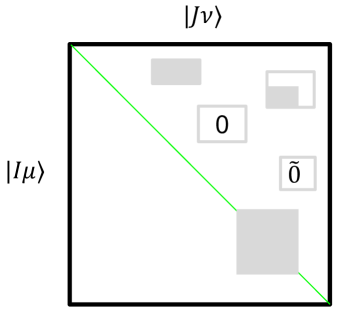
Figure 4: Schematic illustration of the structure of the symmetric Hamiltonian matrix $[H^{IJ}_{\mu\nu}]$

4.5 Selection of oCFGs and CSFs

The aim of selection is to find, iteratively, a better variational CSF space $P^{(k+1)}$ for the expansion of the wave function $|\Psi^{(k+1)}\rangle$ by feeding in the wave function $|\Psi^{(k)}\rangle=\sum_{|I\mu\rangle\in P^{(k)}}C^{I(k)}_{\mu}|I\mu\rangle$ of the previous iteration $k$. The selection of important CSFs consists of two steps, ranking and pruning. In the ranking step, proper rank values $\{A^{I}_{\mu}\}$ for the CSFs $\{|I\mu\rangle\}$ outside of $P^{(k)}$ will be evaluated. Those CSFs with rank values larger than the ranking-threshold $C_{\mathrm{q}}$ are then used to extend $P^{(k)}$ to $\bar{P}^{(k+1)}$. After constructing and diagonalizing the Hamiltonian matrix in $\bar{P}^{(k+1)}$, one obtains an improved wave function $|\bar{\Psi}^{(k+1)}\rangle=\sum_{|I\mu\rangle\in\bar{P}^{(k+1)}}\bar{C}^{I(k+1)}_{\mu}|I\mu\rangle$ with energy $\bar{E}^{(k+1)}$. In the pruning step, those CSFs in $\bar{P}^{(k+1)}$ but with coefficients smaller in absolute value than the pruning-threshold $C_{\mathrm{min}}$ are discarded, so as to reduce $\bar{P}^{(k+1)}$ to $P^{(k+1)}$. In principle, the Hamiltonian matrix in the reduced space $P^{(k+1)}$ should be reconstructed and diagonalized to obtain $|\Psi^{(k+1)}\rangle=\sum_{|I\mu\rangle\in P^{(k+1)}}C^{I(k+1)}_{\mu}|I\mu\rangle$ with energy $E^{(k+1)}$. However, this is not necessary for a sufficiently small $C_{\mathrm{min}}$: $\{C^{I(k+1)}_{\mu}\}$ and $E^{(k+1)}$ can simply be set to the corresponding $\{\bar{C}^{I(k+1)}_{\mu}\}$ and $\bar{E}^{(k+1)}$, respectively.

As for the ranking, an obvious choice⁹ is the (pruned²⁸) first-order coefficient in absolute value,

$$A^{I}_{\mu}(\mathrm{ASCI})=\left|\frac{\langle I\mu|H|\Psi^{(k)}\rangle}{E^{(k)}-H_{\mu\mu}^{II}}\right|=\left|\frac{\sum_{|J\nu\rangle\in P^{(k)}}H^{IJ}_{\mu\nu}C^{J(k)}_{\nu}}{E^{(k)}-H_{\mu\mu}^{II}}\right|\geq C_{\mathrm{q}}.$$ (62)

Albeit robust, Eq. (62) is computationally too expensive (due to the summation in the numerator) for the purpose of ranking. It was therefore simplified to

$$A^{I}_{\mu}(\mathrm{HCI})=\max_{|J\nu\rangle\in P^{(k)}}|H^{IJ}_{\mu\nu}C^{J(k)}_{\nu}|\stackrel{{\scriptstyle\mathrm{CSF}\rightarrow\mathrm{Det}}}{{\longrightarrow}}\max_{\nu\in P^{(k)}}|H_{\mu\nu}C_{\nu}^{(k)}|\geq\epsilon_{\mathrm{q}}$$ (63)

in the heat-bath CI approach (HCI)²⁵, which works with determinants though. Since the Hamiltonian matrix elements $H_{\mu\nu}$ over doubly connected determinants $|\Phi_{\mu}\rangle$ and $|\Phi_{\nu}\rangle$ depend only on the two-electron integrals (the absolute values of which can be sorted in descendent order and stored in memory from the outset), the ranking can be made extremely efficient: Those determinants $\{|\Phi_{\mu}\rangle\}$ that are doubly excited from $|\Phi_{\nu}\rangle\in P^{(k)}$ are never accessed if $|H_{\mu\nu}|<\epsilon_{\mathrm{q}}/|C_{\nu}^{(k)}|$⁸⁶. However, those determinants of high energies may become unimportant even though they satisfy condition (63). Therefore, the variational space determined by the integral-driven selection (63) is usually larger than that determined by the coefficient-driven selection (62), particularly when large basis sets are used (NB: this problem can partly be resolved by introducing an approximate denominator to condition (63), see the Supporting Information of Ref.⁸⁷). The recent development³⁰ of the adaptive sampling CI (ASCI) approach²⁸ reveals that sorting based algorithms can render the evaluation of $A_{\mu}^{I}$ (62) very fast. Here, the integral- and coefficient-driven algorithms are combined for the selection of doubly excited CSFs, viz.,

$$A^{I}_{\mu}(\mathrm{iCI})=\left|\frac{\sum_{J\in P^{(k)}}^{(\varepsilon_{k})}(\sum_{\nu,|J\nu\rangle\in P^{(k)}}H^{IJ}_{\mu\nu}C^{J(k)}_{\nu})}{E^{(k)}-H_{\mu\mu}^{II}}\right|\geq C_{\mathrm{q}},$$ (64)

where the summation over oCFG $J\in P^{(k)}$ is subject to the following condition

$$\max_{\nu}|\tilde{H}^{IJ}C_{\nu}^{J(k)}|\geq\varepsilon_{k}=\frac{1}{2}\varepsilon_{k-1},\quad J\in P^{(k)}.$$ (65)

Here, $\tilde{H}^{IJ}$ are the estimated upper bounds for the two-body Hamiltonian matrix elements $\langle I\mu|H_{2}^{2}|J\nu\rangle$ (see Table 1). Specifically, like condition (63), those oCFGs $\{I\}$ that are doubly excited from oCFG $J$ in $P^{(k)}$ are never accessed if $\tilde{H}^{IJ}<\varepsilon_{k}/\max_{\nu}|C_{\nu}^{J(k)}|$ (see Fig. 5). After this integral-driven screening, the individual CSFs $\{|I\mu\rangle\}$ of the selected oCFGs $\{I\}$ are further selected using their (approximate) first-order coefficients (64) (NB: the approximation arises from the restriction (65) on the summation over $J$ in the numerator), just like condition (62). Moreover, as indicated by the relation $\varepsilon_{k}=\frac{1}{2}\varepsilon_{k-1}$, the integral-threshold $\varepsilon_{k}$ is to be reduced by a factor of two with each iteration, meaning that the external oCFG space $Q$ is accessed incrementally (i.e., $Q(\varepsilon_{k})$). Since the calculation of $A^{I}_{\mu}(\mathrm{iCI})$ (64) becomes increasingly more expensive as the integral-threshold $\varepsilon_{k}$ gets reduced, we decide to repeat the selections for a given integral-threshold $\varepsilon_{k}$ until the following condition is fulfilled

$$S=\frac{|P^{(k)}_{j}\cap P^{(k)}_{j-1}|}{|P^{(k)}_{j}\cup P^{(k)}_{j-1}|}>S_{\mathrm{p}},$$ (66)

where the numerator (denominator) is the number of CSFs in the intersection (union) of the $P^{(k)}_{j}(\epsilon_{k})$ and $P^{(k)}_{j-1}(\epsilon_{k})$ spaces between two adjacent micro-iterations (designated by subscript $j$). Upon convergence at $j=t$, the space $P^{(k)}_{t}(\epsilon_{k})$ is diagonalized via the iVI approach^{80, 81} to obtain $|\Psi^{(k+1)}\rangle$ and $E^{(k+1)}$. Before going to the next macro-iteration, Algorithm 4 is invoked to decide whether the rotation of orbitals and update of $\epsilon_{k}$ need to be performed. The algorithm also decides when to terminate the selection.

1 if Orbital rotation is allowed then

2       if $|E^{(k+1)}-E^{(k)}|\leq 10\Delta_{\mathrm{e}}$ then

3             Construct and diagonalize the one-particle reduced density matrix to generate natural orbitals (NO) $\{\phi_{p}^{(k+1)}\}$, followed by integral transformation and rediagonalization of $P^{(k)}_{t}(\varepsilon_{k})$.

4             if $\{\phi_{p}^{(k+1)}\}$ are converged then

5                  $\varepsilon_{k+1}=\varepsilon_{k}/2$ and switch off orbital rotation.

6            else

7                  $\varepsilon_{k+1}=\varepsilon_{k}$.

8             end if

9            

10      else

11             $\varepsilon_{k+1}=\varepsilon_{k}/2$.

12       end if

13      return No.

14else

15       if $|E^{(k+1)}-E^{(k)}|\leq\Delta_{\mathrm{e}}$ then

16             return Yes;

17      else

18             $\varepsilon_{k+1}=\varepsilon_{k}/2$ , return No.

19       end if

20      

21 end if

22

Algorithm 4 Determination of rotation of orbitals and update of $\varepsilon_{k}$. Return Yes to terminate the selection or No to go next iteration. The condition for the convergence of NOs is as follows. The NOs $\{\phi_{p}^{(k+1)}\}$ and $\{\phi_{p}^{(k)}\}$ are related by $\phi_{p}^{(k+1)}=\sum_{q}c_{qp}\phi_{q}^{(k)}$. If $\exists q\text{ s.t. }|C_{qp}|\geq 0.99$, $\phi_{p}^{(k+1)}$ is considered to be converged (the same as $\phi_{q}^{(k)}$). If the sum of the occupation numbers of the converged NOs deviates from the total number of correlated electrons by less than 0.05, $\{\phi_{p}^{(k+1)}\}$ are considered to be the same as $\{\phi_{p}^{(k)}\}$.

To illustrate the above algorithm more clearly, a flowchart is provided in Fig. 6. Simply put, given an integral-threshold $\varepsilon$ to confine the accessible external oCFG space $Q(\varepsilon)$ (macro-iteration), the variational CSF space $P(\varepsilon)$ is updated iteratively until convergence (micro-iteration). Repeat this with a reduced $\varepsilon$ until no new NOs are needed. As for the thresholds, the dynamically adjusted integral-threshold $\varepsilon$ affects only the number of iterations; both $S_{\mathrm{p}}$ and $\Delta_{\mathrm{e}}$ can be set to conservative values (e.g., 0.95 and $3\times 10^{-4}$, respectively); the ranking-threshold $C_{\mathrm{q}}$ can simply be chosen to be the same as the coefficient pruning-threshold $C_{\mathrm{min}}$. Therefore, only $C_{\mathrm{min}}$ is truly a free parameter, which controls the size of the variational space and hence the final accuracy. It also deserves to be mentioned that the integral-threshold $\epsilon$ is usually larger than $C_{\mathrm{min}}/10$ upon termination of the selection.

The above algorithm is truly efficient. However, there may exist a memory bottleneck even if the external space is accessed only incrementally. This bottleneck can be resolved by decomposing the external space into disjoint subsets $\{Q_{s}\}$ (see Sec. 5), such that only one subspace is accessed at a time, with no communications between different subspaces. This leads to a modified algorithm shown in Fig. 7. The major difference from the previous algorithm lies in that the oCFGs $\{I\}\in Q_{s}$ have to be selected individually according to condition (65). That is, a doubly excited oCFG is first generated but is then dumped if it does not fulfill condition (65).

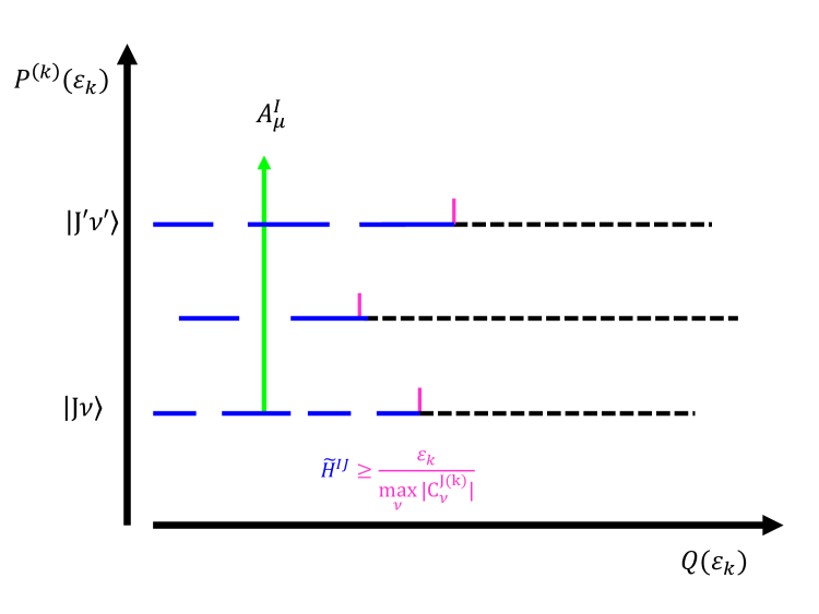
Figure 5: Illustration of the iCI ranking (64): At each macro-iteration $k$, doubly excited oCFGs $\{I\}$ from an oCFG $J\in P^{(k)}$ are retained only if they satisfy $\tilde{H}^{IJ}\geq\varepsilon_{k}/\max_{\nu}|C_{\nu}^{J(k)}|$ (broken blue lines); those unimportant oCFGs are not accessed at all (dash black lines); some oCFGs of $P^{(k)}$ do not contribute to $A_{\mu}^{I}$ due to the restriction (65) (blanks between blue lines).

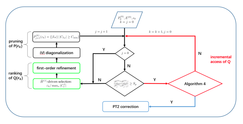
Figure 6: Flowchart for iCI selection (Scheme I)

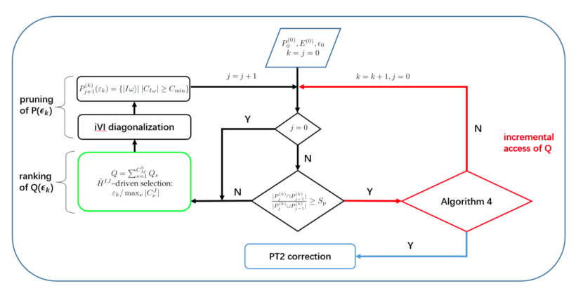
Figure 7: Flowchart for iCI selection (Scheme II)

5 Constraint-based Epstein-Nesbet PT2

Having determined a high-quality yet compact variational CSF space $P$ and hence the zeroth-order eigenpairs $\{E_{i}^{(0)},|\Psi_{i}^{(0)}\rangle\}$, we are now ready to account for the dynamic correlation via, e.g., the state-specific Epstein-Nesbet second-order perturbation theory (PT2)^{78, 79}

$$E_{c,i}^{(2)}=\sum_{|I\mu\rangle\in Q}\frac{\left|\langle I\mu|H|\Psi_{i}^{(0)}\rangle\right|^{2}}{E_{i}^{(0)}-H_{\mu\mu}^{II}}=\sum_{|I\mu\rangle\in Q}\frac{\left|\sum_{|J\nu\rangle\in P}H^{IJ}_{\mu\nu}C^{J}_{\nu,i}\right|^{2}}{E_{i}^{(0)}-H_{\mu\mu}^{II}}.$$ (67)

One problem associated with expression (67) lies in that it is memory intensive: The number of external CSFs $\{|I\mu\rangle\}$ scales as $N_{\mathrm{csf}}n_{o}^{2}n_{v}^{2}$, with $N_{\mathrm{csf}}$ being the number of CSFs $\{|J\nu\rangle\}$ in $P$. To reduce the memory requirement, we adopt the constraint PT2 algorithm proposed recently by Tubman et al.³¹. The basic idea is to decompose the external space $Q$ into disjoint subsets $\{Q_{s}\}$. For instance, the triplet constraints give rise to $C_{N_{\mathrm{orb}}}^{3}$ subsets, each of which is characterized by a particular set of three numbers $(p,q,r)$ ($p>q>r$) that specify the three highest occupied spatial orbitals in the oCFGs. That is, all the orbitals are unoccupied in the oCFGs if they are higher than $r$ but different from $p$ and $q$, i.e., $(0,\cdots,0,n_{p},0,\cdots,0,n_{q},0,\cdots,0,n_{r})$ in which $n_{p},n_{q},n_{r}\in[1,2]$. Such subspaces can readily be generated by adding one and two electrons into the first- and second-order residues of the $P$ space, respectively, with the following rules: Given a triplet $(p,q,r)$ that defines, say, subspace $Q_{s}$, a valid first-order residue can have at most one zero, whereas a valid second-order residue can have at most two zeros in the occupation numbers $(m_{p},m_{q},m_{r})$. If present, they must be filled with at least one electron. If singly occupied, $p/q/r$ can still accept one electron. Except for these on-site cases, only those orbitals lower than $r$ can accept electrons (if any). More importantly, valid residues, whether first- or second-order, are located continuously in different segments of the sorted residue array OrbOccBinary. The number of such segments is at most $3\times 3\times 3-1=26$ $(m_{p},m_{q},m_{r}\in[0,2]\backslash m_{p}=m_{q}=m_{r}=0)$. The head and tail of every segment can readily be found by using the bisection method. For a first-order residue with electron-depletion orbital $j$ recorded in array OrbIndx, the orbital occupied by the added electron corresponds to $i$ in $E_{ij}$. Note that the case of $i=j$ is also allowed here, for CSF $|J\mu\rangle$ may also contribute to the perturbation to another CSF $|J\nu\rangle$ from the same oCFG $J$. For a second-order residue with electron-depletion orbitals $j$ and $l$ ($\geq j$) recorded in array OrbIndx, the two orbitals occupied by the added two electrons corresponds to $i$ and $k$ $(\geq i)$ in $e_{ij,kl}$, after eliminating the zero- and one-body excitations [i.e., $\{i,k\}\cap\{j,l\}\neq\emptyset$; cf. Eq. (19)]. If $i<j$ in $E_{ij}$ or $k<l$ in $e_{ij,kl}$, a bra-ket inversion should be invoked when calculating the BCCs in terms of the diagrams documented in Table 2.

Being disjoint, the subspaces $\{Q_{s}\}$ can be embarrassingly parallelized, viz.

$$E_{c,i}^{(2)} =\sum_{s=1}^{C_{N_{\mathrm{orb}}}^{3}}\sum_{|I\mu\rangle\in Q_{s}}\frac{\left|\langle I\mu|H|\Psi_{i}^{(0)}\rangle\right|^{2}}{E_{i}^{(0)}-H_{\mu\mu}^{II}}.$$ (68)

Obviously, the same technique can be applied to the evaluation of $A_{\mu}^{I}$ (62)/(64) as well.

Another problem associated with Eq. (67) and also with Eq. (68) lies in that some of the singly and doubly excited CSFs from space $P$ are already present in $P$ and it is very expensive to check this (which is not the case for the ranking (62)/(63)/(64), because the number of important CSFs to be added to space $P$ is not very many, such that the double check of duplications in $P$ is very cheap). This issue can be resolved³¹ by precomputing the PT2-like energy $\bar{E}_{c,i}^{(2)}$ for such singly and doubly excited CSFs spanning $\bar{P}\in P$, which is finally subtracted from the PT2 energy $\tilde{E}_{c,i}^{(2)}$ for all the singly and doubly excited CSFs spanning $\tilde{Q}=Q\cup\bar{P}$:

$$E_{c,i}^{(2)} =\tilde{E}_{c,i}^{(2)}-\bar{E}_{c,i}^{(2)},$$ (69)

$$\tilde{E}_{c,i}^{(2)} =\sum_{s=1}^{C_{N_{\mathrm{orb}}}^{3}}\sum_{|I\mu\rangle\in\tilde{Q}_{s}}\frac{\left|\sum_{|J\nu\rangle\in P,|J\nu\rangle\neq|I\mu\rangle}H_{\mu\nu}^{IJ}C_{\nu,i}^{J}\right|^{2}}{E_{i}^{(0)}-H_{\mu\mu}^{II}},\quad\tilde{Q}_{s}=Q_{s}\cup\bar{P},$$ (70)

$$\bar{E}_{c,i}^{(2)} =\sum_{|I\mu\rangle\in\bar{P}}\frac{\left|\langle I\mu|H|\Psi_{i}^{(0)}\rangle-C_{\mu,i}^{I}H^{II}_{\mu\mu}\right|^{2}}{E_{i}^{(0)}-H_{\mu\mu}^{II}}$$ (71)

$$=\sum_{|I\mu\rangle\in\bar{P}}(C_{\mu,i}^{I})^{2}(E_{i}^{(0)}-H^{II}_{\mu\mu}),$$ (72)

where use of the relation $\langle I\mu|H|\Psi_{i}^{(0)}\rangle=C_{\mu,i}^{I}E_{i}^{(0)}$ has been made when going from Eq. (71) to Eq. (72). The negative term in the numerator of Eq. (71) arises from the fact that the diagonal terms (zero-body excitations) have been excluded in Eq. (70). This particular arrangement³¹ simplifies the evaluation of $\bar{E}_{c,i}^{(2)}$ via Eq. (72). Finally, if wanted, Eq. (70) can be approximated as

$$\tilde{E}_{c,i}^{(2)}(\tau) =\sum_{s=1}^{C_{N_{\mathrm{orb}}}^{3}}\sum_{I\in\tilde{Q}_{s}}^{(\tau)}\left[\sum_{\mu,|I\mu\rangle\in\tilde{Q}_{k}}\frac{\left|\sum_{|J\nu\rangle\in P,|J\nu\rangle\neq|I\mu\rangle}H_{\mu\nu}^{IJ}C_{\nu,i}^{J}\right|^{2}}{E_{i}^{(0)}-H_{\mu\mu}^{II}}\right],$$ (73)

where the summation over doubly excited oCFGs $\{I\}$ is subject to the following condition

$$\max_{\nu}|\tilde{H}^{IJ}C_{\nu,i}^{J}|\geq\tau,$$ (74)

with $\tau$ being a very conservative threshold for truncating the first-order interacting space $Q=\sum^{\oplus}_{s}Q_{s}$. Note that this truncation does not affect those oCFGs $\{I\}$ belonging to space $\bar{P}\in P$, because $\tau$ is orders of magnitude smaller than $\varepsilon$ employed for the selection of $P$ (cf. (65)). Therefore, contamination of $\bar{P}$ to $E_{c,i}^{(2)}(\tau)=\tilde{E}_{c,i}^{(2)}(\tau)-\bar{E}_{c,i}^{(2)}$ will not arise. It is expected that the difference $E_{c,i}^{(2)}(\tau=0)-E_{c,i}^{(2)}(\tau)$ is only weakly dependent on the coefficient pruning-threshold $C_{\mathrm{min}}$, i.e., $E_{c,i}^{(2)}(C^{S}_{\mathrm{min}},\tau=0)-E_{c,i}^{(2)}(C^{S}_{\mathrm{min}},\tau)\simeq E_{c,i}^{(2)}(C^{L}_{\mathrm{min}},\tau=0)-E_{c,i}^{(2)}(C^{L}_{\mathrm{min}},\tau)$ should hold for $C_{\mathrm{min}}^{S}<C_{\mathrm{min}}^{L}$. When this has been reached, we can get $E_{c,i}^{(2)}(C^{S}_{\mathrm{min}},\tau=0)$ from $E_{c,i}^{(2)}(C^{L}_{\mathrm{min}},\tau=0)+\left[E_{c,i}^{(2)}(C^{S}_{\mathrm{min}},\tau)-E_{c,i}^{(2)}(C^{L}_{\mathrm{min}},\tau)\right]$, so as to reduce the computational costs.

6 Pilot applications

6.1 C2

The proposed iCIPT2 approach is first applied to carbon dimer, a system that is known to have strong multireference characters even at the equilibrium distance. The calculations start with HF orbitals but which are rotated to natural orbitals (NO) during the selection procedure (see Algorithm 4). Although $D_{2h}$ instead of $D_{\infty h}$ symmetry is used, the terms of the states can be assigned correctly by considering simultaneously the degeneracy of the calculated energies and the correspondences between the $D_{2h}$ and $D_{\infty h}$ irreducible representations.

To compare directly with previous results, we first report the frozen-core ground state energies of C2 calculated at the equilibrium distance (1.24253 Å) with the cc-pVXZ (X = D, T, Q, 5) basis sets⁸⁸. It is seen from Table 5 and more clearly from Figs. 9 to 11 that the iCIPT2 energies converge steadily as the coefficient pruning-threshold $C_{\mathrm{min}}$ decreases, and become full agreement (within $0.1$ $\mathrm{mE_{h}}$) with the corresponding DMRG⁸⁹, ASCIPT2³¹ and HCIPT2^{90, 27} results when $C_{\mathrm{min}}=10^{-4}$, $10^{-4}$, $0.3\times 10^{-4}$ and $0.25\times 10^{-4}$ are used for the DZ, TZ, QZ and 5Z bases, respectively. Since the convergence is so smooth, one can stop at any desired accuracy. Encouraged by this, we further report the iCIPT2 excitation energies for the 8 lowest excited states of C2 at their equilibrium distances, which are known experimentally⁹¹. It is seen from Table 6 that the maximum and mean absolute deviations from the experimental values⁹¹ are only 0.02 eV and 0.01 eV, respectively, by the all-electron calculations with both the QZ and 5Z bases. The frozen-core approximation introduces noticeable errors (ca. 0.02 eV on average). Another issue related to all selection-based schemes lies in whether a smooth potential energy surface can be produced. This is indeed the case for iCIPT2. As can be seen from Fig. 8 (and Supporting Information), the all-electron FCI/DZ potential energy curve⁹² for the ground state of C2 is nicely reproduced by iCIPT2/DZ with $C_{\mathrm{min}}=10^{-4}$: the deviation of iCIPT2 from FCI is not larger than 0.1 $\mathrm{mE_{h}}$ for the whole range of the FCI curve and the crossing between ${}^{1}\Sigma_{g}^{+}$ and ${}^{1}\Delta_{g}$ at 3.10 bohrs is also reproduced. For comparison, the matrix product state-based linearized coupled-cluster (MPS-LCC) method⁹² deviates from FCI by 0.1–4.8 $\mathrm{mE_{h}}$ and exhibits a discontinuity at 3.10 bohrs. It also deserves to be mentioned that the iCIPT2 energy difference between the noninteracting C$\cdots$C and two carbon atoms is at most 1 $\mathrm{mE_{h}}$ for all the bases considered here, manifesting that iCIPT2 is nearly size consistent.

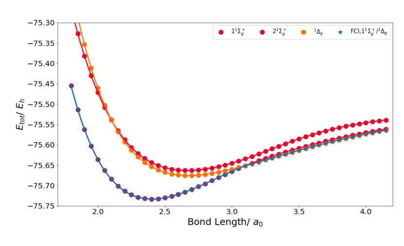
Figure 8: Potential energy curves for the lowest three states of C2 by all-electron iCIPT2/cc-pVDZ ($C_{\text{min}}=10^{-4}$). The all-electron FCI/cc-pVDZ results are taken from Ref.⁹².

Table 5: Frozen-core iCIPT2/cc-pVXZ (X = D, T, Q, 5) calculations of the ground state of C2 at $R=1.24253$ Å. $C_{\mathrm{min}}$: threshold for pruning configuration state functions (CSF) in the variational (var) space; $N_{\mathrm{cfg}}$: number of orbital configurations in the variational space; $N_{\mathrm{csf}}$: number of CSFs corresponding to $N_{\mathrm{cfg}}$; PT2: state-specific Epstein-Nesbet second-order perturbation theory.

						energy ($\mathrm{E_{h}}$)		wall time (second)
basis	$\text{C}_{\text{min}}/10^{-4}$	$N_{\text{cfg}}$	$N_{\text{csf}}$	$\tilde{N}_{\text{csf}}$a	$\tilde{N}_{\text{det}}$b	var	total	var	PT2	total
DZ	3.0	4025	11771	6662	22046	-75.725235	-75.728478	2.0	0.4	2.4
	1.0	10858	36043	20009	36043	-75.727359	-75.728514	5.8	0.9	6.7
	0.7	14840	51247	28405	101193	-75.727736	-75.728518	9.3	1.2	10.5
	0.5	19850	71054	39323	142051	-75.727989	-75.728520	13.4	1.6	15.0
	0.3	30023	113084	62566	230920	-75.728232	-75.728521	23.3	2.2	25.5
	DMRGd						-75.728556
	ASCIPT2e				300000	-75.72836	-75.72855
	HCIPT2f				28566	-75.7217	-75.7286(2)
TZ	3.0	7619	21222	11407	36670	-75.776765	-75.785171	9	3	12
	1.0	23951	77471	39342	135058	-75.781493	-75.785087	25	9	34
	0.7	34708	117741	59187	207007	-75.782402	-75.785071	39	13	52
	0.5	46186	162497	82205	292205	-75.782952	-75.785063	54	17	71
	0.3	78289	291552	145729	529906	-75.783710	-78.785045	104	29	133
	0.25	94256	358507	178041	652141	-75.783912	-75.785041	129	33	162
	0.2	117839	459603	227080	839058	-75.784120	-75.785036	171	42	213
	0.0c						-75.785022(3)
	DMRGd						-75.785054
	ASCIPT2e				300000	-75.78196	-75.78515
	HCIPT2f				28566	-75.7738	-75.7846(3)
QZ	3.0	9131	24350	13147	41483	-75.790913	-75.803425	51	14	65
	1.0	29750	91695	46530	156565	-75.797365	-75.802968	77	41	118
	0.7	44534	144199	71648	245693	-75.798640	-75.802882	110	60	170
	0.5	64498	218116	106986	373386	-75.799585	-75.802824	169	85	254
	0.3	112453	405609	194548	695920	-75.800617	-75.802760	338	147	485
	0.25	136467	503417	239787	864600	-75.800903	-75.802743	416	171	587
	0.2	164647	615634	295452	1073145	-75.801133	-75.802730	484	209	693
	0.0c						-75.802620(13)
	DMRGd						-75.802671
	ASCIPT2e				300000	-75.79807	-75.80290
	HCIPT2g						-75.80264
5Z	3.0	9512	25145	13563	42624	-75.793434	-75.809434	273	46	319
	1.0	33806	101439	51317	170618	-75.801447	-75.808479	396	132	528
	0.7	49422	154744	77314	261569	-75.802895	-75.808318	452	189	641
	0.5	71918	235234	115843	399168	-75.804043	-75.808190	590	275	865
	0.3	126783	442037	212308	749953	-75.805291	-75.808055	940	467	1407
	0.25	154888	551770	262589	934869	-75.805629	-75.808019	1032	595	1627
	0.2	197617	721564	340880	1225120	-75.805987	-75.807985	1305	726	2031
	0.0c						-75.807764(18)
	HCIPT2g						-75.80790(3)

• Number of CSFs after selection, among which about 0.5% have coefficients slightly smaller in absolute values than $C_{\mathrm{min}}$ (which is due to a final diagonalization).

• Estimated number of determinants according to the expression $\sum_{I}\frac{\tilde{N}_{\mathrm{csf}}^{I}}{N_{\mathrm{csf}}^{I}}N_{\mathrm{det}}^{I}$, with $N_{\mathrm{det}}^{I}$, $N_{\mathrm{csf}}^{I}$ and $\tilde{N}_{\mathrm{csf}}^{I}$ being the numbers of determinants, CSFs and selected CSFs of oCFG $I$, respectively.

• Extrapolated value by linear fit of the $E_{\mathrm{total}}$ vs. $|E_{c}^{(2)}|$ plot.

• Ref.⁸⁹.

• Ref.³¹.

• Ref.⁹⁰.

• Ref.²⁷.

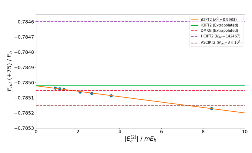
Figure 9: Comparison of the frozen-core ground state energies of C2 at $R=1.24253$ Å by different methods with cc-pVTZ. Blue dots refer to different $C_{\mathrm{min}}$ values in iCIPT2. The extrapolated values are -75.785022(3), -75.785054, -75.78515 and -75.7846(3) $\mathrm{E_{h}}$ for iCIPT2, DMRG⁸⁹, ASCIPT2³¹ and HCIPT2⁹⁰, respectively.

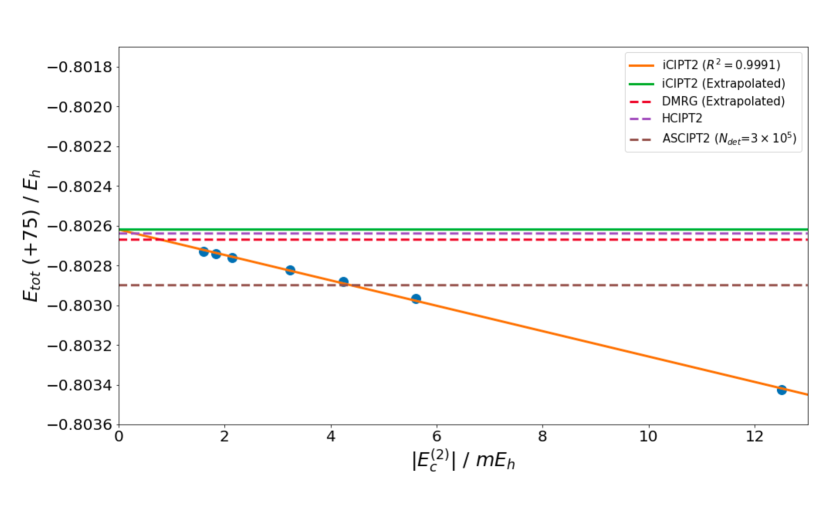
Figure 10: Comparison of the frozen-core ground state energies of C2 at $R=1.24253$ Å by different methods with cc-pVQZ. Blue dots refer to different $C_{\mathrm{min}}$ values in iCIPT2. The extrapolated values are -75.802620(13), -75.802671, -75.80264 and -75.80290 $\mathrm{E_{h}}$ for iCIPT2, DMRG⁸⁹, ASCIPT2³¹ and HCIPT2²⁷, respectively.

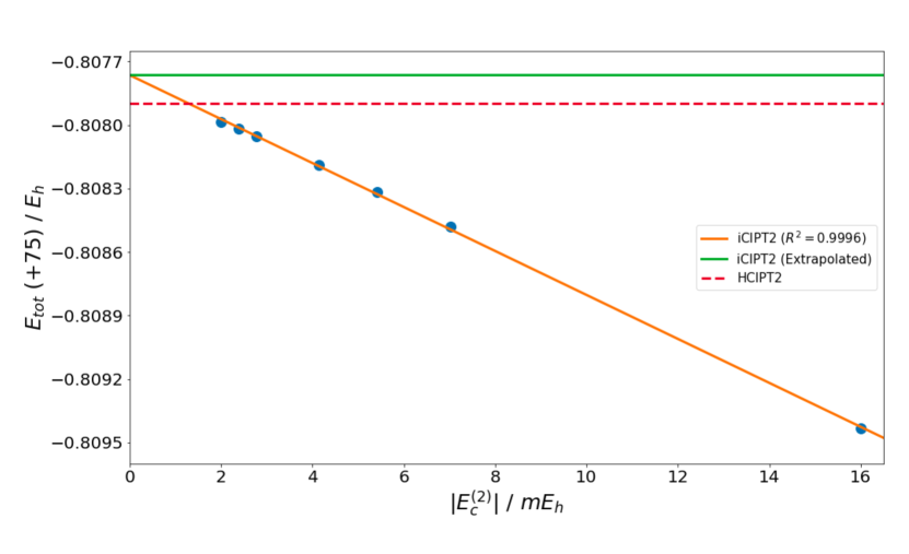
Figure 11: Comparison of the frozen-core ground state energies of C2 at $R=1.24253$ Å by different methods with cc-pV5Z. Blue dots refer to different $C_{\mathrm{min}}$ values in iCIPT2. The extrapolated values are -75.807764(18) and -75.80790(3) a.u. for iCIPT2 and HCIPT2²⁷, respectively.

Table 6: iCIPT2 adiabatic excitation energies of C2 with $C_{\mathrm{min}}$ being $0.3\times 10^{-4}$ and $0.5\times 10^{-4}$ for cc-pVQZ and cc-pV5Z, respectively. FZ: frozen-core; AE: all-electron; MAX: maximum absolute error; MAE: mean absolute error.

		adiabatic excitation energy (eV)
state	$R_{\text{eq}}$ (Å)a	$\Delta E_{\text{FC,QZ}}$	$\Delta E_{\text{AE,QZ}}$	$\Delta E_{\text{FC,5Z}}$	$\Delta E_{\text{AE,5Z}}$	$\Delta E_{\text{FC,5Z}}$b	Experimenta
$X^{1}\Sigma_{g}^{+}$	1.24253	0.00	0.00	0.00	0.00	0.00	0.00
$a^{3}\Pi_{u}$	1.312	0.07	0.09	0.07	0.09	0.07	0.09
$b^{3}\Sigma_{g}^{-}$	1.369	0.77	0.81	0.77	0.81	0.78	0.80
$A^{1}\Pi_{u}$	1.318	1.03	1.05	1.03	1.05	1.03	1.04
$c^{3}\Sigma_{u}^{+}$	1.208	1.17	1.14	1.16	1.12	1.16	1.13
$B^{1}\Delta_{g}$	1.385	1.48	1.52	1.48	1.52	1.49	1.50
$B^{\prime 1}\Sigma_{g}^{+}$	1.377	1.89	1.93	1.90	1.93	1.90	1.91
$d^{3}\Pi_{g}$	1.266	2.51	2.49	2.50	2.47	2.50	2.48
$C^{1}\Pi_{g}$	1.255	4.30	4.27	4.28	4.25	4.29	4.25
MAX		0.05	0.02	0.03	0.02	0.04
MAE		0.03	0.01	0.02	0.01	0.02

• Ref.⁹¹.

• HCIPT2²⁷.

6.2 O2

One particularly good feature of the CSF-based iCIPT2 lies in that it can describe the ground and excited states of arbitrary open-shell systems. To show this, we calculate the potential energy curves of the lowest three states (i.e., ${}^{3}\Sigma_{g}^{-}$, ${}^{1}\Delta_{g}$ and ${}^{1}\Sigma_{g}^{+}$) of O2, which are most relevant to chemical, biological and photocatalytic reactions. The potential energy curves (see Fig. 12) are obtained by cubic spline interpolations of the pointwise energies (cf. Supporting Information) calculated by iCIPT2/cc-pVQZ with $C_{\text{min}}=0.5\times 10^{-4}$. It can be seen from the inset of Fig. 12 that the ${}^{3}\Sigma_{g}^{-}$ state is crossed by ${}^{1}\Delta_{g}$ and ${}^{1}\Sigma_{g}^{+}$ around 2.07 and 2.21 Å, respectively. Some spectroscopic constants of O2 are presented in Table 7. The equilibrium bond length, harmonic vibrational frequency and dissociation energy (after correcting for zero-point energy) of the ground state ${}^{3}\Sigma_{g}^{-}$ are 1.2085 Å, 1573.9 cm^-1 and 5.0936 eV, respectively, which are very close to the corresponding experimental values (1.2075 Å, 1580 cm^-1 and 5.080 eV)⁹³. The adiabatic excitation energies of ${}^{1}\Delta_{g}$ and ${}^{1}\Sigma_{g}^{+}$ are 0.93 and 1.59 eV, respectively, which are again very close to the corresponding experimental values (0.95 and 1.61 eV)⁹⁴.

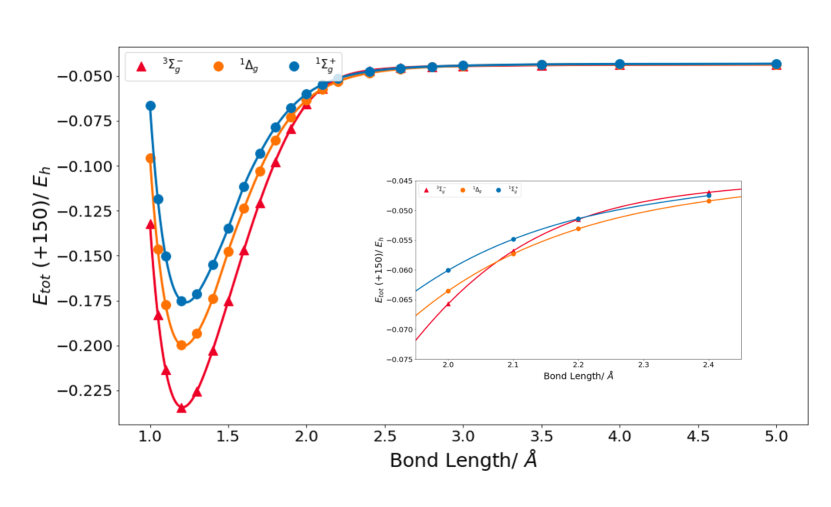
Figure 12: Potential energy curves of the ${}^{3}\Sigma_{g}^{-}$, ${}^{1}\Delta_{g}$ and ${}^{1}\Sigma_{g}^{+}$ states of oxygen by iCIPT2/cc-pVQZ.

Table 7: Spectroscopic constants of the ${}^{3}\Sigma_{g}^{-}$, ${}^{1}\Delta_{g}$ and ${}^{1}\Sigma_{g}^{+}$ states of O2. $\omega_{e}$: harmonic vibrational frequency; ZPE: zero-point energy; $D_{e}$: dissociation energy after correcting ZPE; $\Delta E_{\mathrm{v}}$/$\Delta E_{\mathrm{a}}$: vertical/adiabatic excitation energy.

state	$R_{e}/$Å	$\omega_{e}/\mathrm{cm^{-1}}$	$\omega_{e}X_{e}/\mathrm{cm^{-1}}$	$\omega_{e}Y_{e}/\mathrm{cm^{-1}}$	$\omega_{e}Z_{e}/\mathrm{cm^{-1}}$	ZPE/eV	$D_{e}$/eV	$\Delta E_{\mathrm{v}}$/eV	$\Delta E_{\mathrm{a}}$/eV
${}^{3}\Sigma_{g}^{-}$	1.2085	1573.9	15.866	3.0327	0.4847	0.0976	5.0936	0.00	0.00
${}^{1}\Delta_{g}$	1.2164	1503.3	21.256	1.4019	-0.0609	0.0932	4.1616	0.93	0.93
${}^{1}\Sigma_{g}^{+}$	1.2291	1429.4	19.870	2.5417	0.3715	0.0886	3.5054	1.60	1.59

6.3 Cr2

Compared with C2 and O2, Cr2 is a more stringent test system for quantum chemical methods due to strong entanglement between the static and dynamic components of correlation. The frozen-core (24e, 30o) and all-electron (48e, 42o) FCI spaces consist of $1.17\times 10^{14}$ ($9.35\times 10^{14}$) and $1.42\times 10^{21}$ ($1.56\times 10^{22}$) CSFs (determinants), respectively. In order to compare directly with the previous results^{95, 89, 28, 87}, the ground state energy of Cr2 at an interatomic distance of 1.5 Å  is calculated with the Ahlrichs SV basis⁹⁶. Noticing that the calculated energy may be dependent on how the core orbitals are defined, both the Hartree-Fock and CAS(12e, 12o) cores are considered in the frozen-core calculations. The remaining orbitals are natural orbitals that are optimized during the selection procedure (see again Algorithm 4). The results are presented in Table 8. For a better illustration, the results by the Hartree-Fock core and all-electron calculations are further plotted in Figs. 13 and 14, respectively. Apart from the excellent agreement between the extrapolated values by all the methods quoted here, only the following points need to be pointed out: (1) The all-electron iCIPT2 calculations with $C_{\mathrm{min}}$ smaller than $0.3\times 10^{-4}$ cannot be performed due to shortage of memory space. Nevertheless, the calculated data is enough for a high quality linear fit ($R^{2}=0.9996$), yielding an extrapolated energy (-2086.44474 $\mathrm{E_{h}}$) that almost coincides with the extrapolated DMRG (-2086.44478 $\mathrm{E_{h}}$)⁸⁹ and HBCIPT2 (-2086.44475 $\mathrm{E_{h}}$)⁸⁷ values; (2) It is a bit surprising that the all-electron DMRG (m = 8000) energy matches the iCIPT2 one with $C_{\mathrm{min}}$ around $1.5\times 10^{-4}$, instead of some value below $0.2\times 10^{-4}$ (cf. the Hartree-Fock core calculations); (3) Although the wall times are reported here, they cannot be compared with those by the closely related ASCIPT2³⁰ and HBCIPT⁸⁷ methods, simply because the parallel calculations were performed with different numbers of CPU cores of different computers.

We further analyze the variational wave functions. As can be seen from Tables 9 and 10, the highest excitation rank (relative to the leading, closed-shell oCFG) and the highest seniority number of the oCFGs in the variational space amount to 10 and 12, respectively, in the frozen-core calculations. It can also be seen from Fig. 15 that essentially all the NOs are sampled by the selection procedure. Although not documented here, the same hold also for the all-electron calculations. All these establish that Cr2 is beyond the capability of single-reference methods.

Table 8: iCIPT2/SV calculations of Cr₂ at $R=1.5$ Å. For additional explanations see Table 5.

					energy ($\mathrm{E_{h}}$)		wall time (sec)
$\text{C}_{\text{min}}/10^{-4}$	$N_{\text{cfg}}$	$N_{\text{csf}}$	$\tilde{N}_{\text{csf}}$	$\tilde{N}_{\text{det}}$	var	total	var	PT2	total
Hartree-Fock core, (24e, 30o)
3.0	19442	98889	32416	121239	-2086.391741	-2086.418993	66	16	82
2.0	31763	176002	56882	219688	-2086.398124	-2086.419391	99	28	127
1.0	72982	486500	143981	583862	-2086.406023	-2086.419964	243	65	308
0.7	109678	791934	227610	944209	-2086.408963	-2086.420184	312	100	412
0.5	164704	1282820	359831	1524930	-2086.411391	-2086.420369	534	171	705
0.3	299454	2629089	703541	3072786	-2086.414197	-2086.420576	961	496	1457
0.25	371511	3422901	892099	3935360	-2086.414997	-2086.420631	1236	723	1959
0.2	457771	4452704	1147403	5131066	-2086.415723	-2086.420683	1452	1026	2478
0.0a						-2086.421056(35)
DMRG (m=8000)b						-2086.420780
DMRG (m=$\infty$)b						-2086.420948
HCIPT2c						-2086.420934 (5)
HCIPT2d						-2086.42107
FCIQMCe						-2086.4212(3)
CAS(12e, 12o) core, (24e, 30)
3.0	19474	99466	32333	120826	-2086.392182	-2086.419290	52	16	68
2.0	31713	176201	56766	219417	-2086.398555	-2086.419751	77	28	105
1.0	72811	486435	143675	582778	-2086.406445	-2086.420352	170	67	237
0.7	112885	822216	232969	966906	-2086.409557	-2086.420565	293	109	402
0.5	163864	1276103	358252	1518671	-2086.411808	-2086.420755	435	175	610
0.3	298404	2618279	701672	3064718	-2086.414594	-2086.420960	868	504	1372
0.25	370538	3412674	890956	3930293	-2086.415389	-2086.421014	1122	746	1868
0.2	458347	4477991	1148115	5133858	-2086.416130	-2086.421076	1262	1020	2282
0.0a						-2086.421470(16)
HCIPT2c						-2086.421385(5)
HCIPT2d						-2086.42152
All-electron, (48e, 42o)
2.0	34765	187681	60650	232203	-2086.415171	-2086.442935	205	125	330
1.0	81270	522899	156280	628276	-2086.424817	-2086.443505	433	394	827
0.7	128132	900081	256897	1055972	-2086.428629	-2086.443755	761	662	1423
0.5	188398	1420214	399815	1679269	-2086.431489	-2086.443933	1871	1115	2663
0.3	349927	2972292	796412	3447559	-2086.435048	-2086.444149	2121	2309	4430
0.0a						-2086.444740(41)
DMRG (m=8000)b						-2086.443173
DMRG (m=$\infty$)b						-2086.44478(32)
HCIPT2c						-2086.444586(10)
HCIPT2d						-2086.44475
ASCIf						-2086.44325

• Extrapolated value by linear fit of the $E_{\mathrm{total}}$ vs. $|E_{c}^{(2)}|$ plot ($R^{2}>0.999$).

• Ref.⁸⁹.

• Ref.⁸⁷ (weighted quadratic fit).

• Ref.⁸⁷ (linear fit).

• Ref.⁹⁵.

• Ref.²⁸.

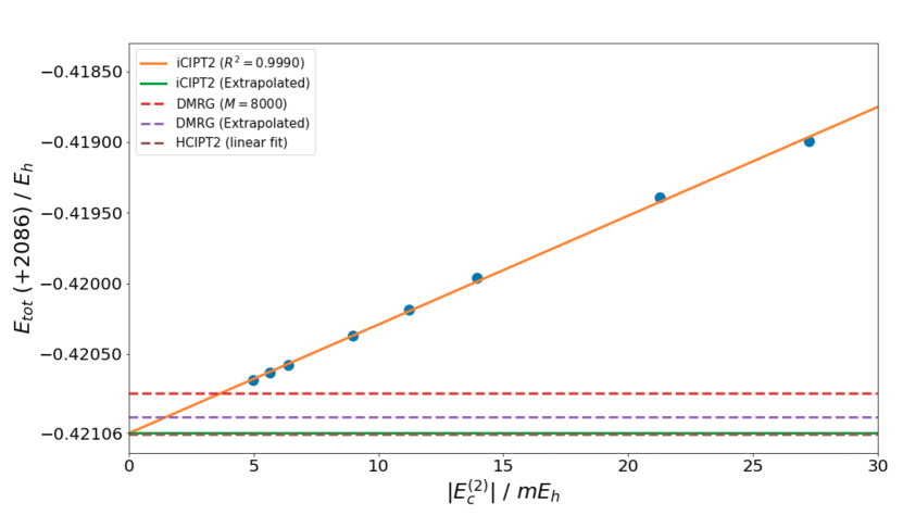
Figure 13: Comparison of the Hartree-Fock core ground state energies of Cr2 at $R=1.5$ Å by different methods with the Ahlrichs SV basis. Blue dots refer to different $C_{\mathrm{min}}$ values in iCIPT2. The extrapolated values are -2086.421056(35), -2086.420948, -2086.42107 $\mathrm{E_{h}}$ for iCIPT2, DMRG⁸⁹ and HCIPT2⁸⁷, respectively.

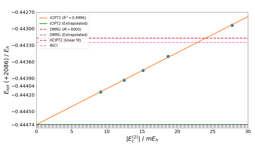
Figure 14: Comparison of the all-electron ground state energies of Cr2 at $R=1.5$ Å by different methods with the Ahlrichs SV basis. Blue dots refer to different $C_{\mathrm{min}}$ values in iCIPT2. The extrapolated values are -2086.444740(41), -2086.44478(32), -2086.44475 and -2086.44325 $\mathrm{E_{h}}$ for iCIPT2, DMRG⁸⁹, HCIPT2⁸⁷ and ASCI²⁸ respectively.

Table 9: Excitation ranks of oCFGs (relative to the leading, closed-shell oCFG) in the variational space ($C_{\text{min}}=0.2\times 10^{-4}$) for Cr2 at $R=1.5$ Å [Hartree Fock core, (24e, 30o)]. For additional explanations see Table 5.

Excitation rank	$N_{\text{cfg}}$	$\tilde{N}_{\text{csf}}$	Contribution
0	1	1	59.6262%	59.6262%
1	20	20	0.0720%	59.6982%
2	1663	2709	29.3529%	89.0511%
3	24218	52509	0.8260%	89.8771%
4	115938	291396	7.6426%	97.5197%
5	93636	236271	0.5409%	98.0606%
6	120545	307891	1.4567%	99.5173%
7	48520	128955	0.1965%	99.7138%
8	35856	87461	0.2197%	99.9335%
9	11539	28595	0.0407%	99.9742%
>=10	5835	11595	0.0258%	100.0000%

Table 10: Seniority numbers of oCFGs in the variational space ($C_{\text{min}}=0.2\times 10^{-4}$) for Cr2 at $R=1.5$ Å [Hartree Fock core, (24e, 30o)]. For additional explanations see Table 5.

Seniority	$N_{\text{cfg}}$	$N_{\text{csf}}$	$\tilde{N}_{\text{csf}}$	Contribution
0	10146	10146	10146	72.5872%	72.5872%
2	19669	19669	19669	1.1228%	73.7100%
4	131839	263678	190184	23.2162%	96.9262%
6	142933	714665	318859	0.9821%	97.9083%
8	123231	1725234	448527	2.0114%	99.9197%
10	24986	1049412	127341	0.0621%	99.9818%
12	4919	649308	32503	0.0182%	100.0000%
14	48	20592	174	0.0000%	100.0000%

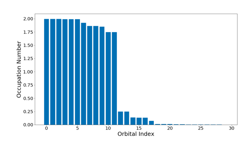
Figure 15: Occupation numbers of natural orbitals ($C_{\text{min}}=0.2\times 10^{-4}$) for Cr₂ at $R=1.5$ Å [Hartree Fock core, (24e, 30o)].

6.4 C6H6

As a final example, the frozen-core ground state energy of benzene at equilibrium⁹⁷ is calculated with iCIPT2/cc-pVDZ. Although benzene is not really a strongly correlated system, the (30e, 108o) space consists of $6.95\times 10^{33}$ CSFs or $9.5\times 10^{34}$ determinants and therefore represents a great challenge if one wants to obtain nearly FCI result. The calculations employ $D_{2h}$ symmetry. The results with HF and natural orbitals are presented in Table 11. A linear extrapolation of the calculated correlation energies is further plotted in Fig. 16. Several points deserve to be mentioned here:

1. The largest calculation (with $C_{\mathrm{min}}=5\times 10^{-5}$) involves $1.00\times 10^{6}$ ($1.38\times 10^{6}$) CSFs in the variational space and $8.69\times 10^{11}$ ($1.38\times 10^{12}$) CSFs in the first-order interacting space and took 1215.75 (2225.85) minutes of wall time on a single node with two 2.60 GHz Intel Xeon E5-2640 v3 processors, when HF (natural) orbitals are used. This gives rise to -822.4 (-833.3) $\mathrm{mE_{h}}$ for the overall correlation energy, which is 95.3% (96.8%) of the extrapolated value $-863.3$ (-861.1 $\mathrm{mE_{h}}$).

2. The extrapolated correlation energies using natural and HF orbitals differ by only 2.2 $\mathrm{mE_{h}}$, indicating that the present iCIPT2 calculations are essentially converged.

3. The atomization energies of benzene are 55.307 and 55.245 eV for the HF and natural orbital based calculations, respectively.

4. It is very much surprising that the majority of the CSFs in the variational space are open shells, e.g., $1.6\times 10^{4}$ closed-shell CSFs, $2.7\times 10^{4}$ CSFs with 2 unpaired electrons, $4.1\times 10^{5}$ CSFs with 4 unpaired electrons, $3.6\times 10^{5}$ CSFs with 6 unpaired electrons, and $5.7\times 10^{5}$ CSFs with 8 unpaired electrons in the case of $C_{\mathrm{min}}=5\times 10^{-5}$ with natural orbitals.

Table 11: Calculated correlation energies $E_{c}$ ($=E_{c}^{\mathrm{var}}+E_{c}^{(2)}$) for benzene at equilibrium (D_2h symmetry; cc-pVDZ; (30e, 108o); $E_{\mathrm{HF}}=-230.721819$ $\mathrm{E_{h}}$).

$C_{\text{min}}$	HF orbitals			Natural orbitals
	$E_{c}^{\mathrm{var}}/\mathrm{mE_{h}}$	$E_{c}/\mathrm{mE_{h}}$	$T$$/s$a	$E_{c}^{\mathrm{var}}/\mathrm{mE_{h}}$	$E_{c}/\mathrm{mE_{h}}$	$T$$/s$a
10.0	-589.336	-802.909	301	-612.591	-816.724	379
5.0	-649.922	-810.127	837	-656.729	-819.366	669
3.0	-667.714	-812.884	1309	-676.147	-822.384	1481
2.0	-675.959	-814.997	2363	-687.627	-824.699	2794
1.5	-681.083	-816.564	3036	-695.623	-826.403	5066
1.0	-688.358	-818.664	9875	-707.243	-828.807	15206
0.9	-690.363	-819.194	12712	-710.440	-829.460	22335
0.8	-692.695	-819.797	17447	-714.110	-830.223	38399
0.7	-695.422	-820.487	26334	-718.441	-831.135	49238
0.6	-698.767	-821.330	42053	-723.616	-832.289	77344
0.5	-703.066	-822.427	72945	-729.983	-833.690	133551
0.0		-863.32(54)b			-861.05(51)c

• (1) CPU: 2.60 GHz Intel Xeon E5-2640 v3$\times$2, 16 cores; (2) memory: 128 Gb; (3) parallelization: OpenMP, 16 threads.

• Extrapolated value by linear fit ($E_{c}=0.34257\times|E_{c}^{(2)}|-863.32$ with $R^{2}=0.99992$) of the $E_{\mathrm{c}}$ vs. $|E_{\mathrm{c}}-E_{\mathrm{c}}^{\mathrm{var}}|$ with $C_{\text{min}}=\{1.0,0.9,\cdots,0.6,0.5\}\times 10^{-4}$.

• Extrapolated value by linear fit ($E_{c}=0.26498\times|E_{c}^{(2)}|-861.05$ with $R^{2}=0.9997$) of the $E_{\mathrm{c}}$ vs. $|E_{\mathrm{c}}-E_{\mathrm{c}}^{\mathrm{var}}|$ with $C_{\text{min}}=\{3.0,2.0,\cdots,0.6,0.5\}\times 10^{-4}$.

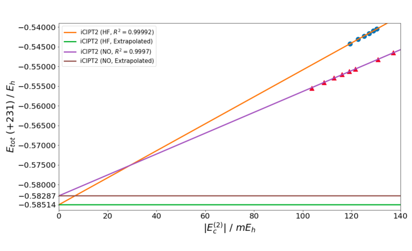
Figure 16: Extrapolation of the correlation energy of benzene.

7 Conclusions and outlook

A very efficient and robust approach, iCIPT2, has been developed for systems of strongly correlated electrons. It combines well-defined algorithms for the selection of important oCFGs/CSFs over the whole Hilbert space with a very efficient implementation of Epstein-Nesbet second-order perturbation theory. Effectively only one parameter, the coefficient pruning-threshold $C_{\mathrm{min}}$, is invoked to control the size of the variational space that has no CSFs with coefficients smaller in absolute value than $C_{\mathrm{min}}$. Another salient feature of iCIPT2 lies in that the external space is split into disjoint subsets, each of which is accessed only incrementally during the selection procedure. As has been demonstrated, iCIPT2 can describe very well not only the ground states but also the excited states of closed- and open-shell systems. In line with the previous findings²⁷, once the total-PT2 correlation energy plot has reached a linear domain, the extrapolated total correlation energy is very close to the FCI value. Nonetheless, one should be aware that, even in the linear regime, the slope of the total-PT2 correlation energy plot depends, albeit weakly, on what MRPT2 and what orbitals are used (cf. Fig. 16). Such dependence may result in an uncertainty of a few millihartrees. While such accuracy is sufficient for most applications, one may consider to go beyond MRPT2 by formulating, e.g., a size-consistent incomplete model space LCC^{98, 99, 100}.

Supporting Information

The Supporting Information is available free of charge, including the proof of inequality (56) as well as the pointwise energies of C2 and O2.

The research of this work was supported by NSFC (Grant Nos. 21033001 and 21973054) and the North Dakota University System.

Appendix A Data structure of the Hamiltonian matrix

A.1 Diagonal blocks

Both the first-order coefficient (64) and second-order energy (68) require the diagonal matrix elements $H^{II}_{\mu\mu}$ $(\mu\in[0,N_{S,S}^{I}-1])$, the evaluation of which is not cheap due to summations over both orbitals and orbital pairs. However, the calculation can be simplified by introducing a common reference oCFG with occupation numbers $\{\omega_{k}\}$ for the spatial orbitals. As shown by Eq. (46), apart from the first, constant term in the curly brackets, the remaining two terms therein depend only on the differential occupations $\{\Delta_{i}^{I}\}$, whereas both $i$ and $j$ in $\langle I\mu|e^{1}_{ij,ji}|I\mu\rangle$ are singly occupied. As discussed in Sec. 4.2, after introducing the reduced spatial orbital indices $\{\bar{i},\bar{j},\bar{k},\bar{l}\}$, oCFGs with the same number of singly occupied orbitals share the same BCCs $\langle I\mu|e^{1}_{\bar{i}\bar{j},\bar{j}\bar{i}}|I\mu\rangle$. Moreover, the off-diagonal elements $H^{II}_{\mu\nu}$ within a diagonal block also depend only on the BCCs $\langle I\mu|e^{1}_{\bar{i}\bar{j},\bar{j}\bar{i}}|I\nu\rangle$.

To store $\langle I\mu|e^{1}_{\bar{i}\bar{j},\bar{j}\bar{i}}|I\mu\rangle$, we define the compound index $(ij)=\frac{\bar{j}(\bar{j}-1)}{2}+\bar{i}$ and a matrix ${\color[rgb]{0,0,1}Ccf\_Dg}$ with elements ${\color[rgb]{0,0,1}Ccf\_Dg}[\mu][(ij)]=\langle I\mu|e^{1}_{\bar{i}\bar{j},\bar{j}\bar{i}}|I\mu\rangle$. The integrals in the summation $\sum_{i<j}(ij|ji)\langle I\mu|e^{1}_{\bar{i}\bar{j},\bar{j}\bar{i}}|I\mu\rangle$ are stored in an array ${\color[rgb]{0,0,1}Int}$ with elements ${\color[rgb]{0,0,1}Int}[(ij)]=(ij|ji)$. This way, the summation over $i$ and $j$ can be viewed as the inner product of vectors ${\color[rgb]{0,0,1}Ccf\_Dg}[\mu][*]$ and ${\color[rgb]{0,0,1}Int}[*]$. The calculation of all the diagonal elements within a diagonal block can then be viewed as the matrix-vector product of matrix ${\color[rgb]{0,0,1}Ccf\_Dg}[*][*]$ and vector ${\color[rgb]{0,0,1}Int}[*]$, as shown in Algorithm 5.

1 (Precalculation) Given the reference oCFG $\Omega$ with occupation numbers $\{\omega_{k}\}$, calculate $C=\frac{1}{2}\sum_{i}\omega_{i}[h_{ii}\varepsilon_{i}+(\omega_{i}-2)g_{ii}]$, $B_{i}=\varepsilon_{i}+(\omega_{i}-1)g_{ii}$ and $g_{ij}$, with $\varepsilon_{i}$ and $g_{ij}$ defined in Eqs. (44) and (45).

2Input oCFG $I$ and store nonzero differential occupations (relative to $\Omega$) in an array $\{(i,\Delta_{i}^{I})\}$.

3Calculate $C^{\prime}=C+\sum_{i}\Delta_{i}^{I}B_{i}+\sum_{i\leq j}\Delta_{i}^{I}g_{ij}\Delta_{j}^{I}$.

4Get molecular integrals ${\color[rgb]{0,0,1}Int}[(ij)]=(ij|ji)$

5for ($\mu=0;\mu<N_{S,S}^{I};\mu=\mu+1$) do

6       $H_{\mu\mu}^{II}=\sum_{ij}{\color[rgb]{0,0,1}Ccf\_Dg}[\mu][(ij)]\times{\color[rgb]{0,0,1}Int}[(ij)]$;

7      $H_{\mu\mu}^{II}=H_{\mu\mu}^{II}+C^{\prime}$.

8 end for

9return 0;

Algorithm 5 Calculation of $H_{\mu\mu}^{II}$. $N_{S,S}^{I}$ is the number of CSFs with spin $S$.

For the off-diagonal matrix elements $H^{II}_{\mu\nu}$ $(\mu\neq\nu)$, we define the compound index $(\mu\nu)=\mu\times N^{I}_{S,S}+\nu$ and a sparse matrix ${\color[rgb]{0,0,1}Ccf\_Off}[(\mu\nu)][(ij)]=\langle I\mu|e^{1}_{\bar{i}\bar{j},\bar{j}\bar{i}}|I\nu\rangle$ that can be stored in CSR format. Since every off-diagonal element $H^{II}_{\mu\nu}$ can be viewed as the inner product of the sparse vector ${\color[rgb]{0,0,1}Ccf\_Off}[(\mu\nu)][*]$ and the dense vector ${\color[rgb]{0,0,1}Int}[*]$, all the off-diagonal elements together can be viewed as the product of the sparse matrix ${\color[rgb]{0,0,1}Ccf\_Off}[*][*]$ and the dense vector ${\color[rgb]{0,0,1}Int}[*]$.

A.2 Singly excited blocks

Without loss of generality we assume oCFG $I$ is generated from oCFG $J$ by moving one electron from spatial orbital $j$ to $i$ with $j<i$. By virtue of the reduced orbital indices, Eq. (54) becomes

$$\langle I\mu|H^{1}_{1}+H^{1}_{2}|J\nu\rangle =\langle I\mu|E_{\bar{i}\bar{j}}|J\nu\rangle\left[f_{ij}+\sum_{k}\Delta_{k}^{j}[(ij|kk)-\frac{1}{2}(ik|kj)]\right.$$

$$+\left.\frac{1}{2}n_{i}^{J}(ii|ij)+(\frac{1}{2}n_{j}^{J}-1)(ij|jj)\right]$$

$$+\sum_{k\in\text{exterior open}}(ik|kj)\langle I\mu|e^{1}_{\bar{i}\bar{k},\bar{k}\bar{j}}|J\nu\rangle$$

$$+\sum_{k\in\text{interior open}}(ik|kj)\left[\frac{1}{2}\langle I\mu|E_{\bar{i}\bar{j}}|J\nu\rangle+\langle I\mu|E_{\bar{k}\bar{j}}E_{\bar{i}\bar{k}}|J\nu\rangle\right].$$ (75)

Assuming that the oCFG pair $(I,J)$ corresponds to a ROT with length $LenROT$, Eq. (75) can be converted to the following form

$$\langle I\mu|H^{1}_{1}+H^{1}_{2}|J\nu\rangle=\sum_{k=0}^{LenROT}{\color[rgb]{0,0,1}Ccf}[(\mu\nu)][k]\times{\color[rgb]{0,0,1}Int}[k],$$ (76)

where

$$\begin{split}{\color[rgb]{0,0,1}Ccf}[(\mu\nu)][\bar{k}+1]=\left\{\begin{split}\langle I\mu|E_{\bar{i}\bar{j}}|J\nu\rangle&,\text{ }\bar{k}=-1,\\ \langle I\mu|e^{1}_{\bar{i}\bar{k},\bar{k}\bar{j}}|J\nu\rangle&,\text{ }\bar{k}<\bar{j},\bar{k}<\bar{i},\\ \frac{1}{2}\langle I\mu|E_{\bar{i}\bar{j}}|J\nu\rangle+\langle I\mu|E_{\bar{k}\bar{j}}E_{\bar{i}\bar{k}}|J\nu\rangle&,\text{ }\bar{j}<\bar{k}<\bar{i},\\ 0&,\text{ }\bar{k}=\bar{i},\bar{j},\\ \end{split}\right.\end{split}$$ (77)

$$\begin{split}{\color[rgb]{0,0,1}Int}[\bar{k}+1]=\left\{\begin{split}f_{ij}+\sum_{k}\Delta_{k}^{j}[(ij|kk)-\frac{1}{2}(ik|kj)]+\frac{1}{2}n_{i}^{J}(ii|ij)+(\frac{1}{2}n_{j}^{J}-1)(ij|jj),\text{ }\bar{k}=-1,\\ (ik|kj),\text{ }\bar{k}\in[0,LenROT-1].\\ \end{split}\right.\end{split}$$ (78)

A.3 Doubly excited blocks

To expedite the discussion, we assume that oCFG $I$ is generated from $J$ by moving two electrons from $j$ and $l$ to $i$ and $k$, subject to the conditions $j\leq l$, $i\leq k$, and $\{j,l\}\cap\{i,k\}=\emptyset$. Eq. (55) is then reduced to

$$\langle I\mu|H^{2}_{2}|J\nu\rangle=2^{-\delta_{ik}\delta_{jl}}(ij|kl)\langle I\mu|e_{\bar{i}\bar{j},\bar{k}\bar{l}}|J\nu\rangle+(1-\delta_{ik})(1-\delta_{jl})(il|kj)\langle I\mu|e_{\bar{i}\bar{l},\bar{k}\bar{j}}|J\nu\rangle,$$ (79)

the first and second terms of which are direct and exchange, respectively. This matrix is very sparse and can be stored in CSR format consisting of three arrays, ${\color[rgb]{0,0,1}Row}$, ${\color[rgb]{0,0,1}Col}$ and ${\color[rgb]{0,0,1}Mat}$. ${\color[rgb]{0,0,1}Row}$ and ${\color[rgb]{0,0,1}Col}$ are only relevant to ROT $(I,J)$ and can be calculated once for all. To construct ${\color[rgb]{0,0,1}Mat}$, the BCCs should be stored in an appropriate way. For the case of $j<l$ and $i<k$, four arrays, ${\color[rgb]{0,0,1}Drct}$, ${\color[rgb]{0,0,1}DrctLoc}$, ${\color[rgb]{0,0,1}Xchng}$ and ${\color[rgb]{0,0,1}XchngLoc}$, are needed. ${\color[rgb]{0,0,1}Drct}$ with length $nDrct$ stores the direct type of BCCs, while ${\color[rgb]{0,0,1}Xchng}$ with length $nXchng$ stores the exchange type of BCCs. The other two arrays record to which matrix element of ${\color[rgb]{0,0,1}Mat}$ the BCC will contribute. For instance, if $\exists p,q$ s.t. ${\color[rgb]{0,0,1}DrctLoc}[p]={\color[rgb]{0,0,1}XchngLoc}[q]=r$, then

$${\color[rgb]{0,0,1}Mat}[r]={\color[rgb]{0,0,1}Drct}[p]\times(ij|kl)+{\color[rgb]{0,0,1}Xchng}[q]\times(il|kj).$$ (80)

The whole matrix elements can be calculated according to Algorithm 6. As for the case of $i=k$ or $j=l$, the exchange term in Eq. (79) is absent, such that the simpler Algorithm 7 can be used.

1 Read Row, Col, Drct, DrctLoc, Xchng, XchngLoc;

2Get molecular integrals $(ij|kl),(il|kj)$;

3for ($r=0;r<\text{nDrct};r=r+1$) do

4       ${\color[rgb]{0,0,1}Mat}[{\color[rgb]{0,0,1}DrctLoc}[r]]+={\color[rgb]{0,0,1}Drct}[r]\times(ij|kl)$;

5 end for

6

7for ($r=0;r<\text{nXchng};r=r+1$) do

8       ${\color[rgb]{0,0,1}Mat}[{\color[rgb]{0,0,1}XchngLoc}[r]]+={\color[rgb]{0,0,1}Xchng}[r]\times(il|kj)$;

9 end for

10

11return $[{\color[rgb]{0,0,1}Row},{\color[rgb]{0,0,1}Col},{\color[rgb]{0,0,1}Mat}]$;

Algorithm 6 Calculation of $\langle I\mu|H^{2}_{2}|J\nu\rangle$ (79) for $i<k$, $j<l$ and $\{j,l\}\cap\{i,k\}=\emptyset$.

1 Read Row, Col, Drct;

2Get molecular integrals $(ij|kl)$;

3for ($r=0;r<\text{nDrct};r=r+1$) do

4       ${\color[rgb]{0,0,1}Mat}[r]+={\color[rgb]{0,0,1}Drct}[r]\times(ij|kl)$;

5 end for

6

7return $[{\color[rgb]{0,0,1}Row},{\color[rgb]{0,0,1}Col},{\color[rgb]{0,0,1}Mat}]$;

Algorithm 7 Calculation of $\langle I\mu|H^{2}_{2}|J\nu\rangle$ (79) for $i=k$ or $j=l$ and $\{j,l\}\cap\{i,k\}=\emptyset$.

References

- Liu and Hoffmann 2016 Liu, W.; Hoffmann, M. R. iCI: Iterative CI toward full CI. J. Chem. Theory Comput. 2016, 12, 1169–1178; (E) 2016, 12, 3000
- Zimmerman 2017 Zimmerman, P. M. Strong correlation in incremental full configuration interaction. J. Chem. Phys. 2017, 146, 224104
- Eriksen and Gauss 2019 Eriksen, J. J.; Gauss, J. Many-Body Expanded Full Configuration Interaction. II. Strongly Correlated Regime. J. Chem. Theory Comput. 2019, 15, 4873–4884
- Cleland et al. 2010 Cleland, D.; Booth, G. H.; Alavi, A. Communications: Survival of the fittest: Accelerating convergence in full configuration-interaction quantum Monte Carlo. J. Chem. Phys. 2010, 132, 041103
- Chaudhuri et al. 2005 Chaudhuri, R. K.; Freed, K. F.; Hose, G.; Piecuch, P.; Kowalski, K.; Włoch, M.; Chattopadhyay, S.; Mukherjee, D.; Rolik, Z.; Szabados, Á.; Tóth, G.; Surján, P. R. Comparison of low-order multireference many-body perturbation theories. J. Chem. Phys. 2005, 122, 134105
- Hoffmann et al. 2009 Hoffmann, M. R.; Datta, D.; Das, S.; Mukherjee, D.; Szabados, Á.; Rolik, Z.; Surján, P. R. Comparative study of multireference perturbative theories for ground and excited states. J. Chem. Phys. 2009, 131, 204104
- Bender and Davidson 1969 Bender, C. F.; Davidson, E. R. Studies in configuration interaction: The first-row diatomic hydrides. Phys. Rev. 1969, 183, 23
- Whitten and Hackmeyer 1969 Whitten, J.; Hackmeyer, M. Configuration interaction studies of ground and excited states of polyatomic molecules. i. the CI formulation and studies of formaldehyde. J. Chem. Phys. 1969, 51, 5584–5596
- Huron et al. 1973 Huron, B.; Malrieu, J. P.; Rancurel, P. Iterative perturbation calculations of ground and excited state energies from multiconfigurational zeroth-order wave functions. J. Chem. Phys. 1973, 58, 5745–5759
- Buenker and Peyerimhoff 1974 Buenker, R. J.; Peyerimhoff, S. D. Individualized configuration selection in CI calculations with subsequent energy extrapolation. Theor. Chem. Acta 1974, 35, 33–58
- Buenker 1980 Buenker, R. J. In Molecular physics and quantum chemistry: into the 80’s; Burton, P. G., Ed.; University of Wollongong Press: Wollongong, Australia, 1980; pp 1.5.1–1.5.37
- Buenker 1986 Buenker, R. J. Combining perturbation theory techniques with variational CI calculations to study molecular excited states. Int. J. Quantum Chem. 1986, 29, 435–460
- Krebs and Buenker 1995 Krebs, S.; Buenker, R. J. A new table-direct configuration interaction method for the evaluation of Hamiltonian matrix elements in a basis of linear combinations of spin-adapted functions. J. Chem. Phys. 1995, 103, 5613–5629
- Evangelisti et al. 1983 Evangelisti, S.; Daudey, J. P.; Malrieu, J. P. Convergence of an improved CIPSI algorithm. Chem. Phys. 1983, 75, 91–102
- Cimiraglia 1985 Cimiraglia, R. Second order perturbation correction to CI energies by use of diagrammatic techniques: An improvement to the CIPSI algorithm. J. Chem. Phys. 1985, 83, 1746–1749
- Harrison 1991 Harrison, R. J. Approximating full configuration interaction with selected configuration interaction and perturbation theory. J. Chem. Phys. 1991, 94, 5021–5031
- Hanrath and Engels 1997 Hanrath, M.; Engels, B. New algorithms for an individually selecting MR-CI program. Chem. Phys. 1997, 225, 197–202
- Ivanic and Ruedenberg 2001 Ivanic, J.; Ruedenberg, K. Identification of deadwood in configuration spaces through general direct configuration interaction. Theor. Chem. Acc. 2001, 106, 339–351
- Roth 2009 Roth, R. Importance truncation for large-scale configuration interaction approaches. Phys. Rev. C 2009, 79, 064324
- Giner et al. 2013 Giner, E.; Scemama, A.; Caffarel, M. Using perturbatively selected configuration interaction in quantum Monte Carlo calculations. Can. J. Chem. 2013, 91, 879–885
- Evangelista 2014 Evangelista, F. A. Adaptive multiconfigurational wave functions. J. Chem. Phys. 2014, 140, 124114
- Schriber and Evangelista 2016 Schriber, J. B.; Evangelista, F. A. Communication: An adaptive configuration interaction approach for strongly correlated electrons with tunable accuracy. J. Chem. Phys. 2016, 144, 161106
- Schriber and Evangelista 2017 Schriber, J. B.; Evangelista, F. A. Adaptive configuration interaction for computing challenging electronic excited states with tunable accuracy. J. Chem. Theory Comput. 2017, 13, 5354–5366
- Schriber et al. 2018 Schriber, J. B.; Hannon, K. P.; Li, C.; Evangelista, F. A. A Combined Selected Configuration Interaction and Many-Body Treatment of Static and Dynamical Correlation in Oligoacenes. J. Chem. Theory Comput. 2018, 14, 6295–6305
- Holmes et al. 2016 Holmes, A. A.; Tubman, N. M.; Umrigar, C. J. Heat-bath configuration interaction: an efficient selected configuration interaction algorithm inspired by heat-bath sampling. J. Chem. Theory Comput. 2016, 12, 3674–3680
- Garniron et al. 2017 Garniron, Y.; Scemama, A.; Loos, P.-F.; Caffarel, M. Hybrid stochastic-deterministic calculation of the second-order perturbative contribution of multireference perturbation theory. J. Chem. Phys. 2017, 147, 034101
- Holmes et al. 2017 Holmes, A. A.; Umrigar, C.; Sharma, S. Excited states using semistochastic heat-bath configuration interaction. J. Chem. Phys. 2017, 147, 164111
- Tubman et al. 2016 Tubman, N. M.; Lee, J.; Takeshita, T. Y.; Head-Gordon, M.; Whaley, K. B. A deterministic alternative to the full configuration interaction quantum Monte Carlo method. J. Chem. Phys. 2016, 145, 044112
- Lehtola et al. 2017 Lehtola, S.; Tubman, N. M.; Whaley, K. B.; Head-Gordon, M. Cluster decomposition of full configuration interaction wave functions: A tool for chemical interpretation of systems with strong correlation. J. Chem. Phys. 2017, 147, 154105
- Tubman et al. 2018 Tubman, N. M.; Freeman, C. D.; Levine, D. S.; Hait, D.; Head-Gordon, M.; Whaley, K. B. Modern Approaches to Exact Diagonalization and Selected Configuration Interaction with the Adaptive Sampling CI Method. 2018, arXiv preprint arXiv:1807.00821
- Tubman et al. 2018 Tubman, N. M.; Levine, D. S.; Hait, D.; Head-Gordon, M.; Whaley, K. B. An efficient deterministic perturbation theory for selected configuration interaction methods. 2018, arXiv preprint arXiv:1808.02049
- Garniron et al. 2018 Garniron, Y.; Scemama, A.; Giner, E.; Caffarel, M.; Loos, P.-F. Selected configuration interaction dressed by perturbation. J. Chem. Phys. 2018, 149, 064103
- Giner et al. 2016 Giner, E.; Assaraf, R.; Toulouse, J. Quantum Monte Carlo with reoptimised perturbatively selected configuration-interaction wave functions. Mol. Phys. 2016, 114, 910–920
- Scemama et al. 2018 Scemama, A.; Benali, A.; Jacquemin, D.; Caffarel, M.; Loos, P.-F. Excitation energies from diffusion Monte Carlo using selected configuration interaction nodes. J. Chem. Phys. 2018, 149, 034108
- Greer 1998 Greer, J. Monte Carlo configuration interaction. J. Comput. Phys. 1998, 146, 181–202
- Coe and Paterson 2012 Coe, J.; Paterson, M. Development of Monte Carlo configuration interaction: Natural orbitals and second-order perturbation theory. J. Chem. Phys. 2012, 137, 204108
- Ohtsuka and Hasegawa 2017 Ohtsuka, Y.; Hasegawa, J.-y. Selected configuration interaction method using sampled first-order corrections to wave functions. J. Chem. Phys. 2017, 147, 034102
- Blunt 2018 Blunt, N. S. Communication: An efficient and accurate perturbative correction to initiator full configuration interaction quantum Monte Carlo. J. Chem. Phys. 2018, 148, 221101
- Coe 2018 Coe, J. P. Machine Learning Configuration Interaction. J. Chem. Theory Comput. 2018, 14, 5739–5749
- Carter and Goddard 1987 Carter, E. A.; Goddard, W. A. New predictions for singlet-triplet gaps of substituted carbenes. J. Phys. Chem. 1987, 91, 4651–4652
- Carter and Goddard III 1988 Carter, E. A.; Goddard III, W. A. Correlation-consistent configuration interaction: Accurate bond dissociation energies from simple wave functions. J. Chem. Phys. 1988, 88, 3132–3140
- Nakatsuji 1991 Nakatsuji, H. Exponentially generated configuration interaction theory. Descriptions of excited, ionized, and electron attached states. J. Chem. Phys. 1991, 94, 6716–6727
- Miralles et al. 1993 Miralles, J.; Castell, O.; Caballol, R.; Malrieu, J.-P. Specific CI calculation of energy differences: Transition energies and bond energies. Chem. Phys. 1993, 172, 33–43
- García et al. 1995 García, V.; Castell, O.; Caballol, R.; Malrieu, J. An iterative difference-dedicated configuration interaction. Proposal and test studies. Chem. Phys. Lett. 1995, 238, 222–229
- Sherrill and Schaefer 1996 Sherrill, C. D.; Schaefer, H. F. Compact variational wave functions incorporating limited triple and quadruple substitutions. J. Phys. Chem. 1996, 100, 6069–6075
- Neese 2003 Neese, F. A spectroscopy oriented configuration interaction procedure. J. Chem. Phys. 2003, 119, 9428–9443
- Bunge 2006 Bunge, C. F. Selected configuration interaction with truncation energy error and application to the Ne atom. J. Chem. Phys. 2006, 125, 014107
- Bytautas and Ruedenberg 2009 Bytautas, L.; Ruedenberg, K. A priori identification of configurational deadwood. Chem. Phys. 2009, 356, 64–75
- Bytautas et al. 2011 Bytautas, L.; Henderson, T. M.; Jiménez-Hoyos, C. A.; Ellis, J. K.; Scuseria, G. E. Seniority and orbital symmetry as tools for establishing a full configuration interaction hierarchy. J. Chem. Phys. 2011, 135, 044119
- Malmqvist et al. 2008 Malmqvist, P. Å.; Pierloot, K.; Shahi, A. R. M.; Cramer, C. J.; Gagliardi, L. The restricted active space followed by second-order perturbation theory method: Theory and application to the study of CuO2 and Cu2O2 systems. J. Chem. Phys. 2008, 128, 204109
- Li Manni et al. 2011 Li Manni, G.; Aquilante, F.; Gagliardi, L. Strong correlation treated via effective hamiltonians and perturbation theory. J. Chem. Phys. 2011, 134, 034114
- Nakatsuji and Ehara 2005 Nakatsuji, H.; Ehara, M. Iterative CI general singles and doubles (ICIGSD) method for calculating the exact wave functions of the ground and excited states of molecules. J. Chem. Phys. 2005, 122, 194108
- White and Martin 1999 White, S. R.; Martin, R. L. Ab initio quantum chemistry using the density matrix renormalization group. J. Chem. Phys. 1999, 110, 4127–4130
- Chan and Sharma 2011 Chan, G. K.-L.; Sharma, S. The density matrix renormalization group in quantum chemistry. Annu. Rev. Phys. Chem. 2011, 62, 465–481
- Bytautas and Ruedenberg 2004 Bytautas, L.; Ruedenberg, K. Correlation energy extrapolation by intrinsic scaling. I. Method and application to the neon atom. J. Chem. Phys. 2004, 121, 10905–10918
- Lyakh and Bartlett 2010 Lyakh, D. I.; Bartlett, R. J. An adaptive coupled-cluster theory:@CC approach. J. Chem. Phys. 2010, 133, 244112
- Rolik et al. 2008 Rolik, Z.; Szabados, A.; Surján, P. R. A sparse matrix based full-configuration interaction algorithm. J. Chem. Phys. 2008, 128, 144101
- Knowles 2015 Knowles, P. J. Compressive sampling in configuration interaction wavefunctions. Mol. Phys. 2015, 113, 1655–1660
- Zhang and Evangelista 2016 Zhang, T.; Evangelista, F. A. A deterministic projector configuration interaction approach for the ground state of quantum many-body systems. J. Chem. Theory Comput. 2016, 12, 4326–4337
- Böhm et al. 2016 Böhm, K.-H.; Auer, A. A.; Espig, M. Tensor representation techniques for full configuration interaction: A Fock space approach using the canonical product format. J. Chem. Phys. 2016, 144, 244102
- Zimmerman 2017 Zimmerman, P. M. Incremental full configuration interaction. J. Chem. Phys. 2017, 146, 104102
- Eriksen et al. 2017 Eriksen, J. J.; Lipparini, F.; Gauss, J. Virtual orbital many-body expansions: A possible route towards the full configuration interaction limit. J. Phys. Chem. Lett. 2017, 8, 4633–4639
- Eriksen and Gauss 2018 Eriksen, J. J.; Gauss, J. Many-Body Expanded Full Configuration Interaction. I. Weakly Correlated Regime. J. Chem. Theory Comput. 2018, 14, 5180–5191
- Eriksen and Gauss 2019 Eriksen, J. J.; Gauss, J. Generalized Many-Body Expanded Full Configuration Interaction Theory. arXiv preprint arXiv:1910.03527 2019,
- Xu et al. 2018 Xu, E.; Uejima, M.; Ten-no, S. L. Full Coupled-Cluster Reduction for Accurate Description of Strong Electron Correlation. Phys. Rev. Lett. 2018, 121, 113001
- Fales et al. 2018 Fales, B. S.; Seritan, S.; Settje, N. F.; Levine, B. G.; Koch, H.; Martínez, T. J. Large-Scale Electron Correlation Calculations: Rank-Reduced Full Configuration Interaction. J. Chem. Theory Comput. 2018, 14, 4139–4150
- Ohtsuka and Nagase 2008 Ohtsuka, Y.; Nagase, S. Projector Monte Carlo method based on configuration state functions. Test applications to the H4 system and dissociation of LiH. Chem. Phys. Lett. 2008, 463, 431–434
- Booth et al. 2009 Booth, G. H.; Thom, A. J.; Alavi, A. Fermion Monte Carlo without fixed nodes: A game of life, death, and annihilation in Slater determinant space. J. Chem. Phys. 2009, 131, 054106
- Petruzielo et al. 2012 Petruzielo, F.; Holmes, A.; Changlani, H. J.; Nightingale, M.; Umrigar, C. Semistochastic projector monte carlo method. Phys. Rev. Lett. 2012, 109, 230201
- Holmes et al. 2016 Holmes, A. A.; Changlani, H. J.; Umrigar, C. Efficient heat-bath sampling in Fock space. J. Chem. Theory Comput. 2016, 12, 1561–1571
- Ten-no 2013 Ten-no, S. Stochastic determination of effective Hamiltonian for the full configuration interaction solution of quasi-degenerate electronic states. J. Chem. Phys. 2013, 138, 164126
- Blunt et al. 2014 Blunt, N.; Rogers, T.; Spencer, J.; Foulkes, W. Density-matrix quantum Monte Carlo method. Phys. Rev. B 2014, 89, 245124
- Malone et al. 2015 Malone, F. D.; Blunt, N.; Shepherd, J. J.; Lee, D.; Spencer, J.; Foulkes, W. Interaction picture density matrix quantum Monte Carlo. J. Chem. Phys. 2015, 143, 044116
- Deustua et al. 2018 Deustua, J. E.; Magoulas, I.; Shen, J.; Piecuch, P. Communication: Approaching exact quantum chemistry by cluster analysis of full configuration interaction quantum Monte Carlo wave functions. J. Chem. Phys. 2018, 149, 151101
- Liu and Hoffmann 2014 Liu, W.; Hoffmann, M. R. SDS: the ’static-dynamic-static’ framework for strongly correlated electrons. Theor. Chem. Acc. 2014, 133, 1481
- Lei et al. 2017 Lei, Y.; Liu, W.; Hoffmann, M. R. Further development of SDSPT2 for strongly correlated electrons. Mol. Phys. 2017, 115, 2696–2707
- Helgaker et al. 2014 Helgaker, T.; Jorgensen, P.; Olsen, J. Molecular Electronic-Structure Theory; John Wiley & Sons, 2014
- Epstein 1926 Epstein, P. S. The stark effect from the point of view of Schroedinger’s quantum theory. Physical Review 1926, 28, 695
- Nesbet 1955 Nesbet, R. Configuration interaction in orbital theories. Proc. Roy. Soc. of London. Ser. A 1955, 230, 312–321
- Huang et al. 2017 Huang, C.; Liu, W.; Xiao, Y.; Hoffmann, M. R. iVI: An iterative vector interaction method for large eigenvalue problems. J. Comput. Chem. 2017, 38, 2481–2499; (E) 2018, 39, 338
- Huang and Liu 2019 Huang, C.; Liu, W. iVI-TD-DFT: An iterative vector interaction method for exterior/interior roots of TD-DFT. J. Comput. Chem. 2019, 40, 1023–1037
- Song et al. 2019 Song, Y.; Cheng, Y.; Ma, Y.; Ma, H. Multi-Reference Epstein-Nesbet Perturbation Theory with Density Matrix Renormalization Group Reference Wavefunction. arXiv preprint arXiv:1909.11954 2019,
- Paldus and Boyle 1980 Paldus, J.; Boyle, M. J. Unitary group approach to the many-electron correlation problem via graphical methods of spin algebras. Phys. Script. 1980, 21, 295–311
- Shavitt 1977 Shavitt, I. Graph theoretical concepts for the unitary group approach to the many-electron correlation problem. Int. J. Quantum Chem. (Symp.) 1977, 11, 131–149
- Payne 1982 Payne, P. D. Matrix element factorization in the unitary group approach for configuration interaction calculations. Int. J. Quantum Chem. 1982, 22, 1085–1152
- Smith et al. 2017 Smith, J. E.; Mussard, B.; Holmes, A. A.; Sharma, S. Cheap and near exact CASSCF with large active spaces. J. Chem. Theory Comput. 2017, 13, 5468–5478
- Li et al. 2019 Li, J.; Yao, Y.; Holmes, A. A.; Otten, M.; Sun, Q.; Sharma, S.; Umrigar, C. Accurate many-body electronic structure near the basis set limit: application to the chromium dimer. arXiv preprint arXiv:1909.12319 2019,
- Dunning Jr 1989 Dunning Jr, T. H. Gaussian basis sets for use in correlated molecular calculations. I. The atoms boron through neon and hydrogen. J. Chem. Phys. 1989, 90, 1007–1023
- Olivares-Amaya et al. 2015 Olivares-Amaya, R.; Hu, W.; Nakatani, N.; Sharma, S.; Yang, J.; Chan, G. K.-L. The ab-initio density matrix renormalization group in practice. J. Chem. Phys. 2015, 142, 034102
- Sharma et al. 2017 Sharma, S.; Holmes, A. A.; Jeanmairet, G.; Alavi, A.; Umrigar, C. J. Semistochastic Heat-Bath Configuration Interaction Method: Selected Configuration Interaction with Semistochastic Perturbation Theory. J. Chem. Theory Comput. 2017, 13, 1595–1604
- M.Martin 1992 M.Martin, Contents volume 66. J. Photoche. Photobiol., A 1992, 66, 263–264
- Sharma and Alavi 2015 Sharma, S.; Alavi, A. Multireference linearized coupled cluster theory for strongly correlated systems using matrix product states. J. Chem. Phys. 2015, 143, 102815
- Herzberg and Mrozowski 1950 Herzberg, G.; Mrozowski, S. Molecular Spectra and Molecular Structure. I. Spectra of Diatomic Molecules; D.Van Nostrand Co, 1950
- Atkins et al. 2009 Atkins, P.; Overton, T.; Rourke, J.; Weller, M.; Armstrong, F. Shriver and Atkins’ Inorganic Chemistry; W. H. Freeman, 2009
- Booth et al. 2014 Booth, G. H.; Smart, S. D.; Alavi, A. Linear-scaling and parallelisable algorithms for stochastic quantum chemistry. Mol. Phys. 2014, 112, 1855–1869
- Schäfer et al. 1992 Schäfer, A.; Horn, H.; Ahlrichs, R. Fully optimized contracted Gaussian basis sets for atoms Li to Kr. J. Chem. Phys. 1992, 97, 2571–2577
- Blunt et al. 2019 Blunt, N. S.; Thom, A. J.; Scott, C. J. Preconditioning and perturbative estimators in full configuration interaction quantum Monte Carlo. J. Chem. Theor Comput. 2019, 15, 3537–3551
- Mukherjee 1986 Mukherjee, D. The linked-cluster theorem in the open-shell coupled-cluster theory for incomplete model spaces. Chem. Phys. Lett. 1986, 125, 207–212
- Mukherjee 1986 Mukherjee, D. Aspects of linked cluster expansion in general model space many-body perturbation and coupled-cluster theory. Int. J. Quantum Chem. 1986, 30, 409–435
- Mukhopadhyay Jr and Mukherjee 1989 Mukhopadhyay Jr, D.; Mukherjee, D. Size-extensive effective hamiltonian formalisms using quasi-Hilbert and quasi-Fock space strategies with incomplete model spaces. Chem. Phys. Lett. 1989, 163, 171–177