QKD: Quantization-aware Knowledge Distillation

Abstract

Quantization and Knowledge distillation (KD) methods are widely used to reduce memory and power consumption of deep neural networks (DNNs), especially for resource-constrained edge devices. Although their combination is quite promising to meet these requirements, it may not work as desired. It is mainly because the regularization effect of KD further diminishes the already reduced representation power of a quantized model. To address this shortcoming, we propose Quantization-aware Knowledge Distillation (QKD) wherein quantization and KD are carefully coordinated in three phases. First, Self-studying (SS) phase fine-tunes a quantized low-precision student network without KD to obtain a good initialization. Second, Co-studying (CS) phase tries to train a teacher to make it more quantizaion-friendly and powerful than a fixed teacher. Finally, Tutoring (TU) phase transfers knowledge from the trained teacher to the student. We extensively evaluate our method on ImageNet and CIFAR-10/100 datasets and show an ablation study on networks with both standard and depthwise-separable convolutions. The proposed QKD outperformed existing state-of-the-art methods (e.g., 1.3% improvement on ResNet-18 with W4A4, 2.6% on MobileNetV2 with W4A4). Additionally, QKD could recover the full-precision accuracy at as low as W3A3 quantization on ResNet and W6A6 quantization on MobilenetV2. (See Fig. 1)

1 Introduction

Deploying complex DNNs on resource-constrained edge devices such as smartphones or IoT devices is still challenging due to their tight memory and computation requirements. To address this, several research works have been proposed which can be roughly categorized into three folds: weight pruning [han2015learning, han2015deep, liu2018rethinking, frankle2018lottery], quantization, [krishnamoorthi2018quantizing, zhang2018lq, lin2016fixed, wang2018two, cai2017deep] and knowledge distillation [hinton2015distilling, kim2018paraphrasing, yim2017gift].

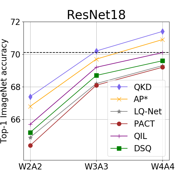
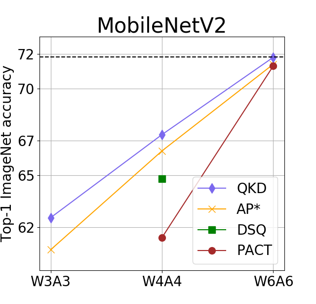
Figure 1: Top-1 accuracy on ImageNet with ResNet-18 and MobileNetV2. Our QKD is compared with various methods such as AP* [mishra2017apprentice], LQ-Net [zhang2018lq], PACT [choi2018pact], QIL [jung2019learning] and DSQ [gong2019differentiable]. Dotted line indicates the full-Precision accuracy. More details are in Table LABEL:table:standard and LABEL:table:depthwise.

Today, a majority of edge devices require fixed-point inference for compute- and power-efficiency. Hence, quantizing the weights and activations of deep networks to a certain bit-width becomes a necessity to make them compatible to edge devices. Recently, hardware accelerators like NPUs (Neural Processing Units), NVIDIA’s Tensor Core units and even CIM (Compute-in-memory) devices have targeted support for sub-byte level processing such as 4-bit$\times$4-bit or 2-bit$\times$2-bit matrix multiply-and-accumulate operations [markidis2018nvidia, pan2018multilevel, sharma2019accelerated, sumbul2019compute]. These are much more power- and compute-efficient than conventional 8-bit processing. Thus, there are increased demands for lower-bit quantization.

The accuracy of very low-bit quantized networks such as using 4-, 3- or 2-bits inevitably decreases because of their low representation power compared to typical 8-bit quantization. Some works [mishra2017apprentice, polino2018model] used knowledge distillation (KD) to improve the accuracy of quantized networks by transferring knowledge from a full-precision teacher network to a quantized student network. However, even though KD is one of the widely used techniques to enhance a DNN’s accuracy [hinton2015distilling], directly applying KD to very low-bit quantized networks incurs several challenges:

1. Due to its limited representation power, quantized networks generally show lower training and test accuracies compared to the networks with full precision. On the other hand, because KD uses not only the ground truth labels but also the teacher’s estimated class probability distributions, it acts as a heavy regularizer [hinton2015distilling]. Combining these contradictory characteristics of quantization and KD could sometimes result in further degradation of performance from that of quantization-only.

2. In general, it has been shown that a powerful teacher with high accuracy can teach a student better than a weaker one [zhu2018knowledge]. Also, [kim2018paraphrasing, mirzadeh2019improved] show that if there is a large gap from the capacity or inherent differences between the teacher and student, it can hinder the knowledge transfer because this knowledge is unadaptable to the student. Previous works of quantization with KD [mishra2017apprentice, polino2018model] directly applied conventional KD to quantization along with fixed teacher network, and thus they suffer from above mentioned limitations.

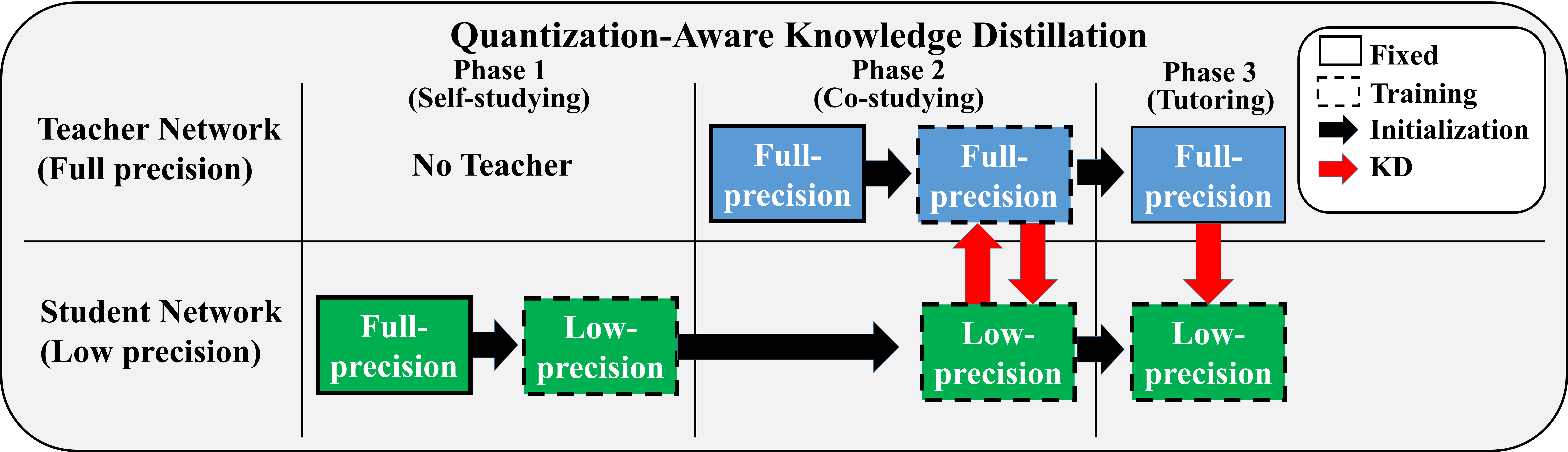
Figure 2: The overall process of QKD. Self-studying (SS) phase give a good starting point to alleviate low representative power and regularization effect of KD . Co-studying (CS) phase makes a teacher adaptable to a student and powerful than the fixed teacher. In tutoring (TU) phase, the teacher transfers its adaptable and powerful knowledge to the student.

In this paper, we propose Quantization-aware Knowledge Distillation (QKD) to address the above mentioned challenges, especially for very low-precision quantization. QKD consists of three phases. In the first ‘self-studying’ phase, instead of directly applying knowledge distillation to the quantized student network from the beginning, we first try to find a good initialization. In the second ‘co-studying’ phase, we improve the teacher by using the knowledge of the student network. This phase makes the teacher more powerful and quantization-friendly (See Section LABEL:discussion), which is essential to improve accuracy. In final ‘tutoring’ phase, we freeze the teacher network and transfer its knowledge to the student. This phase saves unnecessary training time and memory of the teacher network which tends to have already saturated in the co-studying phase. The overal process of QKD is depicted in the Figure 2. Our key contributions are the following:

• We propose Quantization-aware Knowledge Distillation which can be effectively applied to very low-bit (2-,3-,4-bit) quantized networks. Considering the characteristics of low bit networks and distillation methods, we design a combination of three phases for QKD that overcome the shortcomings posed by conventional quantization + KD methods as described above.

• We empirically verify that QKD works well on depth-wise convolution networks which are known to be difficult to quantize and our work is the first to apply KD to train low-bit depth-wise convolution networks (viz. MobileNetV2 and EfficientNet)

• We show that our QKD obtains state-of-the-art accuracies on CIFAR and ImageNet datasets compared to other existing methods. (See Figure 1.)

2 Related work

Quantization Reducing the precision of neural networks [courbariaux2015binaryconnect, li2016ternary, zhu2016trained, nagel2019data, sung2015resiliency] has been studied extensively due to its computational and storage benefits. Although binary $\{-1,+1\}$[courbariaux2015binaryconnect] or tenary $\{-1,0,+1\}$[li2016ternary] quantizations are typically used, their methods only consider the quantization of weights. To fully utilize bit-wise operations, activation maps also should be quantized in the same way as weights. Some researches consider quantizing both weights and activation maps [hubara2016binarized, soudry2014expectation, rastegari2016xnor, zhou2016dorefa, wang2019haq]. Binary neural networks [hubara2016binarized] quantize both weights and activation maps as binary and compute gradients with binary values. XNOR-Net [rastegari2016xnor] also quantizes its weights and activation maps with scaling factors obtained by constrained optimization. Furthermore, HAQ [wang2019haq] adaptively changes bit-width per layer by leveraging reinforcement learning and HW-awareness.

Recent works have tried to improve quantization further by learning the range of weights and activation maps [choi2018pact, jung2019learning, esser2019learned, uhlich2019differentiable]. These approaches can easily outperform previous methods which do not train quantization-related parameters. PACT [choi2018pact] proposes a clipping activation function using trainable a parameter which limits the maximum value of activation. LSQ [esser2019learned] and TQT [tqt2019] introduce uniform quantization using trainable interval values. QIL [jung2019learning] uses a trainable quantizer which performs both pruning and clipping. Our QKD leverages these trainable approaches in the baseline quantization implementation. On top of this quantization-only method, our elaborated knowledge distillation process boosts the accuracy, thereby achieving the state of art accuracy on low-bit quantization.

Knowledge Distillation KD is one of the most popular methods in model compression. It is widely used in many computer vision tasks. This framework transfers the knowledge of a teacher network to a smaller-sized student network in two ways: Offline and Online. First, offline KD uses a fixed pre-trained teacher networks and the knowledge transfer can happen in different ways. In [hinton2015distilling], they encourage the student network to mimic the softened distribution of the teacher network. Other works [zagoruyko2016paying, heo2019comprehensive, kim2018paraphrasing, romero2014fitnets] transfer the information using different forms of activation maps from the teacher network. Second, online KD methods [zhu2018knowledge, kim2019feature, zhang2018deep] train both the teacher and the student networks simultaneously without pre-trained teacher models. Deep Mutual Learning (DML) [zhang2018deep] have tried to transfer each knowledge of independent networks using KL loss, although it is not studied in the context of quantization. Our QKD uses both online and offline KD methods sequentially.

Quantization + Knowledge distillation Some researches have tried to use distillation methods to train low precision network [mishra2017apprentice, polino2018model]. They use a full precision network as the teacher and the low bit network as a student. In Apprentice (AP) [mishra2017apprentice], the teacher and student networks are initialized with the corresponding pre-trained full precision networks and the student is then fine-tuned using distillation. Due to AP’s initialization of the student, AP tends to get stuck in a local minimum in the case of very low-bit quantized student networks. The self-study phase of QKD directly mitigates this issue. Also, using a fixed teacher, as in [mishra2017apprentice, polino2018model], can limit the knowledge transfer due to the inherent differences between the distributions of the full-precision teacher and low-precision student network. We tackle this problem via online co-studying (CS) and offline tutoring (TU).

3 Proposed Method

In this section, we first explain the quantization method used in QKD and then describe the proposed QKD method.

3.1 Quantization

In QKD, we use a trainable uniform quantization scheme for our baseline quantization implementation. We choose uniform quantization because of its hardware-friendly characteristics. In this work, we quantize both weights and activations. So, we introduce two trainable parameters for the interval values of each layer’s weight parameters and input activations similar to [esser2019learned, tqt2019, uhlich2019differentiable]. These parameters can be trained with either the task loss or a combination of the task and distillation losses. Considering $k$-bit quantization for weights and activations, the weight and activation quantizers are defined as follows.

Weight Quantizer: Since weights can take positive as well as negative values, we quantize each weight to integers in the range $[-2^{k-1},2^{k-1}-1]$. Before rounding, the weights are first constrained to this range using a clamping function $F_{W}(w)\triangleq F(w,-2^{k-1},2^{k-1}-1)$ where

$$F(x,min,max)=\begin{cases}max&\text{if }\quad x>max\\ min&\text{if }\quad x<min\\ x&\text{elsewise}.\end{cases}$$ (1)

We use a trainable parameter $I_{W}$ for the interval value of weight quantization. It is trained along with the weights of the network. We can calculate the quantization level of the input weight $w$ using a rounding operation on $F_{W}$. The overall quantization-dequantization scheme for the weights of the network is defined as follows:

$$\hat{w}=Q_{W}(w)=\Bigl{\lfloor}{F_{W}(\frac{w}{I_{W}})+\frac{1}{2}}\Bigr{\rfloor}\times I_{W}$$ (2)

where $\lfloor\cdot\rfloor$ is the flooring operation. Note that the dequantization step (multiplication by $I_{W}$) just brings the quantized values ($\hat{w}$) back to their original range and is commonly used when emulating the effect of quantization [bhandare2019efficient, tqt2019, rodriguez2018lower].

Activation Quantizer: Since most of the networks today use ReLU as the activation function, the activation values are unsigned. Hence, to quantize the activations, we use an quantization function with the range $[0,2^{k}-1]$. The activation quantizer $Q_{X}$ can be obtained as

$$\hat{x}=Q_{X}(x)=\Bigl{\lfloor}{F_{X}(\frac{x}{I_{X}})+\frac{1}{2}}\Bigr{\rfloor}\times I_{X}$$ (3)

where, $F_{X}(x)\triangleq F(x,0,2^{k}-1)$ and $x,I_{X}$ represent activation value and the interval value of activation quantization.

Prior to training, we initialize these interval values ($I_{W}$,$I_{X}$) for every layer using the min-max values of weights and activations (form one forward pass), similar to TF-Lite [tensorflow2015-whitepaper]. These quantizers are non-differentiable, so we use a straight-through estimator (STE) [bengio2013estimating] to backprop through the quantization layer. STE approximates the gradient $\frac{d\hat{x}}{dx}$ by 1. Thus, we can approximate the gradient of loss $\mathcal{L}$, $\frac{d\mathcal{L}}{dx}$, with $\frac{d\mathcal{L}}{d\hat{x}}$

$$\frac{d\mathcal{L}}{dx}=\frac{d\mathcal{L}}{d\hat{x}}\frac{d\hat{x}}{dx}\approx\frac{d\mathcal{L}}{d\hat{x}}.$$ (4)

3.2 Quantization-aware Knowledge Distillation

We will now describe the three phases of QKD. Algorithm 1 depicts the overall QKD training process.

3.2.1 Phase 1: Self-studying

Directly combining quantization and KD cannot make the most of the positive effects of KD and easily cause unexpectedly lower performance. This is because of the regularizing characteristics of KD and limited representative power of the quantized network. This can cause the quantized network to easily get trapped in a poor local minima. To mitigate this issue and to provide a good starting point for KD, we train the low-bit network for some epochs using only the task loss, i.e. the standard cross entropy loss. Such a self-studying phase provides the student with good initial parameters before KD is applied.

Our method can be compared to progressive quantization (PQ) [zhuang2018towards] which also uses two stages and progressively quantizes weights and activation maps for a good initial point. While PQ conducts progressive quantization which uses a higher precision network as a initialization and conducts iterative update between weight and activation maps, our method directly initializes the same low bit-width for the target low-bit network because learning the interval of weights and activation maps works well without iterative and progressive training.

This strategy of parameter initialization and knowledge distillation has good synergy in terms of generalization and finding a good local minimum. More specifically, our initialization scheme helps to start with a good starting point and the distillation loss guides the student network to good local minima acting as a regularizer.

Algorithm 1 Quantization-aware Knowledge Distillation

0:  Training data; Pre-trained FP weights for teacher model $T_{F}$; Pre-trained FP weights for student model $S_{F}$; Low-bit student model weights ${S_{L}}$; Weight interval values $I_{W}$; Activation interval values $I_{X}$; Number of epochs for each phase $P_{1}$; $P_{2}$; $P_{3}$;

0:  Trained low-bit student weight and interval values ${S_{L}}^{\prime}$, ${I_{W}}^{\prime}$ and ${I_{X}}^{\prime}$

1:  Phase 1: Self-studying

2:  Init $S_{L}$ with $S_{F}$; Init $I_{W},I_{X}$ using min-max values of weights and one batch of activations;

3:  for  Epoch = 1 ,…, $P_{1}$ do

4:     Update $S_{L}$, $I_{W}$ and $I_{X}$ by minimizing $\mathcal{L}^{s}_{ce}$ (6)

5:  end for

6:  Phase 2: Co-studying

7:  Init ${S_{L}}^{\prime}$, ${I_{W}}^{\prime}$ and ${I_{X}}^{\prime}$ with $S_{L}$, $I_{W}$ and $I_{X}$

8:  for  Epoch = 1 ,…, $P_{2}$ do

9:     Update $T_{F}$ by minimizing $\mathcal{L}^{T}_{KD}$ (9)

10:     Update ${S_{L}}^{\prime}$, ${I_{W}}^{\prime}$ and ${I_{X}}^{\prime}$ by minimizing $\mathcal{L}^{S}_{KD}$ (8)

11:  end for

12:  Phase 3: Tutoring

13:  for  Epoch = $1$ ,…, $P_{3}$ do

14:     Update ${S_{L}}^{\prime}$, ${I_{W}}^{\prime}$ and ${I_{X}}^{\prime}$ by minimizing $\mathcal{L}^{S}_{KD}$ (8)

15:  end for

3.2.2 Phase 2: Co-studying

To make a powerful and adaptable teacher, we jointly train the teacher network (full-precision) and the student network (low-precision) in an online manner. Kullback–Leibler divergence (KL) between the student and teacher distributions is used to the make the teacher more powerful in terms of accuracy as well as it’s adaptability to the student distribution than the fixed pre-trained teacher. In this framework, teacher network is trained by softened distribution of student network and vice versa. Teacher network can be adapted to the quantized student network with KL loss by awaring the distribution of the quantized network.

Assuming that there are $m$ classes, the cross-entropy loss for both the teacher and the student networks is obtained by firstly computing the softmax posterior with temperature $\mathcal{T}$ as follows:

$$p_{i}(\mathbf{z}^{k};\mathcal{T})=\frac{e^{z^{k}_{i}/\mathcal{T}}}{\sum_{j}^{m}e^{z^{k}_{j}/\mathcal{T}}},$$ (5)

$$\mathcal{L}_{ce}^{k}=-\sum_{i=1}^{m}y^{(i)}\log(p_{i}(\mathbf{z}^{k};1)),$$ (6)

where $\mathbf{z}^{k}$ and $\mathcal{L}_{ce}^{k}$ represent logit and cross-entropy of the $k$-th network, i.e. the student or the teacher ($k=\{S,T\}$). The temperature value, $\mathcal{T}$, is used to make distribution softer for using the dark knowledge. We can compute the KL loss between student and teacher network using logits.

$${KL}(z^{T}||z^{S};\mathcal{T})=\sum_{i=1}^{m}p_{i}(z^{T};\mathcal{T})\log(\frac{p_{i}(z^{T};\mathcal{T})}{p_{i}(z^{S};\mathcal{T})}).$$ (7)

Then, we update each network with cross entropy and KL loss as below:

$$\mathcal{L}^{S}_{KD}=\mathcal{L}_{ce}^{S}+\mathcal{T}^{2}\times{KL}(z^{T}||z^{S};\mathcal{T})$$ (8)

$$\mathcal{L}^{T}_{KD}=\mathcal{L}_{ce}^{T}+\mathcal{T}^{2}\times{KL}(z^{S}||z^{T};\mathcal{T})$$ (9)

$\mathcal{L}^{S}_{KD}$ and $\mathcal{L}^{S}_{KD}$ refer to the loss of student and teacher network, respectively. We multiply $\mathcal{T}^{2}$ because the gradient scale of logits decrease as much as $1/\mathcal{T}^{2}$.

3.2.3 Phase 3: Tutoring

After a few epochs of co-studying, the accuracy of teacher network starts saturating. This is because the teacher (full-precision) has relatively high representative power than the student (low-precision). To reduce the computational cost and memory in calculating the gradient of the teacher network, we freeze the teacher network and train only the low-bit student network with $\mathcal{L}^{S}_{KD}$ loss in an offline manner. In this phase, we use the knowledge of a teacher network which is now more quantization-aware as a result of co-studying. As we will show later (See Section LABEL:discussion), using tutoring gives us equal or better student performance compared to only using co-studying throughout the training.

4 Experiments

We perform a comprehensive evaluation of our method on the CIFAR10/100 [krizhevsky2009learning] and ImageNet [ILSVRC15] datasets. We compare the proposed QKD with existing state-of-the-art quantization methods on 2, 3, and 4-bits (i.e., W2A2, W3A3, W4A4). To show the robustness of our method, we provide comparisons on standard convolutions (i.e., ResNet [he2016deep]) as well as depth-wise separable convolutions (i.e., MobileNetV2 [sandler2018mobilenetv2] and EfficientNet [tan2019efficientnet]). Furthermore, we perform an extensive ablation study to analyze the effectiveness of the different components of QKD. Following methods are considered for performance comparison:

1. ‘Baseline (BL)’ is the baseline quantization-only version of QKD as described in 3.1; no teacher is used during training. We train the low precision network using cross-entropy and initialize the weights with the pretrained full-precision weights.

2. ‘SS + BL’ is BL, but the low-bit betwork is initialized with the weights and interval values trained in the self-studying (SS) phase.

3. ‘AP*’ is a modified version of the original Apprentice [mishra2017apprentice] method for knowledge distillation. The original Apprentice uses WRPN scheme [mishra2017wrpn]. We replace this quantizer with BL and initialize both teacher and student with pre-trained full-precision newtork.

4. ‘SS + AP*’ is AP* initialized with the weights and interval values trained in the self-studying (SS) phase for the low-precision network.

5. ‘CS + TU’ means that we initialize the student network with pre-trained full-precision network the same way as AP*, then perform “Co-studying” and “Tutoring” between the teacher and the student using BL.

6. ‘QKD (SS + CS + TU)’ is our proposed method. We initialize the student network by the SS phase. Then, we perform KD in the CS + TU phase.

4.1 Implementation Details

We quantize the weights and input activations of all the Conv and Linear layers as described in Section 3.1. We quantize first and last layer to 8-bits to ensure compatibility on any fixed-point hardware. We set the temperature value $\mathcal{T}$ as 2 in QKD. In all the experiments, we use the same settings while training all 6 baselines mentioned above.

CIFAR We train for up to $200$ epochs with step learning rate schedule with SGD same as [zhang2018lq]. We use the starting learning rate (LR) of $0.1$ and $0.01$ for models corresponding to CIFAR-10/100 respectively. We use 30 epochs for SS phase by dividing LR with $10$ for every 10 epoch. After SS phase, we reset the LR to $0.1$ and $0.01$ corresponding to CIFAR-10/100. Then, we use other 170 epochs for CS + TU phase. LR learning rate is divided by $10$ at $80$ and $120$ epoch. We use 100 epochs for CS and the remaining 70 epochs for TU. For teacher network, we use the same schedule as the student for the CS phase, but we freeze the teacher in TU. Compared to the LR used for student model’s weight parameters, we use 100 times smaller LR for updating $I_{W}$ and same LR for updating $I_{X}$.

ImageNet For all our compared methods, we used total 120 epochs for training (this is the same length as QIL [jung2019learning]). In the methods SS + BL, SS + AP* and SS + CS + TU, we finetune the student model for 50 epochs in the SS phase and the remaining 70 epochs are used for the rest. In the CS + TU method, the first 60 epochs are for CS and the remaining 60 epochs for TU. For training the student, we used a Mixed Optimizer (MO) setting [opennmt]. In the MO setting, we use SGD [bottou2010large] optimizer to update the weights and Adam [kingma2014adam] for updating the interval values ($I_{W}$, $I_{X}$). We found that the exponential learning rate schedule works best for QKD. For the ResNet architectures, we use an initial learning rate of $0.001$ for both SS and CS + TU phases. For EfficientNet and MobileNetV2, initial learning rate of $0.003$ was used. Similar to CIFAR-100 setting, we use 100 times smaller LR for $I_{W}$ and same LR for $I_{X}$, compared to LR for model weights. For $I_{W}$ and $I_{X}$, not much fine-tuning was required because of the Mixed Optimizer setting. More details are described in supplementary details.

4.2 CIFAR-10 Results

We evaluate our method on the CIFAR-10 dataset. The performance numbers are shown in the Table LABEL:table:cifar10. We use ResNet-56 (FP : 93.4%) as a teacher network for both AP* and QKD. Interestingly, for AP* and CS + TU, which combine BL and knowledge distillation, performance is worse than BL at W2A2. This is because the network has low-representative power at W2A2 and can be negatively affected by the heavy regularization imposed by KD. To alleviate this issue, we use the weights trained in the SS phase for a better initialization for the weights of the student. SS + AP* and QKD outperform the existing methods and the Baseline (BL) method for all the cases. These results suggest that initialization is very important in combining quantization and any KD method. In our proposed method, 2% gain was observed at W2A2 with the SS phase. Compared to the distillation method AP*, QKD which also trains the teacher shows a significant improvement in performance. QKD also provides best results for W3A3 and W4A4.

Table 1: CIFAR-10 top-1 accuracy