The bivariate $K$-finite normal mixture “blanket” copula

Abstract

There exist many bivariate parametric copulas to model bivariate data with different dependence features. We propose a new bivariate parametric copula family that cannot only handle various dependence patterns that appear in the existing parametric bivariate copula families, but also provides a more enriched dependence structure. The proposed copula construction exploits finite mixtures of bivariate normal distributions. The mixing operation, the distinct correlation and mean parameters at each mixture component introduce quite a flexible dependence. The new parametric copula is theoretically investigated, compared with a set of classical bivariate parametric copulas and illustrated on two empirical examples from astrophysics and agriculture where some of the variables have peculiar and asymmetric dependence, respectively.

Key Words: Bivariate copulas; Dependence structure; Kullback-Leibler distance; Mixtures of bivariate normal distributions.

1 Introduction

Multivariate response data abound in many applications including insurance, risk management, finance, health and environmental sciences. Data from these application areas have different dependence structures including features such as tail dependence (Joe,, 1993), that is dependence among extreme values. Modelling dependence among multivariate outcomes is an interesting problem in statistical science. The dependence between random variables is completely described by their multivariate distribution. One may create multivariate distributions based on particular assumptions thus, limiting their use. For example, most existing multivariate distributions assume margins of the same form (e.g., Gaussian, Poisson, etc.) or limited dependence (e.g., tail independence, positive dependence, etc.).

To solve this problem, copula functions (Joe,, 1997, 2014; Nelsen,, 2006) seem to be a promising solution. The power of copulas for dependence modelling is due to the dependence structure being considered separate from the univariate margins. Copulas are a useful way to model multivariate data as they account for the dependence structure and provide a flexible representation of the multivariate distribution. They allow for flexible dependence modelling, different from assuming simple linear correlation structures and normality, which makes them well suited to the aforementioned application areas. In particular, the theory and application of copulas have become important in finance, insurance and other areas, in order to deal with dependence in the joint tails (Joe et al.,, 2010).

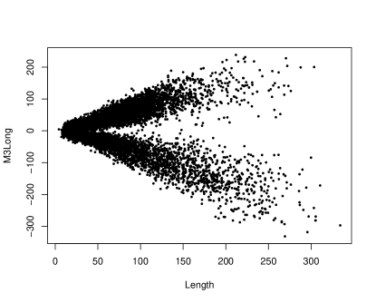
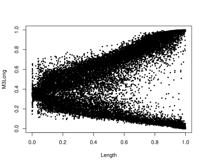
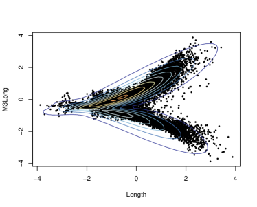
For the bivariate case, a rich variety of copula families is available and their properties are well-established (Joe,, 1997, 2014; Nelsen,, 2006). Nevertheless, a problem in practical applications is to identify the most plausible parametric family of bivariate copulas for dependence modelling (Durrleman et al.,, 2000; Huard et al.,, 2006; Nikoloulopoulos and Karlis,, 2008). Furthermore, sometimes none of the bivariate parametric copula families provides a good fit. For example, Nagler and Czado, (2016) and Czado, (2019) analysed the dependence between the Major Atmospheric Gamma Imaging Cherenkov (MAGIC) telescope variables (Bock et al.,, 2004) and pointed out the uncommon characteristics of the dependence structure between some of the variables, which do not correspond to any bivariate parametric copula. Figure 1 depicts, in particular the relationship between the length of the major axis of the ellipse (Length) and the third root of the third moment along the major axis (M3Long), and indeed reveals that none of the existing parametric families of bivariate copulas (see e.g., Joe, 1997, 2014) can model the joint distribution of these variables. Note in passing that in the right panel graph of Figure 1, we transform the data to the uniform scale by applying their empirical distributions, in order to isolate the effect of the marginal distributions and solely focus on the dependence structure.

Figure 1: Scatter plots of the length of the major axis of the ellipse (Length) and the third root of the third moment along the major axis (M3Long) on the original and uniform scale.

In this paper, we propose a new parametric family of copulas that can represent the dependence structure between the aforementioned MAGIC variables. It can also remedy the copula selection issue as can “nearly” approximate any parametric family of bivariate copulas. A multivariate 2-finite normal mixture (FNM) copula has been proposed by Nikoloulopoulos and Karlis, (2009) to model multivariate discrete data. The correlation matrix for each mixture component was restricted to the identity matrix with the mixing operation introducing the dependence among the discrete responses. Therefore, it has a rather simple computational form, but suffers from a restricted range of attainable dependence. We will study the full dependence capacity of the bivariate $K$-FNM copula, where $K$ is the number of mixture components, by using general correlation matrices for each mixture component and we will show that the the proposed $K$-FNM is a “blanket” copula, i.e., a copula that can “nearly” approximate any bivariate parametric copula. A similar construction in the literature, which is called Bayesian non-parametric estimation of a copula (Wu et al.,, 2015; Dalla Valle et al.,, 2018), takes BVN copulas as the mixture components, hence it allows only for reflection symmetric dependence and is not as general as the proposed $K$-FNM copula, which can allow reflection asymmetric dependence.

The remainder of the paper proceeds as follows. Section 2 introduces the bivariate $K$-FNM copula, discusses its properties and provides computational details for maximum likelihood (ML) estimation. Before that it has a brief overview of relevant copula theory. Section 3 shows that the proposed copula is a “blanket” copula. Section 4 studies the small-sample efficiency of the proposed ML estimation technique. Section 5 illustrates the methods on two empirical examples from astrophysics and agriculture where some of the variables have peculiar and asymmetric dependence, respectively. We conclude with some discussion in Section 6.

2 The bivariate $K$-finite normal mixture copula

In this section we will define the bivariate $K$-FNM copula and study its properties. Before that, the first subsection has some background on bivariate copulas.

2.1 Overview and relevant background for copulas

A copula is a multivariate cumulative distribution function (cdf) with uniform $U(0,1)$ margins (Joe,, 1997; Nelsen,, 2006; Joe,, 2014). If $F_{12}$ is a bivariate cdf with univariate margins $F_{1},F_{2}$, then Sklar’s (1959) theorem implies that there is a copula $C$ such that

$$F_{12}(y_{1},y_{2})=C\Bigl{(}F_{1}(y_{1}),F_{2}(y_{2})\Bigr{)}.$$

The copula is unique if $F_{1},F_{2}$ are continuous, but not if some of the $F_{j}$ have discrete components. If $F_{12}$ is continuous and $(Y_{1},Y_{2})\sim F_{12}$, then the unique copula is the distribution of $(U_{1},U_{2})=\left(F_{1}(Y_{1}),F_{2}(Y_{2})\right)$ leading to

$$C(u_{1},u_{2})=F_{12}\Bigl{(}F_{1}^{-1}(u_{1}),F_{2}^{-1}(u_{2})\Bigr{)},\quad 0\leq u_{j}\leq 1,j=1,2,$$ (1)

where $F_{j}^{-1}$ are inverse cdfs. In particular, if $\Phi_{12}(\cdot;\theta)$ is the bivariate normal (BVN) cdf with correlation $\theta$ and standard normal margins, and $\Phi$ is the univariate standard normal cdf, then the BVN copula is

$$C(u_{1},u_{2})=\Phi_{12}\Bigl{(}\Phi^{-1}(u_{1}),\Phi^{-1}(u_{2});\theta\Bigr{)}.$$ (2)

If $C(\cdot;\theta)$ is a parametric family of copulas and $F_{j}(\cdot;\eta_{j})$ is a parametric model for the $j$th univariate margin, then

$$C\Bigl{(}F_{1}(y_{1};\eta_{1}),F_{2}(y_{2};\eta_{2});\theta\Bigr{)}$$

is a bivariate parametric model with univariate margins $F_{1},F_{2}$. For copula models, the variables can be continuous or discrete (Nikoloulopoulos,, 2013; Nikoloulopoulos and Joe,, 2015).

2.2 The bivariate $K$-FNM copula

Let a bivariate $K$-FNM distribution be defined as

$$\sum_{k=1}^{K}\pi_{k}{\mathcal{N}}_{2}(\boldsymbol{\mu}_{k},\mathbf{\Sigma}_{k}),\quad 0<\pi_{k}<1,\quad\sum_{k=1}^{K}\pi_{k}=1,$$

where ${\mathcal{N}}_{2}(\boldsymbol{\mu},\mathbf{\Sigma})$ denotes the BVN distribution with mean vector $\boldsymbol{\mu}=(\mu_{1},\mu_{2})$ and covariance matrix $\mathbf{\Sigma}=\begin{pmatrix}\sigma_{1}^{2}&\rho\sigma_{1}\sigma_{2}\\ \rho\sigma_{1}\sigma_{2}&\sigma_{2}^{2}\end{pmatrix}$. Its cdf is given by

$$\mathcal{F}_{2}(\mathbf{y};\pi_{k},\boldsymbol{\mu}_{k},\mathbf{\Sigma}_{k},\,k=1,\ldots,K)=\sum_{k=1}^{K}\pi_{k}\Phi_{2}(\mathbf{y};\boldsymbol{\mu}_{k},\mathbf{\Sigma}_{k}),\quad 0<\pi_{k}<1,\quad\sum_{k=1}^{K}\pi_{k}=1,$$ (3)

where $\Phi_{2}(\mathbf{y};\boldsymbol{\mu},\mathbf{\Sigma})$ is the cdf of the ${\mathcal{N}}_{2}(\boldsymbol{\mu},\mathbf{\Sigma})$ distribution.

From (1) if $F_{12}$ is the bivariate $K$-FNM cdf $\mathcal{F}_{2}$ in (3) and $F_{1}=F_{2}=\mathcal{F}$, where $\mathcal{F}$ is the univariate $K$-FNM cdf, then the bivariate $K$-FNM copula is defined as

$$C(u_{1},u_{2};\pi_{k},\boldsymbol{\mu}_{k},\mathbf{\Sigma}_{k},\,k=1,\ldots,K)=\\ \mathcal{F}_{2}\Bigl{(}\mathcal{F}^{-1}(u_{1};\pi_{k},\mu_{k1},\sigma_{k1},\,k=1,\ldots,K),\mathcal{F}^{-1}(u_{2};\pi_{k},\mu_{k2},\sigma_{k2},\,k=1,\ldots,K);\pi_{k},\boldsymbol{\mu}_{k},\mathbf{\Sigma}_{k},\,k=1,\ldots,K\Bigr{)}.$$ (4)

Subsequently, one can derive the bivariate $K$-FNM copula density as below

$$c(u_{1},u_{2};\pi_{k},\boldsymbol{\mu}_{k},\mathbf{\Sigma}_{k},\,k=1,\ldots,K)=\\ \frac{{f}_{2}\Bigl{(}\mathcal{F}^{-1}(u_{1};\pi_{k},\mu_{k1},\sigma_{k1},\,k=1,\ldots,K),\mathcal{F}^{-1}(u_{2};\pi_{k},\mu_{k2},\sigma_{k2},\,k=1,\ldots,K);\pi_{k},\boldsymbol{\mu}_{k},\mathbf{\Sigma}_{k},\,k=1,\ldots,K\Bigr{)}}{f\Bigl{(}\mathcal{F}^{-1}(u_{1};\pi_{k},\mu_{k1},\sigma_{k1},\,k=1,\ldots,K)\Bigr{)}f\Bigl{(}\mathcal{F}^{-1}(u_{2};\pi_{k},\mu_{k2},\sigma_{k2},\,k=1,\ldots,K)\Bigr{)}},$$ (5)

where $f$ and $f_{2}$ is the univariate and bivariate density, respectively, of the $K$-FNM distribution.

2.3 Dependence properties of the $K$-FNM distribution

We study the dependence properties of the bivariate $K$-FNM distribution as these will be inherited to the copula. The mean vector and covariance matrix of the $K$-FNM are given respectively by

$$\boldsymbol{\mu}=\sum_{k=1}^{K}\pi_{k}\boldsymbol{\mu}_{k}\quad\mbox{and}\quad\boldsymbol{\Delta}=\sum_{k=1}^{K}\pi_{k}\mathbf{\Sigma}_{k}+\sum_{k=1}^{K}\pi_{k}\boldsymbol{\mu}_{k}\boldsymbol{\mu}_{k}^{\top}-\boldsymbol{\mu}\boldsymbol{\mu}^{\top}.$$

An aspect of mixture models is their lack of identifiability, but this can be overcome by imposing some restrictions in the parameters. In our approach, to overcome the typical identifiability issues we priory assume that $\boldsymbol{\mu}_{1}+\ldots+\boldsymbol{\mu}_{K}={\bf 0}$, i.e., the mean vectors become

$$\boldsymbol{\mu}_{1}=(\nu_{1},\nu_{2}),\ldots,\boldsymbol{\mu}_{K-1}=(\nu_{2K-3},\nu_{2K-2}),\boldsymbol{\mu}_{K}=(-\sum_{k=1}^{K-1}\nu_{2k-1},-\sum_{k=1}^{K-1}\nu_{2k}),$$

and that the variances of the mixture components are set to one, i.e., $\sigma_{k1}^{2}=\sigma_{k2}^{2}=1$ for $k=1,\ldots,K$.

The covariance matrix is then of the form $\boldsymbol{\Delta}=\begin{pmatrix}\Delta_{11}&\Delta_{12}\\ \Delta_{12}&\Delta_{22}\end{pmatrix},$ where

$$\Delta_{11}=1+\sum_{k=1}^{K-1}\pi_{k}\nu_{2k-1}^{2}+\pi_{K}\Bigl{(}\sum_{k=1}^{K-1}\nu_{2k-1}\Bigr{)}^{2}-\Bigl{(}\sum_{k=1}^{K-1}\pi_{k}\nu_{2k-1}-\pi_{K}\sum_{k=1}^{K-1}\nu_{2k-1}\Bigr{)}^{2},$$

$$\Delta_{12}=\sum_{k=1}^{K-1}\pi_{k}\nu_{2k-1}\nu_{2k}+\pi_{K}\sum_{k=1}^{K-1}\nu_{2k-1}\sum_{k=1}^{K-1}\nu_{2k}-\Bigl{(}\sum_{k=1}^{K-1}\pi_{k}\nu_{2k-1}-\pi_{K}\sum_{k=1}^{K-1}\nu_{2k-1}\Bigr{)}\Bigl{(}\sum_{k=1}^{K-1}\pi_{k}\nu_{2k}-\pi_{K}\sum_{k=1}^{K-1}\nu_{2k}\Bigr{)}+\sum_{k=1}^{K}\pi_{k}\rho_{k},$$

and

$$\Delta_{22}=1+\sum_{k=1}^{K-1}\pi_{k}\nu_{2k}^{2}+\pi_{K}\Bigl{(}\sum_{k=1}^{K-1}\nu_{2k}\Bigr{)}^{2}-\Bigl{(}\sum_{k=1}^{K-1}\pi_{k}\nu_{2k}-\pi_{K}\sum_{k=1}^{K-1}\nu_{2k}\Bigr{)}^{2}.$$

As one can easily see, an identifiability problem still occurs. To overcome this, we set $\nu_{1}=K-1,\nu_{3}=\cdots=\nu_{2K-3}=-1$ and $\nu_{2}=\theta_{1},\nu_{4}=\theta_{2},\ldots,\nu_{2K-2}=\theta_{K-1}$.

Accordingly, the variance-covariance terms of $\boldsymbol{\Delta}$ reduce to

$$\Delta_{11}=1+\pi_{1}(1-\pi_{1})K^{2},$$

$$\Delta_{12}=\pi_{1}\theta_{1}(K-1)-\sum_{k=2}^{K-1}\pi_{k}\theta_{k}+\pi_{K}\sum_{k=1}^{K-1}\theta_{k}+(1-\pi_{1}K)\Bigl{(}\sum_{k=1}^{K-1}\pi_{k}\theta_{k}-\pi_{K}\sum_{k=1}^{K}\theta_{k}\Bigr{)}+\sum_{k=1}^{K}\pi_{k}\rho_{k},$$

and

$$\Delta_{22}=1+\sum_{k=1}^{K-1}\pi_{k}\theta_{k}^{2}+\pi_{K}\Bigl{(}\sum_{k=1}^{K-1}\theta_{k}\Bigr{)}^{2}-\Bigl{(}\sum_{k=1}^{K-1}\pi_{k}\theta_{k}-\pi_{K}\sum_{k=1}^{K-1}\theta_{k}\Bigr{)}^{2}.$$

The Pearson’s correlation parameter is

$$\rho=\frac{\pi_{1}\theta_{1}(K-1)-\sum_{k=2}^{K-1}\pi_{k}\theta_{k}+\pi_{K}\sum_{k=1}^{K-1}\theta_{k}+(1-\pi_{1}K)\Bigl{(}\sum_{k=1}^{K-1}\pi_{k}\theta_{k}-\pi_{K}\sum_{k=1}^{K}\theta_{k}\Bigr{)}+\sum_{k=1}^{K}\pi_{k}\rho_{k}}{\sqrt{1+\pi_{1}(1-\pi_{1})K^{2}}\sqrt{1+\sum_{k=1}^{K-1}\pi_{k}\theta_{k}^{2}+\pi_{K}\Bigl{(}\sum_{k=1}^{K-1}\theta_{k}\Bigr{)}^{2}-\Bigl{(}\sum_{k=1}^{K-1}\pi_{k}\theta_{k}-\sum_{k=1}^{K-1}\theta_{k}\Bigr{)}^{2}}}$$

and can attain the $\pm 1$ values.

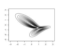
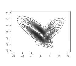
We depict some dependence shapes that can be imposed by the bivariate $K$-FNM copula with the above parametrization in Figure 2.

$K=2\quad\pi_{1}=0.3\quad\rho_{1}=0.8\quad\rho_{2}=-0.8$
$\theta_{1}=-1.5$	$\theta_{1}=0$	$\theta_{1}=1.5$
$K=3\quad\rho_{1}=0.8\quad\rho_{2}=-0.8\quad\rho_{3}=0.8\quad\pi_{1}=0.2\quad\pi_{2}=0.5$
$\theta_{1}=\theta_{2}=-1.5$	$\theta_{1}=\theta_{2}=0$	$\theta_{1}=\theta_{2}=1.5$

Figure 2: Contour plots of the $K$-FNM copula with $K=2$ (upper panel) and $K=3$ (lower panel) components and standard normal margins for various parametrizations.

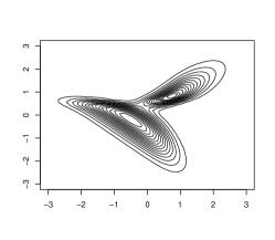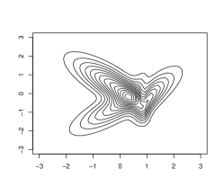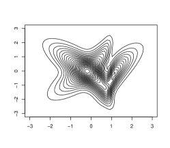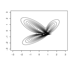2.4 Maximum likelihood estimation

In copula models, a copula is combined with a set of univariate margins. This is equivalent to assuming that variables $Y_{1},Y_{2}$ have been transformed to uniform random variables $U_{1}=F_{1}(Y_{1}),U_{2}=F_{2}(Y_{2})$. For data $y_{ij},\,i=1,\ldots,n,\,j=1,2$, we use either non-parametric or parametric univariate distributions to transform the data $y_{ij}$ to copula data $u_{ij}=F_{j}(y_{ij})$, i.e., data on the uniform scale. These semi-parametric and parametric estimation techniques have been developed by Genest et al., (1995) and Joe, (2005), respectively, and can be regarded as two-step approaches on the original data or simply as the standard one-step maximum likelihood (ML) method on the transformed (copula) data.

To this end, estimation of the $K$-FNM copula parameters $(\pi_{1},\ldots,\pi_{K-1},\theta_{1},\ldots,\theta_{K-1},\rho_{1},\ldots,\rho_{K})$ can be approached by maximizing the logarithm of the joint likelihood

$$\ell(\pi_{1},\ldots,\pi_{K-1},\theta_{1},\ldots,\theta_{K-1},\rho_{1},\ldots,\rho_{K})=\sum_{i=1}^{N}\log\Bigl{(}c(u_{i1},u_{i2};\pi_{1},\ldots,\pi_{K-1},\theta_{1},\ldots,\theta_{K-1},\rho_{1},\ldots,\rho_{K})\Bigr{)},$$

where $c(\cdot;\cdot)$ is the $K$-FNM copula density given in (5). The estimated parameters can be obtained by using a quasi-Newton (Nash,, 1990) method applied to the logarithm of the joint likelihood. This numerical method requires only the objective function, i.e., the logarithm of the joint likelihood, while the gradients are computed numerically and the Hessian matrix of the second order derivatives is updated in each iteration. The standard errors (SE) of the ML estimates can be also obtained via the gradients and the Hessian computed numerically during the maximization process.

3 Is the bivariate $K$-FNM a “blanket” copula?

In this section we will show that the $K$-FNM copula is quite close to any parametric family of copulas. We will use the Kullback-Leibler methodology (Joe,, 2014, pages 234-241) to compare the new parametric copula family with existing parametric families of copulas. Before that, the first subsection provides choices of parametric bivariate copulas.

3.1 Existing parametric families of copulas

We will consider copula families that have different tail dependence (Joe,, 1993) or tail order (Hua and Joe,, 2011). A bivariate copula $C$ is reflection symmetric if its density satisfies $c(u_{1},u_{2})=c(1-u_{1},1-u_{2})$ for all $0\leq u_{1},u_{2}\leq 1$. Otherwise, it is reflection asymmetric often with more probability in the joint upper tail or joint lower tail. Upper tail dependence means that $c(1-u,1-u)=O(u^{-1})$ as $u\to 0$ and lower tail dependence means that $c(u,u)=O(u^{-1})$ as $u\to 0$. If $(U_{1},U_{2})\sim C$ for a bivariate copula $C$, then $(1-U_{1},1-U_{2})\sim\widehat{C}$, where $\widehat{C}(u_{1},u_{2})=u_{1}+u_{2}-1+C(1-u_{1},1-u_{2})$ is the survival or reflected copula of $C$; this “reflection” of each uniform $U(0,1)$ random variable about $1/2$ changes the direction of tail asymmetry. Under some regularity conditions (e.g., existing finite density in the interior of the unit square, ultimately monotone in the tail), if there exists $\kappa_{L}(C)>0$ and some $L(u)$ that is slowly varying at $0^{+}$ (i.e., $\frac{L(ut)}{L(u)}\sim 1,$ as $u\to 0^{+}$ for all $t>0$), then $\kappa_{L}(C)$ is the lower tail order of $C$. The upper tail order $\kappa_{U}(C)$ can be defined by the reflection of $(U_{1},U_{2})$, i.e., ${\overline{C}}(1-u,1-u)\sim u^{\kappa_{U}(C)}L^{*}(u)$ as $u\to 0^{+}$, where ${\overline{C}}$ is the survival function of the copula and $L^{*}(u)$ is a slowly varying function. With $\kappa=\kappa_{L}$ or $\kappa_{U}$, a bivariate copula has intermediate tail dependence if $\kappa\in(1,2)$, tail dependence if $\kappa=1$, and tail quadrant independence if $\kappa=2$ with $L(u)$ being asymptomatically a constant.

After briefly providing definitions of tail dependence and tail order we provide below a list of bivariate parametric copulas with varying tail behaviour:

• Reflection symmetric copulas with intermediate tail dependence such as the BVN copula in (2) with $\kappa_{L}=\kappa_{U}=2/(1+\theta)$, where $\theta$ is the copula (correlation) parameter.

• Reflection symmetric copulas with tail quadrant independence ($\kappa_{L}=\kappa_{U}=2$), such as the Frank copula.

• Reflection asymmetric copulas with upper tail dependence only such as the Gumbel copula with $\lambda_{L}=0$ ($\kappa_{L}=2^{1/\theta}$) and $\lambda_{U}=2^{1/\theta}$ ($\kappa_{U}=1$), where $\theta$ is the copula parameter.

• Reflection asymmetric copulas with lower tail dependence only such as the Clayton copula with $\lambda_{L}=2^{-1/\theta}$ ($\kappa_{L}=1$) and $\lambda_{U}=0$ ($\kappa_{U}=2$), where $\theta$ is the copula parameter.

• Reflection symmetric copulas with tail dependence, such as the $t_{\nu}$ copula with $\lambda=\lambda_{L}=\lambda_{U}=2T_{\nu+1}\Bigl{(}-\sqrt{(\nu+1)(1-\theta)/(1+\theta)}\Bigr{)}$ ($\kappa_{L}=\kappa_{U}=1$), where $\theta$ is the correlation parameter of the bivariate $t$ distribution with $\nu$ degrees of freedom, and $T_{\nu}$ is the univariate $t$ cdf with $\nu$ degrees of freedom.

• Reflection asymmetric copulas with upper and lower tail dependence that can range independently from 0 to 1, such as the BB1 copula with $\lambda_{L}=2^{-1/(\theta\delta)}$ ($\kappa_{L}=1$) and $\lambda_{U}=2-2^{1/\delta}$ ($\kappa_{U}=1$) or the BB7 copula with $\lambda_{L}=2^{-1/\delta}$ ($\kappa_{L}=1$) and $\lambda_{U}=2^{1/\theta}$ ($\kappa_{U}=1$), where $\theta$ and $\delta$ are the copula parameters.

The aforementioned bivariate copula families are sufficient for applications because tail dependence and tail order are properties to consider when choosing amongst different families of copulas, and the concepts of upper/lower tail dependence and upper/lower tail order are one way to differentiate families. Nikoloulopoulos and Karlis, (2008) and Joe, (2014) have shown that it is hard to choose a copula with similar tail dependence properties from real data because copulas with similar tail dependence properties provide similar fit.

3.2 Kullback-Leibler distance and sample size

For inferences based on likelihood, the Kullback-Leibler (KL) distance is relevant, especially as the parametric model used in the likelihood could be misspecified (Joe,, 2014). Typically, one considers several different models when analysing data, and from a theoretical point of view, the KL distance of pairs of competing models provides information on the sample size needed to discriminate them.

We will define the KL distance for two copula densities and the expected log-likelihood ratio. Because the KL is a non-negative quantity that is not bounded above, we use also the expected value of the square of the log-likelihood ratio in order to get a sample size value that is an indication of how different two copula densities are. Consider two copula densities (competing models) $c_{1}$ and $c_{2}$ with respect to Lebesgue or counting measure in $\mathbb{R}^{2}$. The KL distance between copulas with densities $c_{1},c_{2}$ is defined as

$$\mbox{KL}(c_{1},c_{2})=E_{c_{1}}\left[\log\left(\frac{c_{1}(u_{1},u_{2})}{c_{2}(u_{1},u_{2})}\right)\right]=\int_{0}^{1}\int_{0}^{1}\log\left(\frac{c_{1}(u_{1},u_{2})}{c_{2}(u_{1},u_{2})}\right)c_{1}(u_{1},u_{2})du_{1}du_{2}.$$ (6)

The KL distance can be interpreted as the average difference of the contribution to the log-likelihood of one observation.

We use the log-likelihood ratio to get a sample size $n_{c_{1},c_{2}}$ which gives an indication of the sample size needed to distinguish $c_{1}$ and $c_{2}$ with probability at least 0.95. If $c_{1},c_{2}$ are similar, then $c_{1},c_{2}$ will be larger, and if $c_{1},c_{2}$ are far apart, then $n_{c_{1},c_{2}}$ will be smaller. The calculation is based on an approximation from the Central Limit Theorem and assumes that the square of the log-likelihood ratio has finite variance when computed with $c_{1}$ being the true density (Joe,, 2014). If the variance of the log-density ratio is

$$\sigma_{c_{1}}^{2}=\int_{0}^{1}\int_{0}^{1}\left[\log\left(\frac{c_{1}(u_{1},u_{2})}{c_{2}(u_{1},u_{2})}\right)\right]^{2}c_{1}(u_{1},u_{2})du_{1}du_{2}-\Bigl{[}\mbox{KL}(c_{1},c_{2})\Bigr{]}^{2},$$

then the KL sample size is

$$n_{c_{1},c_{2}}=\Phi^{-1}(0.95)\left[\frac{\sigma_{c_{1}}}{\mbox{KL}(c_{1},c_{2})}\right]^{2}.$$

This is larger when $\mbox{KL}(c_{1},c_{2})$ is small or the variance $\sigma_{c_{1}}^{2}$ is large.

3.3 Minimizing the KL distance

For a theoretical likelihood comparison between existing bivariate parametric families of copulas and the bivariate $K$-FNM copula we minimize the KL distance in (6) where the true $c_{1}$ is the copula density of each of parametric bivariate copulas in Subsection 3.1 and $c_{2}$ is the copula density of the $K$-FNM copula in (5), and hence (a) obtain the parameters of the $K$-FNM copula that is quite close to the true copula in KL distance, (b) the KL sample size for these parameters. The minimized KL distances and resultant sample sizes will show the similarity or dissimilarity of the $K$-FNM copula with the existing parametric families of copulas.

Numerical evaluation of $\mbox{KL}(c_{1},c_{2})$ or the variance $\sigma_{c_{1}}^{2}$ can be approached using dependent Gauss-Legendre quadrature points (Nikoloulopoulos,, 2015) with the following steps:

1. Calculate Gauss-Legendre quadrature points $\{u_{q}:q=1,\ldots,n_{q}\}$ and weights $\{w_{q}:q=1,\ldots,n_{q}\}$ in terms of standard uniform; see e.g., Stroud and Secrest, (1966).

2. Convert from independent uniform random variables $\{u_{q_{1}}:q_{1}=1,\ldots,n_{q}\}$ and $\{u_{q_{2}}:q_{2}=1,\ldots,n_{q}\}$ to dependent uniform random variables $\{u_{q_{1}}:q_{1}=1,\ldots,n_{q}\}$ and $\{C_{1}^{-1}(u_{q_{2}}|u_{q_{1}};\theta):q_{1}=q_{2}=1,\ldots,n_{q}\}$ that have copula $C_{1}$. The inverse of the conditional distribution $C_{1}(u_{2}|u_{1})=\partial C_{1}(u_{1},u_{2})/\partial u_{1}$ corresponding to the copula $C_{1}$ is used to achieve this.

3. Numerically evaluate

   $$\int_{0}^{1}\int_{0}^{1}\left[\log\left(\frac{c_{1}(u,v)}{c_{2}(u,v)}\right)\right]^{p}c_{1}(u,v)dudv\quad\mbox{for}\quad p=1,2$$

   in a double sum:

   $${{{\sum}}}_{q_{1}=1}^{n_{q}}{{{\sum}}}_{q_{2}=1}^{n_{q}}w_{q_{1}}w_{q_{2}}\left[\log\left(\frac{c_{1}\Bigr{(}u_{q_{1}},C_{1}^{-1}(u_{q_{2}}|u_{q_{1}})\Bigl{)}}{c_{2}\Bigr{(}u_{q_{1}},C_{1}^{-1}(u_{q_{2}}|u_{q_{1}})\Bigl{)}}\right)\right]^{p}.$$

With Gauss-Legendre quadrature, the same nodes and weights are used for different functions; this helps in yielding smooth numerical derivatives for numerical optimization via quasi-Newton (Nash,, 1990). Our comparisons show that $n_{q}=15$ is adequate with good precision to at least at four decimal places; hence it also provides the advantage of fast implementation.

Table 1: Minimized KL distances and the corresponding 2-FNM copula parameters and KL sample sizes for comparing 1-parameter copula families, with symmetric or asymmetric dependence as the Kendall’s $\tau$ varies from 0.1 to 0.9, versus the bivariate 2-FNM copula.

Copula	$\tau$	$\lambda_{L}$	$\lambda_{U}$	$\mbox{KL}(c_{1},c_{2})$	$\pi$	$\theta$	$\rho_{1}$	$\rho_{2}$	$n_{c_{1},c_{2}}$
BVN	0.1	0	0	0.000	0.500	0.090	0.134	0.134	5482651
	0.2	0	0	0.000	0.500	0.179	0.267	0.267	248291
	0.3	0	0	0.000	0.500	0.269	0.398	0.398	47223
	0.4	0	0	0.000	0.500	0.359	0.526	0.526	16696
	0.5	0	0	0.000	0.500	0.451	0.647	0.647	8508
	0.6	0	0	0.001	0.500	0.544	0.758	0.758	5287
	0.7	0	0	0.001	0.500	0.642	0.855	0.855	3475
	0.8	0	0	0.002	0.500	0.746	0.931	0.931	2301
	0.9	0	0	0.003	0.493	0.864	0.982	0.982	1500
Frank	0.1	0	0	0.000	0.500	0.149	0.060	0.060	14417
	0.2	0	0	0.002	0.500	0.306	0.122	0.122	3729
	0.3	0	0	0.003	0.500	0.483	0.188	0.188	1814
	0.4	0	0	0.005	0.500	0.680	0.274	0.274	1175
	0.5	0	0	0.007	0.500	0.884	0.396	0.396	837
	0.6	0	0	0.011	0.500	1.096	0.549	0.549	537
	0.7	0	0	0.024	0.500	1.400	0.715	0.715	260
	0.8	0	0	0.067	0.500	1.161	0.860	0.860	111
	0.9	0	0	0.178	0.505	1.048	0.955	0.954	65
Clayton	0.1	0.04	0	0.001	0.964	0.726	0.094	-0.116	5262
	0.2	0.25	0	0.003	0.917	0.794	0.171	0.285	1836
	0.3	0.45	0	0.005	0.869	0.863	0.248	0.591	1032
	0.4	0.59	0	0.008	0.812	0.915	0.326	0.762	669
	0.5	0.71	0	0.012	0.748	0.957	0.411	0.858	420
	0.6	0.79	0	0.020	0.687	0.991	0.519	0.921	247
	0.7	0.86	0	0.034	0.618	1.008	0.634	0.960	140
	0.8	0.92	0	0.061	0.538	1.010	0.755	0.983	79
	0.9	0.96	0	0.400	0.779	0.978	0.972	0.990	51
Gumbel	0.1	0	0.13	0.000	0.012	1.075	0.638	0.129	104054
	0.2	0	0.26	0.002	0.026	0.992	0.642	0.254	3962
	0.3	0	0.38	0.004	0.049	0.946	0.673	0.368	1891
	0.4	0	0.48	0.005	0.079	0.929	0.755	0.481	1405
	0.5	0	0.59	0.006	0.109	0.938	0.833	0.596	1153
	0.6	0	0.68	0.006	0.143	0.953	0.894	0.708	1004
	0.7	0	0.77	0.007	0.181	0.970	0.940	0.814	877
	0.8	0	0.85	0.008	0.221	0.986	0.973	0.905	758
	0.9	0	0.93	0.019	0.466	0.985	0.990	0.958	258

Table 1 shows the minimized KL distances and the corresponding 2-FNM copula parameters and KL sample sizes for comparing 1-parameter copula families, with symmetric or asymmetric dependence as the Kendall’s $\tau$ varies from 0.1 to 0.9, versus the bivariate 2-FNM copula. Table 2 shows the minimized KL distances and the corresponding 2-FNM or 3-FNM copula parameters and KL sample sizes for comparing the BB1 copula, with reflection asymmetric tail dependence ($\lambda_{L}\neq\lambda_{U}$) as the lower and upper tail dependence varies from 0.1 to 0.9 and from 0.9 to 0.1, respectively, versus the bivariate 2- or 3-FNM copula. Table 3 shows the minimized KL distances and the corresponding 2-FNM or 3-FNM copula parameters and KL sample sizes for comparing the $t_{\nu}$ copula for a small $\nu$, with reflection symmetric tail dependence ($\lambda_{L}=\lambda_{U}$) as the Kendall’s $\tau$ varies from 0.1 to 0.9, versus the bivariate 2- or 3-FNM copula.

Table 2: Minimized KL distances and the corresponding 2-FNM or 3-FNM copula parameters and KL sample sizes for comparing the BB1 copula, with reflection asymmetric tail dependence ($\lambda_{L}\neq\lambda_{U}$) as the lower and upper tail dependence varies from 0.1 to 0.9 and from 0.9 to 0.1, respectively, versus the bivariate 2- or 3-FNM copula.

$\lambda_{L}$	$\lambda_{U}$	$\tau$	$K$	$\mbox{KL}(c_{1},c_{2})$	$\pi_{1}$	$\pi_{2}$	$\theta_{1}$	$\theta_{2}$	$\rho_{1}$	$\rho_{2}$	$\rho_{3}$	$n_{c_{1},c_{2}}$
0.1	0.9	0.87	2	0.009	0.227		0.994		0.988	0.956		737
0.2	0.8	0.75	3	0.006	0.087	0.426	1.599	-0.799	0.918	0.951	0.850	1271
0.3	0.7	0.66	2	0.006	0.081		0.978		0.932	0.821		1140
0.4	0.6	0.59	3	0.001	0.026	0.545	1.729	-0.858	0.576	0.695	0.894	4437
0.5	0.5	0.55	3	0.005	0.005	0.537	3.565	-1.765	0.670	0.654	0.881	909
0.6	0.4	0.54	2	0.007	0.923		0.986		0.687	0.853		963
0.7	0.3	0.56	2	0.006	0.839		0.973		0.642	0.889		979
0.8	0.2	0.63	2	0.013	0.728		0.994		0.643	0.934		414
0.9	0.1	0.77	2	0.042	0.580		1.009		0.743	0.977		120

The conclusion from the values in the tables are:

• The $K$-FNM copula is close to any parametric bivariate family of copulas and a large sample size is required to distinguish when the Kendall’s $\tau$ values range from 0.1 (weak dependence) to 0.5 (moderate dependence).

• To approximate copulas with refection symmetric or asymmetric tail dependence, they are required up to $K=3$ mixture components, while for any 1-parameter family $K=2$ mixture components are sufficient.

• Since the $K$-FNM copula and each of the parametric families of copulas have the same strength of dependence as given by Kendall’s $\tau$, the magnitude of the KL distance is related to the closeness of the strength of dependence in the tails. This is because copula densities can asymptote to infinity in a joint tail at different rates (tail order less than dimension d) or converge to a constant in the joint tail (if tail order is the dimension d or larger), see e.g, Joe, (2014).

• Copula families with stronger dependence have larger KL distance with the $K$-FNM copula than those with weaker dependence when strength of dependence in the tails are different based on the tail orders.

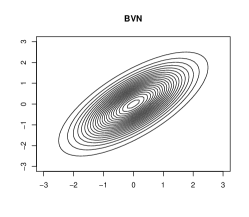
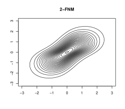
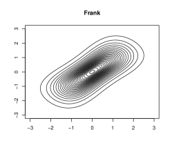
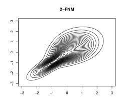
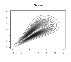
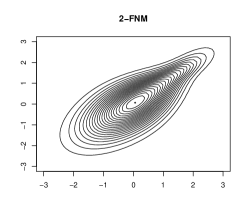
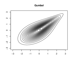
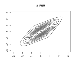
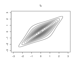
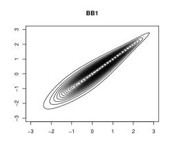
Figure 3 summarizes these results by depicting the contour plots of the 2- or 3-FNM copula with the parameters in Tables 1–3, i.e., the ones that the FNM copulas are close in terms of KL distance to the true copulas, and normal margins, along with the contour plots of the true copulas with normal margins. We summarize the case of $\tau=0.5$ ($\lambda_{L}=0.4,\lambda_{U}=0.6$ for BB1).

Table 3: Minimized KL distances and the corresponding 2-FNM or 3-FNM copula parameters and KL sample sizes for comparing the $t_{\nu}$ copula for a small $\nu$, with reflection symmetric tail dependence ($\lambda_{L}=\lambda_{U}$) as the Kendall’s $\tau$ varies from 0.1 to 0.9, versus the bivariate 2- or 3-FNM copula.

$\nu$	$\tau$	$\lambda_{L}$	$\lambda_{U}$	$K$	$\mbox{KL}(c_{1},c_{2})$	$\pi_{1}$	$\pi_{2}$	$\theta_{1}$	$\theta_{2}$	$\rho_{1}$	$\rho_{2}$	$\rho_{3}$	$n_{c_{1},c_{2}}$
2	0.1	0.24	0.24	3	0.004	0.004	0.436	2.003	-0.986	0.756	-0.582	0.689	1602
	0.2	0.30	0.30	3	0.004	0.005	0.365	1.988	-0.978	0.738	-0.531	0.731	1535
	0.3	0.37	0.37	3	0.004	0.005	0.291	2.037	-1.004	0.737	-0.488	0.769	1338
	0.4	0.44	0.44	3	0.006	0.006	0.221	1.978	-0.972	0.732	-0.443	0.808	1002
	0.5	0.52	0.52	3	0.008	0.010	0.170	1.653	-0.807	0.705	-0.350	0.852	640
	0.6	0.61	0.61	3	0.012	0.010	0.166	1.906	-0.938	0.735	0.057	0.906	375
	0.7	0.71	0.71	3	0.014	0.011	0.156	2.015	-0.997	0.817	0.435	0.945	498
	0.8	0.80	0.80	3	0.026	0.000	0.108	1.666	-0.819	0.599	0.441	0.976	181
	0.9	0.90	0.90	2	0.085	0.007		0.694		0.990	0.989		109
3	0.1	0.16	0.16	3	0.001	0.003	0.411	2.103	-1.037	0.688	-0.498	0.589	10194
	0.2	0.22	0.22	3	0.001	0.004	0.331	2.118	-1.044	0.656	-0.441	0.643	6923
	0.3	0.29	0.29	3	0.002	0.004	0.264	2.137	-1.053	0.638	-0.363	0.703	3576
	0.4	0.37	0.37	3	0.003	0.005	0.213	2.318	-1.143	0.626	-0.234	0.766	1865
	0.5	0.45	0.45	3	0.005	0.005	0.185	6.257	-3.115	0.691	0.004	0.830	1050
	0.6	0.55	0.55	3	0.006	0.007	0.195	2.103	-1.038	0.697	0.365	0.892	966
	0.7	0.66	0.66	3	0.006	0.008	0.206	2.085	-1.035	0.801	0.650	0.940	983
	0.8	0.77	0.77	3	0.023	0.000	0.051	0.265	-0.290	0.302	0.279	0.966	174
	0.9	0.88	0.88	3	0.050	0.001	0.000	0.761	0.621	0.154	0.171	0.987	123
4	0.1	0.11	0.11	3	0.000	0.001	0.403	2.609	-1.302	-0.990	-0.432	0.543	34841
	0.2	0.17	0.17	3	0.000	0.003	0.315	2.372	-1.172	0.626	-0.369	0.593	119419
	0.3	0.23	0.23	3	0.001	0.003	0.247	2.683	-1.326	0.545	-0.276	0.662	15265
	0.4	0.31	0.31	3	0.002	0.005	0.213	2.858	-1.409	0.545	-0.085	0.739	4058
	0.5	0.40	0.40	3	0.003	0.005	0.222	2.609	-1.288	0.611	0.229	0.820	2052
	0.6	0.50	0.50	3	0.003	0.006	0.259	2.596	-1.287	0.675	0.531	0.890	1935
	0.7	0.61	0.61	3	0.002	0.007	0.266	1.981	-0.985	0.775	0.738	0.938	3018
	0.8	0.74	0.74	2	0.025	0.951		0.925		0.949	0.848		256
	0.9	0.87	0.87	2	0.024	0.946		0.984		0.987	0.959		255
5	0.1	0.08	0.08	3	0.000	0.001	0.470	2.725	-1.345	-0.990	-0.315	0.532	168891
	0.2	0.13	0.13	3	-0.001	0.002	0.297	4.390	-2.169	0.674	-0.323	0.556	10836
	0.3	0.18	0.18	3	0.000	0.004	0.250	4.863	-2.408	0.473	-0.178	0.639	97784
	0.4	0.26	0.26	3	0.001	0.004	0.228	2.778	-1.371	0.513	0.043	0.726	7140
	0.5	0.35	0.35	3	0.003	0.001	0.245	0.469	-0.231	0.392	0.339	0.818	1450
	0.6	0.46	0.46	3	0.001	0.005	0.293	2.113	-1.047	0.642	0.598	0.886	3961
	0.7	0.58	0.58	3	0.001	0.006	0.326	1.879	-0.934	0.752	0.783	0.938	12785
	0.8	0.71	0.71	2	0.016	0.038		0.860		0.896	0.949		392
	0.9	0.85	0.85	2	0.015	0.035		0.970		0.967	0.987		394

If two copula models are applied to discrete variables and have the same strength of dependence as given by the Kendall’s $\tau$, then the KL distance gets smaller. This is because the different asymptotic rates in the joint tails of the copula density do not affect rectangle probabilities for the log-likelihood with discrete response (Joe,, 2014). This means that a discretized $K$-FNM copula model will be close to any copula model for discrete data even for strong dependence.

$\tau=0.5\quad\pi_{1}=0.5\quad\theta_{1}=0.45\quad\rho_{1}=0.65\quad\rho_{2}=0.65$		$\tau=0.5\quad\pi_{1}=0.5\quad\theta_{1}=0.88\quad\rho_{1}=0.40\quad\rho_{2}=0.40$
$\tau=0.5\quad\pi_{1}=0.75\quad\theta_{1}=0.96\quad\rho_{1}=0.41\quad\rho_{2}=0.86$		$\tau=0.5\quad\pi_{1}=0.11\quad\theta_{1}=0.94\quad\rho_{1}=0.83\quad\rho_{2}=0.60$
$\tau=0.5\quad\pi_{1}=0.01\quad\pi_{2}=0.17\quad\theta_{1}=1.65$		$\lambda_{L}=0.4\quad\lambda_{U}=0.6\quad\tau=0.59\quad\pi_{1}=0.03\quad\pi_{2}=0.55$
$\theta_{2}=-0.81\quad\rho_{1}=0.71\quad\rho_{2}=-0.35\quad\rho_{3}=0.85$		$\theta_{1}=1.73\quad\theta_{3}=-0.86\quad\rho_{1}=0.58\quad\rho_{2}=0.69\quad\rho_{3}=0.89$

Figure 3: Contour plots of the 2- or 3-FNM copula with the parameters in Tables 1–3, i.e., the ones that the FNM copulas are close in terms of KL distance to the true copulas, and normal margins, along with the contour plots of the true copulas with normal margins.

To show that we use ordinal response variables, say $Y_{1},Y_{2}$ with regressions on a scalar covariate $x$, which is assumed to take $\mathcal{X}$ values equally spaced in $[-1,1]$. Let $Z$ be a latent variable with cdf $\mathcal{F}$, such that $Y=y$ if $\alpha_{y}+\beta x\leq Z\leq\alpha_{y+1}+\beta x,\,y=0,\ldots,\mathcal{Y}-1,$ where $\mathcal{Y}$ is the number of categories of $Y$ (without loss of generality, we assume $\alpha_{0}=-\infty$ and $\alpha_{\mathcal{Y}}=\infty$), and $\beta$ is the slope of $x$. From this definition, the ordinal response $Y_{j}$ is assumed to have probability mass function (pmf)

$$\mathbb{P}(Y_{j}=y|x)=\mathcal{G}(\alpha_{y+1}+\beta_{j}x)-\mathcal{G}(\alpha_{y}+\beta_{j}x),\quad y=0,\ldots,\mathcal{Y}-1,\quad j=1,2.$$

Note that $\mathcal{G}$ normal leads to the probit model and $\mathcal{G}$ logistic leads to the cumulative logit model for ordinal response. With copula families, the bivariate pmf (see e.g., Nikoloulopoulos and Karlis, 2010) can be obtained as

$$f(y_{1},y_{2}|x) = C\Bigl{(}\mathcal{G}(\alpha_{y_{1}+1}+\beta_{1}x),\mathcal{G}(\alpha_{y_{2}+1}+\beta_{2}x)\Bigr{)}-C\Bigl{(}\mathcal{G}(\alpha_{y_{1}}+\beta_{1}x),\mathcal{G}(\alpha_{y_{2}+1}+\beta_{2}x)\Bigr{)}-$$ (7)

$$C\Bigl{(}\mathcal{G}(\alpha_{y_{1}+1}+\beta_{1}x),G(\alpha_{y_{2}}+\beta_{2}x)\Bigr{)}+C\Bigl{(}\mathcal{G}(\alpha_{y_{1}}+\beta_{1}x),\mathcal{G}(\alpha_{y_{2}}+\beta_{2}x)\Bigr{)}.$$

Let $f$ and $g$ denote the bivariate pmfs defined as in (7) for the bivariate Clayton and $K$-FNM copula, respectively. Then the $\mbox{KL}(f,g)$ is

$$\mbox{KL}(f,g)={{\sum}}_{x\in\mathcal{X}}{{\sum}}_{x\in\mathcal{X}}{{\sum}}_{y_{1}=0}^{\mathcal{Y}-1}{{\sum}}_{y_{2}=0}^{\mathcal{Y}-1}\log\left[\frac{f(y_{1},y_{2}|x)}{g(y_{1},y_{2}|x)}\right]f(y_{1},y_{2}|x).$$

Table 4: Minimized KL distances, corresponding 2-FNM copula parameters and KL sample sizes for comparing the discretized Clayton copula model, as the Kendall’s $\tau$ varies from 0.1 to 0.9, versus the discretized bivariate 2-FNM copula model. We use a varying number $\mathcal{Y}$ of ordinal categories (equally weighted) from 2 to 5 and choose $\mathcal{X}=5$, $\beta_{1}=1$ and $\beta_{2}=0.7$.

$\tau$	$\lambda_{L}$	$\mathcal{Y}$	$10^{3}\times\mbox{KL}(f,g)$	$\pi_{1}$	$\theta_{1}$	$\rho_{1}$	$\rho_{2}$	$n_{fg}$
0.1	0.04	2	0.003	0.950	0.908	0.080	-0.143	1788690
0.2	0.25		0.007	0.885	0.890	0.150	-0.898	721543
0.3	0.45		0.010	0.817	0.972	0.216	-0.558	534811
0.4	0.59		0.015	0.744	0.989	0.289	0.187	353990
0.5	0.71		0.017	0.678	0.981	0.380	0.607	311204
0.6	0.79		0.006	0.609	0.987	0.486	0.822	838516
0.7	0.86		0.042	0.574	0.995	0.671	0.933	122823
0.8	0.92		0.091	0.559	0.992	0.854	0.981	55142
0.9	0.96		0.190	0.773	0.980	0.983	1.000	30454
0.1	0.04	3	0.051	0.943	0.760	0.075	-0.865	106069
0.2	0.25		0.139	0.884	0.863	0.145	-0.430	39171
0.3	0.45		0.247	0.816	0.905	0.213	0.056	22213
0.4	0.59		0.331	0.746	0.916	0.284	0.470	16706
0.5	0.71		0.248	0.674	0.944	0.358	0.720	22017
0.6	0.79		0.196	0.609	0.990	0.467	0.856	27265
0.7	0.86		0.503	0.555	1.022	0.625	0.938	9672
0.8	0.92		0.791	0.503	1.022	0.802	0.981	5770
0.9	0.96		0.690	0.554	1.018	0.959	1.000	8247
0.1	0.04	4	0.114	0.945	0.755	0.075	-0.608	47632
0.2	0.25		0.330	0.884	0.832	0.144	-0.218	16580
0.3	0.45		0.598	0.820	0.875	0.214	0.206	9236
0.4	0.59		0.774	0.754	0.905	0.286	0.545	7137
0.5	0.71		0.704	0.683	0.948	0.363	0.743	7673
0.6	0.79		0.775	0.611	0.993	0.464	0.859	6808
0.7	0.86		1.429	0.546	1.024	0.609	0.935	3410
0.8	0.92		2.070	0.486	1.028	0.781	0.980	2213
0.9	0.96		2.387	0.622	1.024	0.964	1.000	2833
0.1	0.04	5	0.175	0.946	0.748	0.075	-0.511	31010
0.2	0.25		0.525	0.886	0.817	0.144	-0.121	10462
0.3	0.45		0.956	0.823	0.861	0.214	0.280	5787
0.4	0.59		1.216	0.757	0.899	0.285	0.582	4518
0.5	0.71		1.186	0.687	0.948	0.362	0.757	4535
0.6	0.79		1.449	0.615	0.996	0.464	0.864	3616
0.7	0.86		2.583	0.549	1.027	0.606	0.936	1892
0.8	0.92		3.752	0.482	1.029	0.772	0.979	1229
0.9	0.96		3.729	0.490	1.020	0.941	1.000	1593

Table 4 shows the minimized KL distances, the corresponding 2-FNM copula parameters and KL sample sizes for comparing the discretized Clayton copula model, as the Kendall’s $\tau$ varies from 0.1 to 0.9, versus the discretized 2-FNM copula model. We show the comparison results versus the Clayton copula, as in Table 1 it was revealed that the Clayton copula is the 1-parameter copula family which is the most far apart from the 2-FNM copula for continuous responses. We used univariate ordinal regressions, but note that using ordinal probit regressions led to similar results.

The conclusions from the table and the other computations we have done for other copula families are:

• The $K$-FNM copula is close to any parametric bivariate family of copulas if two copulas models are applied to discrete variables.

• With discrete response variables, it takes larger sample sizes to distinguish the $K$-FNM copula (because tails of the copula densities would not be “observed”).

• The KL distances (sample sizes) get larger (smaller) with less discretization, i.e., as $\mathcal{Y}$ increases.

4 Simulations

To gauge the small sample efficiency of the ML estimation method in Section 2.4 to estimate the $K$-FNM copula parameters, we performed several simulation studies using $K$-FNM copula models with various parameter choices for $K=2,3$. We report here typical results from these experiments.

We randomly generated $B=10^{4}$ samples of size $n=100,300,500$ from the 2-and 3-FNM bivariate copulas with exponential margins and marginal parameters $\lambda_{1}=0.5$ and $\lambda_{2}=1$. We have transformed the simulated data to uniform random variables using their empirical distributions, i.e., we have approached estimation of the $K$-FNM copula parameters using the semi-parametric estimation (Genest et al.,, 1995). We have used as initial values the ones that resemble the independence copula.

Table 5 contains the copula parameter values, the bias, standard deviation (SD) and the root mean square errors (RMSE) of the ML estimates, along with the average of their theoretical SDs. The theoretical SD of the ML estimate is obtained via the gradients and the Hessian computed numerically during the maximization process. The conclusions from the table and the other computations we have done are that

• ML is highly efficient according to the simulated biases, SDs and RMSEs as the sample size increases.

• The SDs computed from the simulations are close to the asymptotic SDs as the sample size increases.

• For small samples the estimates of the mean parameters $(\theta_{1},\ldots,\theta_{K-1})$ have upward bias.

Table 5: Small sample of sizes $N=100,300,500$ simulations ($10^{4}$ replications) from the 2- and 3-FNM copula model with exponential margins and biases, root mean square errors (RMSEs) and standard deviations (SDs), along with the square root of the average theoretical variances $(\sqrt{V})$ for the MLEs.

$K=2$
	$n$	$\pi_{1}=0.3$	$\theta_{1}=0$	$\rho_{1}=0.8$	$\rho_{2}=-0.8$
Bias	100	0.001	0.017	0.001	-0.001
	300	-0.001	0.009	0.002	-0.001
	500	-0.001	0.005	0.001	-0.001
SD	100	0.074	0.170	0.090	0.048
	300	0.039	0.086	0.042	0.026
	500	0.030	0.066	0.032	0.020
$\sqrt{V}$	100	0.046	0.111	0.066	0.039
	300	0.026	0.058	0.037	0.022
	500	0.019	0.042	0.028	0.017
RMSE	100	0.074	0.171	0.090	0.048
	300	0.039	0.087	0.042	0.026
	500	0.030	0.066	0.032	0.020

$K=3$
	$n$	$\pi_{1}=0.2$	$\pi_{1}=0.3$	$\theta_{1}=0.5$	$\theta_{2}=0.5$	$\rho_{1}=0.8$	$\rho_{2}=-0.8$	$\rho_{3}=0.8$
Bias	100	-0.028	-0.018	0.704	0.258	-0.093	0.088	-0.069
	300	-0.002	-0.001	0.113	0.041	-0.009	0.006	-0.005
	500	-0.001	0.000	0.031	-0.001	0.000	0.000	0.001
SD	100	0.120	0.091	1.054	0.932	0.320	0.222	0.205
	300	0.061	0.042	0.438	0.360	0.088	0.066	0.056
	500	0.041	0.031	0.209	0.182	0.064	0.038	0.030
$\sqrt{V}$	100	0.028	0.034	0.290	0.324	0.252	0.116	0.061
	300	0.022	0.024	0.089	0.086	0.060	0.041	0.031
	500	0.019	0.019	0.064	0.063	0.037	0.031	0.023
RMSE	100	0.123	0.093	1.268	0.967	0.333	0.238	0.217
	300	0.061	0.042	0.453	0.363	0.089	0.066	0.057
	500	0.041	0.031	0.211	0.182	0.064	0.038	0.030

5 Empirical examples

In this section we illustrate the proposed methodology by analysing two real data examples with distinct dependence structures, the first in the area of astrophysics and the second in agriculture. In Section 5.1 we analyse the two aforementioned MAGIC variables with peculiar dependence that typical bivariate copulas fail to model, while in Section 5.2 we analyse three variables from the 1985 survey of nutritional habits commissioned by the United States Department of Agriculture that have strong reflection asymmetric dependence.

We estimate each marginal distribution non-parametrically by the empirical distribution function of $Y_{j}$, viz.

$$u_{ij}=F_{j}(y_{ij})=\frac{1}{n+1}\sum_{i=1}^{n}\mathbf{1}(Y_{ij}\leq y_{ij})=r_{ij}/(n+1),$$

where $r_{ij}$ denotes the rank of $y_{ij}$. Hence we allow the distribution of the continuous margins to be quite free and not restricted by parametric families. We use simple diagnostics to identify the suitable copula family. Although copula theory uses transforms to standard uniform margins, for diagnostics, we convert the original data to normal scores using the normal quantiles of their empirical distributions. With a bivariate normal scores plot (Nikoloulopoulos et al.,, 2012) one can check for deviations from the elliptical shape that would be expected with the BVN copula, and hence assess if tail asymmetry exists on the data.

Having discussed why more flexible dependencies are needed we proceed with the $K$-FNM copula models and construct a plausible $K$-FNM copula model, to capture any type of dependence. For a baseline comparison, we initially fit the typical copula families presented in Section 3.1. To make it easier to compare strengths of dependence, we convert the estimated copula parameters to Kendall’s $\tau$’s, lower tail dependence $\lambda_{L}$ and upper tail dependence $\lambda_{U}$ via the relations in Joe, (2014, Chapter 4). The estimated Kendall’s $\tau$ of the $K$-FNM copula, viz.

$$\hat{\tau}(Y_{1},Y_{2};\hat{\pi}_{1},\ldots,\hat{\pi}_{K-1},\hat{\theta}_{1},\ldots,\hat{\theta}_{K-1},\hat{\rho}_{1},\ldots,\hat{\rho}_{K})=\\ -1+4\int_{0}^{1}\int_{0}^{1}C(u_{1},u_{2};\hat{\pi}_{1},\ldots,\hat{\pi}_{K-1},\hat{\theta}_{1},\ldots,\hat{\theta}_{K-1},\hat{\rho}_{1},\ldots,\hat{\rho}_{K})dC(u_{1},u_{2};\hat{\pi}_{1},\ldots,\hat{\pi}_{K-1},\hat{\theta}_{1},\ldots,\hat{\theta}_{K-1},\hat{\rho}_{1},\ldots,\hat{\rho}_{K}),$$

has been calculated via adaptive bivariate integration over hypercubes (Narasimhan et al.,, 2018); $C(\cdot;\cdot)$ is the $K$-FNM copula cdf given in (3).

To find a copula model that provides a good fit we don’t use goodness-of-fit procedures (see e.g., Genest et al., 2009 and the references therein), but we rather adopt the Akaike’s information criterion (AIC). The goodness-of-fit procedures involve a global distance measure between the model-based and empirical distribution, hence they might not be sensitive to tail behaviours and are not diagnostic in the sense of suggesting improved parametric models in the case of small $p$-values (Joe,, 2014). For vine copulas, Dissmann et al., (2013) found that pair-copula selection based on likelihood and AIC seem to be better than using bivariate goodness-of-fit tests. The AIC is

$$-2\times\ell+2\times\mbox{(\# model parameters) }$$

and a smaller AIC value indicates a copula model better approximates both the dependence structure of the data, and the strength of dependence in the tails.

5.1 MAGIC telescope

Ground-based atmospheric Cherenkov telescopes using the imaging technique are a useful addition to the variety of instruments used by astrophysicists. The MAGIC telescope, located on the Canary islands, observes high-energy gamma rays, detecting the radiation emitted by charged particles produced inside electromagnetic showers. Depending on the energy of the primary gamma, Cherenkov photons get collected, in patterns (called the shower image), allowing to discriminate statistically those caused by primary gammas (signal) from the images of hadronic showers initiated by cosmic rays in the upper atmosphere (background). Typically, the image of a shower is an elongated cluster; its long axis is oriented towards the camera center if the shower axis is parallel to the telescope’s optical axis, i.e. if the telescope axis is directed towards a point source. If the depositions were distributed as a BVN, this would be an equidensity ellipse. The characteristic parameters of this ellipse are among the image parameters. The energy depositions are typically asymmetric along the major axis (Bock et al.,, 2004).

We apply the $K$-FNM copula to 2 out of 10 MAGIC image parameters in Bock et al., (2004). Our objective is to describe the joint distribution of the Length and M3Long that have a peculiar dependence. The data set with the 10 MAGIC image parameters is available from the UCI Machine Learning Repository web page and comprises $n=19,020$ observations. In Figure 4 we depict the bivariate normal scores plot for the Length and M3Long. From the plot, it is revealed that none of the existing parametric families of copulas can adequately model the dependence structure between the variables.

Figure 4: Bivariate normal scores plot for the Length and M3Long variables.

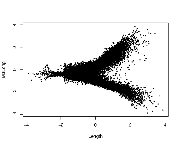
Table 6 gives the AICs, estimated copula parameters and their SE, along with the family-based Kendall’s $\tau$ and tail dependence parameters $\lambda_{L},\lambda_{U}$ for each fitted parametric family of copulas. The AICs show, that among the existing parametric families of copulas, the $t_{\delta}$ copula provides the best fit.

Table 6: AICs, estimated copula parameters and their standard errors (SE), along with the model-based Kendall’s $\tau$ and tail dependence parameters $\lambda_{L},\lambda_{U}$ for each fitted parametric family of copulas for the Length and M3Long variables.

Copula	AIC	$\theta$	SE	$\delta$	SE	$\tau$	$\lambda_{L}$	$\lambda_{U}$
BVN	-648.1	0.183	0.007			0.117
$t_{\delta}$	-4590.3	0.352	0.008	2.159	0.042	0.229	0.302	0.302
Clayton	2.1	0.000	0.002			0.000	0.000
Gumbel	-3069.4	1.314	0.007			0.239		0.305
Frank	-2004.5	2.167	0.049			0.230
BB1	-3059.3	0.001		1.314	0.007	0.239		0.305
BB7	-4110.6	1.591	0.013	0.001	0.021	0.249		0.454
Survival Clayton	-3363.7	0.651	0.013			0.246		0.345
Survival Gumbel	-228.1	1.102	0.007			0.093	0.125
Survival BB1	-3353.45	0.650	0.022	1.001	0.012	0.246	0.001	0.500
Survival BB7	-3355.2	1.001	0.013	0.651	0.014	0.246	0.001	0.345

Table 7: AICs, estimated $K$-FNM copula parameters and their standard errors (SE), along with the family-based Kendall’s $\tau$ for different number of components $K$ for the Length and M3Long variables.

		$K=2$			$K=3$
		Est.	SE		Est.	SE
$\pi_{1}$		0.127	0.001		0.001	0.000
$\pi_{2}$					0.334	0.000
$\theta_{1}$		-1.882	0.016		-1.045	0.002
$\theta_{2}$					-1.145	0.001
$\rho_{1}$		-0.784	0.006		-0.470	0.103
$\rho_{2}$		0.747	0.003		-0.854	0.003
$\rho_{3}$					0.901	0.001
$\tau$		0.304			0.310
AIC		-17320.5			-27064.1

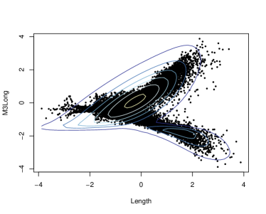
Then we exploit the use of the $K$-FNM copula to construct a plausible copula family to represent the joint distribution of Length and M3Long. Table 7 gives the AICs, estimated copula parameters and their SE, along with the family-based Kendall’s $\tau$ for different numbers of components. The AICs show, that the 3-FNM copula provides the best fit and provides much better fit than the $t_{\delta}$, since the AIC has been improved by $22473.8=-4590.3-(-27064.1)$. Note in passing that using $K>3$, the estimated mixing probabilities for the extra components were close to zero, and, hence, there was no improvement in fit. In Figure 5 we depict the estimated contour plots of the 2- and 3-FNM copulas with standard normal margins, along with the bivariate normal scores plots. From the plots, it is revealed that the 3-FNM copula provides a realistic representation of the joint distribution.

Figure 5: Estimated contour plots of the 2- and 3-FNM copulas with standard normal margins, along with the bivariate normal scores plot for the Length and M3Long variables.

$K=2$	$K=3$

The new-parametric family of copulas does not only allow to make accurate inferences that are based on the joint distribution, but also provides superior statistical inference for the parameters of interest, such as Kendall’s $\tau$. From Table 9, it is revealed that the Kendall’s $\tau$ was underestimated using simple parametric families of copulas and a change from a $\tau$-value of 0.23 ($t_{\delta}$-based) to one slightly larger than 0.30 has been achieved.

5.2 Nutritional habits

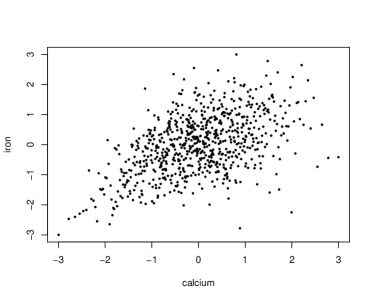
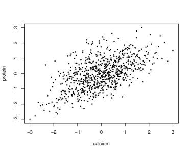
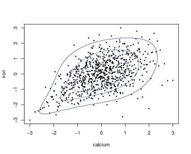
McNeil and Nešlehová, (2010) analysed three variables, namely daily calcium intake (in mg), daily iron intake (in mg) and daily protein intake (in g), of $n$=747 female respondents aged between 25 and 50 years to the 1985 survey of nutritional habits commissioned by the United States Department of Agriculture. This dataset and its description can be found in the R package lcopula (Belzile et al.,, 2019). Genest et al., (2012) identified a strongly asymmetric dependence structure between the intakes of calcium and iron, and between the intakes of calcium and protein. In this section we apply the $K$-FNM copula to the pairs identified as asymmetric to illustrate that it can sufficiently allow for reflection asymmetric dependence. In Figure 6 we depict the bivariate normal scores plots for the pairs identified as asymmetric. From the plots, it is revealed that there is more skewness in the lower tail.

Figure 6: Bivariate normal scores plots for the pairs identified as asymmetric in the nutrient data set.

Table 8: AICs, estimated copula parameters and their standard errors (SE), along with the model-based Kendall’s $\tau$ and tail dependence parameters $\lambda_{L},\lambda_{U}$ for each fitted parametric family of copulas for the pairs identified as asymmetric in the nutrient data set.

Calcium and Iron
Copula	AIC	$\hat{\theta}$	SE	$\hat{\delta}$	SE	$\hat{\tau}$	$\hat{\lambda}_{L}$	$\hat{\lambda}_{U}$
BVN	-203.0	0.497	0.025			0.331
$t_{\delta}$	-216.6	0.492	0.030	6.563	2.026	0.328	0.149	0.149
Clayton	-230.7	0.885	0.069			0.307	0.457
Gumbel	-162.0	1.412	0.040			0.292		0.366
Frank	-173.0	3.140	0.238			0.319
BB1	-238.3	0.684	0.091	1.115	0.043	0.332	0.403	0.138
BB7	-238.9	1.165	0.059	0.807	0.075	0.329	0.424	0.187
Survival Clayton	-114.8	0.582	0.061			0.225		0.304
Survival Gumbel	-239.6	1.490	0.043			0.329	0.408
Survival BB1	-237.7	0.016	0.063	1.480	0.057	0.330	0.403	0.626
Survival BB7	-240.6	1.611	0.069	0.270	0.070	0.320	0.462	0.077
Calcium and Protein
Copula	AIC	$\hat{\theta}$	SE	$\hat{\delta}$	SE	$\hat{\tau}$	$\hat{\lambda}_{L}$	$\hat{\lambda}_{U}$
BVN	-267.8	0.558	0.022			0.377
$t_{\delta}$	-268.9	0.553	0.025	12.323	6.752	0.373	0.072	0.072
Clayton	-261.7	0.965	0.071			0.325	0.487
Gumbel	-217.2	1.499	0.043			0.333		0.412
Frank	-227.2	3.657	0.244			0.362
BB1	-282.3	0.633	0.091	1.196	0.049	0.365	0.401	0.215
BB7	-281.3	1.264	0.066	0.838	0.079	0.357	0.437	0.270
Survival Clayton	-166.0	0.714	0.064			0.263		0.379
Survival Gumbel	-283.3	1.567	0.045			0.362	0.444
Survival BB1	-284.4	0.115	0.068	1.493	0.060	0.367	0.409	0.629
Survival BB7	-284.6	1.632	0.073	0.407	0.074	0.354	0.471	0.182

Table 8 gives the AICs, estimated copula parameters and their SE, along with the family-based Kendall’s $\tau$ and tail dependence parameters $\lambda_{L},\lambda_{U}$ for each fitted parametric family of copulas. The AICs show, that among the existing parametric families of copulas, the survival BB7 copula provides the best fit for both pairs identified as asymmetric.

Table 9: AICs and estimated $2$-FNM copula parameters along with their standard errors (SE) for the pairs identified as asymmetric in the nutrient data set.

		Calcium and Iron			Calcium and Protein
		Est.	SE		Est.	SE
$\pi$		0.848	0.055		0.953	0.008
$\theta$		0.518	0.136		2.012	0.094
$\rho_{1}$		0.339	0.044		0.474	0.030
$\rho_{2}$		0.779	0.062		0.594	0.108
$\tau$		0.330			0.341
AIC		-243.7			-291.7

Figure 7: estimated contour plots of the 2-FNM and survival BB7 copulas with standard normal margins, along with the bivariate normal scores plot for the pairs identified as asymmetric in the nutrient data set.

2-FNM	Survival BB7
2-FNM	Survival BB7

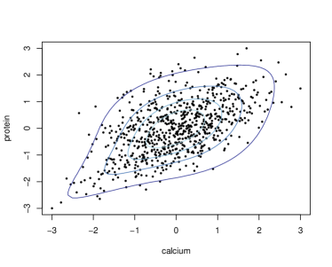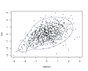
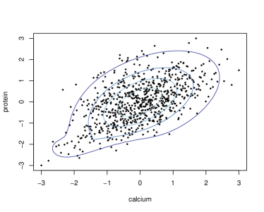
Then we exploit the use of the $K$-FNM copula to construct a plausible copula family to represent the joint distribution of both pairs of variables. It has been revealed, that for both pairs $K=2$ mixture components are sufficient to describe their dependence. Table 9 gives the AICs and estimated 2-FNM copula parameters, along with their standard errors. The AICs show, that between the intakes of calcium and iron and between the intakes of calcium and protein the 2-FNM copula provides better fit than the survival BB7, since the AIC has been improved by $3.1=-240.6-(-243.7)$ and $7.1=-284.6-(-291.7)$, respectively. In Figure 7 we depict the estimated contour plots of the 2-FNM and survival BB7 copulas with standard normal margins, along with the bivariate normal scores plot for the pairs identified as asymmetric in the nutrient data set. From the plots, it is revealed that the 2-FNM copula provides a nearly identical or even better representation of the joint distribution compared to the survival BB7 (best fit amongst the existing parametric families of copulas).

6 Discussion

We have proposed the $K$-FNM parametric family of bivariate copulas and demonstrated that the new family is so flexible, it removes the ad-hoc constraints on the tails of existing parametric copula families, and is able to handle various dependence patterns that appear in the existing parametric bivariate copula families.

There exist many bivariate copula families, and as the new copula family can “nearly” approximate any of these, the selection of the appropriate copula family among many candidates can be subsided by solely using the $K$-FNM copula. This applies when the data are continuous and have weak to moderate dependence and when the data are discrete for any different strength of dependence.

Given that bivariate copulas are building blocks for many multivariate dependence models such as the vine (e.g., Nikoloulopoulos et al., 2012; Panagiotelis et al., 2012; Dissmann et al., 2013) and factor (e.g., Krupskii and Joe, 2013; Nikoloulopoulos and Joe, 2015; Kadhem and Nikoloulopoulos, 2021) copula models, there is much potential of the proposed copula for building up more complex multivariate dependence models. Future research will focus on exploring this potential in modelling real multivariate datasets that have complex dependence structures.

References

- Belzile et al., (2019) Belzile, L., Genest, C., McNeil, A. J., and Nešlehová, J. G. (2019). lcopula: Liouville Copulas. R package version 1.0.4. URL: http://CRAN.R-project.org/package=lcopula.
- Bock et al., (2004) Bock, R., Chilingarian, A., Gaug, M., Hakl, F., Hengstebeck, T., Jiřina, M., Klaschka, J., Kotrč, E., Savický, P., Towers, S., Vaiciulis, A., and Wittek, W. (2004). Methods for multidimensional event classification: a case study using images from a cherenkov gamma-ray telescope. Nuclear Instruments and Methods in Physics Research Section A: Accelerators, Spectrometers, Detectors and Associated Equipment, 516(2):511–528.
- Czado, (2019) Czado, C. (2019). Analyzing dependent data with vine copulas, volume 222 of Lecture Notes in Statistics. Springer.
- Dalla Valle et al., (2018) Dalla Valle, L., Leisen, F., and Rossini, L. (2018). Bayesian non-parametric conditional copula estimation of twin data. Journal of the Royal Statistical Society: Series C (Applied Statistics), 67(3):523–548.
- Dissmann et al., (2013) Dissmann, J., Brechmann, E., Czado, C., and Kurowicka, D. (2013). Selecting and estimating regular vine copulae and application to financial returns. Computational Statistics & Data Analysis, 59:52–69.
- Durrleman et al., (2000) Durrleman, V., Nikeghbali, A., and Roncalli, T. (2000). Which copula is the right one? Technical Report, Groupe de Researche Operationnelle Credit-Lyonnais.
- Genest et al., (1995) Genest, C., Ghoudi, K., and Rivest, L.-P. (1995). A semiparametric estimation procedure of dependence parameters in multivariate families of distributions. Biometrika, 82(3):543–552.
- Genest et al., (2012) Genest, C., Nešlehová, J., and Quessy, J.-F. (2012). Tests of symmetry for bivariate copulas. Annals of the Institute of Statistical Mathematics, 64(4):811–834.
- Genest et al., (2009) Genest, C., Rémillard, B., and Beaudoin, D. (2009). Goodness-of-fit tests for copulas: A review and a power study. Insurance: Mathematics & Economics, 44:199–213.
- Hua and Joe, (2011) Hua, L. and Joe, H. (2011). Tail order and intermediate tail dependence of multivariate copulas. Journal of Multivariate Analysis, 102(10):1454–1471.
- Huard et al., (2006) Huard, D., Évin, G., and Favre, A.-C. (2006). Bayesian copula selection. Computational Statistics & Data Analysis, 51(2):809–822.
- Joe, (1993) Joe, H. (1993). Parametric families of multivariate distributions with given margins. Journal of Multivariate Analysis, 46:262–282.
- Joe, (1997) Joe, H. (1997). Multivariate Models and Dependence Concepts. Chapman & Hall, London.
- Joe, (2005) Joe, H. (2005). Asymptotic efficiency of the two-stage estimation method for copula-based models. Journal of Multivariate Analysis, 94(2):401–419.
- Joe, (2014) Joe, H. (2014). Dependence Modeling with Copulas. Chapman & Hall, London.
- Joe et al., (2010) Joe, H., Li, H., and Nikoloulopoulos, A. K. (2010). Tail dependence functions and vine copulas. Journal of Multivariate Analysis, 101:252–270.
- Kadhem and Nikoloulopoulos, (2021) Kadhem, S. H. and Nikoloulopoulos, A. K. (2021). Factor copula models for mixed data. British Journal of Mathematical and Statistical Psychology. DOI: 10.1111/bmsp.12231.
- Krupskii and Joe, (2013) Krupskii, P. and Joe, H. (2013). Factor copula models for multivariate data. Journal of Multivariate Analysis, 120:85–101.
- McNeil and Nešlehová, (2010) McNeil, A. J. and Nešlehová, J. (2010). From Archimedean to Liouville copulas. Journal of Multivariate Analysis, 101(8):1772–1790.
- Nagler and Czado, (2016) Nagler, T. and Czado, C. (2016). Evading the curse of dimensionality in nonparametric density estimation with simplified vine copulas. Journal of Multivariate Analysis, 151:69–89.
- Narasimhan et al., (2018) Narasimhan, B., Koller, M., Johnson, S. G., Hahn, T., Bouvier, A., Kiêu, K., and Gaure, S. (2018). cubature: Adaptive multivariate integration over hypercubes. R package version 2.0.3. URL: http://CRAN.R-project.org/package=cubature.
- Nash, (1990) Nash, J. (1990). Compact Numerical Methods for Computers: Linear Algebra and Function Minimisation. Hilger, New York. 2nd edition.
- Nelsen, (2006) Nelsen, R. B. (2006). An Introduction to Copulas. Springer-Verlag, New York.
- Nikoloulopoulos, (2013) Nikoloulopoulos, A. K. (2013). Copula-based models for multivariate discrete response data. In Durante, F., Härdle, W., and Jaworski, P., editors, Copulae in Mathematical and Quantitative Finance, volume vol 213, pages 231–249, Berlin, Heidelberg. Springer.
- Nikoloulopoulos, (2015) Nikoloulopoulos, A. K. (2015). A mixed effect model for bivariate meta-analysis of diagnostic test accuracy studies using a copula representation of the random effects distribution. Statistics in Medicine, 34:3842–3865.
- Nikoloulopoulos and Joe, (2015) Nikoloulopoulos, A. K. and Joe, H. (2015). Factor copula models for item response data. Psychometrika, 80:126–150.
- Nikoloulopoulos et al., (2012) Nikoloulopoulos, A. K., Joe, H., and Li, H. (2012). Vine copulas with asymmetric tail dependence and applications to financial return data. Computational Statistics & Data Analysis, 56:659–3673.
- Nikoloulopoulos and Karlis, (2008) Nikoloulopoulos, A. K. and Karlis, D. (2008). Copula model evaluation based on parametric bootstrap. Computational Statistics & Data Analysis, 52:3342–3353.
- Nikoloulopoulos and Karlis, (2009) Nikoloulopoulos, A. K. and Karlis, D. (2009). Finite normal mixture copulas for multivariate discrete data modeling. Journal of Statistical Planning and Inference, 139:3878–3890.
- Nikoloulopoulos and Karlis, (2010) Nikoloulopoulos, A. K. and Karlis, D. (2010). Regression in a copula model for bivariate count data. Journal of Applied Statistics, 37:1555–1568.
- Panagiotelis et al., (2012) Panagiotelis, A., Czado, C., and Joe, H. (2012). Pair copula constructions for multivariate discrete data. Journal of the American Statistical Association, 107:1063–1072.
- Sklar, (1959) Sklar, M. (1959). Fonctions de répartition à dimensions et leurs marges. Publications de l’Institut de Statistique de l’Université de Paris, 8:229–231.
- Stroud and Secrest, (1966) Stroud, A. H. and Secrest, D. (1966). Gaussian Quadrature Formulas. Prentice-Hall, Englewood Cliffs, NJ.
- Wu et al., (2015) Wu, J., Wang, X., and Walker, S. G. (2015). Bayesian nonparametric estimation of a copula. Journal of Statistical Computation and Simulation, 85(1):103–116.