Periodic thermodynamics of the parametrically driven harmonic oscillator

Abstract

We determine the quasistationary distribution of Floquet-state occupation probabilities for a parametrically driven harmonic oscillator coupled to a thermal bath. Since the system exhibits detailed balance, and the canonical representatives of its quasienergies are equidistant, these probabilities are given by a geometrical Boltzmann distribution, but its quasitemperature differs from the actual temperature of the bath, being affected by the functional form of the latter’s spectral density. We provide two examples of quasithermal engineering, i.e., of deliberate manipulation of the quasistationary distribution by suitable design of the spectral density: We show that the driven system can effectively be made colder than the undriven one, and demonstrate that quasithermal instability can occur even when the system is mechanically stable.

I Introduction

If a quantum system governed by a time-independent Hamiltonian possessing eigenstates with energies $E_{n}$ is coupled to a thermal reservoir having the temperature $T_{\rm bath}$, and is given time to equilibrate, after a while each state will be populated with probability proportional to its respective Boltzmann factor $\exp(-\beta E_{n})$, where $\beta=1/(k_{\rm B}T_{\rm bath})$, with $k_{\rm B}$ denoting the Boltzmann constant LandauLifshitzV ; Reif09 ; Pathria11 . If a time-periodically driven quantum system possessing Floquet states with quasienergies $\varepsilon_{n}$ is coupled to such a reservoir it will likewise approach a quasistationary state characterized by certain occupation probabilities $p_{n}$ of its Floquet states, but such distributions of Floquet-state occupation probabilities are lacking the universality of their equilibrium counterpart. The determination of such distributions is a major task of what may be termed periodic thermodynamics, as it has been formulated in a programmatic manner by Kohn Kohn01 , and approached constructively by Breuer et al. BreuerEtAl00 So far, knowledge about such quasistationary Floquet-state distributions is quite limited, although some statements have been derived for special classes of systems ShiraiEtAl15 ; Liu15 . Remarkably, a linearly driven harmonic oscillator interacting with a harmonic-oscillator heat bath retains the Boltzmann distribution of the bath, that is, the Floquet states of the linearly driven harmonic oscillator are occupied according to a Boltzmann distribution with the bath temperature BreuerEtAl00 ; LangemeyerHolthaus14 . On the other hand, the Floquet substates of a spin $s$ exposed to a circularly polarized driving force while being coupled to a heat bath develop a Boltzmann distribution with an effective quasitemperature which differs from the actual temperature of the bath SchmidtEtAl19 . In the case of strongly driven anharmonic oscillators the quasistationary Floquet-state distributions can be significantly influenced by phase-space structures of the corresponding classical system BreuerEtAl00 ; KetzmerickWustmann10 . Intriguingly, the quasistationary distributions of driven-dissipative ideal Bose gases allow for Bose-Einstein condensation into multiple states VorbergEtAl13 ; SchnellEtAl18 . These somewhat random snapshots indicate that the subject of quasistationary Floquet-state distributions merits systematic further investigation.

In the present work we explore the periodic thermodynamics of a model system which is substantially richer than the linearly driven harmonic oscillator but still retains much of its analytical simplicity, namely, the harmonic oscillator with a periodically time-dependent spring function. The parametrically driven harmonic oscillator with an arbitrary time-dependence of its spring function has been the subject of several seminal studies, among others by Husimi Husimi53 , Lewis and Riesenfeld LewisRiesenfeld69 , and by Popov and Perelomov PopovPerelomov69 , on the grounds of which it is a relatively straightforward exercise to derive the Floquet states which emerge when the spring function depends on time in a periodic manner PopovPerelomov70 ; Combescure86 ; Brown91 . Nonetheless, we will sketch the construction of the Floquet states in some detail in Sec. II below, as the precise knowledge of these states is necessary for specifying their coupling to the bath, and for computing the bath-induced transition rates. In Sec. III we will then provide typical numerical examples for the variation of the system’s quasienergies with the driving strength, focusing on the archetypal case for which the classical equation of motion reduces to the well-known Mathieu equation. The central Sec. IV outlines the calculation of corresponding quasistationary distributions; this calculation is greatly facilitated by the fact that the system exhibits detailed balance. We also consider the energy dissipation rate pertaining to the nonequilibrium steady state for various spectral densities of the bath. One of the noteworthy benefits of this elemental model of periodic thermodynamics lies in the fact that it also provides a particularly transparent, analytical access to the question how the quasistationary distribution is affected if the spectral density is modified or, phrased the other way round, how the spectral density has to be designed in order to obtain quasistationary distributions with certain desired properties; this option of quasithermal engineering is discussed in the concluding Sec. V.

II Floquet states of the parametrically driven harmonic oscillator

Consider a quantum particle of mass $M$ moving in a one-dimensional harmonic-oscillator potential with time-dependent spring function $k(t)$, as described in the position representation by the Hamiltonian

$$H_{0}(t)=\frac{p^{2}}{2M}+\frac{1}{2}k(t)x^{2}\;.$$ (1)

Later on we will focus on spring functions which depend periodically on time $t$, but at this point we still admit an arbitrary variation of $k$ with $t$, requiring only the existence of the solutions to the corresponding classical equations of motion; the significance of this requirement will soon become obvious. For solving the time-dependent Schrödinger equation

$$\left(H_{0}(t)-{\mathrm{i}}\hbar\frac{\partial}{\partial t}\right)\psi(x,t)=0$$ (2)

we follow a strategy devised by Brown Brown91 , and apply a sequence of two unitary transformations to Eq. (2) which bring the Hamiltonian (1) into a more convenient form. Intending to replace the time-dependent potential $k(t)x^{2}/2$ by a more tractable one, we perform a first transformation which is implemented by Brown91

$$U_{1}=\exp\big{(}-{\mathrm{i}}\eta(t)x^{2}/\hbar\big{)}\;,$$ (3)

where the function $\eta(t)$ will be suitably specified below. Using the familiar Lie expansion formula Miller72

$${\mathrm{e}}^{A}B{\mathrm{e}}^{-A} = B+[A,B]+\frac{1}{2}\Big{[}A,[A,B]\Big{]}+\ldots$$ (4)

$$+\frac{1}{n!}\Big{[}A,\ldots[A,B]\Big{]}_{(n)}+\ldots$$

for operators $A$ and $B$, which reduces to

$${\mathrm{e}}^{A}B{\mathrm{e}}^{-A}=B+[A,B]$$ (5)

if $\big{[}A,[A,B]\big{]}=0$, one finds

$$U_{1}x\,U_{1}^{\dagger} = x$$

$$U_{1}p\,U_{1}^{\dagger} = p+2\eta(t)x$$

$$U_{1}\big{(}-{\mathrm{i}}\hbar\partial/\partial t\big{)}U_{1}^{\dagger} = -{\mathrm{i}}\hbar\partial/\partial t+\dot{\eta}(t)x^{2}\;.$$ (6)

Taken together, these relations yield

$$U_{1}\left(\frac{p^{2}}{2M}+\frac{1}{2}k(t)x^{2}-{\mathrm{i}}\hbar\frac{\partial}{\partial t}\right)U_{1}^{\dagger}$$ (7)

$$= \frac{p^{2}}{2M}+\left[\frac{2}{M}\eta^{2}(t)+\frac{1}{2}k(t)+\dot{\eta}(t)\right]x^{2}-{\mathrm{i}}\hbar\frac{\partial}{\partial t}$$

$$+ \frac{\eta(t)}{M}\big{(}px+xp\big{)}\;.$$

For constructing the required counterterm to the coefficient $k(t)/2$ of $x^{2}$ appearing in the square brackets here, we resort to a solution $\xi(t)\equiv\xi$ to the classical equation of motion

$$M\ddot{\xi}+k(t)\xi=0\;;$$ (8)

for ease of notation, the time-dependence of $\xi$ will not be indicated explicitly. If we demand that $\xi$ be complex, its conjugate $\xi^{*}$ is a second, linearly independent solution to Eq. (8). It is easy to show that the Wronskian of these two solutions is time-independent, and purely imaginary, so that we may write

$$\left|\begin{array}[]{cc}\dot{\xi}&\dot{\xi}^{*}\\ \xi&\xi^{*}\end{array}\right|=2{\mathrm{i}}\Omega\;,$$ (9)

where

$$\Omega={\rm Im}(\dot{\xi}\xi^{*})\;;$$ (10)

without loss of generality (that is, interchanging $\xi$ and $\xi^{*}$ if necessary), we may stipulate $\Omega>0$. Given these classical solutions $\xi$ and $\xi^{*}$, we now set Brown91

$$\eta(t)=\frac{M}{4}\left(\frac{\dot{\xi}}{\xi}+\frac{\dot{\xi}^{*}}{\xi^{*}}\right)=\frac{M}{4}\frac{{\mathrm{d}}}{{\mathrm{d}}t}\ln|\xi|^{2}\;,$$ (11)

providing

$$\dot{\eta}(t) = \frac{M}{4}\left(\frac{\ddot{\xi}}{\xi}-\frac{\dot{\xi}^{2}}{\xi^{2}}+\frac{\ddot{\xi}^{*}}{\xi^{*}}-\frac{\dot{\xi}^{*2}}{\xi^{*2}}\right)$$ (12)

$$= \frac{M}{4}\left(-\frac{2k(t)}{M}-\frac{\dot{\xi}^{2}\xi^{*2}+\dot{\xi}^{*2}\xi^{2}}{|\xi|^{4}}\right)\;.$$

This is how the counterterm comes into play, but in view of Eq. (7) we also need to account for a further contribution to the transformed quadratic potential, given by

$$\frac{2}{M}\eta^{2}(t)=\frac{M}{8}\frac{1}{|\xi|^{4}}\left(\dot{\xi}^{2}\xi^{*2}+2\xi\,\dot{\xi}\,\xi^{*}\,\dot{\xi}^{*}+\xi^{2}\dot{\xi}^{*2}\right)\;.$$ (13)

Adding up, and making use of the Wronskian (9), one finds

$$\frac{2}{M}\eta^{2}(t)+\frac{1}{2}k(t)+\dot{\eta}(t)=\frac{1}{2}M\Omega^{2}\frac{1}{|\xi|^{4}}\;.$$ (14)

At this point, it may be appropriate to point out that the construction still leaves us with some indeterminacy: The classical equation (8) is homogeneous, so that $\xi$ may be taken to be dimensionless, and we are free to multiply any solution $\xi$ by an arbitrary constant. Thus, $\Omega$ is not well defined, but $\Omega/|\xi|^{2}$ is. Note also that this multiplicative freedom does not affect the function $\eta(t)$, as a consequence of its definition (11), implying that the transformation (7) indeed is unique.

At a first glance, it seems that this transformation (7) with the particular choice (11) for the function $\eta(t)$ has not brought us any further. On the contrary: Effectively, the spring function $k(t)$ with its known time-dependence has been replaced by $M\Omega^{2}/|\xi|^{4}$, the time-dependence of which still needs to be determined by solving the classical Eq. (8). However, the actual progress achieved by the operation (3) stems from the last term on the right-hand side of Eq. (7). Namely, one evidently has

$$\left[\frac{{\mathrm{i}}}{\hbar}\frac{xp+px}{2},x\right] \;=\; \phantom{-}x$$

$$\left[\frac{{\mathrm{i}}}{\hbar}\frac{xp+px}{2},p\right] \;=\; -p\;,$$ (15)

so that the application of the transformation formula (4) to the unitary operator

$$S_{\lambda}=\exp\left(\frac{{\mathrm{i}}}{\hbar}\ln\lambda\frac{xp+px}{2}\right)$$ (16)

with arbitrary $\lambda>0$ results in both

$$S_{\lambda}x\,S_{\lambda}^{\dagger}\;=\;\sum_{n=0}^{\infty}\frac{(\ln\lambda)^{n}}{n!}x\;=\;\lambda x$$ (17)

and

$$S_{\lambda}p\,S_{\lambda}^{\dagger}\;=\;\sum_{n=0}^{\infty}\frac{(-\ln\lambda)^{n}}{n!}p\;=\;\frac{1}{\lambda}p\;.$$ (18)

Thus, $S_{\lambda}$ implements a scale transformation, leaving the product $px$ invariant. If we now admit a time-dependent scaling parameter $\lambda=\lambda(t)$, we also have

$$S_{\lambda(t)}\left(-{\mathrm{i}}\hbar\frac{\partial}{\partial t}\right)S_{\lambda(t)}^{\dagger}=-{\mathrm{i}}\hbar\frac{\partial}{\partial t}-\frac{\dot{\lambda}(t)}{\lambda(t)}\,\frac{xp+px}{2}\;.$$ (19)

Returning to Eq. (7), this allows us to achieve two goals simultaneously: Equating

$$\frac{\dot{\lambda}(t)}{\lambda(t)}=2\frac{\eta(t)}{M}\;,$$ (20)

which by Eq. (11) is equivalent to

$$\frac{{\mathrm{d}}}{{\mathrm{d}}t}\ln\lambda(t)=\frac{{\mathrm{d}}}{{\mathrm{d}}t}\ln|\xi|\;,$$ (21)

we may set

$$\lambda(t)=|\xi|$$ (22)

and define a second unitary transformation

$$U_{2}=S_{|\xi|}\;,$$ (23)

effectuating

$$U_{2}U_{1}\left(H_{0}(t)-{\mathrm{i}}\hbar\frac{\partial}{\partial t}\right)U_{1}^{\dagger}U_{2}^{\dagger}$$ (24)

$$= U_{2}\left(\frac{p^{2}}{2M}+\frac{1}{2}M\Omega^{2}\frac{x^{2}}{|\xi|^{4}}-{\mathrm{i}}\hbar\frac{\partial}{\partial t}+\frac{\eta(t)}{M}\big{(}px+xp\big{)}\right)U_{2}^{\dagger}$$

$$= \frac{1}{|\xi|^{2}}\left[\frac{p^{2}}{2M}+\frac{1}{2}M\Omega^{2}x^{2}\right]-{\mathrm{i}}\hbar\frac{\partial}{\partial t}\;.$$

Thus we have both scaled the momentum $p$ by $1/|\xi|$ and the position $x$ by $|\xi|$, allowing us to take a time-dependent factor $1/|\xi|^{2}$ out of the square brackets, and have removed the annoying last term that had appeared on the right-hand side of Eq. (7).

Observe also that there is a further unexploited freedom: Integration of Eq. (21) leaves us with an arbitrary constant $\ln c$, so that we might have chosen $\lambda(t)=c|\xi|$ instead of Eq. (22). This would have led to a renormalization of the mass in the last line of Eq. (24), shifting $M$ to $Mc^{2}$. As will become evident below, this freedom again has no observable consequences.

Now the result of the two-step transformation (24) prompts us to solve the modified Schrödinger equation

$${\mathrm{i}}\hbar\frac{\partial}{\partial t}\chi(x,t)=\frac{1}{|\xi|^{2}}H_{\rm osc}\chi(x,t)\;,$$ (25)

instead of Eq. (2), where

$$H_{\rm osc}=\frac{p^{2}}{2M}+\frac{1}{2}M\Omega^{2}x^{2}$$ (26)

is the Hamiltonian of a time-independent harmonic oscillator Husimi53 ; LewisRiesenfeld69 ; PopovPerelomov69 , possessing the eigenfunctions

$$\chi_{n}^{\rm osc}(x)=\frac{\pi^{-1/4}}{\sqrt{2^{n}n!\,L}}\,H_{n}(x/L)\,\exp\!\big{(}-(x/L)^{2}/2\big{)}$$ (27)

with integer quantum numbers $n=0,1,2,\ldots$, Hermite polynomials $H_{n}$, and oscillator length $L=\sqrt{\hbar/(M\Omega)}$, yielding the energy eigenvalues $E_{n}=\hbar\Omega(n+1/2)$. Inserting the natural ansatz

$$\chi_{n}(x,t)=\exp\!\big{(}-{\mathrm{i}}\gamma_{n}(t)/\hbar\big{)}\,\chi_{n}^{\rm osc}(x)$$ (28)

into Eq. (25), one finds

$$\dot{\gamma}_{n}(t)=\frac{1}{|\xi|^{2}}E_{n}\;.$$ (29)

This equation for the desired phase $\gamma_{n}(t)$ can be brought into a more transparent form: Introducing the phase $\varphi(t)$ of the complex trajectory $\xi$ according to

$$\xi=|\xi|\exp\!\big{(}{\mathrm{i}}\varphi(t)\big{)}$$ (30)

or

$$\frac{\xi}{\xi^{*}}=\exp\!\big{(}2{\mathrm{i}}\varphi(t)\big{)}\;,$$ (31)

one derives

$$\frac{{\mathrm{d}}}{{\mathrm{d}}t}\frac{\xi}{\xi^{*}}=\frac{\dot{\xi}\xi^{*}-\xi\dot{\xi}^{*}}{\xi^{*2}}=2{\mathrm{i}}\dot{\varphi}(t)\,\exp\!\big{(}2{\mathrm{i}}\varphi(t)\big{)}\;.$$ (32)

Again invoking the Wronskian (9), this becomes

$$\dot{\varphi}(t)=\frac{\Omega}{|\xi|^{2}}\;;$$ (33)

recall that this expression is not affected by the freedom to scale $\xi$ by an arbitrary factor. Hence, Eq. (29) takes the form

$$\dot{\gamma}_{n}(t)=\frac{E_{n}}{\Omega}\dot{\varphi}(t)\;;$$ (34)

observe that the frequency $\Omega$ of the auxiliary oscillator (26) drops out here. Integrating, we have fully determined the solutions (28) to Eq. (25):

$$\chi_{n}(x,t)=\exp\!\Big{(}-{\mathrm{i}}(n+1/2)\big{[}\varphi(t)-\varphi(0)\big{]}\Big{)}\chi_{n}^{\rm osc}(x)\;,$$ (35)

having stipulated $\gamma(0)=0$. The appearance of $\varphi(0)$ makes sure that these solutions (35) remain invariant under a constant shift of the phase of $\xi$, as does the effective Hamiltonian $H_{\rm osc}/|\xi|^{2}$.

Next, we need to invert the two transformations (23) and (3) in order to obtain the solutions of the original Schrödinger equation (2). Utilizing the identity

$$S_{\lambda}f(x)=\sqrt{\lambda}f(\lambda x)\;,$$ (36)

which may be verified by differentiating both sides with respect to $\lambda$, one finds

$$\psi_{n}(x,t) = U_{1}^{\dagger}U_{2}^{\dagger}\,\chi_{n}(x,t)$$

$$= \exp\!\Big{(}-{\mathrm{i}}(n+1/2)\big{[}\varphi(t)-\varphi(0)\big{]}\Big{)}u_{n}^{\rm osc}(x,t)\;,$$

where

$$u_{n}^{\rm osc}(x,t)=\exp\!\left(\frac{{\mathrm{i}}M}{2\hbar}x^{2}\frac{{\mathrm{d}}}{{\mathrm{d}}t}\ln|\xi|\right)\frac{1}{\sqrt{|\xi|}}\chi_{n}^{\rm osc}\!\left(\frac{x}{|\xi|}\right)\;;$$ (38)

of course, this expression agrees with the known solutions obtained by other approaches Husimi53 ; LewisRiesenfeld69 ; PopovPerelomov69 . Had we utilized the freedom to choose $\lambda(t)=c|\xi|$ for the second transformation (23), leading to the replacement of $M$ by $Mc^{2}$ in the last line of Eq. (24), the oscillator length $L$ would have been rescaled to $L/c$ in the eigenfunctions (27), so that the final results (II) and (38) remain unchanged.

So far, these considerations apply to an arbitrary variation of the spring function with time. Now we require that $k$ depend periodically on time with period $T$,

$$k(t)=k(t+T)\;,$$ (39)

so that the classical equation of motion (8) becomes Hill’s equation, which underlies the theory of parametric resonance, and therefore has been intensely studied JoseSaletan98 ; MagnusWinkler04 . This equation possesses Floquet solutions, i.e., solutions of the form

$$\xi(t)=v(t)\exp({\mathrm{i}}\nu t)\;,$$ (40)

where the function $v(t)$ is periodic in time with the same period $T$ as the spring function,

$$v(t)=v(t+T)\;.$$ (41)

The characteristic exponent $\nu$ can either be real, in which case $\xi$ and $\xi^{*}$ both constitute linearly independent stable solutions, or purely imaginary, in which case one of the two Floquet solutions grows without bound and therefore is unstable, causing instability of the general solution JoseSaletan98 ; MagnusWinkler04 . Here we restrict ourselves to the stable case, as this case allows one to construct normalized Floquet states of the parametrically driven quantum mechanical oscillator PopovPerelomov70 ; Combescure86 ; Brown91 , that is, a complete set of solutions to the Schrödinger equation (2) with time-periodic spring function (39) having the particular guise

$$\psi_{n}(x,t)=u_{n}(x,t)\exp(-{\mathrm{i}}\varepsilon_{n}t/\hbar)\;,$$ (42)

where the Floquet functions

$$u_{n}(x,t)=u_{n}(x,t+T)$$ (43)

again acquire the $T$-periodic time-dependence imposed by the spring function; the real quantities $\varepsilon_{n}$ are known as quasienergies. Indeed, inserting a stable classical Floquet solution (40) into the wave functions (II) obtained above, their factors $u_{n}^{\rm osc}(x,t)$ become $T$-periodic in time, since $|\xi|=|v|$. Moreover, writing

$$v(t)=|v(t)|\exp\big{(}{\mathrm{i}}\alpha(t)\big{)}\,,$$ (44)

we necessarily have $\exp\!\big{(}{\mathrm{i}}\alpha(t)\big{)}=\exp\!\big{(}{\mathrm{i}}\alpha(t+T)\big{)}$, and hence $\alpha(t+T)=\alpha(t)+2\pi\ell$ with some integer winding number $\ell$. We then introduce

$$\widetilde{\alpha}(t)=\alpha(t)-2\pi\ell\frac{t}{T}\;,$$ (45)

implying that $\widetilde{\alpha}(t)$ actually is $T$-periodic, $\widetilde{\alpha}(t)=\widetilde{\alpha}(t+T)$, and re-express Eq. (40) in the form

$$\xi(t)=|v(t)|\,{\mathrm{e}}^{{\mathrm{i}}\widetilde{\alpha}(t)}\,\exp\!\big{(}{\mathrm{i}}(\nu+\ell\omega)t\big{)}\;,$$ (46)

where $\omega=2\pi/T$. This representation (46) brings out the content of the above steps more clearly: The factorization (40) does not determine the characteristic exponent uniquely, but only up to an integer multiple of $\omega$,

$$\nu\equiv\{\nu+m\omega\;|\;m\in{\mathbbm{Z}}\}\;.$$ (47)

Imposing the requirement that $v(t)=|v(t)|\exp\!\big{(}{\mathrm{i}}\widetilde{\alpha}(t)\big{)}$ with $T$-periodic phase function $\widetilde{\alpha}(t)$ then explicitly singles out one particular representative of this equivalence class (47); this representative will be referred to as the canonical representative in the following. Adding the appropriate multiple of $\omega$ to the given $\nu$, we may henceforth adopt the convention that this canonical representative be labeled by $m=0$.

By the same token, instead of Eq. (42) we could have written

$$\psi_{n}(x,t)=u_{n}(x,t)\,{\mathrm{e}}^{{\mathrm{i}}m\omega t}\exp\!\Big{(}-{\mathrm{i}}(\varepsilon_{n}+m\hbar\omega)t/\hbar\Big{)}$$ (48)

with integer $m$ and properly $T$-periodic Floquet functions $u_{n}(x,t)\exp({\mathrm{i}}m\omega t)$, signaling that a quasienergy likewise has to be regarded as a class of equivalent representatives,

$$\varepsilon_{n}\equiv\{\varepsilon_{n}+m\hbar\omega\;|\;m\in{\mathbbm{Z}}\}\;.$$ (49)

After these preparations, the phase function $\varphi(t)$ appearing in the solutions (II) is identified as $\varphi(t)=\widetilde{\alpha}(t)+\nu t$ in the case of a $T$-periodic spring function, with $\nu$ denoting the canonical representative of the characteristic exponent. Therefore, the $T$-periodic Floquet functions postulated by Eq. (42) now coincide with the functions $u_{n}^{\rm osc}(x,t)$ up to a $T$-periodic phase factor,

$$u_{n}(x,t)=\exp\!\Big{(}-{\mathrm{i}}(n+1/2)\big{[}\widetilde{\alpha}(t)-\widetilde{\alpha}(0)\big{]}\Big{)}u_{n}^{\rm osc}(x,t)\;,$$ (50)

while their quasienergies are given by

$$\varepsilon_{n}=\hbar\nu(n+1/2)\qquad\bmod\;\hbar\omega\;,$$ (51)

again writing $\omega=2\pi/T$. Note that here the requirement that the phase function $\widetilde{\alpha}(t)$ of the periodic part $v(t)$ of the Floquet solutions (40) itself be $T$-periodic selects particular, “canonical” representatives of the quasienergy classes (49). Thus, the quasienergy spectrum of the parametrically driven harmonic oscillator (1) does not depend on the parameters of the auxiliary oscillator (26), which would be ill-defined anyway, but solely on the characteristic exponent $\nu$ of the classical Floquet solution (40), an observation which goes back to Popov and Perelomov PopovPerelomov70 .

III Numerical example: The Mathieu oscillator

In order to construct Floquet solutions (40) we re-write the classical equation of motion (8) with $T$-periodic spring function (39) as a system of two coupled first-order equations,

$$\frac{{\mathrm{d}}}{{\mathrm{d}}t}\left(\begin{array}[]{c}\xi\\ \dot{\xi}\end{array}\right)=\left(\begin{array}[]{cc}0&1\\ -k(t)/M&0\end{array}\right)\left(\begin{array}[]{c}\xi\\ \dot{\xi}\end{array}\right)\;,$$ (52)

and consider two solutions $\xi^{(1)}(t)$, $\xi^{(2)}(t)$ to this system with the particular initial conditions

$$\left(\begin{array}[]{c}\xi^{(1)}(0)\\ \dot{\xi}^{(1)}(0)\end{array}\right)=\left(\begin{array}[]{c}1\\ 0\end{array}\right)\quad,\quad\left(\begin{array}[]{c}\xi^{(2)}(0)\\ \dot{\xi}^{(2)}(0)\end{array}\right)=\left(\begin{array}[]{c}0\\ 1\end{array}\right)\;.$$ (53)

By numerical integration we then obtain the one-cycle evolution matrix

$${\bm{M}}=\left(\begin{array}[]{cc}\xi^{(1)}(T)&\xi^{(2)}(T)\\ \dot{\xi}^{(1)}(T)&\dot{\xi}^{(2)}(T)\end{array}\right)\;,$$ (54)

the eigenvalues of which constitute a pair of Floquet multipliers $\exp(\pm{\mathrm{i}}\vartheta)$ MagnusWinkler04 . In the stable case, that is, when $\vartheta$ turns out to be real, these Floquet multipliers both lie on the unit circle, giving the characteristic exponent

$$\nu=\pm\vartheta/T\qquad\bmod\;\omega\;,$$ (55)

leaving the selection of the canonical representative still open. Moreover, with $(y_{1},y_{2})^{\rm t}$ denoting an eigenvector of ${\bm{M}}$ belonging to one of the eigenvalues $\exp(\pm{\mathrm{i}}\vartheta)$, the required Floquet solutions (40) are given by

$$\xi(t)=y_{1}\,\xi^{(1)}(t)+y_{2}\,\xi^{(2)}(t)\;.$$ (56)

We now apply this machinery to the particular function

$$k(t)=M\Omega_{0}^{2}-M\Omega_{1}^{2}\cos(\omega t)\;.$$ (57)

Invoking the dimensionless time variable $\omega t=2\tau$, Hill’s equation (8) then becomes equal to the Mathieu equation in its standard form AbramowitzStegun70 ,

$$\frac{{\mathrm{d}}^{2}}{{\mathrm{d}}\tau^{2}}\xi+\big{[}a-2q\cos(2\tau)\big{]}\xi=0\;,$$ (58)

with parameters

$$a = \frac{4\Omega_{0}^{2}}{\omega^{2}}$$

$$q = \frac{2\Omega_{1}^{2}}{\omega^{2}}\;.$$ (59)

Among others, this Mathieu equation (58) underlies the conception of mass spectrometers without magnetic fields PaulSteinwedel53 , and the design of the Paul trap Dehmelt90 ; Paul90 . Thus, the parametrically driven harmonic oscillator with the spring function (57) will be referred to as the Mathieu oscillator.

This particular example now allows us to substantiate the choice of the canonical representative of the characteristic exponent. Namely, when the scaled driving strength $q$ defined by Eq. (59) goes to zero, Hill’s equation reduces to the equation of motion for a classical harmonic oscillator with frequency $\Omega_{0}$, providing solutions $\xi(t)=\exp(\pm{\mathrm{i}}\Omega_{0}t)$ and, hence, $\nu(q=0)=\Omega_{0}\bmod\omega$. In order to make sure that the canonical representatives of the quasienergies (51) actually connect to the quantum mechanical energy eigenvalues $E_{n}=\hbar\Omega_{0}(n+1/2)$ of such an undriven oscillator, we impose the condition that $\nu\to\Omega_{0}$ in this limit $q\to 0$. Starting from the eigenvalues $\exp(\pm{\mathrm{i}}\vartheta)=\exp(\pm{\mathrm{i}}\Omega_{0}T)$ of ${\bm{M}}(q=0)$, with $0<\vartheta<\pi$, and denoting the integer part of the ratio $\Omega_{0}/\omega$ by ${\rm int}(\Omega_{0}/\omega)=\ell_{0}$, we have

$$\frac{\nu(q=0)}{\omega}=\left\{\begin{array}[]{lll}\ell_{0}+\displaystyle\frac{\vartheta}{2\pi}&\;{\rm if}&0<\displaystyle\frac{\Omega_{0}}{\omega}-\ell_{0}<\displaystyle\frac{1}{2}\;,\\ \ell_{0}+1-\displaystyle\frac{\vartheta}{2\pi}&\;{\rm if}&\displaystyle\frac{1}{2}<\displaystyle\frac{\Omega_{0}}{\omega}-\ell_{0}<1\;.\end{array}\right.$$ (60)

Thus, the function $\widetilde{\alpha}(t)$ appearing in Eq. (45) is identically equal to zero for $q=0$. This assignment (60), unambiguously made at $q=0$, is then extended to the entire zone of stability connected to the parameters $a=4\Omega_{0}^{2}/\omega^{2}$ and $q=0$ by continuity.

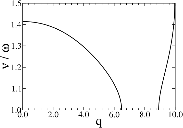
Figure 1: Canonical representative of the characteristic exponent $\nu$ for the Mathieu oscillator with parameter $a=8.0$, that is, for $\Omega_{0}/\omega=\sqrt{2}$, as function of the scaled driving strength $q=2\Omega_{1}^{2}/\omega^{2}$. The oscillator becomes unstable for $q\approx 6.49$, where $\nu/\omega=1$; then re-enters a regime of stability at $q\approx 8.91$, and becomes unstable again at $q\approx 9.97$, where $\nu/\omega=3/2$.

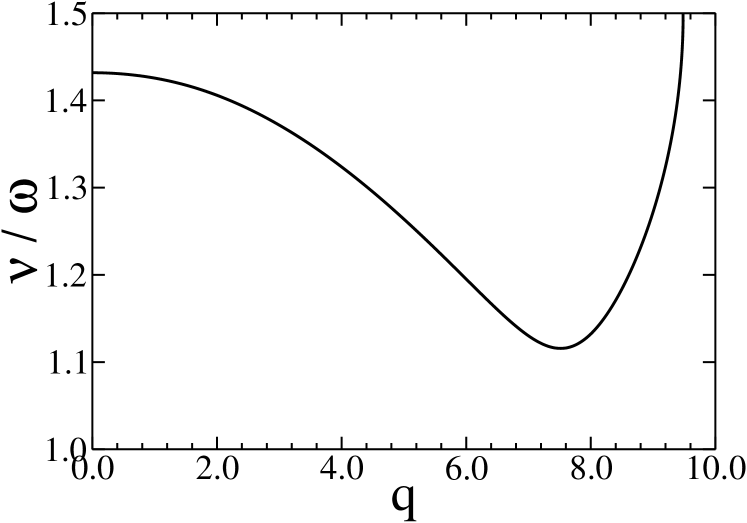
Figure 2: As Fig. 1, but for $a=4\Omega_{0}^{2}/\omega^{2}=8.2$. Here the oscillator becomes unstable for $q\approx 9.48$, where $\nu/\omega=3/2$.

The Figures 1 and 2 visualize the variation of the characteristic exponent with the scaled driving strength $q$ for $a=8.0$ and $a=8.2$, respectively; in view of Eq. (51) for the quasienergies, these Figures likewise depict the ac Stark shift exhibited by the quantum mechanical Mathieu oscillator.

It is of interest to observe that the classical Mathieu oscillator becomes mechanically unstable upon variation of $q$ in two different ways: Two complex eigenvalues $z_{\pm}=\exp(\pm{\mathrm{i}}\vartheta)$ of ${\bm{M}}$ collide on the unit circle and become real either when $z_{\pm}=+1$, so that $\vartheta=0$ and $\nu/\omega$ is integer, or when $z_{\pm}=-1$, giving $\vartheta=\pi$ and half-integer $\nu/\omega$. In the first case all quasienergies (51) of the corresponding quantum system are degenerate ($\bmod\;\hbar\omega$) at the transition point, whereas there are two separate groups of degenerate quasienergies, differing by $\hbar\omega/2$, in the second case, thus providing an elementary model for a Floquet time crystal ElseEtAl16 ; YaoEtAl17 . In fact, the transition from a stable to an unstable classical Mathieu oscillator corresponds to a transition from a pure point quasienergy spectrum to an absolutely continuous one for its quantum mechanical counterpart HagedornEtAl86 ; Combescure88 ; Howland92 . In a regime of stability each wave function possesses a representation as a superposition of the Floquet states constructed in Sec. II, and therefore evolves in time in a strictly quasiperiodic manner. In a regime of instability the solutions to the time-dependent Schrödinger equation are still associated with classical trajectories $\xi$, but these wave functions absorb an infinite amount of energy from the drive if their trajectories are unstable; such unbounded growth of energy is traced to the continuous quasienergy spectrum BunimovichEtAl91 .

IV Coupling to a thermal heat bath

Now let the parametrically driven “system” (1) with $T$-periodic spring function $k(t)$ be weakly coupled to a “bath” consisting of infinitely many harmonic oscillators with a prescribed temperature, causing transitions among the system’s Floquet states; our goal is to find the corresponding quasistationary distribution BreuerEtAl00 ; LangemeyerHolthaus14 ; SchmidtEtAl19 ; KetzmerickWustmann10 . Following the general theory of open quantum systems BreuerPetruccione02 we then require, besides the Hilbert space ${\mathcal{H}}_{\rm system}$ that the driven part $H_{0}(t)$ is acting on, the Hilbert space ${\mathcal{H}}_{\rm bath}$ pertaining to the bath Hamiltonian $H_{\rm bath}$, and construct the composite space ${\mathcal{H}}_{\rm system}\otimes{\mathcal{H}}_{\rm bath}$. Accordingly, the total Hamiltonian now takes the form

$$H(t)=H_{0}(t)\otimes\mathbbm{1}+\mathbbm{1}\otimes H_{\rm bath}+H_{\rm int}\;,$$ (61)

with

$$H_{\rm int}=V\otimes W$$ (62)

specifying the system-bath interaction. Here we choose a simple but plausible coupling mediated by

$$V=\gamma x\;,$$ (63)

where the constant $\gamma$ carries the dimension of energy per length, and

$$W=\sum_{\widetilde{\omega}}\left(b^{\phantom{\dagger}}_{\widetilde{\omega}}+b^{\dagger}_{\widetilde{\omega}}\right)\;,$$ (64)

effectuating annihilation and creation processes in the bath, with the sum ranging over all bath oscillators BreuerEtAl00 . Within a perturbative approach based on the golden rule for Floquet states BreuerEtAl00 ; LangemeyerHolthaus14 , a bath-induced transition from an initial Floquet state $i$ of the driven system to a final one labeled by $f$ does not correspond to only one single transition frequency, but rather to an infinite ladder of frequencies $\omega_{fi}^{(\ell)}$ differing from the expected frequency $(\varepsilon_{f}-\varepsilon_{i})/\hbar$ by positive or negative integer multiples of the driving frequency $\omega=2\pi/T$,

$$\omega_{fi}^{(\ell)}=(\varepsilon_{f}-\varepsilon_{i})/\hbar+\ell\omega\quad\text{with}\;\ell=0,\pm 1,\pm 2,\ldots\;;$$ (65)

note that a precise specification of the chosen quasienergy representatives is essential at this point. Hence, the rate $\Gamma_{fi}$ of such transitions is obtained as a sum,

$$\Gamma_{fi}=\sum_{\ell}\Gamma_{fi}^{(\ell)}\;,$$ (66)

where the partial rates $\Gamma_{fi}^{(\ell)}$ are given by

$$\Gamma_{fi}^{(\ell)}=\frac{2\pi}{\hbar^{2}}\left|V_{fi}^{(\ell)}\right|^{2}N(\omega_{fi}^{(\ell)})\,J(|\omega_{fi}^{(\ell)}|)\;.$$ (67)

Here the quantities $V_{fi}^{(\ell)}$ denote the Fourier coefficients of the system’s transition matrix elements,

$$\langle u_{f}(t)|V|u_{i}(t)\rangle=\sum_{\ell}{\mathrm{e}}^{{\mathrm{i}}\ell\omega t}\,V_{fi}^{(\ell)}\;.$$ (68)

The transition frequencies (65) can either be positive, as corresponding to processes during which the driven system absorbs energy from the bath, or negative, so that the system loses energy to the bath. Accordingly, the thermal averages $N(\widetilde{\omega})$ appearing in the partial rates (67) either refer to the de-excitation of a bath oscillator, that is, to the annihilation of a bath phonon,

$$N(\widetilde{\omega})\;=\;\langle n(\widetilde{\omega})\rangle\;=\;\frac{1}{\exp(\beta\hbar\widetilde{\omega})-1}$$ (69)

when $\widetilde{\omega}>0$, or to the creation of such a phonon,

$$N(\widetilde{\omega})\;=\;\langle n(-\widetilde{\omega})\rangle+1\;=\;\frac{1}{1-\exp(\beta\hbar\widetilde{\omega})}$$ (70)

when $\widetilde{\omega}<0$. Here we have written $n(\widetilde{\omega})=b^{\dagger}_{\widetilde{\omega}}b^{\phantom{\dagger}}_{\widetilde{\omega}}$ for the occupation number of a phonon mode, have employed angular brackets to indicate thermal averaging, and have used the familiar symbol $\beta=1/(k_{\rm B}T_{\rm bath})$ with the Boltzmann constant $k_{\rm B}$ to indicate the inverse of the bath temperature $T_{\rm bath}$. Finally, the factor $J(\widetilde{\omega})$ contributing to the partial rates (67) denotes the spectral density of the oscillator bath.

Having computed the matrix of transition rates (66) in this manner, the desired quasistationary distribution $\{p_{n}\}_{n=0,1,2,\ldots}$ which quantifies the system’s Floquet-state occupation probabilities in the non-equilibrium steady state is obtained as solution to the Pauli master equation BreuerEtAl00

$$\dot{p}_{n}=0=\sum_{m}\big{(}\Gamma_{nm}p_{m}-\Gamma_{mn}p_{n}\big{)}\;.$$ (71)

The decisive system-specific input data determining this quasistationary Floquet-state distribution are the Fourier coefficients of the transition matrix elements (68). With the dipole-type coupling (63), and again writing the decomposition of the $T$-periodic factor $v(t)$ of the classical Floquet solutions (40) as

$$v(t)=|v(t)|\exp\big{(}{\mathrm{i}}\widetilde{\alpha}(t)\big{)}$$ (72)

with $T$-periodic phase function $\widetilde{\alpha}(t)$, the quantum mechanical Floquet functions (50) of the parametrically driven harmonic oscillator provide the expression

$$\langle u_{m}(t)|x|u_{n}(t)\rangle = |v(t)|\left\langle u_{m}(t)\left|\frac{x}{|v(t)|}\right|u_{n}(t)\right\rangle$$ (73)

$$= \sqrt{\frac{\hbar}{2M\Omega}}\,|v(t)|\Big{(}\sqrt{n}\exp\!\big{(}-{\mathrm{i}}\widetilde{\alpha}(t)+{\mathrm{i}}\widetilde{\alpha}(0)\big{)}\,\delta_{m,n-1}+\sqrt{n+1}\exp\!\big{(}{\mathrm{i}}\widetilde{\alpha}(t)-{\mathrm{i}}\widetilde{\alpha}(0)\big{)}\,\delta_{m,n+1}\Big{)}$$

$$= \sqrt{\frac{\hbar}{2M\Omega}}\Big{(}\sqrt{n}\,v^{*}(t)\,{\mathrm{e}}^{{\mathrm{i}}\widetilde{\alpha}(0)}\,\delta_{m,n-1}+\sqrt{n+1}\,v(t)\,{\mathrm{e}}^{-{\mathrm{i}}\widetilde{\alpha}(0)}\,\delta_{m,n+1}\Big{)}\;.$$

Therefore, the required coefficients $V_{fi}^{(\ell)}$ of the expansion (68) are proportional to the Fourier coefficients of $v(t)$, which are easy to compute. Moreover, the transition matrix (66) becomes tridiagonal, having non-vanishing entries for $f=i\pm 1$ only. Thus, the master equation (71) simplifies considerably, reducing to

$$(\Gamma_{n,n-1}\,p_{n-1}-\Gamma_{n-1,n}\,p_{n})$$

$$+\;(\Gamma_{n,n+1}\,p_{n+1}-\Gamma_{n+1,n}\,p_{n}) = 0$$ (74)

for $n\geq 1$; for $n=0$ the first bracket disappears. This tridiagonal form implies detailed balance SchmidtEtAl19 , meaning that both brackets vanish individually for $n\geq 1$: Setting the second bracket to zero gives the forward relation

$$\frac{p_{n+1}}{p_{n}}=\frac{\Gamma_{n+1,n}}{\Gamma_{n,n+1}}$$ (75)

which already fixes the distribution $\{p_{n}\}_{n=0,1,2,\ldots}$ up to its normalization; shifting $n$ to $n-1$ in this relation (75) shows that Eq. (74) indeed is satisfied. Moreover, since $\Gamma_{n+1,n}$ and $\Gamma_{n,n+1}$ both are proportional to $n+1$ by virtue of Eq. (73), their ratio

$$\frac{\Gamma_{n+1,n}}{\Gamma_{n,n+1}}=r$$ (76)

actually is independent of $n$, resulting in the geometric Floquet-state distribution

$$p_{n}=(1-r)\,r^{n}\;$$ (77)

with the proviso that $r<1$, that is, provided the rate $\Gamma_{n+1,n}$ for each “upward” transition remains smaller than the rate $\Gamma_{n,n+1}$ of the matching “downward” transition. As in the case of a spin driven by a circularly polarized field SchmidtEtAl19 , the existence of such a geometric distribution (77), combined with equidistantly spaced canonical representatives (51) of the system’s quasienergies, now allows one to introduce a quasitemperature $\tau$ for the periodically driven nonequilibrium system: Setting

$$r=\exp\!\left(-\frac{\hbar\nu}{k_{\rm B}\tau}\right)\;,$$ (78)

one finds

$$\frac{\tau}{T_{\rm bath}}=-\frac{\hbar\nu}{k_{\rm B}T_{\rm bath}}\,\frac{1}{\ln r}\;.$$ (79)

This definition of the quasitemperature formally yields negative $\tau$ when $r>1$. While such negative quasitemperatures are quite natural and physically meaningful in systems with a finite-dimensional Hilbert space, such as periodically driven spin systems SchmidtEtAl19 , here they signal quasithermal instability, implying $\Gamma_{n+1,n}>\Gamma_{n,n+1}$, so that the particle tends to climb the oscillator ladder to infinite height.

Writing the Fourier series of $v(t)$ as

$$v(t)=\sum_{\ell}{\mathrm{e}}^{{\mathrm{i}}\ell\omega t}\,v^{(\ell)}\;,$$ (80)

one has, more explicitly,

$$r=\frac{\displaystyle{\sum_{\ell}}\left|v^{(\ell)}\right|^{2}\,N(+\nu+\ell\omega)\;J(|\nu+\ell\omega|)}{\displaystyle{\sum_{\ell}}\left|v^{(\ell)}\right|^{2}\,N(-\nu-\ell\omega)\;J(|\nu+\ell\omega|)}\;.$$ (81)

Let us now assume that the system approaches a mechanical stability border, such that $\nu/\omega$ tends to the integer $l_{0}$ from above, $\nu/\omega\to\ell_{0}$. In that case the Bose occupation numbers $N(+\nu-\ell_{0}\omega)=N(0+)$ and $N(-\nu+\ell_{0}\omega)=N(0-)$ both become singular according to their respective definition (69) or (70), with $N(0-)=N(0+)+1$. Hence, assuming further that the Fourier coefficient labeled $-\ell_{0}$ is of appreciable magnitude, and the spectral density $J(|\widetilde{\omega}|)$ smoothly approaches a nonvanishing value $J(0)$, both the numerator and the denominator of the expression (81) are practically exhausted by the term $\ell=-\ell_{0}$ alone, resulting in

$$r\approx\frac{N(0+)}{N(0+)+1}$$ (82)

and, hence, $r\to 1$, implying $\tau\to\infty$: If the (smooth) spectral density of the oscillator bath does not vanish at $\widetilde{\omega}=0$, the onset of mechanical instability for integer $\nu/\omega$ necessarily is accompanied by quasithermal instability.

Actually this link between mechanical and quasithermal instability is even closer: If the spring function $k(t)$ admits symmetric or antisymmetric functions $v(t)$ at the mechanical stability border, as it happens in the Mathieu case (57), one finds

$$\left|v^{(+\ell-\ell_{0})}\right|^{2}=\left|v^{(-\ell-\ell_{0})}\right|^{2}\quad{\rm if}\;\nu/\omega\to\ell_{0}\;,$$ (83)

or

$$\left|v^{(+\ell-\ell_{0})}\right|^{2}=\left|v^{(-\ell-\ell_{0}-1)}\right|^{2}\quad{\rm if}\;\nu/\omega\to\ell_{0}+1/2\;.$$ (84)

In both limiting cases the sums in the numerator and denominator of the ratio (81) become identical, so that the onset of mechanical instability entails $\tau=\infty$, even regardless of the bath density.

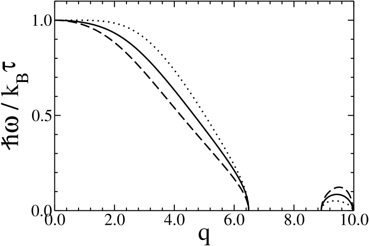
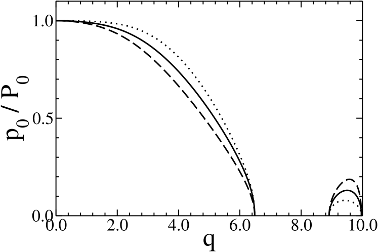
Figure 3: Scaled inverse quasitemperature $\hbar\omega/(k_{\rm B}\tau)$ (upper panel) and ratio $p_{0}/P_{0}$ (lower panel) of the occupation probability $p_{0}$ of the Floquet state $n=0$ to the occupation probability $P_{0}$ of the undriven system’s ground state for a Mathieu oscillator with $a=8.0$, as functions of the scaled driving strength $q$. The bath temperature corresponds to $\beta\hbar\omega=1$, while the spectral density of the bath is Ohmic ($s=1$, full lines), sub-Ohmic ($s=0.5$, dashed lines), and super-Ohmic ($s=2$, dotted lines). Observe that one has infinite quasitemperature at each mechanical stability border seen in Fig. 1.

For illustrating these deliberations we resort once again to the Mathieu oscillator (57), and now stipulate that the spectral density has the power-law form

$$J(\widetilde{\omega})=J_{0}\left(\frac{\widetilde{\omega}_{\phantom{0}}}{\widetilde{\omega}_{0}}\right)^{s}\;.$$ (85)

The case $s=1$ is designated as Ohmic BreuerPetruccione02 , so that exponents $0<s<1$ and $s>1$ indicate, respectively, sub-Ohmic and super-Ohmic densities. In Fig. 3 we display the scaled inverse quasitemperature $\hbar\omega/(k_{\rm B}\tau)$ as function of the scaled driving strength $q$ for all three cases, considering an oscillator with $a=8.0$ as in Fig. 1, while the bath temperature has been set to $\beta\hbar\omega=1.0$. We also plot the ratio $p_{0}/P_{0}$ of the quasithermal occupation probability

$$p_{0}=1-r$$ (86)

of the Floquet state $n=0$ to the thermal occupation probability of the undriven oscillator’s ground state,

$$P_{0}=1-\exp(-\beta\hbar\Omega_{0})\;.$$ (87)

Here the scaled inverse quasitemperature falls below the inverse bath temperature in both stable regions, implying that the driven system with $q>0$ effectively is hotter than the undriven one with $q=0$, so that the occupation probability of the Floquet state $n=0$ is lower than the occupation probability of the oscillator ground state in the absence of the drive, as might be expected naively on intuitive grounds. Moreover, each border of mechanical stability identified before in Fig. 1 precisely marks an onset of quasithermal instability, i.e., a driving strength for which $r=1$, or $\hbar\omega/(k_{\rm B}\tau)=0$.

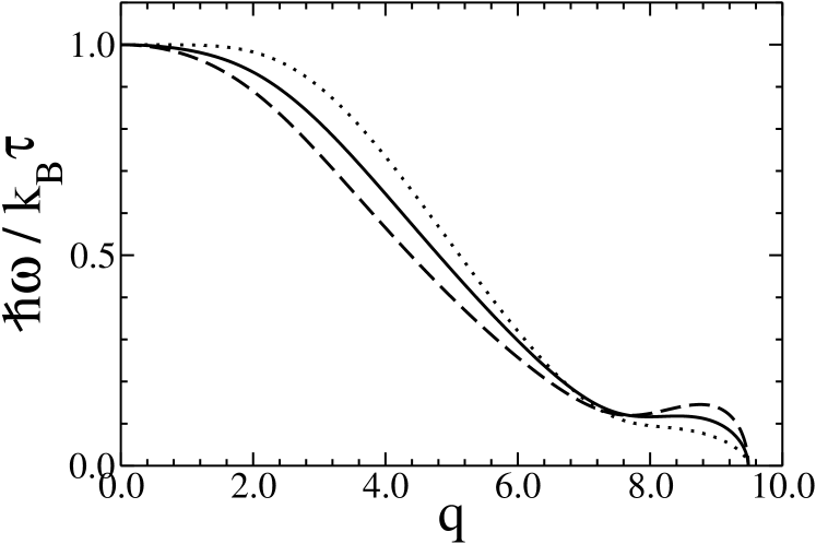
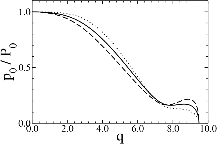
Figure 4: As Fig. 3, but for $a=8.2$. Observe that the sub-Ohmic density of states gives rise to a non-monotonic variation of the quasitemperature with the driving strength.

The corresponding data for $a=8.2$ are shown in Fig. 4. Here the sub-Ohmic density gives rise to a regime in which the inverse quasitemperature increases notably with increasing driving strength, similar to the second zone of stability in Fig. 3, indicating that the system can effectively become colder though the drive is made stronger, reflecting the behavior of the characteristic exponent depicted in Fig. 2.

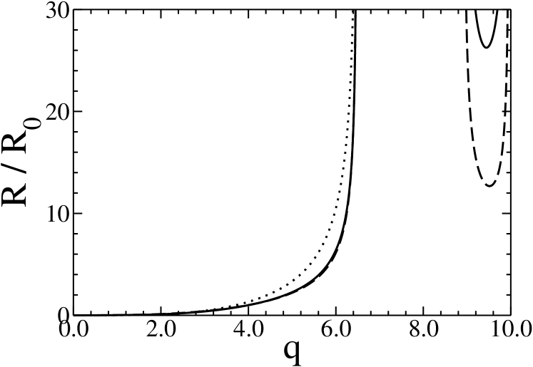
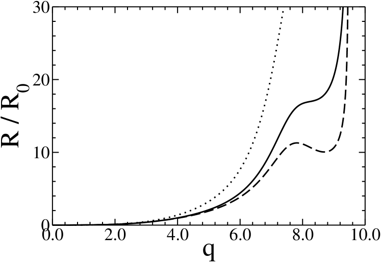
Figure 5: Scaled dissipation rates $R/R_{0}$ for a Mathieu oscillator with $a=8.0$ (upper panel) and $a=8.2$ (lower panel) as functions of the driving strength. As in Figs. 3 and 4, the bath temperature corresponds to $\beta\hbar\omega=1$, while the spectral density of the bath is Ohmic ($s=1$, full lines), sub-Ohmic ($s=0.5$, dashed lines), and super-Ohmic ($s=2$, dotted lines). The reference frequency entering the spectral densities (85) here is $\widetilde{\omega}_{0}/\omega=1.0$.

Since a Floquet transition of the system with negative (or positive) frequency $\omega_{mn}^{(\ell)}$ is accompanied by the addition (or subtraction) of the energy $-\hbar\omega_{mn}^{(\ell)}$ to (or from) the bath, the rate of energy dissipated in the quasistationary state is given by LangemeyerHolthaus14

$$R=-\sum_{mn\ell}\hbar\omega_{mn}^{(\ell)}\,\Gamma_{mn}^{(\ell)}\;p_{n}\;.$$ (88)

Utilizing $m=n\pm 1$ together with $\omega_{n\pm 1,n}^{(\ell)}=\pm\nu+\ell\omega$, and introducing the constant

$$c=\frac{\pi\gamma^{2}}{\hbar M\Omega}$$ (89)

which carries the dimension of squared inverse time, this dissipation rate (88) can be written as

$$R=R_{1}+R_{2}\;,$$ (90)

where

$$R_{1}=\frac{cr}{1-r}\sum_{\ell}\hbar|\nu+\ell\omega|\,\left|v^{(\ell)}\right|^{2}J(|\nu+\ell\omega|)$$ (91)

does not depend on the Bose occupation numbers (69) and (70), while the second contribution does not depend on $r$,

$$R_{2}=-c\sum_{\ell}\hbar(\nu+\ell\omega)\,\left|v^{(\ell)}\right|^{2}N(\nu+\ell\omega)\,J(|\nu+\ell\omega|)\;.$$ (92)

In the Appendix A we provide a formal proof of the intuitively expected, but non-obvious fact that this steady-state dissipation rate (88) is positive, so that the energy flow always is directed from the driven system into the bath, regardless of the system’s quasitemperature. In Fig. 5 we plot the dimensionless rate $R/R_{0}$, where the reference rate is taken as

$$R_{0}=\hbar\omega cJ_{0}\sum_{\ell}\left|v^{(\ell)}\right|^{2}\;,$$ (93)

for the situations previously considered in Figs. 3 and 4. Evidently the total dissipation rate is duly positive, and diverges at the borders of quasithermal stability, as predicted by the prefactor of the sum (91).

V Discussion: Quasithermal engineering

The numerical examples worked out in the preceding section all rely on the proposition that the bath-specific input determining the partial rates (67) and, hence, the quasistationary Floquet-state distributions $\{p_{n}\}_{n=0,1,2,\ldots}$, namely, the spectral density $J(\widetilde{\omega})$ be given by the models (85). With a view towards future applications of periodic thermodynamics this assumption may not be realistic; a given system may interact with its environment preferentially at certain distinguished frequencies. As will be demonstrated now, spectral densities structured in this manner may have remarkable physical effects. Consider, for instance, a Gaussian density

$$J(\widetilde{\omega})=J_{0}\exp\!\left(-\frac{(\widetilde{\omega}-\widetilde{\omega}_{0})^{2}}{(\Delta\widetilde{\omega})^{2}}\right)\;.$$ (94)

Given a sufficiently narrow width $\Delta\widetilde{\omega}$, and a central frequency $\widetilde{\omega}_{0}$ detuned not too far from one of the system’s positive “upward” transition frequencies $\omega^{(\ell_{1})}_{n+1,n}=\nu+\ell_{1}\omega$, this density (94) will essentially reduce the numerator and the denominator of the ratio (81) to the single contribution $\ell=\ell_{1}$, provided the accompanying squared Fourier coefficient is not too small, that is, if the drive is sufficiently strong. Since the transition frequencies enter into the density with their absolute value only, $J(|\nu+\ell_{1}\omega|)$ then cancels out of the remaining ratio, leaving us with

$$r\approx\frac{N(+\nu+\ell_{1}\omega)}{N(-\nu-\ell_{1}\omega)}\;.$$ (95)

Now the Bose occupation number $N(+\nu+\ell_{1}\omega)\equiv N_{+}$ is given by Eq. (69), whereas $N(-\nu-\ell_{1}\omega)=N_{+}+1$ is obtained from Eq. (70). If then additionally $N_{+}\ll 1$, one deduces $r\approx N_{+}/(N_{+}+1)\ll 1$ — meaning that the “downward” transitions can be strongly favored over the upward ones, even to the extent that the Floquet state $n=0$ is populated with higher probability than the oscillator ground state in the absence of the drive, or, expressed differently, that the quasitemperature of the driven system is lower than the temperature of the bath it is coupled to DiermannHolthaus19 .

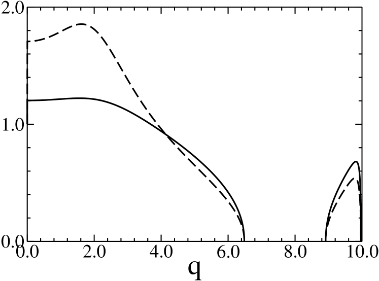
Figure 6: Scaled inverse quasitemperature $\hbar\omega/(k_{\rm B}\tau)$ (dashed) and occupation probability $p_{0}/P_{0}$ (full line) for the Mathieu oscillator with parameter $a=8.0$ coupled to a heat bath with $\beta\hbar\omega=1.0$ as in Fig. 3, but with a Gaussian spectral density (94) centered around $\widetilde{\omega}_{0}/\omega=3.2$, with squared width $(\Delta\widetilde{\omega}/\omega)^{2}=0.1$. Observe that the quasitemperature of the driven system is lower than the bath temperature for $0<q\lesssim 3.89$. (Both lines bend sharply at small $q$ unresolved here, and connect to the ordinate $1.0$ for $q=0$; see Fig. 7.)

To provide a working example of this counterintuitive “cooling by driving” mechanism, let us fix both the Mathieu parameter $a=8.0$ and the scaled bath temperature $\beta\hbar\omega=1.0$ to the values employed before, and let us select the parameters $(\Delta\widetilde{\omega}/\omega)^{2}=0.1$ and $\widetilde{\omega}_{0}/\omega=3.2$ for the above density (94). In view of Fig. 1, showing that the canonical representative of the characteristic exponent then varies in the interval $\sqrt{2}\geq\nu/\omega\geq 1.0$ within the first zone of stability, this selection tends to favor the contributions with $\ell=\ell_{1}=+2$ to the ratio (81), but to an extent depending on the scaled driving strength because of the ac Stark shift of $\nu$ with $q$. Numerical data corresponding to this scenario are displayed in Fig 6. Indeed, for $0<q\lesssim 3.89$ one finds $\hbar\omega/(k_{\rm B}\tau)>1$, implying $\tau<T_{\rm bath}$: The driven system effectively is cooled.

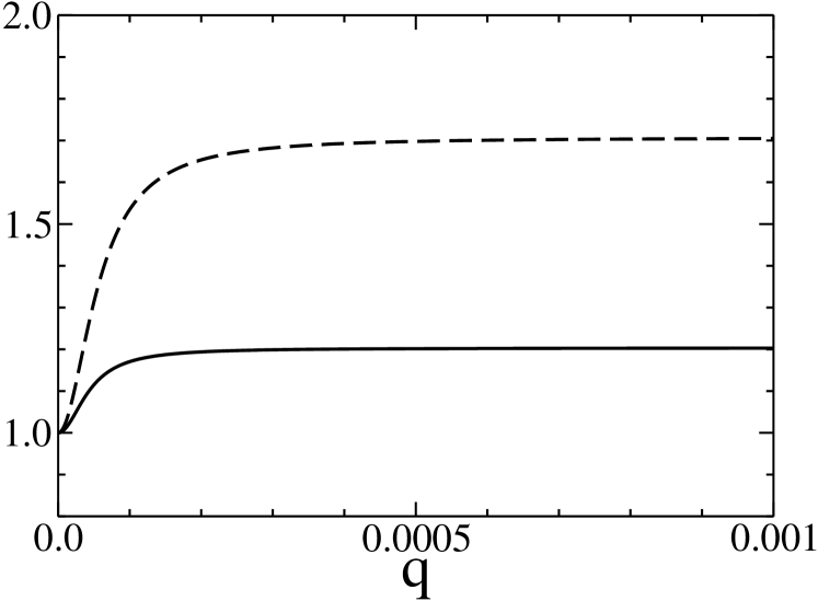
Figure 7: As Fig. 6, for small scaled driving strengths. The almost constant values of $\hbar\omega/(k_{\rm B}\tau)$ (dashed) and $p_{0}/P_{0}$ (full line) attained here are determined by Eq. (95) with $\ell_{1}=1$.

Seemingly, the lines drawn in Fig. 6 do not connect to the ordinate $1.0$ for vanishing $q$, as they should. But actually, they do: In Fig. 7 we magnify the behavior of both $\hbar\omega/(k_{\rm B}\tau)$ and $p_{0}/P_{0}$ for very small $q$, confirming the expected continuity for $q\to 0$. The plateau values adopted here are perfectly explained by Eq. (95) with $\ell_{1}=1$, as the higher Fourier coefficients are still too small to yield sizable contributions. This case study indicates that “cooling by driving” may work even with fairly low driving strengths, although the corresponding relaxation times to the quasithermal nonequilibrium steady state may be quite long if the rates are small.

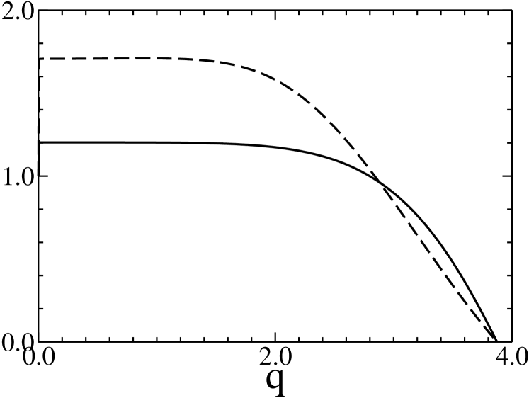
Figure 8: As Fig. 6, but with the Gaussian density (94) now being centered around $\widetilde{\omega}_{0}/\omega=3.0$. All other parameters have remained unchanged. Observe that the onset of quasithermal instability here has been decoupled from the mechanical instability identified in Fig. 1, occurring already at $q\approx 3.87$.

The possibilities to shape a quasistationary Floquet-state distribution with the help of the spectral density of the bath are by no means exhausted by this inaugural example of “quasithermal engineering”. Shifting the peak position from $\widetilde{\omega}_{0}/\omega=3.2$ to $\widetilde{\omega}_{0}/\omega=3.0$, but leaving all other parameters at their values already used for Fig. 6, one obtains the data visualized in Fig. 8: Here the onset of thermal instability already occurs for significantly lower driving strength $q\approx 3.87$ than the mechanical instability spotted in Fig. 1 at $q\approx 6.49$, and the system does not become quasithermally stable in the second regime of mechanical stability. This is no contradiction to our previous finding that $r\to 1$ at a mechanical stability border, since $r$ raises to values higher than $1.0$ already at $q\approx 3.87$, and then approaches unity from above.

Thus, the fact that quasistationary Floquet-state distributions do depend on the precise form of the system-bath coupling Kohn01 ; BreuerEtAl00 allows one to achieve unexpected effects by deliberately designing this coupling, that is, by quasithermal engineering. The phenomenon of “cooling by driving”, which reflects one particular application of this concept, bears interesting promises: If it were possible to decouple a driven system with a quasitemperature $\tau$ lower than the temperature $T_{\rm bath}$ of its bath from that bath, and then switch off the drive in an adiabatic manner so that the Floquet-state occupation probabilities would be preserved, the system would end up in state with a genuine temperature $\tau<T_{\rm bath}$ LangemeyerHolthaus14 .

The model system we have employed in the present study, the parametrically driven Mathieu oscillator, still is exceptionally simple from the Floquet point of view, not showing features which are characteristic for more generic non-integrable systems KetzmerickWustmann10 ; HoneEtAl09 . When dealing with such generic systems, one has to compute the Floquet states fully numerically in order to obtain the transition matrix elements (68) and their Fourier components, and then requires a numerical solution of the master equation (71), thus obstructing a clear view on the underlying physics. This is why simplicity is an outstanding virtue here. The only “hard” data required for converting predictions made by our model into numbers are the Fourier coefficients of the periodic parts (80) of the solutions to the classical equation of motion (8); even these coefficients can be obtained with fairly modest numerical effort. Therefore, the parametrically driven harmonic oscillator coupled to a thermal bath in various manners may serve as a valuable source of inspiration in the further exploration of periodic thermodynamics.

Appendix A Positivity of the dissipation rate

In this Appendix we demonstrate that the dissipation rate (88) is always positive, which implies that the energy flows from the driven oscillator into the bath when the system is in a quasistationary state, regardless of whether the system’s quasitemperature is higher or lower than the temperature of the bath it is coupled to. Accounting for $m=n\pm 1$ and $\omega_{n\pm 1,n}^{(\ell)}=\pm\nu+\ell\omega$, one has

$$R = -\sum_{n\ell}\hbar(+\nu+\ell\omega)\,\Gamma_{n+1,n}^{(\ell)}\;p_{n}$$ (96)

$$-\sum_{n\ell}\hbar(-\nu+\ell\omega)\,\Gamma_{n-1,n}^{(\ell)}\;p_{n}\;.$$

The proof of the positivity of $R$ rests on the observation that the contribution to this expression which is proportional to $\nu$ vanishes: We find

$$-\hbar\nu\sum_{n\ell}\Big{(}\Gamma_{n+1,n}^{(\ell)}-\Gamma_{n-1,n}^{(\ell)}\Big{)}p_{n}$$ (97)

$$= -\hbar\nu\sum_{n}\Big{(}\Gamma_{n+1,n}\;p_{n}-\Gamma_{n,n+1}\;p_{n+1}\Big{)}$$

$$= 0\;,$$

where, successively, the definition (66) and the detailed-balance relation (75) have been exploited. This allows us to replace $\nu$ in Eq. (96) by $\nu+\chi$, with arbitrary $\chi$. Therefore, the previous representation (90) involving the two expressions (91) and (92) can be cast into the form

$$R = \phantom{+}\hbar c\sum_{\nu+\ell\omega>0}\big{(}\nu+\ell\omega+\chi\big{)}\,\left|v^{(\ell)}\right|^{2}J(|\nu+\ell\omega|)\left(\frac{r}{1-r}-N(\nu+\ell\omega)\right)$$ (98)

$$+\hbar c\sum_{\nu+\ell\omega<0}\big{(}|\nu+\ell\omega|-\chi\big{)}\,\left|v^{(\ell)}\right|^{2}J(|\nu+\ell\omega|)\left(\frac{r}{1-r}+N(\nu+\ell\omega)\right)\;.$$

Now consider the last factor of the contributions to the first sum, namely,

$$\frac{r}{1-r}-N(\nu+\ell\omega)$$ (99)

$$= \frac{r\,\exp\!\big{(}\beta\hbar[\nu+\ell\omega]\big{)}-1}{(1-r)(\exp\!\big{(}\beta\hbar[\nu+\ell\omega]\big{)}-1)}\;.$$

Since $\nu+\ell\omega$ is positive here, both factors appearing in the denominator on the right-hand side are positive for a quasistationary state with $0<r<1$, while the numerator, which increases monotonically with $\ell$, may change its sign, being negative for $\ell<\ell_{0}$ and non-negative for $\ell\geq\ell_{0}$. Let us then select $\chi\leq 0$ such that the factor $\nu+\ell\omega+\chi$ is negative for $\ell<\ell_{0}$, but positive for $\ell\geq\ell_{0}$. Then all terms contributing to the first sum in Eq. (98) are non-negative, while the second sum is manifestly positive for $\chi\leq 0$. This concludes the proof.

References

- (1) L. D. Landau and E. M Lifshitz, Statistical Physics, Part 1. Course of Theoretical Physics, Volume 5 (Pergamon, Oxford, 1980).
- (2) F. Reif, Fundamentals of Statistical and Thermal Physics (Waveland Press, Long Grove, 2009).
- (3) R. K. Pathria and Paul D. Beale, Statistical Mechanics, third edition (Butterworth-Heinemann, Oxford, 2011).
- (4) W. Kohn, Periodic Thermodynamics, J. Stat. Phys. 103, 417 (2001).
- (5) H.-P. Breuer, W. Huber, and F. Petruccione, Quasistationary distributions of dissipative nonlinear quantum oscillators in strong periodic driving fields, Phys. Rev. E 61, 4883 (2000).
- (6) T. Shirai, T. Mori, and S. Miyashita, Condition for emergence of the Floquet-Gibbs state in periodically driven open systems, Phys. Rev. E 91, 030101(R) (2015).
- (7) Dong E. Liu, Classifiction of the Floquet statistical distribution for time-periodic open systems, Phys. Rev. B 91, 144301 (2015).
- (8) M. Langemeyer and M. Holthaus, Energy flow in periodic thermodynamics, Phys. Rev. E 89, 012101 (2014).
- (9) H.-J. Schmidt, J. Schnack, and M. Holthaus, Periodic thermodynamics of the Rabi model with circular polarization for arbitrary spin quantum numbers, arXiv:1902.05814.
- (10) R. Ketzmerick and W. Wustmann, Statistical mechanics of Floquet systems with regular and chaotic states, Phys. Rev. E 82, 021114 (2010).
- (11) D. Vorberg, W. Wustmann, R. Ketzmerick, and A. Eckardt, Generalized Bose-Einstein condensation into multiple states in driven-dissipative systems, Phys. Rev. Lett. 111, 240405 (2013).
- (12) A. Schnell, R. Ketzmerick, and A. Eckardt, On the number of Bose-selected modes in driven-dissipative ideal Bose gases, Phys. Rev. E 97, 032136 (2018).
- (13) K. Husimi, Miscellanea in elementary quantum mechanics, II, Prog. Theor. Phys. 9, 381 (1953).
- (14) H. R. Lewis and W. B. Riesenfeld, An exact quantum theory of the time-dependent harmonic oscillator and of a charged particle in a time-dependent electromagnetic field, J. Math. Phys. 10, 1458 (1969).
- (15) V. S. Popov and A. M. Perelomov, Parametric excitation of a quantum oscillator, Sov. Phys. JETP 29, 738 (1969) [Zh. Eksp. Teor. Fiz. 56, 1375 (1969)].
- (16) V. S. Popov and A. M. Perelomov, Parametric excitation of a quantum oscillator II, Sov. Phys. JETP 30, 910 (1970) [Zh. Eksp. Teor. Fiz. 57, 1684 (1969)].
- (17) M. Combescure, A quantum particle in a quadrupole radio-frequency trap, Ann. Inst. Henri Poincaré 44, 293 (1986).
- (18) L. S. Brown, Quantum motion in a Paul trap, Phys. Rev. Lett. 66, 527 (1991).
- (19) W. Miller, Symmetry Groups and their Applications (Academic Press, New York, 1972), pp 159–161.
- (20) J. V. José and E. J. Saletan, Classical Dynamics: A Contemporary Approach (Cambridge University Press, Cambridge, 1998).
- (21) W. Magnus, S. Winkler, Hill’s Equation (Dover Publications, Mineola, New York, 2004).
- (22) M. Abramowitz and I. A. Stegun (eds.), Handbook of Mathematical Functions (Dover Publications, New York, 1970).
- (23) W. Paul und H. Steinwedel, Ein neues Massenspektrometer ohne Magnetfeld, Z. Naturforschg. 8a, 448 (1953).
- (24) H. Dehmelt, Experiments with an isolated subatomic particle at rest, Rev. Mod. Phys. 62, 525 (1990).
- (25) W. Paul, Electromagnetic traps for charged and neutral particles, Rev. Mod. Phys. 62, 531 (1990).
- (26) D. V. Else, B. Bauer, and C. Nayak, Floquet time crystals, Phys. Rev. Lett. 117, 090402 (2016).
- (27) N. Y. Yao, A. C. Potter, I.-D. Potirniche, and A. Vishwanath, Discrete time crystals: Rigidity, criticality, and realizations, Phys. Rev. Lett. 118, 030401 (2017).
- (28) G. A. Hagedorn, M. Loss, and J. Slawny, Non-stochasticity of time-dependent quadratic Hamiltonians and the spectra of canonical transformations, J. Phys. A: Math. Gen. 19, 521 (1986).
- (29) M. Combescure, The quantum stability problem for some class of time-dependent Hamiltonians, Ann. Phys. (N.Y.) 185, 86 (1988).
- (30) J. S. Howland, Quantum stability. In: Schrödinger operators: The quantum mechanical many-body problem. Lecture Notes in Physics 403, p. 100 (Springer, Berlin, 1992).
- (31) L. Bunimovich, H. R. Jauslin, J. L. Lebowitz, A. Pellegrinotti, and P. Nielaba, Diffusive energy growth in classical and quantum driven oscillators, J. Stat. Phys. 62, 793 (1991).
- (32) H.-P. Breuer and F. Petruccione, The Theory of Open Quantum Systems (Oxford University Press, Oxford, 2002).
-
(33)
O. R. Diermann and M. Holthaus,
Floquet-state cooling,
Scientific Reports 9, Article number: 17614 (2019).
Available online at www.nature.com/articles/s41598-019-53877-w - (34) D. W. Hone, R. Ketzmerick, and W. Kohn, Statistical mechanics of Floquet systems: The pervasive problem of near degeneracies, Phys. Rev. E. 79, 051129 (2009).