On the Stability of Lagrange Relative Equilibrium in the Planar Three-body Problem

Abstract

Since the strong degeneracies present in the N-body problem, even in the basic case of the planar three-body problem, nobody inspects the problem of nonlinear stability of Lagrange relative equilibrium. We introduce a new coordinate system to reduce degeneracies according to intrinsic symmetrical characteristic of the $N$-body problem, then we prove that Lagrange relative equilibrium is stable in the sense of measure, provided it is spectrally stable and except six special resonant cases. Indeed, under this condition, there are abundant KAM invariant tori or quasi-periodic solutions near Lagrange relative equilibrium. Furthermore, these tori or quasi-periodic solutions form a set whose relative measure rapidly tends to 1. We also prove that Lagrange relative equilibrium is exponentially stable for almost every choice of masses in the sense of measure, provided it is spectrally stable; and topologically, this is also right for a large open subset of spectrally stable space of masses.

Key Words: N-body problem; Relative equilibrium; Stability; Central configurations; KAM; Nekhoroshev theory; Normal Forms.

2010AMS Subject Classification 70F10 34D20 70H14 70K20 70F15 70K45.

1 Introduction

We consider $N$ particles with positive mass moving in an Euclidean space ${\mathbb{R}}^{2}$ interacting under the laws of universal gravitation. Let the $k$-th particle have mass $m_{k}$ and position $\mathbf{r}_{k}\in{\mathbb{R}}^{2}$ ($k=1,2,\cdots,N$), then the equation of motion of the $N$-body problem is written

$$m_{k}\ddot{\mathbf{r}}_{k}=\sum_{1\leq j\leq N,j\neq k}\frac{m_{k}m_{j}(\mathbf{r}_{j}-\mathbf{r}_{k})}{|\mathbf{r}_{j}-\mathbf{r}_{k}|^{3}},~{}~{}~{}~{}~{}~{}~{}~{}~{}~{}~{}~{}~{}~{}~{}k=1,2,\cdots,N.$$ (1.1)

where $|\cdot|$ denotes the Euclidean norm in ${\mathbb{R}}^{2}$. Since these equations are invariant by translation, we can assume that the center of mass stays at the origin.

The problem of stability of motion of the $N$-body problem is one of the major problems in mathematics or even in science. However, there are various stability concepts in modern literature, e.g., Lyapunov stability, Lagrange stability, Poisson stability, linear stability, spectral stability, orbital stability, effective stability and stability in the sense of measure (i.e., KAM stability) etc. Beyond doubt, Lyapunov stability is what we all want most and the most difficult to obtain. Note that orbital stability is essentially a kind of stability in the sense of Lyapunov.

For the $N$-body problem, the first result on stability was due to Laplace and Lagrange: the Laplace theorem on the absence of secular perturbations of the semiaxes. The result was on the stability of the solar system in the sense of Lagrange stability. The method of Laplace is a perturbation analysis neglecting terms in the mass of second-order and higher. Then Poisson and Jacobi extended the perturbation analysis to third-order terms in the mass, and concluded that Lagrange stability of the solar system is not guaranteed by the method the truncation of the order in the perturbation analysis.

Next major breakthrough is the well known Arnold’s theorem [4, 12, 8], a success of modern celebrated KAM theory, which claims that: for sufficiently small masses of the planets, Lagrange stability of the solar system is guaranteed for a set of positive Lebesgue measure of initial conditions. In particular, in the planar restricted circular three-body problem, by the well known Kolmogorov-Arnold’s theorem [1], if the mass of Jupiter is sufficiently small, then the motion of the the asteroid is stable in the sense of Lagrange stability for most of the initial conditions.

Since the independent work of Gascheau in 1843 [13] and Routh in 1875 [37] on linear stability of Lagrange relative equilibrium of the three-body problem, there are a good deal of work on linear stability of the $N$-body problem, please see [26, 35, 36, 24, 19, 18, etc] and the references therein.

The problem of Lyapunov stability has been solved only for Lagrange relative equilibrium in the planar restricted circular three-body problem, by a great amount of work based upon KAM theory in the 1970s. Please see [10, 20, 23, 38, 25, etc] and the references therein. However, due to the possibility of the well known Arnold diffusion, the method has the limitation that, the number of degrees of freedom of the problem is not more than 2.

For physical application, it is natural to consider a sort of “effective stability”, i.e., stability up to finite but long times. More precisely, for any solution $q(t)$ of a system, with initial condition in a small $\epsilon$-neighbourhood of the equilibrium point $q_{0}$ of the system, one could guaranty the estimate $|q(t)-q_{0}|=O(\epsilon^{a})$ for all times $|t|\leq T(\epsilon)$, where $a$ is some positive number in the interval $(0,1)$, and $T(\epsilon)$ is a “large” time such that $T(\epsilon)=O(\frac{1}{\epsilon^{b}})$ or even more stronger $T(\epsilon)\sim exp(\frac{1}{\epsilon^{b}})$ for some positive number $b$. The latter stronger form of stability is well known as exponential stability. The exponential stability was first stated by Moser [27] and Littlewood [22, 21] in particular cases. A general framework in this direction was developed by Nekhoroshev [29]. Then a great amount of work focus on the effective stability of Lagrange relative equilibrium in the planar or spatial restricted circular three-body problem, please see [16, 7, 17, 5, 15, etc] and the references therein. As a matter of fact, the stability over long times has been investigated by Birkhoff [6] using the method of normal form going back to Poincaré.

Although a great amount of work on stability has been done, however, even in the basic case of the planar three-body problem, it seems that nobody consider the problem of nonlinear stability of Lagrange relative equilibrium. One of the reason may be that one could not reduce the degeneracy of the equations of motion caused by integral of the $N$-body problem well. Inspired by the work on the problem of the infinite spin [40], we find that the so-called moving coordinates introduced in [40] are suitable for describing orbits near central configurations in the planar $N$-body problem, so it is natural to utilize the moving coordinates to investigate stability of relative equilibria. In the moving coordinates, the degeneracy of the equations of motion according to intrinsic symmetrical characteristic of the $N$-body problem can easily be reduced. In fact, one can simply reduce the degeneracy corresponding to rotation symmetry of the $N$-body problem, and obtain practical equations of motion in a small neighbourhood of a relative equilibrium. This is one important reason we can investigate nonlinear stability of relative equilibria.

The paper is structured as follows. In Section 2, we recall some notations, and some preliminary results including the moving coordinates in [40], and give equations of motion by the moving coordinates. In Section 3, we simply discuss orbital and linear stability of relative equilibria of the planar $N$-body problem, to prepare for investigating KAM stability and effective stability of Lagrange relative equilibrium in the planar three-body problem. In Section 4, we recall some necessary classical aspects of Hamiltonian system. In Section 5, we give the Birkhoff normal form of the Hamiltonian near Lagrange triangular point. Although the construction of the normal form is simple in concept but technically complicated in operations, which require some computer assistance; the analysis was performed with the aid of Mathematica. In Section 6, we investigate KAM stability of Lagrange relative equilibrium, in particular, it is shown that there are a great quantity of quasi-periodic solutions in a small neighbourhood of Lagrange relative equilibrium. Finally, in Section 7, we investigate effective stability of Lagrange relative equilibrium.

2 Preliminaries

In this section we recall some notations and definitions given in [40]. In particular, we recall the so-called moving coordinates introduced to study collision orbits in [40], which would be quite useful for the investigation of the stability of relative equilibrium solutions.

Let $(\mathbb{R}^{2})^{N}$ denote the space of configurations for $N$ point particles in Euclidean space $\mathbb{R}^{2}$: $(\mathbb{R}^{2})^{N}=\{\mathbf{r}=(\mathbf{r}_{1},\cdots,\mathbf{r}_{N}):\mathbf{r}_{j}\in\mathbb{R}^{2},j=1,\cdots,N\}$. We remark that, when necessary, one may identify $\mathbb{R}^{2}$ with $\mathbb{C}$ and $(\mathbb{R}^{2})^{N}$ with $\mathbb{C}^{N}$ and so on; in particular, $\mathbf{S}^{1}=\{e^{\mathbf{i}\theta}|\theta\in\mathbb{R}\}$, the unit circle in $\mathbb{C}$, is identified with the special orthogonal group $S\mathbb{O}(2)$ of the plane, where $\mathbf{i}$ is the imaginary unit. Thus, for a configuration $\mathbf{r}\in(\mathbb{R}^{2})^{N}$ and a complex number $\textsf{z}\in\mathbb{C}$, $\textsf{z}\mathbf{r}$ is defined by

$\textsf{z}\mathbf{r}:=(\textsf{z}\mathbf{r}_{1},\textsf{z}\mathbf{r}_{2},\cdots,\textsf{z}\mathbf{r}_{N})$,

and $\mathbf{i}\mathbf{r}$ is just $\mathbf{r}$ rotated anticlockwise by an angle $\frac{\pi}{2}$. Here and below, please refer to [40] for more detail. In this paper, unless otherwise specified, every vector is considered as a column vector.

For two configurations $\mathbf{r}=(\mathbf{r}_{1},\cdots,\mathbf{r}_{N})$ and $\mathbf{s}=(\mathbf{s}_{1},\cdots,\mathbf{s}_{N})$ in $(\mathbb{R}^{2})^{N}$, their mass scalar product is defined as:

$$\langle\mathbf{r},\mathbf{s}\rangle=\sum_{j=1}^{N}{{m_{j}(\mathbf{r}_{j},\mathbf{s}_{j})}}=\mathbf{r}^{\top}\mathfrak{M}\mathbf{s},$$

where $(\cdot,\cdot)$ denotes the standard scalar product in $\mathbb{R}^{2}$, $\mathfrak{M}$ is the diagonal matrix

$diag(m_{1},m_{1},m_{2},m_{2},\cdots,m_{N},m_{N})$,

and “$\top$” denotes transposition of matrix. We denote $\|\cdot\|$ the Euclidean norm associated to the mass scalar product, that is

$$\|\mathbf{r}\|=\sqrt{\langle\mathbf{r},\mathbf{r}\rangle}.$$

Then the cartesian space $(\mathbb{R}^{2})^{N}$ is a new Euclidean space.

Recall that, the moment of inertia, the kinetic energy, the opposite of the potential energy (force function), the total energy, the angular momentum, and the Lagrangian function are respectively defined as

$$I(\mathbf{r})=\sum_{j=1}^{N}{{m_{j}|{\mathbf{r}}_{j}-{\mathbf{r}}_{c}|^{2}}}.$$

$$\mathcal{K}(\dot{\mathbf{r}})=\sum_{j=1}^{N}{\frac{1}{2}{m_{j}|\dot{\mathbf{r}}_{j}|^{2}}},$$

$$\mathcal{U}(\mathbf{r})=\sum_{1\leq k<j\leq N}{\frac{m_{k}m_{j}}{|\mathbf{r}_{k}-\mathbf{r}_{j}|}},$$

$$\mathcal{H}(\mathbf{r},\dot{\mathbf{r}})=\mathcal{K}(\dot{\mathbf{r}})-\mathcal{U}(\mathbf{r}),$$

$$\mathcal{J}(\mathbf{r})=\sum_{j=1}^{N}{m_{j}{\mathbf{r}}_{j}\times{\dot{\mathbf{r}}}_{j}},$$

$$\mathcal{L}(\mathbf{r},\dot{\mathbf{r}})=\mathcal{L}=\mathcal{K}+\mathcal{U}=\sum_{j}\frac{1}{2}m_{j}|\dot{\mathbf{r}}_{j}|^{2}+\sum_{k<j}{\frac{m_{k}m_{j}}{|\mathbf{r}_{k}-\mathbf{r}_{j}|}},$$

where $|\cdot|$ denotes the Euclidean norm in ${\mathbb{R}}^{2}$, $\times$ denotes the standard cross product in $\mathbb{R}^{2}$, and $\mathbf{r}_{c}=\frac{\sum_{k=1}^{N}{m_{k}\vec{r}_{k}}}{\sum_{k=1}^{N}{m_{k}}}$ is the center of mass.

Without loss of generality, one assumes that the center of mass is fixed at the origin. Let $\mathcal{X}$ denote the space of configurations whose center of mass is at the origin; that is, $\mathcal{X}=\{\mathbf{r}=(\mathbf{r}_{1},\cdots,\mathbf{r}_{N})\in(\mathbb{R}^{2})^{N}:\sum_{k=1}^{N}{m_{k}\mathbf{r}_{k}}=0\}$, or,

$$\mathcal{X}=\{\mathbf{r}\in(\mathbb{R}^{2})^{N}:\langle\mathbf{r},\mathcal{E}_{2N-1}\rangle=0,\langle\mathbf{r},\mathcal{E}_{2N}\rangle=0\},$$

where

$$\mathcal{E}_{2N-1}=(1,0,\cdots,1,0)^{\top},\mathcal{E}_{2N}=(0,1,\cdots,0,1)^{\top}.$$

Thus

$$(\mathbb{R}^{2})^{N}=span\{\mathcal{E}_{2N-1},\mathcal{E}_{2N}\}\oplus\mathcal{X}.$$

Note that, for a configuration $\mathbf{r}\in\mathcal{X}$, we have

$$\|\mathbf{r}\|=\sqrt{I(\mathbf{r})}.$$

Let $\Delta$ be the collision set in $(\mathbb{R}^{2})^{N}$, that is, $\Delta=\{\mathbf{r}\in(\mathbb{R}^{2})^{N}:\mathbf{r}_{j}=\mathbf{r}_{k}~{}\text{for some}~{}j<k\}$. Then the set $\mathcal{X}\backslash\Delta$ is the space of collision-free configurations.

Let us recall the important concept of the central configuration:

Definition 2.1

A configuration $\mathbf{r}\in\mathcal{X}\backslash\Delta$ is called a central configuration if there exists a constant $\lambda\in{\mathbb{R}}$ such that

$$\sum_{j=1,j\neq k}^{N}\frac{m_{j}m_{k}}{|\mathbf{r}_{j}-\mathbf{r}_{k}|^{3}}(\mathbf{r}_{j}-\mathbf{r}_{k})=-\lambda m_{k}\mathbf{r}_{k},1\leq k\leq N.$$ (2.2)

The value of $\lambda$ in (2.2) is uniquely determined by

$$\lambda=\frac{\mathcal{U}(\mathbf{r})}{I(\mathbf{r})}.$$ (2.3)

It is well known that a central configuration is just a critical point of the normalized potential $\widetilde{\mathcal{U}}:=I^{\frac{1}{2}}\mathcal{U}$. Moreover, a central configuration $\mathbf{r}_{0}$ will be called nondegenerate, if the kernel of $D^{2}\widetilde{\mathcal{U}}(\mathbf{r}_{0})$, the Hessian of $\widetilde{\mathcal{U}}$ evaluated at $\mathbf{r}_{0}$, is exactly the plane $\mathcal{P}_{\mathbf{r}_{0}}$, where

$\mathcal{P}_{\mathbf{r}_{0}}:=\{\textsf{z}\mathbf{r}_{0}|\textsf{z}\in\mathbb{C}\}=span\{\mathbf{r}_{0},\mathbf{i}\mathbf{r}_{0}\}$.

Let $\mathcal{P}^{\bot}_{\mathbf{r}_{0}}$ be the orthogonal complement of $\mathcal{P}_{\mathbf{r}_{0}}$ in $\mathcal{X}$, that is,

$$\mathcal{X}=\mathcal{P}_{\mathbf{r}_{0}}\oplus\mathcal{P}^{\bot}_{\mathbf{r}_{0}},$$

then $\mathcal{P}^{\bot}_{\mathbf{r}_{0}}$, $\mathcal{P}_{\mathbf{r}_{0}}$ and $span\{\mathcal{E}_{2N-1},\mathcal{E}_{2N}\}$ are three invariant subspaces of $D^{2}\widetilde{\mathcal{U}}(\mathbf{r}_{0})$. Note that $\mathcal{E}_{2N-3}:=\mathbf{r}_{0}$, $\mathcal{E}_{2N-2}:=\mathbf{i}\mathbf{r}_{0}$, $\mathcal{E}_{2N-1}$ and $\mathcal{E}_{2N}$ are four eigenvectors of the Hessian $D^{2}\widetilde{\mathcal{U}}(\mathbf{r}_{0})$. By considering eigenvectors of the Hessian $D^{2}\widetilde{\mathcal{U}}(\mathbf{r}_{0})$, it follows that there is an orthogonal basis

$\{\mathcal{E}_{1},\mathcal{E}_{2},\cdots,\mathcal{E}_{2N-5},\mathcal{E}_{2N-4},\mathcal{E}_{2N-3},\mathcal{E}_{2N-2}\}$

of $\mathcal{X}$ such that

$\mathcal{P}^{\bot}_{\mathbf{r}_{0}}=span\{\mathcal{E}_{1},\mathcal{E}_{2},\cdots,\mathcal{E}_{2N-5},\mathcal{E}_{2N-4}\}$,

Assume

$$D^{2}\widetilde{\mathcal{U}}(\mathbf{r}_{0})\mathcal{E}_{j}=\lambda_{j}\mathcal{E}_{j},~{}~{}~{}~{}~{}~{}~{}~{}~{}~{}~{}~{}j=1,\cdots,2N,$$ (2.4)

then $\lambda_{2N-3}=\lambda_{2N-2}=0$ and $\lambda_{2N-1}=\lambda_{2N}=I^{\frac{1}{2}}\lambda$.

As a matter of fact, a straightforward computation shows that the Hessian $D^{2}\widetilde{\mathcal{U}}(\mathbf{r}_{0})$ with respect to the mass scalar product in $(\mathbb{R}^{2})^{N}$ is

$$I^{\frac{1}{2}}(\lambda\mathbb{I}+\mathfrak{M}^{-1}\mathfrak{B})-3I^{-\frac{1}{2}}\lambda\mathbf{r}_{0}\mathbf{r}_{0}^{\top}\mathfrak{M},$$

thus

$$\left(I^{\frac{1}{2}}(\lambda\mathbb{I}+\mathfrak{M}^{-1}\mathfrak{B})-3I^{-\frac{1}{2}}\lambda\mathbf{r}_{0}\mathbf{r}_{0}^{\top}\mathfrak{M}\right)\mathcal{E}_{j}=\lambda_{j}\mathcal{E}_{j},~{}~{}~{}~{}~{}~{}~{}~{}~{}~{}~{}~{}j=1,\cdots,2N.$$ (2.5)

Where $I=I(\mathbf{r}_{0})=\|\mathbf{r}_{0}\|^{2}$, $\lambda=\frac{\mathcal{U}(\mathbf{r}_{0})}{I(\mathbf{r}_{0})}$, $\mathfrak{B}$ is the Hessian of $\mathcal{U}$ evaluated at $\mathbf{r}_{0}$ with respect to the standard scalar product of $(\mathbb{R}^{2})^{N}$ and can be viewed as an $N\times N$ array of $2\times 2$ blocks:

$\mathfrak{B}=\left(\begin{array}[]{ccc}B_{11}&\cdots&B_{1N}\\ \vdots&\ddots&\vdots\\ B_{N1}&\cdots&B_{NN}\\ \end{array}\right).$

The off-diagonal blocks are given by:

$B_{jk}=\frac{m_{j}m_{k}}{r^{3}_{jk}}[\mathbb{I}-\frac{3(\mathbf{r}_{k}-\mathbf{r}_{j})(\mathbf{r}_{k}-\mathbf{r}_{j})^{\top}}{r^{2}_{jk}}],$

the diagonal blocks are given by:

$$B_{kk}=-\sum_{1\leq j\leq N,j\neq k}B_{jk},$$

where $r_{jk}=|\mathbf{r}_{k}-\mathbf{r}_{j}|$. Note that, as a matter of notational convenience, the identity matrix of any order will always be denoted by $\mathbb{I}$, and the order of $\mathbb{I}$ can be determined according to the context.

By (2.5), it follows that

$$(\lambda\mathbb{I}+\mathfrak{M}^{-1}\mathfrak{B})(\mathcal{E}_{1},\cdots,\mathcal{E}_{2N})=(\mathcal{E}_{1},\cdots,\mathcal{E}_{2N})diag(\frac{\lambda_{1}}{\|\mathbf{r}_{0}\|},\cdots,\frac{\lambda_{2N-4}}{\|\mathbf{r}_{0}\|},3\lambda,0,\lambda,\lambda).$$ (2.6)

That is, the orthogonal basis $\{\mathcal{E}_{1},\cdots,\mathcal{E}_{2N}\}$ and the corresponding eigenvalues $\lambda_{1},\cdots,\lambda_{2N}$ can be obtained by calculating eigenvectors of the matrix $\lambda\mathbb{I}+\mathfrak{M}^{-1}\mathfrak{B}$.

Given a configuration $\mathbf{r}$, let $\hat{\mathbf{r}}:=\frac{\mathbf{r}}{\|\mathbf{r}\|}$ be the unit vector corresponding to $\mathbf{r}$ henceforth. In particular, the unit vector $\hat{\mathbf{r}}$ is called the normalized configuration of the configuration $\mathbf{r}$.

Then

$$\{\hat{\mathcal{E}}_{1},\hat{\mathcal{E}}_{2},\hat{\mathcal{E}}_{3},\hat{\mathcal{E}}_{4},\cdots,\hat{\mathcal{E}}_{2N}\}$$

consisting of eigenvectors of $D^{2}\widetilde{\mathcal{U}}(\mathbf{r}_{0})$ is a standard orthogonal basis of the space $(\mathbb{R}^{2})^{N}$ with respect to the scalar product $\langle,\rangle$, that is,

$$(\hat{\mathcal{E}}_{1},\hat{\mathcal{E}}_{2},\hat{\mathcal{E}}_{3},\hat{\mathcal{E}}_{4},\cdots,\hat{\mathcal{E}}_{2N})^{\top}\mathfrak{M}(\hat{\mathcal{E}}_{1},\hat{\mathcal{E}}_{2},\hat{\mathcal{E}}_{3},\hat{\mathcal{E}}_{4},\cdots,\hat{\mathcal{E}}_{2N})=\mathbb{I}.$$

2.1 Moving Coordinates

Let us recall the so-called moving coordinates introduced in [40]. The moving coordinates are appropriate to describe the orbits near a central configuration. Here we say a configuration $\mathbf{r}\in\mathcal{X}$ is near the given central configuration $\mathbf{r}_{0}$, if $\mathbf{r}\notin\mathcal{P}^{\bot}_{\mathbf{r}_{0}}$.

For any configuration $\mathbf{r}\in\mathcal{X}\backslash\mathcal{P}^{\bot}_{\mathbf{r}_{0}}$, it is easy to see that there exists a unique point $e^{\mathbf{i}\theta(\mathbf{r})}\hat{\mathbf{r}}_{0}$ on the circle $\mathbf{S}:=\{e^{\mathbf{i}\theta}\hat{\mathbf{r}}_{0}|\theta\in\mathbb{R}\}$ such that

$$\|e^{\mathbf{i}\theta(\mathbf{r})}\hat{\mathbf{r}}_{0}-\mathbf{r}\|=min_{\theta\in\mathbb{R}}\|e^{\mathbf{i}\theta}\hat{\mathbf{r}}_{0}-\mathbf{r}\|,$$

Indeed, the angle $\theta(\mathbf{r})$, unique up to integer multiple of $2\pi$, is determined by $\langle e^{-\mathbf{i}\theta(\mathbf{r})}\hat{\mathbf{r}},\mathbf{i}\hat{\mathbf{r}}_{0}\rangle=0$ and $\langle e^{-\mathbf{i}\theta(\mathbf{r})}\hat{\mathbf{r}},\hat{\mathbf{r}}_{0}\rangle>0$.

By decomposing $e^{-\mathbf{i}\theta(\mathbf{r})}\hat{\mathbf{r}}$ with respect to the basis $\{\hat{\mathcal{E}}_{1},\cdots,\hat{\mathcal{E}}_{2N-2}\}$, and denoting $z=(z_{1},\cdots,z_{2N-4})^{\top}$ the coordinates with respect to the vectors $\hat{\mathcal{E}}_{1},\cdots,\hat{\mathcal{E}}_{2N-4}$, it holds

$$\mathbf{r}=r\hat{\mathbf{r}}=re^{\mathbf{i}\theta(\mathbf{r})}({\sqrt{1-|z|^{2}}\hat{\mathbf{r}}_{0}}+\sum_{k=1}^{2N-4}{z_{k}\hat{\mathcal{E}}_{k}});$$ (2.7)

where $|z|^{2}=z^{\top}z=\sum_{j=1}^{2N-4}z^{2}_{j}$.

Then the total set of the variables $r,\theta,z$ are referred as the moving coordinates of $\mathbf{r}\in\mathcal{X}\backslash\mathcal{P}^{\bot}_{\mathbf{r}_{0}}$.

Note that

$$min_{\theta\in\mathbb{R}}\|e^{\mathbf{i}\theta}\hat{\mathbf{r}}_{0}-\mathbf{r}\|\geq 1,$$

if $\mathbf{r}\in\mathcal{P}^{\bot}_{\mathbf{r}_{0}}$. Consequently, if

$$min_{\theta\in\mathbb{R}}\|e^{\mathbf{i}\theta}\hat{\mathbf{r}}_{0}-\mathbf{r}\|<1,$$

then $\mathbf{r}\in\mathcal{X}\backslash\mathcal{P}^{\bot}_{\mathbf{r}_{0}}$. Therefore we have legitimate rights to use the coordinates $(r,\theta,z)$ in a neighbourhood of $\mathbf{r}_{0}$.

2.2 Equations of Motion in the Moving Coordinates

Now let us write the equations of motion in the moving coordinates.

It is well known that the equations (1.1) of motion are just the Euler-Lagrange equations of Lagrangian system with the configuration manifold $\mathcal{X}$ and the Lagrangian function $\mathcal{L}(\mathbf{r},\dot{\mathbf{r}})$. Then this yields a quick method for writing equations of motion in various coordinate systems. In fact, to write the equations of motion in a new coordinate system, it is sufficient to express the Lagrangian function in the new coordinates. Please refer to the appendix for more detail.

By

$$\mathbf{r}=re^{\mathbf{i}\theta}(z_{0}\hat{\mathbf{r}}_{0}+\sum_{k=1}^{2N-4}{z_{k}\hat{\mathcal{E}}_{k}}),$$

where $z_{0}=\sqrt{1-|z|^{2}}$, it follows that the kinetic energy and the force function can be written as

$$\mathcal{K}(\mathbf{r})=\frac{1}{2}\langle\dot{\mathbf{r}},\dot{\mathbf{r}}\rangle=\frac{\dot{r}^{2}}{2}+\frac{r^{2}}{2}(\dot{z}^{2}_{0}+|\dot{z}|^{2}+2\dot{\theta}\dot{z}^{\top}Q{z}+\dot{\theta}^{2}),$$

$$\mathcal{U}(\mathbf{r})=\frac{\mathcal{U}(z_{0}\hat{\mathbf{r}}_{0}+\sum_{j=1}^{2N-4}{z_{j}\hat{\mathcal{E}}_{j}})}{r},$$

where the square matrix

$$Q:=(q_{jk})_{(2N-4)\times(2N-4)}$$

is an anti-symmetric orthogonal matrix such that $q_{jk}=\langle\hat{\mathcal{E}}_{j},\mathbf{i}\hat{\mathcal{E}}_{k}\rangle$. Note that

$$\mathcal{U}(z_{0}\hat{\mathbf{r}}_{0}+\sum_{j=1}^{2N-4}{z_{j}\hat{\mathcal{E}}_{j}})=\widetilde{\mathcal{U}}(z_{0}\hat{\mathbf{r}}_{0}+\sum_{j=1}^{2N-4}{z_{j}\hat{\mathcal{E}}_{j}})$$

only contains the variables $z_{j}$ ($j=1,\cdots,2N-4$), we will simply write it as $U(z)$ henceforth. Therefore,

$$\mathcal{U}(\mathbf{r})=\frac{U(z)}{r}.$$

As a result, the Lagrangian function $\mathcal{L}$ is

$$\mathcal{L}(z,r,\dot{z},\dot{r},\dot{\theta})=\frac{\dot{r}^{2}}{2}+\frac{r^{2}}{2}(\dot{z}^{2}_{0}+|\dot{z}|^{2}+2\dot{\theta}\dot{z}^{\top}Q{z}+\dot{\theta}^{2})+\frac{U(z)}{r}.$$ (2.8)

The equations of motion in the moving coordinates are just the Euler-Lagrange equations of (2.8):

$$\left\{\begin{array}[]{l}\frac{d}{dt}\frac{\partial\mathcal{L}}{\partial\dot{z}}-\frac{\partial\mathcal{L}}{\partial z}=0,\\ \frac{d}{dt}\frac{\partial\mathcal{L}}{\partial\dot{r}}-\frac{\partial\mathcal{L}}{\partial r}=0,\\ \frac{d}{dt}\frac{\partial\mathcal{L}}{\partial\dot{\theta}}-\frac{\partial\mathcal{L}}{\partial\theta}=0;\end{array}\right.$$

or

$$\left\{\begin{array}[]{l}{r}^{2}[\ddot{z}+\ddot{\theta}Qz+2\dot{\theta}Q\dot{z}]+{r}^{2}[\frac{z^{\top}\ddot{z}+|\dot{z}|^{2}}{1-|z|^{2}}+\frac{({z}^{\top}\dot{z})^{2}}{(1-|z|^{2})^{2}}]z+2r\dot{r}[\frac{{z}^{\top}\dot{z}}{1-|z|^{2}}z+\dot{z}-\dot{\theta}Qz]-\frac{1}{r}\frac{\partial U(z)}{\partial z}=0,\\ \ddot{r}-{r}[\frac{({z}^{\top}\dot{z})^{2}}{1-|z|^{2}}+|\dot{z}|^{2}+2\dot{\theta}\dot{z}^{\top}Q{z}+\dot{\theta}^{2}]+\frac{U(z)}{r^{2}}=0,\\ 2r\dot{r}(\dot{z}^{\top}Q{z}+\dot{\theta})+r^{2}(\ddot{z}^{\top}Q{z}+\ddot{\theta})=0.\end{array}\right.$$ (2.9)

It is noteworthy that the variable $\theta$ is not involved in the Lagrangian $\mathcal{L}$, this is a main reason of introducing the moving coordinates. That is, the variable $\theta$ is an ignorable coordinate. As a result, $\frac{\partial\mathcal{L}}{\partial\dot{\theta}}$ is conserved. In fact, a straightforward computation shows that

$$\frac{\partial\mathcal{L}}{\partial\dot{\theta}}=\mathcal{J}=\langle{\mathbf{i}\mathbf{r}},{\dot{\mathbf{r}}}\rangle=r^{2}(\dot{\theta}+\dot{z}^{\top}Q{z}).$$ (2.10)

By Routh’s method for eliminating ignorable coordinates, we introduce the function

$$\mathcal{L}_{\mathcal{J}}(z,r,\dot{z},\dot{r})=\mathcal{L}(z,r,\dot{z},\dot{r},\dot{\theta})-{\mathcal{J}}\dot{\theta}|_{r,z,\dot{r},\dot{z},{\mathcal{J}}}$$

as the reduced Lagrangian function on the level set of $\mathcal{J}$, where $\mathcal{J}$ is certainly a constant and we represent $\dot{\theta}$ as a function of $z,r,\dot{z},\dot{r}$ and $\mathcal{J}$ by using the equality (2.10). A straightforward computation shows that

$$\mathcal{L}_{\mathcal{J}}(z,r,\dot{z},\dot{r})=\frac{\dot{r}^{2}}{2}+\frac{r^{2}}{2}\left[\dot{z}^{2}_{0}+|\dot{z}|^{2}-\left(\dot{z}^{\top}Q{z}-\frac{\mathcal{J}}{r^{2}}\right)^{2}\right]+\frac{U(z)}{r}.$$ (2.11)

The equations of motion on the level set of $\mathcal{J}$ are just the Euler-Lagrange equations of (2.11):

$$\left\{\begin{array}[]{l}\frac{d}{dt}\frac{\partial\mathcal{L}_{\mathcal{J}}}{\partial\dot{z}}-\frac{\partial\mathcal{L}_{\mathcal{J}}}{\partial z}=0,\\ \frac{d}{dt}\frac{\partial\mathcal{L}_{\mathcal{J}}}{\partial\dot{r}}-\frac{\partial\mathcal{L}_{\mathcal{J}}}{\partial r}=0;\end{array}\right.$$

or

$$\left\{\begin{array}[]{lr}{r}^{2}[\ddot{z}-(\ddot{z}^{\top}Q{z})Qz-2(\dot{z}^{\top}Q{z})Q\dot{z}]+{r}^{2}[\frac{z^{\top}\ddot{z}+|\dot{z}|^{2}}{1-|z|^{2}}+\frac{({z}^{\top}\dot{z})^{2}}{(1-|z|^{2})^{2}}]z+2\mathcal{J}Q\dot{z}\\ +2r\dot{r}[\frac{{z}^{\top}\dot{z}}{1-|z|^{2}}z+\dot{z}-(\dot{z}^{\top}Q{z})Qz]-\frac{1}{r}\frac{\partial U(z)}{\partial z_{i}}=0,&\\ \ddot{r}-{r}[\frac{({z}^{\top}\dot{z})^{2}}{1-|z|^{2}}+|\dot{z}|^{2}-(\dot{z}^{\top}Q{z})^{2}+\frac{\mathcal{J}^{2}}{r^{4}}]+\frac{U(z)}{r^{2}}=0.&\end{array}\right.$$ (2.12)

It is noteworthy that there is no degeneracy according to translation symmetry and rotation symmetry of the $N$-body problem in the system (2.12).

3 Stability on Relative Equilibria

For the central configuration $\mathbf{r}_{0}$, let us consider a relative equilibrium $\rho e^{\mathbf{i}\omega t}\mathbf{r}_{0}$ of the Newtonian $N$-body problem, where $\rho$ and $\omega$ are two positive constants. Without loss of generality, suppose that $\|\mathbf{r}_{0}\|=1$, i.e., $\mathbf{r}_{0}=\hat{\mathbf{r}}_{0}$. Then a straight forward computation shows that the angular momentum $\mathcal{J}$ of the relative equilibrium $\rho e^{\mathbf{i}\omega t}\mathbf{r}_{0}$ is just $\omega\rho^{2}$ and $\lambda=\rho^{3}\omega^{2}$.

By the moving coordinates $r,\theta,z$, the relative equilibrium $\rho e^{\mathbf{i}\omega t}\mathbf{r}_{0}$ is just a solution of the system (2.9) such that

$$r=\rho,\theta=\omega t,z=0.$$

In the system (2.12), the relative equilibrium $\rho e^{\mathbf{i}\omega t}\mathbf{r}_{0}$ is just corresponding to an equilibrium solution such that

$$r=\rho,z=0.$$

Recall that, every elliptic solution of the two-body problem is always instable in the sense of Lyapunov, but is orbitally stable. Similar to the case of the two-body problem, we have the fact that the relative equilibrium $\rho e^{\mathbf{i}\omega t}\mathbf{r}_{0}$ is always instable in the sense of Lyapunov. Here we omit the proof of the fact and only remind that the proof attributes to the discussion of the two-body problem. Therefore, it is natural to consider the orbital stability of the relative equilibrium $\rho e^{\mathbf{i}\omega t}\mathbf{r}_{0}$.

3.1 Orbital Stability

Let $\mathbf{S}_{\rho}$, a circle, denote the orbit of the relative equilibrium $\rho e^{\mathbf{i}\omega t}\mathbf{r}_{0}$ in the phase space of the $N$-body problem. By introducing new variables:

$$Z=\dot{z},~{}~{}~{}~{}~{}~{}~{}~{}~{}~{}\Upsilon={\dot{r}},~{}~{}~{}~{}~{}~{}~{}~{}~{}~{}\Theta=\dot{\theta},$$

the system (2.9) becomes:

$$\left\{\begin{array}[]{lr}\dot{z}=Z,{}{}{}{}{}{}{}&\\ \dot{Z}=-\dot{\Theta}Qz-2\Theta QZ-[\frac{z^{\top}\dot{Z}+|Z|^{2}}{1-|z|^{2}}+\frac{({z}^{\top}Z)^{2}}{(1-|z|^{2})^{2}}]z-\frac{2\Upsilon}{r}[\frac{{z}^{\top}Z}{1-|z|^{2}}z+Z-\Theta Qz]+\frac{1}{r^{3}}\frac{\partial U(z)}{\partial z},&\\ {\dot{r}}=\Upsilon,&\\ \dot{\Upsilon}=r[\frac{({z}^{\top}Z)^{2}}{1-|z|^{2}}+|Z|^{2}+2\Theta Z^{\top}Q{z}+\Theta^{2}]-\frac{U(z)}{r^{2}},&\\ {\dot{\theta}}=\Theta,&\\ \dot{\Theta}=-\dot{Z}^{\top}Q{z}-\frac{2\Upsilon}{r}(Z^{\top}Q{z}+\Theta),&\end{array}\right.$$ (3.13)

and the system (2.12) becomes:

$$\left\{\begin{array}[]{lr}\dot{z}=Z,{}{}{}{}{}{}{}&\\ \dot{Z}=(\dot{Z}^{\top}Q{z})Qz+2(Z^{\top}Q{z})QZ-[\frac{z^{\top}\dot{Z}+|Z|^{2}}{1-|z|^{2}}+\frac{({z}^{\top}Z)^{2}}{(1-|z|^{2})^{2}}]z-\frac{2\mathcal{J}}{{r}^{2}}QZ\\ -\frac{2\Upsilon}{{r}}[\frac{{z}^{\top}Z}{1-|z|^{2}}z+Z-(Z^{\top}Q{z})Qz]+\frac{1}{{r}^{3}}\frac{\partial U(z)}{\partial z_{i}},&\\[8.0pt] {\dot{r}}=\Upsilon,&\\ \dot{\Upsilon}={r}[\frac{({z}^{\top}Z)^{2}}{1-|z|^{2}}+|Z|^{2}-(Z^{\top}Q{z})^{2}+\frac{\mathcal{J}^{2}}{r^{4}}]-\frac{U(z)}{r^{2}}.&\end{array}\right.$$ (3.14)

Then the relative equilibrium $\rho e^{\mathbf{i}\omega t}\mathbf{r}_{0}$ is just corresponding to a solution of the system (3.13) such that

$$z=0,Z=0,r=\rho,\Upsilon=0,\theta=\omega t,\Theta=\omega;$$

and just corresponding to an equilibrium point of the system (3.14) such that

$$z=0,Z=0,r=\rho,\Upsilon=0.$$

By the concept of classical orbital stability, we define orbital stability of the relative equilibrium $\rho e^{\mathbf{i}\omega t}\mathbf{r}_{0}$:

Definition 3.1

The relative equilibrium $\rho e^{\mathbf{i}\omega t}\mathbf{r}_{0}$ is orbitally stable, if for any $\epsilon>0$, there is a neighbourhood $\mathcal{N}$ of the orbit $\mathbf{S}_{\rho}$, such that, the distance from any orbit, whose initial value belongs to $\mathcal{N}$, to $\mathbf{S}_{\rho}$ is less than $\epsilon$.

We claim that

Theorem 3.1

The relative equilibrium $\rho A(\omega t)\mathcal{E}_{3}$ is orbitally stable if and only if the equilibrium point $z=0,Z=0,r=\rho,\Upsilon=0$ of the system (3.14) is stable in the sense of Lyapunov.

Proof of Theorem 3.1:

Recall the definition of the moving coordinates, it is clear that the quantity

$|z|^{2}+|Z|^{2}+(r-\rho)^{2}+\Upsilon^{2}+(\Theta-\omega)^{2}$

gives a measure of the distance from a phase point $(z,Z,r,\Upsilon,\theta,\Theta)$ to the orbit $\mathbf{S}_{\rho}$.

If we replace the variable $\Theta=\dot{\theta}$ by the variable $\vartheta=\frac{\partial\mathcal{L}}{\partial\dot{\theta}}$, then the variables $z,Z,r,\Upsilon,\theta,\vartheta$ are new coordinates of phase points. Note that the variable $\vartheta$ is just $\mathcal{J}$, and by (2.10) (2.12), the system (3.13) becomes

$$\left\{\begin{array}[]{lr}\dot{z}=Z,{}{}{}{}{}{}{}&\\ \dot{Z}=(\dot{Z}^{\top}Q{z})Qz+2(Z^{\top}Q{z})QZ-[\frac{z^{\top}\dot{Z}+|Z|^{2}}{1-|z|^{2}}+\frac{({z}^{\top}Z)^{2}}{(1-|z|^{2})^{2}}]z-\frac{2\mathcal{J}}{{r}^{2}}QZ\\ -\frac{2\Upsilon}{{r}}[\frac{{z}^{\top}Z}{1-|z|^{2}}z+Z-(Z^{\top}Q{z})Qz]+\frac{1}{{r}^{3}}\frac{\partial U(z)}{\partial z_{i}},&\\[6.0pt] {\dot{r}}=\Upsilon,&\\ \dot{\Upsilon}={r}[\frac{({z}^{\top}Z)^{2}}{1-|z|^{2}}+|Z|^{2}-(Z^{\top}Q{z})^{2}+\frac{\mathcal{J}^{2}}{r^{4}}]-\frac{U(z)}{r^{2}},&\\ \dot{\theta}=\frac{\mathcal{J}}{r^{2}}-Z^{\top}Q{z},&\\ \dot{\vartheta}=0.&\end{array}\right.$$ (3.15)

It is obvious that the relative equilibrium $\rho e^{\mathbf{i}\omega t}\mathbf{r}_{0}$ is just corresponding to a solution of the system (3.15) such that

$$z=0,Z=0,r=\rho,\Upsilon=0,\theta=\omega t,\vartheta=\omega\rho^{2};$$

and the quantity

$|z|^{2}+|Z|^{2}+(r-\rho)^{2}+\Upsilon^{2}+(\vartheta-\omega\rho^{2})^{2}$

gives a measure of the distance from a phase point $(z,Z,r,\Upsilon,\theta,\vartheta)$ to the orbit $\mathbf{S}_{\rho}$.

Note that, by $\dot{\vartheta}=0$, $(\vartheta-\omega\rho^{2})^{2}$ is always small provided that its initial value is small. As a result, to prove orbital stability of the relative equilibrium $\rho e^{\mathbf{i}\omega t}\mathbf{r}_{0}$, it is equivalent to show that in the system (3.15) the quantity

$|z|^{2}+|Z|^{2}+(r-\rho)^{2}+\Upsilon^{2}$

is always small if its initial value is small. It is easy to see that it is equivalent to show that the equilibrium point

$z=0,Z=0,r=\rho,\Upsilon=0$

of the system (3.14) is stable in the sense of Lyapunov.

$~{}~{}~{}~{}~{}~{}~{}~{}~{}~{}~{}~{}~{}~{}~{}~{}~{}~{}~{}~{}~{}~{}~{}~{}~{}~{}~{}~{}~{}~{}~{}~{}~{}~{}~{}~{}~{}~{}~{}~{}~{}~{}~{}~{}~{}~{}~{}~{}~{}~{}~{}~{}~{}~{}~{}~{}~{}~{}~{}~{}~{}~{}~{}~{}~{}~{}~{}~{}~{}~{}~{}~{}~{}~{}~{}~{}~{}~{}~{}~{}~{}~{}~{}~{}~{}~{}~{}~{}~{}~{}~{}~{}~{}~{}~{}~{}~{}~{}~{}~{}~{}~{}~{}~{}~{}~{}~{}~{}~{}~{}~{}~{}~{}~{}~{}~{}~{}~{}~{}~{}~{}~{}~{}~{}~{}~{}~{}~{}~{}~{}~{}~{}~{}~{}~{}~{}~{}~{}~{}~{}~{}~{}~{}~{}~{}~{}~{}~{}~{}~{}~{}~{}~{}~{}~{}~{}~{}~{}~{}~{}~{}~{}~{}\Box$

As a matter of convenience, the equilibrium point $z=0,Z=0,r=\rho,\Upsilon=0$ in the system (3.14) will be translated to the origin by substituting $r+\rho$ for $r$. Then the problem is now reduced to investigate stability of the origin of the following system

$$\left\{\begin{array}[]{lr}\dot{z}=Z,{}{}{}{}{}{}{}&\\ \dot{Z}=(\dot{Z}^{\top}Q{z})Qz+2(Z^{\top}Q{z})QZ-[\frac{z^{\top}\dot{Z}+|Z|^{2}}{1-|z|^{2}}+\frac{({z}^{\top}Z)^{2}}{(1-|z|^{2})^{2}}]z-\frac{2\mathcal{J}}{{(r+\rho)}^{2}}QZ\\ -\frac{2\Upsilon}{r+\rho}[\frac{{z}^{\top}Z}{1-|z|^{2}}z+Z-(Z^{\top}Q{z})Qz]+\frac{1}{{(r+\rho)}^{3}}\frac{\partial U(z)}{\partial z_{i}},&\\[8.0pt] {\dot{r}}=\Upsilon,&\\ \dot{\Upsilon}={(r+\rho)}[\frac{({z}^{\top}Z)^{2}}{1-|z|^{2}}+|Z|^{2}-(Z^{\top}Q{z})^{2}+\frac{\mathcal{J}^{2}}{(r+\rho)^{4}}]-\frac{U(z)}{(r+\rho)^{2}}.&\end{array}\right.$$ (3.16)

3.2 Linear Stability

First, let us investigate linear stability of the origin of the system (3.16). Although our method has some differences from the classical works in [26, 35, etc], there is no new result for linear stability. So we only consider some special cases to reveal the good of the moving coordinates.

Linearizing the system (3.16) at the origin yields the following linearized system

$$\left\{\begin{array}[]{lr}\dot{z}=Z,&\\ \dot{Z}=\frac{\Lambda z}{\rho^{3}}-2\omega QZ,&\\ {\dot{r}}=\Upsilon,&\\ \dot{\Upsilon}=-\omega^{2}r;&\end{array}\right.$$

or

$$\left(\begin{array}[]{c}\dot{z}\\ \dot{Z}\\ \dot{r}\\ \dot{\Upsilon}\\ \end{array}\right)=\left(\begin{array}[]{cccc}0&\mathbb{I}&&\\ \frac{\Lambda}{\rho^{3}}&-2\omega Q&&\\ &&0&1\\ &&-\omega^{2}&0\\ \end{array}\right)\left(\begin{array}[]{c}{z}\\ {Z}\\ {r}\\ {\Upsilon}\\ \end{array}\right),$$ (3.17)

where $\Lambda=diag(\lambda_{1},\cdots,\lambda_{2N-4})$. In the calculation, please note that $\mathcal{J}=\omega\rho^{2}$, $\lambda=\rho^{3}\omega^{2}$, and, as in [40], we can expand $U(x)$ as

$$U(z)=\lambda+\frac{1}{2}\sum_{k=1}^{2N-4}\lambda_{k}z^{2}_{k}+\cdots,$$

where “$\cdots$” denotes the terms of degree higher than 2.

Following Moeckel’s approach in [26], we define linear stability and spectral stability of the relative equilibrium $\rho e^{\mathbf{i}\omega t}\mathbf{r}_{0}$:

Definition 3.2

The relative equilibrium $\rho e^{\mathbf{i}\omega t}\mathbf{r}_{0}$ is spectrally stable, if all the eigenvalues of the matrix in the linearized system (3.17) are either zero or purely imaginary. The relative equilibrium $\rho e^{\mathbf{i}\omega t}\mathbf{r}_{0}$ is called linearly stable, if it is spectrally stable and the matrix in (3.17) is further diagonalizable.

If a solution is spectrally instable, it follows from the well known Lyapunov’s theorem of stability that the solution is Lyapunov instable. However, if a solution is spectrally stable but linearly instable, it is possible that the solution is Lyapunov stable; similarly, if a solution is linearly stable, it is possible that the solution is Lyapunov instable.

It is easy to see that a Jordan canonical form of the submatrix $\begin{pmatrix}0&1\\ -\omega^{2}&0\\ \end{pmatrix}$ is $\begin{pmatrix}\mathbf{i}\omega&0\\ 0&-\mathbf{i}\omega\\ \end{pmatrix}$. It follows that we have

Theorem 3.2

The relative equilibrium $\rho e^{\mathbf{i}\omega t}\mathbf{r}_{0}$ is spectrally stable if and only if all the eigenvalues of the matrix $\begin{pmatrix}0&\mathbb{I}\\ \frac{\Lambda}{\rho^{3}}&-2\omega Q\\ \end{pmatrix}$ are either zero or purely imaginary; and the relative equilibrium $\rho e^{\mathbf{i}\omega t}\mathbf{r}_{0}$ is linearly stable if and only if the matrix $\begin{pmatrix}0&\mathbb{I}\\ \frac{\Lambda}{\rho^{3}}&-2\omega Q\\ \end{pmatrix}$ is diagonalizable and all of its eigenvalues are either zero or purely imaginary.

Without loss of generality, assume $\rho=1$ from now on. Then $\mathcal{J}=\omega$ and $\lambda=\omega^{2}$.

A. General case. For linear stability and spectral stability, it is necessary that the roots of the characteristic polynomial

$$\left|\begin{array}[]{cc}x\mathbb{I}&-\mathbb{I}\\ -\Lambda&x\mathbb{I}-2\omega Q\\ \end{array}\right|=\left|x^{2}\mathbb{I}-2\omega xQ-\Lambda\right|$$

are all on the imaginary axis. Due to $Q^{\top}=-Q$, the above characteristic polynomial is an even function of $x$. Let

$$f(x^{2})=x^{2n}+c_{n-1}x^{2n-2}+\cdots+c_{2}x^{4}+c_{1}x^{2}+c_{0}$$

be the above characteristic polynomial, where

$n:=2N-4$.

Then it is necessary that all the roots of $f$ are either negative or zero. It follows that

$$c_{j}\geq 0~{}~{}~{}~{}~{}~{}~{}~{}~{}for~{}j=0,1,\cdots,n-1.$$

Furthermore, if $c_{k}=0$, then $c_{j}=0$ for $0\leq j\leq k-1$.

A straightforward computation shows that:

$$\begin{array}[]{c}c_{n-1}=2n\lambda-\sum^{n}_{j=1}\lambda_{j},\\ c_{0}=\Pi^{n}_{j=1}\lambda_{j}.\end{array}$$

It follows from (2.6) that

$$\sum^{n}_{j=1}\lambda_{j}=(2N-5)\lambda+\sum^{2N}_{k=1}\sum_{j\neq k}\frac{m_{j}}{r_{jk}^{3}}=(2N-5)\lambda+\sum_{1\leq j<k\leq 2N}\frac{m_{j}+m_{k}}{r_{jk}^{3}}.$$

Thus

$$(2N-3)\lambda>\sum_{1\leq j<k\leq 2N}\frac{m_{j}+m_{k}}{r_{jk}^{3}}.$$

From the inequality above, Roberts [35] proved that any relative equilibrium of $N$ equal masses is spectrally instable for $N\geq 24306$.

B. Collinear case. When the central configuration $\mathbf{r}_{0}$ is collinear, the case becomes simpler.

Suppose $\mathbf{r}_{0}=(x_{1},0,x_{3},0,\cdots,x_{2N-1},0)^{\top}\in(\mathbb{R}\times 0)^{N}\subset\mathbb{R}^{2N}$, then the matrix $B_{jk}=\frac{m_{j}m_{k}}{r^{3}_{jk}}D$, where $D=\left(\begin{array}[]{cc}-2&0\\ 0&1\\ \end{array}\right)$. So $\mathfrak{M}^{-1}\mathfrak{B}$ becomes:

$\left(\begin{array}[]{cccc}A_{11}&\frac{m_{2}}{r^{3}_{12}}D&\cdots&\frac{m_{N}}{r^{3}_{1N}}D\\ \frac{m_{1}}{r^{3}_{12}}D&A_{22}&\cdots&\frac{m_{N}}{r^{3}_{2N}}D\\ \vdots&\vdots&\ddots&\vdots\\ \frac{m_{1}}{r^{3}_{1N}}D&\frac{m_{2}}{r^{3}_{2N}}D&\cdots&A_{NN}\\ \end{array}\right),$

where the diagonal blocks are given by:

$$A_{kk}=-\sum_{1\leq j\leq N,j\neq k}\frac{m_{j}}{r^{3}_{jk}}D.$$

It follows that, if

$$(\lambda\mathbb{I}+\mathfrak{M}^{-1}\mathfrak{B})\mathcal{E}=\lambda_{\ast}\mathcal{E}~{}~{}~{}~{}~{}~{}~{}~{}~{}~{}~{}for~{}\mathcal{E}\in(\mathbb{R}\times 0)^{N},$$

then

$$(\lambda\mathbb{I}+\mathfrak{M}^{-1}\mathfrak{B})\mathbf{i}\mathcal{E}=\frac{3\lambda-\lambda_{\ast}}{2}\mathbf{i}\mathcal{E}.$$

That is to say, if a vector $\mathcal{E}\in(\mathbb{R}\times 0)^{N}$ is an eigenvector of the Hessian $D^{2}\widetilde{\mathcal{U}}(\mathbf{r}_{0})$ with eigenvalue $\|\mathbf{r}_{0}\|\lambda_{\ast}$, then $\mathbf{i}\mathcal{E}\in(0\times\mathbb{R})^{N}\subset\mathbb{R}^{2N}$ is an eigenvector of the Hessian $D^{2}\widetilde{\mathcal{U}}(\mathbf{r}_{0})$ with eigenvalue $\frac{3\|\mathbf{r}_{0}\|\lambda-\|\mathbf{r}_{0}\|\lambda_{\ast}}{2}$. Therefore, we can assume that the family $\{\mathcal{E}_{1},\mathcal{E}_{2},\cdots,\mathcal{E}_{2N-5},\mathcal{E}_{2N-4}\}$ satisfy

$$\mathcal{E}_{2k}=\mathbf{i}\mathcal{E}_{2k-1}$$

for $k=1,\cdots,N-2$. Then $Q$ becomes block diagonal with block $J=\left(\begin{array}[]{cc}0&-1\\ 1&0\\ \end{array}\right)$:

$$Q=\left(\begin{array}[]{ccc}J&&\\ &\ddots&\\ &&J\\ \end{array}\right).$$

It follows that the characteristic polynomial $f(x^{2})$ becomes

$$f(x^{2})=\prod_{k=1}^{N-2}\left(x^{4}+(4\lambda-\lambda_{2k-1}-\lambda_{2k})x^{2}+\lambda_{2k-1}\lambda_{2k}\right).$$

According to a well known result due to Conley [32], it holds $\lambda_{2k-1}\lambda_{2k}<0$, thus the central configuration $\mathbf{r}_{0}$ is spectrally instable. This result has been proved by Moeckel [26]. Furthermore, we have the following result of collinear central configurations:

$$\lambda_{2k}=\frac{3\lambda-\lambda_{2k-1}}{2},~{}~{}~{}~{}~{}~{}~{}\lambda_{2k-1}>3\lambda.$$ (3.18)

So we consider stability of relative equilibria only for noncollinear central configurations in the following.

C. The three-body case. When $N=3$, the problem is especially simple, because of $Q=\left(\begin{array}[]{cc}0&1\\ -1&0\\ \end{array}\right)$ or $\left(\begin{array}[]{cc}0&-1\\ 1&0\\ \end{array}\right)$. Then all the roots of the characteristic polynomial

$$f(x^{2})=x^{4}+(4\lambda-\lambda_{1}-\lambda_{2})x^{2}+\lambda_{1}\lambda_{2}$$

are on the imaginary axis if and only if

$$\begin{array}[]{c}4\lambda\geq\lambda_{1}+\lambda_{2},\\ \lambda_{1}\lambda_{2}\geq 0,\\ (4\lambda-\lambda_{1}-\lambda_{2})^{2}-4\lambda_{1}\lambda_{2}\geq 0.\end{array}$$ (3.19)

Set $\beta=m_{1}m_{2}+m_{3}m_{2}+m_{1}m_{3}$. Since $\mathbf{r}_{0}$ is a equilateral triangle such that $\|\mathbf{r}_{0}\|=1$ and whose center of masses is at the origin, without loss of generality, suppose

$$m_{1}+m_{2}+m_{3}=1,$$

and

$$\mathbf{r}_{0}=(-\frac{\sqrt{3}m_{3}}{2\sqrt{\beta}},\frac{2m_{2}+m_{3}}{2\sqrt{\beta}},-\frac{\sqrt{3}m_{3}}{2\sqrt{\beta}},-\frac{2m_{1}+m_{3}}{2\sqrt{\beta}},\frac{\sqrt{3}\left(m_{1}+m_{2}\right)}{2\sqrt{\beta}},-\frac{m_{1}-m_{2}}{2\sqrt{\beta}})^{\top}.$$ (3.20)

Then

$$\begin{array}[]{c}\mathcal{E}_{3}=\mathbf{r}_{0},\\ \mathcal{E}_{4}=\mathbf{i}\mathbf{r}_{0},\\ \lambda=\beta^{3/2},\end{array}$$ (3.21)

and the matrix $\lambda\mathbb{I}+\mathfrak{M}^{-1}\mathfrak{B}$ is

$$\beta^{3/2}\left(\begin{array}[]{cccccc}\frac{4m_{1}+9m_{3}}{4}&-\frac{3\sqrt{3}m_{3}}{4}&m_{2}&0&-\frac{5m_{3}}{4}&\frac{3\sqrt{3}m_{3}}{4}\\ -\frac{3\sqrt{3}m_{3}}{4}&\frac{8m_{2}-m_{3}+4}{4}&0&-2m_{2}&\frac{3\sqrt{3}m_{3}}{4}&\frac{m_{3}}{4}\\ m_{1}&0&\frac{4m_{2}+9m_{3}}{4}&\frac{3\sqrt{3}m_{3}}{4}&-\frac{5m_{3}}{4}&-\frac{3\sqrt{3}m_{3}}{4}\\ 0&-2m_{1}&\frac{3\sqrt{3}m_{3}}{4}&\frac{12-8m_{2}-9m_{3}}{4}&-\frac{3\sqrt{3}m_{3}}{4}&\frac{m_{3}}{4}\\ -\frac{5m_{1}}{4}&\frac{3\sqrt{3}m_{1}}{4}&-\frac{5m_{2}}{4}&-\frac{3\sqrt{3}m_{2}}{4}&\frac{9-5m_{3}}{4}&\frac{3\sqrt{3}\left(m_{2}-m_{1}\right)}{4}\\ \frac{3\sqrt{3}m_{1}}{4}&\frac{m_{1}}{4}&-\frac{3\sqrt{3}m_{2}}{4}&\frac{m_{2}}{4}&\frac{3\sqrt{3}\left(m_{2}-m_{1}\right)}{4}&\frac{m_{3}+3}{4}\\ \end{array}\right)$$

By (2.6), a straightforward computation shows that

$$\lambda_{1}=\frac{3}{2}\left(1-\sqrt{1-3\beta}\right)\beta^{3/2},~{}~{}~{}~{}\lambda_{2}=\frac{3}{2}\left(\sqrt{1-3\beta}+1\right)\beta^{3/2}.~{}~{}~{}~{}$$

As a result, (3.19) becomes

$$\beta\leq\frac{1}{27},$$

or more precisely, Lagrange relative equilibrium is spectrally stable if and only if

$$m_{1}m_{2}+m_{3}m_{2}+m_{1}m_{3}\leq\frac{(m_{1}+m_{2}+m_{3})^{2}}{27}.$$ (3.22)

Moreover, it is easy to see that Lagrange relative equilibrium is linearly stable if and only if

$$m_{1}m_{2}+m_{3}m_{2}+m_{1}m_{3}<\frac{(m_{1}+m_{2}+m_{3})^{2}}{27}.$$

This result has been proved by Gascheau in 1843 [13] and Routh in 1875 [37] respectively.

Without loss of generality, suppose $m_{1}\geq m_{2}\geq m_{3}$. Then it is easy to see that (3.22) yields that

$$m_{1}>\frac{1}{18}\left(\sqrt{69}+9\right)>0.961478,m_{2}+m_{3}<0.038521.$$

Let $\Omega$ be the space of masses of the planar three-body problem, then $\Omega$ could be represent as

$$\Omega=\{(\beta,m_{1}):\beta\in(0,\frac{1}{3}],m_{1}\in[\frac{1}{3},1),\beta-m_{1}(1-m_{1})>0,4\beta\leq 1+2m_{1}-3m_{1}^{2}\}.$$

In the following it suffices to consider the subset $\Omega_{ss}$ of $\Omega$ corresponding to spectral stability:

$$\Omega_{ss}=\{(\beta,m_{1})\in\Omega:\beta\in(0,\frac{1}{27}],m_{1}\in(\frac{\sqrt{69}+9}{18},1)\}.$$ (3.23)

To make the direct-viewing understanding of sizes of geometric areas $\Omega$ and $\Omega_{ss}$ etc, we would better draw their pictures in a new system of variables $\mu,y$ via the diffeomorphism:

$$\left\{\begin{array}[]{lr}\beta=y\mu,&\\ m_{1}=1-\mu.&\end{array}\right.$$

The spaces $\Omega$ and $\Omega_{ss}$ in the variables $\mu,y$ can be seen Figure 1. Obviously, the space $\Omega_{ss}$ is much smaller than $\Omega$.

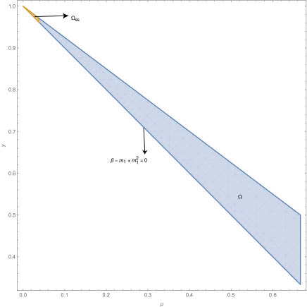
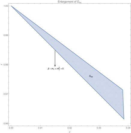
Figure 1: spaces $\Omega$ and $\Omega_{ss}$ of masses

Some tedious computation further yields the corresponding eigenvectors

$$\begin{array}[]{c}\mathcal{E}_{1}=\left(\frac{m_{1}-m_{3}}{\frac{\kappa m_{1}}{m_{3}}},\frac{3m_{2}-2\alpha-1}{\frac{\sqrt{3}\kappa m_{1}}{m_{3}}},\frac{m_{2}-\alpha-m_{1}}{\frac{\kappa m_{2}}{m_{3}}},\frac{\alpha+3m_{3}-1}{\frac{\sqrt{3}\kappa m_{2}}{m_{3}}},\frac{\alpha-m_{2}+m_{3}}{\kappa},\frac{\alpha+3m_{1}-1}{\sqrt{3}\kappa}\right)^{\top},\\[16.0pt] \mathcal{E}_{2}=\mathbf{i}\mathcal{E}_{1},\end{array}$$ (3.24)

where

$$\kappa=\sqrt{\frac{4\beta m_{3}\left(2-6\beta+\alpha-3\alpha m_{2}\right)}{3m_{1}m_{2}}},~{}~{}~{}~{}$$

$$\alpha=\sqrt{1-3\beta}.$$

4 Classical Results of Hamiltonian System

In this section, let us recall some necessary aspects of Hamiltonian system.

We consider an analytic Hamiltonian system, with $n$ degrees of freedom, having the origin as an equilibrium point:

$$H(p,q)=\sum_{j\geq 2}H_{j}(p,q),$$ (4.25)

where $H_{j}$ is a homogeneous polynomial of degree $j$ in $(p,q)$ for every $j\geq 2$.

Since we are interesting in stability, we confine ourself to the eigenvalues of the quadratic part $H_{2}$ of the Hamiltonian are all distinct and purely imaginary. Then in suitable symplectic coordinates, the quadratic part $H_{2}$ takes the form

$$H_{2}=\sum_{j=1}^{n}\frac{\omega_{j}(p_{j}^{2}+q_{j}^{2})}{2}.$$ (4.26)

Here every $\omega_{j}$ is called a characteristic frequency, and $\varpi=(\omega_{1},\cdots,\omega_{n})$ is called the frequency vector.

Definition 4.1

A frequency vector $\varpi$ satisfies a resonance relation of order $l>0$ if there exists a linear relationship

$$(k,\varpi)=k_{1}\omega_{1}+\cdots+k_{n}\omega_{n}=0,$$ (4.27)

where $k=(k_{1},\cdots,k_{n})\in\mathbb{Z}^{n}$ such that $|k|=|k_{1}|+\cdots+|k_{n}|=l$.

Definition 4.2

A frequency vector $\varpi$ is said to be $(c,\upsilon)$-Diophantine for some $c,\upsilon>0$ if we have

$$|(k,\varpi)|\geq\frac{c}{|k|^{\upsilon}},~{}~{}~{}~{}~{}~{}~{}~{}~{}\forall k\in\mathbb{Z}^{n}~{}such~{}that~{}~{}|k|\neq 0.$$

A $(c,\upsilon)$-Diophantine frequency vector $\varpi$ is also said to be strongly incommensurable.

Definition 4.3

A Birkhoff normal form of degree $l$ for the Hamiltonian (4.25) is a polynomial of degree $l$ in symplectic variables $x,y$ that is actually a polynomial of degree $[l/2]$ in the variables $\varrho_{j}=\frac{x_{j}^{2}+y_{j}^{2}}{2}$.

Given $l\geq 4$, assume that the frequency vector $\varpi$ is nonresonant up to order $l$. The well-known Birkhoff theorem [6] states that, in some neighbourhood of the origin, there exists a symplectic change of variables $(p,q)\mapsto(x,y)$, near to the identity map, such that in the new variables the Hamiltonian function is reduced to a Birkhoff normal form $\mathcal{H}_{Bl}(\varrho)$ of degree $l$ up to terms of degree higher than $l$:

$$H(p,q)=\mathcal{H}(x,y)=\mathcal{H}_{Bl}(\varrho)+O(|x|+|y|)^{l+1}.$$

Let us consider a nearly-integrable Hamiltonian written in action-angle variables $\varrho,\varphi$ defined by $x_{j}=\sqrt{2\varrho_{j}}\cos\varphi_{j},y_{j}=\sqrt{2\varrho_{j}}\sin\varphi_{j}$:

$$\mathcal{H}(\varrho,\varphi)=\mathcal{H}_{Bl}(\varrho)+\mathcal{R}_{l}(\varrho,\varphi),$$ (4.28)

where $\mathcal{R}(\varrho,\varphi)=O(\|\varrho\|)^{[l/2]+1}$, here $\|\varrho\|=\max_{1\leq j\leq n}|\varrho_{j}|$.

Let us recall the important concepts of non-degenerate and isoenergetically non-degenerate (see [3]):

Definition 4.4

The Hamiltonian system (4.25) or (4.28) is called to be non-degenerate in a neighbourhood of the origin if

$$det\left(\frac{\partial^{2}\mathcal{H}_{Bl}}{\partial\varrho^{2}}|_{\varrho=0}\right)\neq 0;$$

The Hamiltonian system (4.25) or (4.28) is called to be isoenergetically non-degenerate in a neighbourhood of the origin if

$$det\left(\begin{array}[]{cc}\frac{\partial^{2}\mathcal{H}_{Bl}}{\partial\varrho^{2}}|_{\varrho=0}&\varpi^{\top}\\ \varpi&0\\ \end{array}\right)\neq 0.$$

Then it is well known that:

Theorem 4.1

(KAM [4, 28]) In a neighbourhood of an equilibrium point, a non-degenerate or isoenergetically non-degenerate Hamiltonian with a nonresonant frequency vector up to order $4$ has invariant tori close to the tori of the linearized system. These tori form a set whose relative measure in the polydisc $\|\varrho\|<\epsilon$ tends to 1 as $\epsilon\rightarrow 0$. In an isoenergetically non-degenerate system such tori occupy a larger part of each energy level passing near the equilibrium position.

Furthermore, on the relative measure of the set of invariant tori in the polydisc $\|\varrho\|<\epsilon$ we have

Theorem 4.2

([33, 9]) Consider a non-degenerate or isoenergetically non-degenerate Hamiltonian in a neighbourhood of an equilibrium point. If the frequency vector $\varpi$ is nonresonant up to order $l\geq 4$, then the relative measure of the set of invariant tori in the polydisc $\|\varrho\|<\epsilon$ is at least $1-O(\epsilon^{\frac{l-3}{4}})$. If the frequency vector $\varpi$ satisfies the strong incommensurability condition, i.e., $(c,\upsilon)$-Diophantine condition, then this measure is $1-O(\exp(-\tilde{c}\epsilon^{\frac{-1}{\upsilon+1}}))$ for a positive number $\tilde{c}=const$.

Let us further consider effective stability of a nearly-integrable Hamiltonian

$$\mathcal{H}(\varrho,\varphi)=(\varrho,\varpi)+\mathcal{R}_{2}(\varrho,\varphi).$$ (4.29)

First, under $(c,\upsilon)$-Diophantine condition we have

Theorem 4.3

([15, 14, 16]) Assume the frequency vector $\varpi$ is $(c,\upsilon)$-Diophantine, then there exist $c_{1},c_{2},c_{3}=const>0$ such that for every orbit $(\varrho(t),\varphi(t))$ of (4.29), with $\|\varrho(0)\|<\epsilon$, one has

$$\|\varrho(t)-\varrho(0)\|\leq c_{1}\epsilon^{3}~{}~{}~{}~{}~{}~{}~{}~{}~{}~{}~{}~{}~{}~{}for~{}~{}~{}|t|\leq c_{3}\exp(c_{2}\epsilon^{\frac{-1}{\upsilon+1}}),$$

provided $\epsilon$ is sufficiently small.

Although all of the $(c,\upsilon)$-Diophantine frequency vectors are abundant in measure, however, non-Diophantine frequency vectors form a dense open set in the space of frequency vectors. Therefore, Diophantine frequency vectors could be quite exceptional in some sense.

Definition 4.5

([31]) Let $h$ be a real analytic in the vicinity of the closed ball $\overline{B_{r}}$ of radius $r>0$ in $\mathbb{R}^{n}$ and has no critical points in $\overline{B_{r}}$. Then $h$ is steep if and only if its restriction $h|_{\mathcal{P}}$ to any proper affine subspace $\mathcal{P}\subset\mathbb{R}^{n}$ admits only isolated critical points.

Definition 4.6

Let $h$ be a polynomial of degree $l$ in $\varrho_{1},\cdots,\varrho_{n}$ such that

$$h(\varrho)=h_{1}(\varrho)+\cdots h_{l}(\varrho),$$

where is $h_{j}(\varrho)$ a homogeneous polynomial of degree $k$ in $\varrho_{1},\cdots,\varrho_{n}$. We say that the function $h$ is

• convex at $\varrho=0$, if the quadratic form $h_{2}(\varrho)$ is either positive or negative definite;

• quasi-convex at $\varrho=0$, if

  $$h_{1}(\varrho)=0,h_{2}(\varrho)=0~{}~{}~{}~{}~{}~{}~{}~{}~{}\Rightarrow~{}~{}~{}~{}~{}~{}~{}~{}~{}\varrho=0;$$

• directionally quasi-convex at $\varrho=0$, if

  $$h_{1}(\varrho)=0,h_{2}(\varrho)=0,\varrho_{1},\cdots,\varrho_{n}\geq 0~{}~{}~{}~{}~{}~{}\Rightarrow~{}~{}~{}~{}~{}~{}\varrho=0.$$

Theorem 4.4

([5, 11, 30, 34]) Consider the Hamiltonian (4.28) in a neighbourhood of the origin $\varrho=0$. Assume the frequency vector $\varpi$ is nonresonant up to order $l\geq 4$ and the unperturbed Hamiltonian $\mathcal{H}_{Bl}$ is a (directionally) quasi-convex function, then there exist two positive constants $a,b$ such that, for sufficiently small $\epsilon$, any orbit $(\varrho(t),\varphi(t))$ of (4.28), with $\|\varrho(0)\|<\epsilon$, satisfies

$$\|\varrho(t)-\varrho(0)\|\leq c_{1}\epsilon^{a}~{}~{}~{}~{}~{}~{}~{}~{}~{}~{}~{}~{}~{}~{}for~{}~{}~{}|t|\leq c_{3}\exp(c_{2}\epsilon^{-b}),$$

here $c_{1},c_{2},c_{3}=const>0$.

Remark 4.1

Two positive constants $a,b$ in Theorem 4.4 can be chosen as $a=\frac{1+\sigma}{n+\sigma},b=\frac{1}{n+\sigma}$ for any $\sigma\geq 0$, for instance, $a=\frac{1}{n},b=\frac{1}{n}$ or $a=\frac{1}{2},b=\frac{1}{2n}$. It should be no surprise that two constants $a,b$ in Theorem 4.4 are worse than that in Theorem 4.3.

Remark 4.2

Note that there are some differences between Theorem 4.4 and the celebrated Nekhoroshev theorem [29]. In his celebrated 1977 article [29], Nekhoroshev conjectured that, if the function $\mathcal{H}_{Bl}$ is steep, a weaker condition than convex or quasi-convex properties, the Theorem 4.4 is also correct, however, this conjecture is not complete answered up to now. Note that directionally quasi-convex function may be not steep.

5 The Birkhoff Normal Form

To discuss the stability of relative equilibria, it would be better to employ Hamiltonian form of the $N$-body problem.

5.1 The Hamiltonian Near Relative Equilibria

It is easy to see that the system (3.16) is essentially a Lagrangian system with the Lagrangian function

$$\mathcal{L}_{\mathcal{J}}(z,r,\dot{z},\dot{r})=\frac{\dot{r}^{2}}{2}+\frac{(1+r)^{2}}{2}\left[\dot{z}^{2}_{0}+|\dot{z}|^{2}-\left(\dot{z}^{\top}Q{z}-\frac{\mathcal{J}}{(1+r)^{2}}\right)^{2}\right]+\frac{U(z)}{1+r}.$$

Recall that we have assumed that $\rho=1$.

It follows from the Legendre Transform that the corresponding Hamiltonian is

$$H(r,z,s,w) = s\dot{r}+w^{\top}\dot{r}-\mathcal{L}_{\mathcal{J}}(z,r,\dot{z},\dot{r})$$

$$= \frac{s^{2}}{2}+\frac{(1+r)^{2}}{2}[\dot{z}^{2}_{0}+|\dot{z}|^{2}+\frac{\mathcal{J}^{2}}{(1+r)^{4}}-(\dot{z}^{\top}Q{z})^{2}]-\frac{U(z)}{1+r},$$

where

$$\begin{array}[]{lr}s=\frac{\partial{\mathcal{L}_{\mathcal{J}}}}{\partial\dot{r}}=\dot{r},\\ w_{k}=\frac{\partial{\mathcal{L}_{\mathcal{J}}}}{\partial\dot{z}_{k}}=(1+r)^{2}\left[\frac{\dot{z}^{\top}z}{z^{2}_{0}}z_{k}+\dot{z}_{k}+\sum_{j=1}^{2N-4}q_{kj}{z}_{j}(\frac{\mathcal{J}}{(1+r)^{2}}-\dot{z}^{\top}Qz)\right].\end{array}$$

Moreover, a straightforward computation shows that:

$$\begin{array}[]{c}\dot{z}^{2}_{0}=\frac{(\dot{z}^{\top}z)^{2}}{z^{2}_{0}}=(\frac{z^{\top}w}{(1+r)^{2}})^{2}+O(\parallel(z,w)\parallel^{6}),\\[8.0pt] \dot{z}_{k}=\frac{w_{k}-\mathcal{J}\sum_{j=1}^{2N-4}q_{kj}{z}_{j}}{(1+r)^{2}}-\frac{\dot{z}^{\top}z}{z^{2}_{0}}z_{k}+\dot{z}^{\top}Q{z}\sum_{j=1}^{2N-4}q_{kj}{z}_{j}\\ =\frac{w_{k}-\mathcal{J}\sum_{j=1}^{2N-4}q_{kj}{z}_{j}}{(1+r)^{2}}-\frac{z^{\top}w}{(1+r)^{2}}z_{k}+\sum_{j=1}^{2N-4}q_{kj}{z}_{j}(\frac{w^{\top}Q{z}-\mathcal{J}{|z|}^{2}}{(1+r)^{2}})+O(\parallel(z,w)\parallel^{5}).\end{array}$$

As a result, we have

$$\begin{array}[]{l}H(r,z,s,w)=\frac{s^{2}}{2}+\frac{1}{2(1+r)^{2}}[\mathcal{J}^{2}+\sum_{k=1}^{2N-4}(w_{k}-\mathcal{J}\sum_{j=1}^{2N-4}q_{kj}{z}_{j})^{2}+(w^{\top}Q{z}-\mathcal{J}{|z|}^{2})^{2}\\[6.0pt] ~{}~{}~{}~{}~{}~{}~{}~{}~{}~{}~{}~{}~{}~{}~{}~{}~{}~{}-~{}(z^{\top}w)^{2}+O(\parallel(z,w)\parallel^{6})]-\frac{U(z)}{1+r}\\[10.0pt] =\frac{\omega^{2}}{2}-\omega^{2}r+\frac{s^{2}+3\omega^{2}r^{2}+|w|^{2}-2\omega w^{\top}Q{z}+\omega^{2}|z|^{2}}{2}-{r(2\omega^{2}r^{2}+|w|^{2}-2\omega w^{\top}Q{z}+\omega^{2}|z|^{2})}\\[6.0pt] +\frac{5\omega^{2}r^{4}+3r^{2}(|w|^{2}-2\omega w^{\top}Q{z}+\omega^{2}|z|^{2})}{2}+\frac{(w^{\top}Q{z}-\mathcal{J}{|z|}^{2})^{2}-(z^{\top}w)^{2}}{2}+O(\parallel(r,z,w)\parallel^{5})-\frac{U(z)}{1+r}.\end{array}$$ (5.30)

We remark that the relative equilibrium $\rho e^{\mathbf{i}\omega t}\mathbf{r}_{0}$ is just reduced to the origin, an equilibrium point, of an analytic Hamiltonian system with Hamiltonian (5.30).

5.2 The Hamiltonian Near Lagrange Triangular Point

For the three-body problem, let us further compute the Hamiltonian $H(r,z,s,w)$ near Lagrange triangular point $\mathbf{r}_{0}$ in (3.20). As a matter of notational convenience, set

$$q_{0}=r,q_{1}=z_{1},q_{2}=z_{2},p_{0}=s,p_{1}=w_{1},p_{2}=w_{2}.$$

First, by (3.24), some tedious computation yields that

$$U(z)=\mathcal{U}(z_{0}\hat{\mathbf{r}}_{0}+{z_{1}\hat{\mathcal{E}}_{1}}+{z_{2}\hat{\mathcal{E}}_{2}})=\widetilde{\mathcal{U}}(z_{0}\hat{\mathbf{r}}_{0}+{z_{1}\hat{\mathcal{E}}_{1}}+{z_{2}\hat{\mathcal{E}}_{2}})$$

$$=\lambda+\frac{1}{2}(\lambda_{1}q_{1}^{2}+\lambda_{2}q_{2}^{2})+a_{30}q_{1}^{3}+a_{12}q_{1}q_{2}^{2}+a_{21}q_{1}^{2}q_{2}+a_{03}q_{2}^{3}$$

$$+a_{40}q_{1}^{4}+a_{13}q_{1}q_{2}^{3}+a_{22}q_{1}^{2}q_{2}^{2}+a_{31}q_{1}^{3}q_{2}+a_{04}q_{2}^{4}+\cdots,$$

where $\cdots$ denotes the terms of degree higher than 4, and

$$\begin{array}[]{lr}a_{30}=(13\alpha+5)a_{3012},\\ a_{12}=-3(9\alpha+5)a_{3012},\\ a_{3012}=\frac{m_{3}\beta^{3}(\alpha-1)^{2}\left(\alpha-3m_{1}+1\right)\left[3\alpha(2\alpha-1)+(2-5\alpha)\left(m_{2}-m_{3}\right)+3m_{1}\left(3\alpha-2m_{2}+2m_{3}\right)\right]}{36\sqrt{3}\kappa^{3}m_{1}^{2}m_{2}^{2}};\end{array}$$

$$\begin{array}[]{lr}a_{21}=-3(9\alpha-5)a_{2103},\\ a_{03}=(13\alpha-5)a_{2103},\\ a_{2103}=-\frac{m_{3}\beta^{3}(\alpha+1)^{2}\left(\alpha+3m_{1}-1\right)\left[10\alpha^{2}+\alpha-9\alpha m_{2}+9\alpha m_{3}-3(\alpha-4)m_{1}-18m_{1}^{2}-2\right]}{108\kappa^{3}m_{1}^{2}m_{2}^{2}};\end{array}$$

$$\begin{array}[]{lr}a_{40}=\left[-\left(\alpha^{2}-1\right)^{2}\left(40\alpha^{3}-123\alpha^{2}+35\right)-27\left(41\alpha^{4}+8\alpha^{3}+50\alpha^{2}-35\right)m_{1}m_{2}m_{3}\right]a_{4004},\\ a_{04}=\left[\left(\alpha^{2}-1\right)^{2}\left(40\alpha^{3}+123\alpha^{2}-35\right)-27\left(41\alpha^{4}-8\alpha^{3}+50\alpha^{2}-35\right)m_{1}m_{2}m_{3}\right]a_{4004},\\ a_{4004}=\frac{\left[m_{1}\left(8-13\alpha^{2}-4\alpha+3(4\alpha-1)\left(m_{2}-m_{3}\right)\right)+(\alpha-1)\left(1-8\alpha^{2}+\alpha+(7\alpha-1)\left(m_{2}-m_{3}\right)\right)+3(4\alpha-7)m_{1}^{2}+18m_{1}^{3}\right]}{1296\kappa^{4}m_{1}^{3}m_{2}^{4}/(\beta^{7/2}m_{3})};\end{array}$$

$$\begin{array}[]{c}a_{22}=\frac{a_{4004}\left[(297\beta-64)+\frac{3\left(297\beta^{2}-527\beta+96\right)m_{1}}{\beta}+\frac{\left(-1485\beta^{2}+2504\beta-448\right)m_{1}^{2}}{\beta^{2}}+\frac{\left(891\beta^{2}-1284\beta+224\right)m_{1}^{3}\left(2\beta+\left(1-m_{1}\right){}^{2}\right)}{\beta^{3}}\right]}{m_{2}m_{3}/(54\beta^{3})};\end{array}$$

$$\begin{array}[]{lr}a_{13}=-a_{31}=\frac{\left[\beta+m_{3}(3m_{3}-2)\right]\left(\alpha+3m_{1}-1\right)\left[8\alpha^{2}-\alpha-7\alpha\left(m_{2}-m_{3}\right)+m_{1}\left(3\alpha-3\left(m_{2}-m_{3}\right)+6\right)-9m_{1}^{2}+\left(m_{2}-m_{3}\right)-1\right]}{4\sqrt{3}\kappa^{4}m_{1}^{3}m_{2}^{3}/(35\beta^{11/2}m_{3})}.\end{array}$$

It follows that the Hamiltonian (5.30) becomes

$$H=-\frac{\omega_{0}^{2}}{2}+H_{2}+H_{3}+H_{4}+\cdots,$$ (5.31)

where

$$\begin{array}[]{lr}\omega_{0}=\omega=\beta^{3/4},\\ H_{2}=\frac{1}{2}[p_{0}^{2}+p_{1}^{2}+p_{2}^{2}+2\omega_{0}\left(p_{1}q_{2}-p_{2}q_{1}\right)+\omega_{0}^{2}(q_{0}^{2}+\frac{(3\alpha-1)}{2}q_{1}^{2}-\frac{(3\alpha+1)}{2}q_{2}^{2})],\\ \begin{aligned} &H_{3}=2\omega_{0}p_{2}q_{1}q_{0}-2\omega_{0}p_{1}q_{2}q_{0}-p_{2}^{2}q_{0}-p_{1}^{2}q_{0}-\omega_{0}^{2}q_{0}^{3}-a_{03}q_{2}^{3}\\ &-a_{12}q_{1}q_{2}^{2}-a_{21}q_{1}^{2}q_{2}-a_{30}q_{1}^{3}-\frac{\omega_{0}^{2}}{4}q_{0}\left((3\alpha+1)q_{1}^{2}+(1-3\alpha)q_{2}^{2}\right),\end{aligned}\\ \begin{aligned} &H_{4}=\frac{3}{2}p_{1}^{2}q_{0}^{2}+\frac{3}{2}p_{2}^{2}q_{0}^{2}-\frac{1}{2}p_{1}^{2}q_{1}^{2}+\frac{1}{2}p_{2}^{2}q_{1}^{2}+\frac{1}{2}p_{1}^{2}q_{2}^{2}-\frac{1}{2}p_{2}^{2}q_{2}^{2}-3\omega_{0}p_{2}q_{1}q_{0}^{2}+3\omega_{0}p_{1}q_{2}q_{0}^{2}\\ &-\omega_{0}p_{2}q_{1}^{3}+\omega_{0}p_{1}q_{2}^{3}-\omega_{0}p_{2}q_{1}q_{2}^{2}+\omega_{0}p_{1}q_{1}^{2}q_{2}+\omega_{0}^{2}\frac{3}{2}q_{0}^{4}-2p_{1}p_{2}q_{2}q_{1}+a_{21}q_{0}q_{2}q_{1}^{2}\\ &+a_{30}q_{0}q_{1}^{3}-a_{31}q_{2}q_{1}^{3}+a_{12}q_{0}q_{2}^{3}+a_{03}q_{0}q_{1}q_{2}^{2}-a_{13}q_{1}q_{2}^{3}+(\frac{\omega_{0}^{2}}{2}-a_{04})q_{2}^{4}+(\frac{\omega_{0}^{2}}{2}-a_{40})q_{1}^{4}\\ &+(\omega_{0}^{2}-a_{22})q_{1}^{2}q_{2}^{2}+\frac{3\omega_{0}^{2}}{4}q_{0}^{2}\left((\alpha+1)q_{1}^{2}-(\alpha-1)q_{2}^{2}\right).\end{aligned}\end{array}$$

Note that, without loss of generality, we will sometimes omit the constant term $-\frac{\omega^{2}}{2}$ in (5.31) in the following content.

Our task now is to look for a change of variables from $(p,q)$ to $(x,y)$ such that $H_{2}$ takes the form

$$\frac{\omega_{0}(x_{0}^{2}+y_{0}^{2})}{2}-\frac{\omega_{1}(x_{1}^{2}+y_{1}^{2})}{2}+\frac{\omega_{2}(x_{2}^{2}+y_{2}^{2})}{2}.$$

Let $\mathbb{J}$ denote the usual symplectic matrix $\left(\begin{array}[]{cc}&-\mathbb{I}\\ \mathbb{I}&\\ \end{array}\right)$. A straight forward computation shows that the eigenvalues of the matrix $\mathbb{J}\frac{\partial^{2}H_{2}}{\partial^{2}(p,q)}$ are

$$\pm\omega_{0}\mathbf{i},~{}~{}~{}~{}\pm\omega_{1}\mathbf{i},~{}~{}~{}~{}\pm\omega_{2}\mathbf{i},~{}~{}~{}~{}~{}~{}~{}~{}$$

where

$$\begin{array}[]{lr}\omega_{1}=\mu_{1}\omega_{0},~{}~{}~{}~{}~{}~{}~{}~{}~{}~{}~{}~{}\mu_{1}=\sqrt{\frac{{1-\sqrt{1-27\beta}}}{{2}}},\\ \omega_{2}=\mu_{2}\omega_{0},~{}~{}~{}~{}~{}~{}~{}~{}~{}~{}~{}~{}\mu_{2}=\sqrt{\frac{{1+\sqrt{1-27\beta}}}{{2}}}.\end{array}~{}~{}~{}~{}$$

Note that we can restrict our attention to the variables $p_{1},p_{2},q_{1},q_{2}$. For the eigenvalues $\omega_{1}\mathbf{i},\omega_{2}\mathbf{i}$, the corresponding eigenvectors are

$$\begin{array}[]{c}\left(\frac{3\alpha-\gamma}{4}\beta^{3/4},\frac{\mathbf{i}\left(3\alpha+\gamma\right)\omega_{1}}{3\alpha+\gamma-4},\frac{4\mathbf{i}\omega_{1}\beta^{-3/4}}{3\alpha+\gamma-4},1\right)^{\top}~{}~{}~{}\text{and}~{}~{}~{}\left(\frac{3\alpha+\gamma}{4}\beta^{3/4},\frac{\mathbf{i}\left(\gamma-3\alpha\right)\omega_{2}}{-3\alpha+\gamma+4},-\frac{4\mathbf{i}\omega_{2}\beta^{-3/4}}{-3\alpha+\gamma+4},1\right)^{\top},\end{array}$$

where

$$\gamma=\sqrt{1-27\beta}.$$

It follows that we can introduce the following symplectic transformation to reduce the Hamiltonian:

$$\left\{\begin{array}[]{lr}p_{0}=\sqrt{\omega}x_{0}&\\ q_{0}=\frac{y_{0}}{\sqrt{\omega}}&\\ p_{1}=\frac{\omega_{0}(3\alpha-\gamma)}{4\sqrt{\frac{2\gamma\omega_{1}}{4-3\alpha-\gamma}}}x_{1}+\frac{\omega_{0}(3\alpha+\gamma)}{4\sqrt{\frac{2\gamma\omega_{2}}{4-3\alpha+\gamma}}}y_{2}&\\ p_{2}=\frac{(\gamma-3\alpha)\sqrt{\frac{\gamma\omega_{2}}{-3\alpha+\gamma+4}}}{\sqrt{2}\gamma}x_{2}-\frac{(3\alpha+\gamma)\sqrt{\frac{\gamma\omega_{1}}{-3\alpha-\gamma+4}}}{\sqrt{2}\gamma}y_{1}&\\ q_{1}=-\frac{2\sqrt{2}\sqrt{\frac{\gamma\omega_{2}}{-3\alpha+\gamma+4}}}{\gamma\omega_{0}}x_{2}-\frac{2\sqrt{2}\sqrt{\frac{\gamma\omega_{1}}{-3\alpha-\gamma+4}}}{\gamma\omega_{0}}y_{1}&\\ q_{2}=\frac{1}{\sqrt{2}\sqrt{\frac{\gamma\omega_{1}}{-3\alpha-\gamma+4}}}x_{1}+\frac{1}{\sqrt{2}\sqrt{\frac{\gamma\omega_{2}}{-3\alpha+\gamma+4}}}y_{2}&\end{array}\right.$$ (5.32)

In fact, by the transformation (5.32), it follows that the Hamiltonian (5.31) becomes

$$H(x,y)=\frac{\omega_{0}(x_{0}^{2}+y_{0}^{2})}{2}-\frac{\omega_{1}(x_{1}^{2}+y_{1}^{2})}{2}+\frac{\omega_{2}(x_{2}^{2}+y_{2}^{2})}{2}+H_{3}(x,y)+H_{4}(x,y)+\cdots.$$

But we’d better introduce the following complex symplectic transformation to reduce the Hamiltonian:

$$\left\{\begin{array}[]{lr}x_{0}=\frac{\zeta_{0}}{\sqrt{2}}+\frac{\textbf{i}\eta_{0}}{\sqrt{2}}&\\ y_{0}=\frac{\eta_{0}}{\sqrt{2}}+\frac{\textbf{i}\zeta_{0}}{\sqrt{2}}&\\ x_{1}=\frac{\zeta_{1}}{\sqrt{2}}+\frac{\textbf{i}\eta_{1}}{\sqrt{2}}&\\ y_{1}=\frac{\eta_{1}}{\sqrt{2}}+\frac{\textbf{i}\zeta_{1}}{\sqrt{2}}&\\ x_{2}=\frac{\zeta_{2}}{\sqrt{2}}+\frac{\textbf{i}\eta_{2}}{\sqrt{2}}&\\ y_{2}=\frac{\eta_{2}}{\sqrt{2}}+\frac{\textbf{i}\zeta_{2}}{\sqrt{2}}&\end{array}\right.$$ (5.33)

Then, by the transformation (5.33), it follows that the Hamiltonian (5.31) becomes

$$H(\zeta,\eta)=\textbf{i}\omega_{0}\zeta_{0}\eta_{0}-\textbf{i}\omega_{1}\zeta_{1}\eta_{1}+\textbf{i}\omega_{2}\zeta_{2}\eta_{2}+H_{3}(\zeta,\eta)+H_{4}(\zeta,\eta)+\cdots.$$

Note that a formal series

$$f=\sum_{k,l}f_{k,l}\zeta^{k}\eta^{l},~{}~{}~{}~{}~{}~{}~{}~{}k,l\in\mathbb{N}^{3}$$

in the variables $(\zeta,\eta)\in\mathbb{C}^{6}$ represents a real formal series in the variables $(x,y)$ if and only if

$$f_{k,l}=\textbf{i}^{|k+l|}\overline{f_{l,k}}.$$

We will further perform a change of variables $(\zeta,\eta)\mapsto(u,v)$ with a generating function

$$u_{0}\eta_{0}+u_{1}\eta_{1}+u_{2}\eta_{2}+S_{3}(u,\eta)+S_{4}(u,\eta)+\cdots,$$

such that in the new variables $(u,v)$ the Hamiltonian function reduces to a Birkhoff normal form of degree 4 up to terms of degree higher than 4:

$$H(\zeta,\eta)=H(\zeta(u,v),\eta(u,v))=\mathcal{H}(u,v)$$ (5.34)

$$=\textbf{i}\omega_{0}u_{0}v_{0}-\textbf{i}\omega_{1}u_{1}v_{1}+\textbf{i}\omega_{2}u_{2}v_{2}-\frac{1}{2}[\omega_{00}(u_{0}v_{0})^{2}+\omega_{11}(u_{1}v_{1})^{2}+\omega_{22}(u_{2}v_{2})^{2}$$

$$+2\omega_{01}(u_{0}v_{0}u_{1}v_{1})+2\omega_{02}(u_{0}v_{0}u_{2}v_{2})+2\omega_{12}(u_{1}v_{1}u_{2}v_{2})]+\cdots,$$

where $S_{3}$ and $S_{4}$ are forms of degree 3 and 4 in $u,\eta$, and

$$\zeta=u+\frac{\partial S_{3}}{\partial\eta}+\frac{\partial S_{4}}{\partial\eta}+\cdots,~{}~{}~{}~{}~{}~{}~{}~{}~{}~{}~{}~{}v=\eta+\frac{\partial S_{3}}{\partial u}+\frac{\partial S_{4}}{\partial u}+\cdots.$$

First of all, it is easy to see that $\beta=\frac{1}{27}$ yields that frequency vector $\varpi=(\omega_{0},-\omega_{1},\omega_{2})$ satisfies a resonance relations of order 2; and all of resonance relations of order 3 or 4 satisfied by $\varpi$ are

$$\left\{\begin{array}[]{lr}\omega_{0}-2\omega_{1}=0~{}~{}~{}~{}~{}~{}iff~{}~{}~{}\beta=\frac{1}{36},&\\ \omega_{2}-2\omega_{1}=0~{}~{}~{}~{}~{}~{}iff~{}~{}~{}\beta=\frac{16}{675},&\\ \omega_{0}-3\omega_{1}=0~{}~{}~{}~{}~{}~{}iff~{}~{}~{}\beta=\frac{32}{2187},&\\ \omega_{0}+\omega_{1}-2\omega_{2}=0~{}~{}~{}~{}~{}~{}iff~{}~{}~{}\beta=\frac{64}{1875},&\\ \omega_{2}-3\omega_{1}=0~{}~{}~{}~{}~{}~{}iff~{}~{}~{}\beta=\frac{1}{75}.&\end{array}\right.$$ (5.35)

For other values of $\beta$, we make use of the relation

$$H(u+\frac{\partial S_{3}}{\partial\eta}+\frac{\partial S_{4}}{\partial\eta}+\cdots,\eta)=\mathcal{H}(u,\eta+\frac{\partial S_{3}}{\partial u}+\frac{\partial S_{4}}{\partial u}+\cdots)$$ (5.36)

to find the Birkhoff normal form of degree 4.

Equating the forms of order 3 in $u,\eta$ of (5.36) we obtain

$$\textbf{i}\omega_{0}(\frac{\partial S_{3}}{\partial\eta_{0}}\eta_{0}-\frac{\partial S_{3}}{\partial u_{0}}u_{0})-\textbf{i}\omega_{1}(\frac{\partial S_{3}}{\partial\eta_{1}}\eta_{1}-\frac{\partial S_{3}}{\partial u_{1}}u_{1})+\textbf{i}\omega_{2}(\frac{\partial S_{3}}{\partial\eta_{2}}\eta_{2}-\frac{\partial S_{3}}{\partial u_{2}}u_{2})+H_{3}(u,\eta)=0.$$ (5.37)

It follows that $S_{3}$ can be determined.

Then by equating the forms of order 4 in $u,\eta$ of (5.36) we obtain

$$\textbf{i}\omega_{0}(\frac{\partial S_{4}}{\partial\eta_{0}}\eta_{0}-\frac{\partial S_{4}}{\partial u_{0}}u_{0})-\textbf{i}\omega_{1}(\frac{\partial S_{4}}{\partial\eta_{1}}\eta_{1}-\frac{\partial S_{4}}{\partial u_{1}}u_{1})+\textbf{i}\omega_{2}(\frac{\partial S_{4}}{\partial\eta_{2}}\eta_{2}-\frac{\partial S_{4}}{\partial u_{2}}u_{2})+H_{3\rightarrow 4}+H_{4}(u,\eta)$$

$$+\frac{1}{2}[\omega_{00}(u_{0}v_{0})^{2}+\omega_{11}(u_{1}v_{1})^{2}+\omega_{22}(u_{2}v_{2})^{2}+2\omega_{01}(u_{0}v_{0}u_{1}v_{1})+2\omega_{02}(u_{0}v_{0}u_{2}v_{2})$$

$$+2\omega_{12}(u_{1}v_{1}u_{2}v_{2})]=0,$$

where $H_{3\rightarrow 4}$ is the forms of order 4 of $H_{3}(u+\frac{\partial S_{3}}{\partial\eta},\eta)$. It follows that $S_{4}$ and the Birkhoff normal form of degree 4 in (5.34) can be determined.

By switching to action-angle variables, the obtained Birkhoff normal form in (5.34) becomes

$$\mathcal{H}_{B4}=\omega_{0}\varrho_{0}-\omega_{1}\varrho_{1}+\omega_{2}\varrho_{2}+\frac{1}{2}[\omega_{00}\varrho_{0}^{2}+\omega_{11}\varrho_{1}^{2}+\omega_{22}\varrho_{2}^{2}$$ (5.38)

$$+2\omega_{01}\varrho_{0}\varrho_{1}+2\omega_{02}\varrho_{0}\varrho_{2}+2\omega_{12}\varrho_{1}\varrho_{2}],$$

where $\varrho_{j}=\textbf{i}u_{j}v_{j}$ ($j=0,1,2$) are action variables, and

$$\begin{array}[]{c}\omega_{00}=-3,\\ \omega_{01}=-\frac{\sqrt{\gamma+1}\left(21\gamma^{3}-40\gamma^{2}+15\gamma+4\right)}{12\sqrt{6}\sqrt{\beta}\gamma(2\gamma-1)},\\ \omega_{02}=-\frac{\sqrt{\gamma+1}\left(21\gamma^{2}+19\gamma-4\right)}{4\sqrt{2}\gamma(2\gamma+1)},\end{array}$$

$$\begin{array}[]{c}\omega_{11}=\frac{(\gamma-1)\left(1211\gamma^{4}-1336\gamma^{3}+279\gamma^{2}+158\gamma-76\right)}{72\gamma^{2}\left(10\gamma^{2}-11\gamma+3\right)}-\frac{3\beta^{3}\left(31\gamma^{2}+286\gamma-236\right)}{8(\gamma-1)\gamma^{2}(5\gamma-3)m_{1}m_{2}m_{3}},\\ \omega_{22}=-\frac{(\gamma+1)\left(1211\gamma^{4}+1336\gamma^{3}+279\gamma^{2}-158\gamma-76\right)}{72\gamma^{2}\left(10\gamma^{2}+11\gamma+3\right)}-\frac{3\beta^{3}\left(31\gamma^{2}-286\gamma-236\right)}{8\gamma^{2}(\gamma+1)(5\gamma+3)m_{1}m_{2}m_{3}},\end{array}$$

$$\begin{array}[]{c}\begin{aligned} &\omega_{12}=\frac{\sqrt{3\beta}}{4(18225\beta^{2}-1107\beta+16)m_{1}m_{2}m_{3}}[(360855\beta^{2}-32265\beta+624)m_{1}^{3}+\\ &(-360855\beta^{2}+32265\beta-624)m_{1}^{2}+3\beta(120285\beta^{2}-10755\beta+208)m_{1}-4\beta^{2}(432\beta+43)].\end{aligned}\end{array}$$

We remark that

Theorem 5.1

The set $\Gamma_{r}$ of $\beta\in(0,\frac{1}{27})$ corresponding to resonant frequency vectors $\varpi=(\omega_{0},-\omega_{1},\omega_{2})$ is countable and dense. The set $\Gamma_{d}$ of $\beta\in(0,\frac{1}{27})$ corresponding to $(c,\upsilon)$-Diophantine frequency vectors $\varpi=(\omega_{0},-\omega_{1},\omega_{2})$ is a set of full measure for $\upsilon>6$.

Proof. First, it is easy to see that $\Gamma_{r}$ is countable.

Let us recall that

$$\begin{array}[]{lr}\omega_{0}=\beta^{3/4},~{}~{}~{}~{}\omega_{1}=\mu_{1}\omega_{0},~{}~{}~{}~{}\omega_{2}=\mu_{2}\omega_{0},\\ \mu_{1}=\sqrt{\frac{{1-\sqrt{1-27\beta}}}{{2}}},~{}~{}~{}~{}~{}~{}~{}~{}\mu_{2}=\sqrt{\frac{{1+\sqrt{1-27\beta}}}{{2}}}.\end{array}~{}~{}~{}~{}$$

Set

$$\Gamma_{0}=\{\varpi=(\omega_{0},-\omega_{1},\omega_{2}):\beta\in(0,\frac{1}{27})\},$$

$$\Gamma_{1}=\{(1,-\mu_{1},\mu_{2}):\beta\in(0,\frac{1}{27})\},$$

$$\Gamma_{2}=\{(\mu_{1},\mu_{2}):\beta\in(0,\frac{1}{27})\}.$$

Due to

$$\mu_{1}^{2}+\mu_{2}^{2}=1,$$

geometrically $\Gamma_{1},\Gamma_{2}$ are circular arcs. We parameterize $\Gamma_{2}$ as

$$\mu_{1}=\cos\vartheta,\mu_{2}=\sin\vartheta,~{}~{}~{}~{}~{}~{}~{}~{}\vartheta\in(\frac{\pi}{4},\frac{\pi}{2}).$$

Then the following mappings are diffeomorphisms:

$$\begin{array}[]{ccccccccc}(0,\frac{1}{27})&\rightarrow&\Gamma_{0}&\rightarrow&\Gamma_{1}&\rightarrow&\Gamma_{2}&\rightarrow&(\frac{\pi}{4},\frac{\pi}{2}):\\ \beta&\mapsto&\varpi&\mapsto&(1,-\mu_{1},\mu_{2})&\mapsto&(\mu_{1},\mu_{2})&\mapsto&\vartheta.\end{array}$$

Let us consider resonance relations

$$k_{0}-k_{1}\mu_{1}+k_{2}\mu_{2}=0.$$

Even if we consider only the case $k_{0}=0$, it is easy to see that the points in $\Gamma_{2}$ satisfying the relation

$$-k_{1}\mu_{1}+k_{2}\mu_{2}=0$$

are dense in $\Gamma_{2}$. Therefore it follows from the diffeomorphisms above that $\Gamma_{r}$ is also dense in the interval $(0,\frac{1}{27})$.

For fixed $k=(k_{0},k_{1},k_{2})\in\mathbb{Z}^{3},c$ and $\upsilon$ such that $|k|>0,0<c<1,\upsilon>6$, let us consider the inequality

$$|k_{0}-k_{1}\cos\vartheta+k_{2}\sin\vartheta|<\frac{c}{|k|^{\upsilon}}.$$

First, it is easy to see that

$$k_{1}^{2}+k_{2}^{2}>0.$$

Set

$$k_{1}=-\sqrt{k_{1}^{2}+k_{2}^{2}}\sin\vartheta_{0},~{}~{}~{}~{}~{}~{}~{}~{}k_{2}=\sqrt{k_{1}^{2}+k_{2}^{2}}\cos\vartheta_{0}.$$

Then we have

$$\frac{-k_{0}-\frac{c}{|k|^{\upsilon}}}{\sqrt{k_{1}^{2}+k_{2}^{2}}}<\sin(\vartheta+\vartheta_{0})<\frac{-k_{0}+\frac{c}{|k|^{\upsilon}}}{\sqrt{k_{1}^{2}+k_{2}^{2}}}.$$

But it is easy to show that, for any $\delta>0$, the measure of the set

$$\{x\in[-2\pi,2\pi]:y-\delta<\sin x<y+\delta\}$$

does not exceed $\sigma\sqrt{\delta}$, here $\sigma$ is a constant number. Hence the measure of the set of $\vartheta$ such that

$$|k_{0}-k_{1}\cos\vartheta+k_{2}\sin\vartheta|<\frac{c}{|k|^{\upsilon}}$$

does not exceed $\frac{\sigma\sqrt{c}}{\sqrt[4]{k_{1}^{2}+k_{2}^{2}}|k|^{\frac{\upsilon}{2}}}(\leq\frac{\sigma\sqrt{c}}{|k|^{\frac{\upsilon}{2}}})$.

Since the number of values of $k$ with $|k|=n$ does not exceed $25n^{2}$, the measure of the set $\Gamma_{c,\upsilon}\subset(\frac{\pi}{4},\frac{\pi}{2})$ of $\vartheta$ such that

$$|k_{0}-k_{1}\cos\vartheta+k_{2}\sin\vartheta|<\frac{c}{|k|^{\upsilon}}$$

for any $|k|>0$ does not exceed

$$\sum^{\infty}_{n=1}\frac{25\sigma\sqrt{c}n^{2}}{n^{\frac{\upsilon}{2}}}\leq 25\sigma\sqrt{c}\sigma_{\upsilon},$$

here the constant $\sigma_{\upsilon}$ depends only on $\upsilon$. As $c\rightarrow 0$, the measure of the set $\Gamma_{c,\upsilon}$ tends to zero. Therefore it follows from the diffeomorphisms above that the measure of the set $(0,\frac{1}{27})\setminus\Gamma_{d}$ is zero.

The proof of the theorem is now complete.

$~{}~{}~{}~{}~{}~{}~{}~{}~{}~{}~{}~{}~{}~{}~{}~{}~{}~{}~{}~{}~{}~{}~{}~{}~{}~{}~{}~{}~{}~{}~{}~{}~{}~{}~{}~{}~{}~{}~{}~{}~{}~{}~{}~{}~{}~{}~{}~{}~{}~{}~{}~{}~{}~{}~{}~{}~{}~{}~{}~{}~{}~{}~{}~{}~{}~{}~{}~{}~{}~{}~{}~{}~{}~{}~{}~{}~{}~{}~{}~{}~{}~{}~{}~{}~{}~{}~{}~{}~{}~{}~{}~{}~{}~{}~{}~{}~{}~{}~{}~{}~{}~{}~{}~{}~{}~{}~{}~{}~{}~{}~{}~{}~{}~{}~{}~{}~{}~{}~{}~{}~{}~{}~{}~{}~{}~{}~{}~{}~{}~{}~{}~{}~{}~{}~{}~{}~{}~{}~{}~{}~{}~{}~{}~{}~{}~{}~{}~{}~{}~{}~{}~{}~{}~{}~{}~{}~{}~{}~{}~{}~{}~{}~{}\Box$

We conclude this section with the notation of the following space of masses:

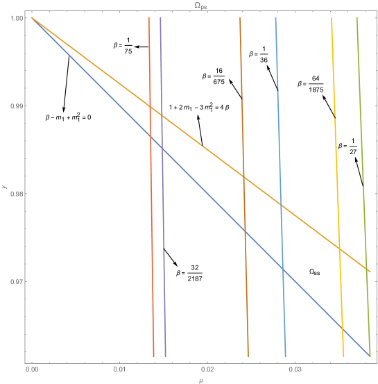
Figure 2: masses space $\Omega_{ps}$ and resonance

$$\Omega_{ps}=\{(\beta,m_{1})\in\Omega_{ss}:\beta\in(0,\frac{1}{27})\setminus\{\frac{1}{75},\frac{32}{2187},\frac{16}{675},\frac{1}{36},\frac{64}{1875}\}\},$$ (5.39)

please see Figure 2. Taking the resonance relations (5.35) into consideration, from now on, we confine ourselves to the masses in $\Omega_{ps}$.

6 KAM Stability

In this section, let us investigate the KAM stability (i.e., stability in the sense of measure) of Lagrange relative equilibrium. The main result is the following theorem.

Theorem 6.1

Possibly except the following cases corresponding to resonance

$$\begin{array}[]{c}\beta=\frac{1}{75};\beta=\frac{32}{2187};\beta=\frac{16}{675};\beta=\frac{1}{36};\beta=\frac{64}{1875},\end{array}$$

for every choice of masses of the planar three-body problem satisfying $\beta<\frac{1}{27}$, there are a great quantity of KAM invariant tori (or quasi-periodic solutions) in a small neighbourhood of Lagrange relative equilibrium. Furthermore, these tori form a set whose relative measure rapidly tends to 1 as the neighbourhood shrinks to zero; in particular, the relative measure exponentially tends to 1 for almost every choice of the masses.

As a corollary, we have the following result:

Theorem 6.2

Possibly except the following cases corresponding to resonance

$$\begin{array}[]{c}\beta=\frac{1}{75};\beta=\frac{32}{2187};\beta=\frac{16}{675};\beta=\frac{1}{36};\beta=\frac{64}{1875}\end{array}$$

for every choice of masses of the planar three-body problem satisfying $\beta<\frac{1}{27}$, Lagrange relative equilibrium is KAM stable.

Before proving Theorem 6.1, let us recall a classical result on real algebraic varieties.

Definition 6.1

([39]) An algebraic partial manifold $P$ in $\mathbb{R}^{n}$ is a point set, associated with a number $\nu$, with the following property. Take any $p\in P$. Then there exists a set of polynomials $f_{1},\cdots,f_{\nu}$ of rank $\nu$ at $p$ (i.e., the number of independent differential $df_{1}(p),\cdots,df_{\nu}(p)$ is $\nu$), and a neighborhood $\mathcal{N}$ of $p$, such that $P\bigcap\mathcal{N}$ is the set of zeros in $\mathcal{N}$ of these $f_{j}$. The number $n-\nu$ is the dimension of the partial manifold.

Theorem 6.3

([39]) Let $V\subset\mathbb{R}^{n}$ be a real algebraic variety, then $V$ can be split as a union of a finite number of partial algebraic manifolds:

$$V=P_{1}\bigcup P_{2}\bigcup\cdots\bigcup P_{s},$$

each $P_{j}$ being an algebraic partial manifold in $V$, and the $P_{j}$ being disjoint. Here, the dimension $n_{j}$ of $P_{j}$ are decrease. Furthermore, $s\leq 2^{n}-1$ and each $P_{j}$ has but a finite number of topological components.

Proof of Theorem 6.1:

First, let us investigate degeneracy and isoenergetical degeneracy of the the Hamiltonian (5.38).

A straight forward computation shows that

$$det\left(\begin{array}[]{ccc}\omega_{00}&\omega_{01}&\omega_{02}\\ \omega_{01}&\omega_{11}&\omega_{12}\\ \omega_{02}&\omega_{12}&\omega_{22}\\ \end{array}\right)=\frac{-27\beta}{128(16-675\beta)^{2}(1-36\beta)^{2}\gamma^{4}m_{1}^{2}m_{2}^{2}m_{3}^{2}}f_{deg}$$ (6.40)

and

$$det\left(\begin{array}[]{cccc}\omega_{00}&\omega_{01}&\omega_{02}&\omega_{0}\\ \omega_{01}&\omega_{11}&\omega_{12}&-\omega_{1}\\ \omega_{02}&\omega_{12}&\omega_{22}&\omega_{2}\\ \omega_{0}&-\omega_{1}&\omega_{2}&0\\ \end{array}\right)=\frac{-27\beta f_{isodeg}}{64(16-675\beta)^{2}(1-36\beta)^{2}(1-27\beta)^{2}m_{1}^{2}m_{2}^{2}m_{3}^{2}},$$ (6.41)

where

$$f_{deg}=\frac{2(1-36\beta)^{2}}{3}(52542675\beta^{3}+178185258\beta^{2}-9896841\beta-47632)\beta^{4}$$

$$-11(397050199920\beta^{5}-40790893923\beta^{4}+4055047758\beta^{3}-243771759\beta^{2}+6417616\beta$$

$$-59392)\beta^{3}m_{1}+(5465578392450\beta^{6}+19309935720393\beta^{5}-3995019640449\beta^{4}$$

$$+327340481715\beta^{3}-13039336341\beta^{2}+250520816\beta-1857536)\beta^{2}m_{1}^{2}+(2408448$$

$$-15298708984020\beta^{6}-29436067209393\beta^{5}+7048034089254\beta^{4}-562788423405\beta^{3}$$

$$+20645100208\beta^{2}-359200768\beta)\beta m_{1}^{3}+3[(1821859464150\beta^{6}+4980794507091\beta^{5}$$

$$-1182106602432\beta^{4}+94244985459\beta^{3}-3452615664\beta^{2}+59975680\beta-401408)$$

$$m_{1}^{4}(2\beta+m_{1}^{2}-2m_{1}+1)],$$

$$f_{isodeg}=(1-36\beta)^{2}(52542675\beta^{3}+178185258\beta^{2}-9896841\beta-47632)\beta^{4}$$

$$-6(1114633724580\beta^{5}-129174146793\beta^{4}+12399204438\beta^{3}-701681085\beta^{2}+17908688\beta$$

$$-163328)\beta^{3}m_{1}+3(2856548519100\beta^{6}+9467506918989\beta^{5}-1979796586608\beta^{4}$$

$$+162904807989\beta^{3}-6502400730\beta^{2}+125103520\beta-928768)\beta^{2}m_{1}^{2}-24(992795560920\beta^{6}$$

$$+1777266330759\beta^{5}-427262272146\beta^{4}+34351179507\beta^{3}-1270282468\beta^{2}+22280704\beta$$

$$-150528)\beta m_{1}^{3}+9(952182839700\beta^{6}+2412746489943\beta^{5}-573816097674\beta^{4}$$

$$+46035466371\beta^{3}-1699679520\beta^{2}+29762048\beta-200704)m_{1}^{4}(2\beta+m_{1}^{2}-2m_{1}+1).$$

Therefore, the Hamiltonian (5.38) is non-degenerate if and only if $f_{deg}\neq 0$, and the Hamiltonian (5.38) is isoenergetically non-degenerate if and only if $f_{isodeg}\neq 0$. Thus the set $V_{f_{deg}}$ of points $(\beta,m_{1})$ such that the Hamiltonian (5.38) is degenerate is a real algebraic variety. So is the set $V_{f_{isodeg}}$ of isoenergetically degenerate. By Theorem 6.3, it follows that each of $V_{f_{deg}}$ and $V_{f_{isodeg}}$ is an union of a finite number of zero-dimensional points and one-dimensional “curves”. To make the direct-viewing understanding of the real algebraic varieties $V_{f_{deg}}$ and $V_{f_{isodeg}}$, we give the plots of zero locus sets of $f_{deg}$ and $f_{isodeg}$, please see Figure 3.

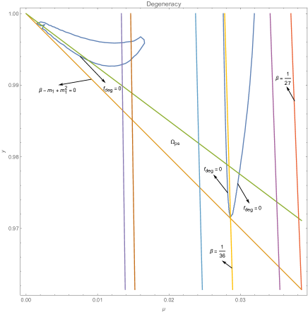
Figure 3: plots of $V_{f}$ and $V_{g}$

So the Hamiltonian (5.38) is non-degenerate and isoenergetically non-degenerate for almost every choices of $(\beta,m_{1})$. Furthermore, a straight forward computation shows that $f$ and $g$ can not be 0 at the same time in the space of masses $\Omega_{ps}$.

As a result, it follows from Theorem 4.1, Theorem 4.2 and Theorem 5.1 that Theorem 6.1 holds.

$~{}~{}~{}~{}~{}~{}~{}~{}~{}~{}~{}~{}~{}~{}~{}~{}~{}~{}~{}~{}~{}~{}~{}~{}~{}~{}~{}~{}~{}~{}~{}~{}~{}~{}~{}~{}~{}~{}~{}~{}~{}~{}~{}~{}~{}~{}~{}~{}~{}~{}~{}~{}~{}~{}~{}~{}~{}~{}~{}~{}~{}~{}~{}~{}~{}~{}~{}~{}~{}~{}~{}~{}~{}~{}~{}~{}~{}~{}~{}~{}~{}~{}~{}~{}~{}~{}~{}~{}~{}~{}~{}~{}~{}~{}~{}~{}~{}~{}~{}~{}~{}~{}~{}~{}~{}~{}~{}~{}~{}~{}~{}~{}~{}~{}~{}~{}~{}~{}~{}~{}~{}~{}~{}~{}~{}~{}~{}~{}~{}~{}~{}~{}~{}~{}~{}~{}~{}~{}~{}~{}~{}~{}~{}~{}~{}~{}~{}~{}~{}~{}~{}~{}~{}~{}~{}~{}~{}~{}~{}~{}~{}~{}~{}\Box$

7 Effective Stability

We now turn to effective stability.

First, it follows from Theorem 4.3 and Theorem 5.1 that

Theorem 7.1

For almost every choice of masses of the planar three-body problem satisfying $\beta\in(0,\frac{1}{27})$, there exists a small neighbourhood $\mathcal{N}$ of Lagrange relative equilibrium such that, for every orbit $(\varrho(t),\varphi(t))$ whose initial value is in $\mathcal{N}$, one has

$$\|\varrho(t)-\varrho(0)\|\leq c_{1}\epsilon^{3}~{}~{}~{}~{}~{}~{}~{}~{}~{}~{}~{}~{}~{}~{}for~{}~{}~{}|t|\leq c_{3}\exp(c_{2}\epsilon^{-b}),$$

provided $\epsilon$ is sufficiently small, here $c_{1},c_{2},c_{3}=const>0$ and the constant $b$ is any number in the interval $(0,\frac{1}{7})$. Therefore, Lagrange relative equilibrium is exponentially stable for almost every choice of masses of the planar three-body problem such that $\beta<\frac{1}{27}$.

On the one hand, the masses in Theorem 7.1 yielding exponential stability are abundant in measure. On the other hand, the masses in Theorem 7.1 may be quite exceptional in some sense. For example, according to Theorem 5.1, the masses which can not yield exponential stability are dense. Therefore, it is not allowed to have measuring error of masses for applying Theorem 7.1, however it is impossible for no measuring error of masses in practice.

So let us investigate directional quasi-convexity of the Birkhoff normal form $\mathcal{H}_{B4}(\varrho)$.

As a matter of convenience, first of all, let us give the following result.

Lemma 7.2

The Birkhoff normal form $\mathcal{H}_{B4}(\varrho)$ is

• convex at $\varrho=0$, if and only if

  $$det\left(\begin{array}[]{cc}\omega_{00}&\omega_{01}\\ \omega_{01}&\omega_{11}\\ \end{array}\right)>0,det\left(\begin{array}[]{ccc}\omega_{00}&\omega_{01}&\omega_{02}\\ \omega_{01}&\omega_{11}&\omega_{12}\\ \omega_{02}&\omega_{12}&\omega_{22}\\ \end{array}\right)<0;$$

• quasi-convex at $\varrho=0$, if and only if

  $$a_{0}a_{2}-a_{1}^{2}>0;$$

• directionally quasi-convex at $\varrho=0$, if and only if

  $$\left\{\begin{array}[]{lr}a_{0}\neq 0&\\ a_{2}=0&\\ a_{0}(a_{0}+2a_{1}\frac{\mu_{1}}{\mu_{2}})>0&\end{array}\right.$$

  or

  $$\left\{\begin{array}[]{lr}a_{0}\neq 0~{}and~{}a_{2}\neq 0&\\ a_{0}h(\frac{\mu_{1}}{\mu_{2}})>0&\\ -\frac{a_{1}}{a_{2}})\notin[0,\frac{\mu_{1}}{\mu_{2}}]&\end{array}\right.$$

  or

  $$\left\{\begin{array}[]{lr}a_{0}\neq 0~{}and~{}a_{2}\neq 0&\\ a_{0}h(\frac{\mu_{1}}{\mu_{2}})>0&\\ a_{0}h(-\frac{a_{1}}{a_{2}}))>0&\\ -\frac{a_{1}}{a_{2}}\in[0,\frac{\mu_{1}}{\mu_{2}}]&\end{array}\right.$$

where

$$\begin{array}[]{c}a_{0}=\omega_{00}\mu_{1}^{2}+2\omega_{01}\mu_{1}+\omega_{11},\\ a_{1}=-\omega_{00}\mu_{1}\mu_{2}+\omega_{02}\mu_{1}-\omega_{01}\mu_{2}+\omega_{12},\\ a_{2}=\omega_{00}\mu_{2}^{2}-2\omega_{02}\mu_{2}+\omega_{22},\\ h(x)=a_{0}+2a_{1}x+a_{2}x^{2}.\end{array}$$

Proof. Recall that

$$\mathcal{H}_{B4}(\varrho)=\omega_{0}\varrho_{0}-\omega_{1}\varrho_{1}+\omega_{2}\varrho_{2}+\frac{1}{2}[\omega_{00}\varrho_{0}^{2}+\omega_{11}\varrho_{1}^{2}+\omega_{22}\varrho_{2}^{2}$$ (7.42)

$$+2\omega_{01}\varrho_{0}\varrho_{1}+2\omega_{02}\varrho_{0}\varrho_{2}+2\omega_{12}\varrho_{1}\varrho_{2}].$$

By $\omega_{00}=-3$, it follows that $\mathcal{H}_{B4}(\varrho)$ is convex at $\varrho=0$ if and only if the quadratic form

$$\omega_{00}\varrho_{0}^{2}+\omega_{11}\varrho_{1}^{2}+\omega_{22}\varrho_{2}^{2}+2\omega_{01}\varrho_{0}\varrho_{1}+2\omega_{02}\varrho_{0}\varrho_{2}+2\omega_{12}\varrho_{1}\varrho_{2}$$

is negative definite, that is,

$$det\left(\begin{array}[]{cc}\omega_{00}&\omega_{01}\\ \omega_{01}&\omega_{11}\\ \end{array}\right)>0,det\left(\begin{array}[]{ccc}\omega_{00}&\omega_{01}&\omega_{02}\\ \omega_{01}&\omega_{11}&\omega_{12}\\ \omega_{02}&\omega_{12}&\omega_{22}\\ \end{array}\right)<0.$$

Thanks to

$$\omega_{0}\varrho_{0}-\omega_{1}\varrho_{1}+\omega_{2}\varrho_{2}=0,$$

or

$$\varrho_{0}=\lambda_{1}\varrho_{1}-\lambda_{2}\varrho_{2},$$

the quadratic form

$$\omega_{00}\varrho_{0}^{2}+\omega_{11}\varrho_{1}^{2}+\omega_{22}\varrho_{2}^{2}+2\omega_{01}\varrho_{0}\varrho_{1}+2\omega_{02}\varrho_{0}\varrho_{2}+2\omega_{12}\varrho_{1}\varrho_{2}$$

reduces to the quadratic form

$$a_{0}\varrho_{1}^{2}+a_{2}\varrho_{2}^{2}+2a_{1}\varrho_{1}\varrho_{2}.$$

Then it is evident to see that $\mathcal{H}_{B4}(\varrho)$ is quasi-convex at $\varrho=0$, if and only if

$$a_{0}a_{2}-a_{1}^{2}>0;$$

$\mathcal{H}_{B4}(\varrho)$ is directionally quasi-convex at $\varrho=0$, if and only if

$$\left\{\begin{array}[]{lr}\lambda_{1}\varrho_{1}\geq\lambda_{2}\varrho_{2}\geq 0&\\ a_{0}\varrho_{1}^{2}+a_{2}\varrho_{2}^{2}+2a_{1}\varrho_{1}\varrho_{2}=0&\end{array}\right.\Rightarrow\varrho_{1}=\varrho_{2}=0,$$

or $a_{0}\neq 0$ and the equation

$$h(x)=a_{0}+2a_{1}x+a_{2}x^{2}=0$$

has no roots in the interval $[0,\frac{\mu_{1}}{\mu_{2}}]$. As a result, it is easy to see that the theorem holds.

$~{}~{}~{}~{}~{}~{}~{}~{}~{}~{}~{}~{}~{}~{}~{}~{}~{}~{}~{}~{}~{}~{}~{}~{}~{}~{}~{}~{}~{}~{}~{}~{}~{}~{}~{}~{}~{}~{}~{}~{}~{}~{}~{}~{}~{}~{}~{}~{}~{}~{}~{}~{}~{}~{}~{}~{}~{}~{}~{}~{}~{}~{}~{}~{}~{}~{}~{}~{}~{}~{}~{}~{}~{}~{}~{}~{}~{}~{}~{}~{}~{}~{}~{}~{}~{}~{}~{}~{}~{}~{}~{}~{}~{}~{}~{}~{}~{}~{}~{}~{}~{}~{}~{}~{}~{}~{}~{}~{}~{}~{}~{}~{}~{}~{}~{}~{}~{}~{}~{}~{}~{}~{}~{}~{}~{}~{}~{}~{}~{}~{}~{}~{}~{}~{}~{}~{}~{}~{}~{}~{}~{}~{}~{}~{}~{}~{}~{}~{}~{}~{}~{}~{}~{}~{}~{}~{}~{}~{}~{}~{}~{}~{}~{}\Box$

Let $\Omega_{c},\Omega_{qc},\Omega_{dqc}$ be the subsets of the space $\Omega_{ps}$ of masses corresponding to convexity, quasi-convexity and directional quasi-convexity respectively. Then a straightforward computation shows that $\Omega_{c}$ is empty, that is, $\mathcal{H}_{B4}(\varrho)$ is not convex at $\varrho=0$ for any choice of masses of the three-body problem.

For quasi-convexity, a straightforward computation shows that

$$a_{0}a_{2}-a_{1}^{2}=-det\left(\begin{array}[]{cccc}\omega_{00}&\omega_{01}&\omega_{02}&\omega_{0}\\ \omega_{01}&\omega_{11}&\omega_{12}&-\omega_{1}\\ \omega_{02}&\omega_{12}&\omega_{22}&\omega_{2}\\ \omega_{0}&-\omega_{1}&\omega_{2}&0\\ \end{array}\right),$$

as a result,

$$a_{0}a_{2}-a_{1}^{2}>0\Leftrightarrow f_{isodeg}>0,$$

and $\Omega_{qc}$ is empty for $\frac{1}{75}<\beta<\frac{1}{36}$ and $\frac{64}{1875}<\beta<\frac{1}{27}$ but not for $0<\beta<\frac{1}{75}$ or $\frac{1}{36}<\beta<\frac{64}{1875}$. To make the direct-viewing understanding of the space $\Omega_{qc}$, please see Figure 3 and 4, note that the picture for $\Omega_{qc}$ is enlarged.

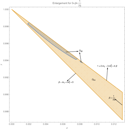
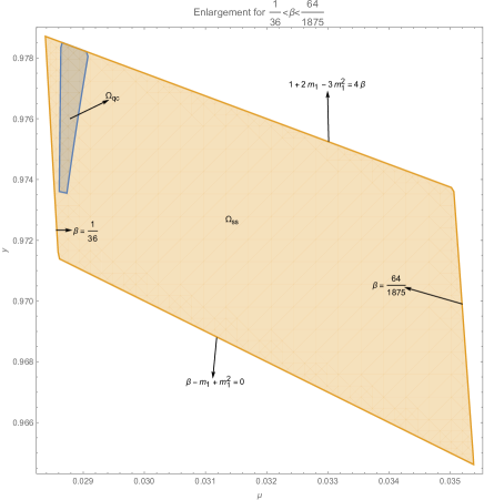
Figure 4: enlargement of $\Omega_{qc}$

For directional quasi-convexity, it follows from Lemma 7.2 that

$$\Omega_{dqc}=\Omega_{pdqc}\setminus\Omega_{ndqc},$$

here

$$\begin{array}[]{c}\Omega_{pdqc}=\{(\beta,m_{1})\in\Omega_{ps}:a_{0}h(\frac{\mu_{1}}{\mu_{2}})>0\},\\ \Omega_{ndqc}=\{(\beta,m_{1})\in\Omega_{pdqc}:a_{2}\neq 0,0<-\frac{a_{1}}{a_{2}}<\frac{\mu_{1}}{\mu_{2}},a_{0}h(-\frac{a_{1}}{a_{2}})\leq 0\}.\end{array}$$

Some tedious computation shows that $\Omega_{ndqc}$ is empty, and for $(\beta,m_{1})\in\Omega_{ps}$,

$$a_{0}h(\frac{\mu_{1}}{\mu_{2}})>0\Leftrightarrow f_{dqc}>0,$$

where

$$\begin{array}[]{lc}\begin{aligned} &f_{dqc}=[\frac{\left(236-62\gamma^{4}-479\gamma^{3}+1299\gamma^{2}-994\gamma\right)(\gamma+1)^{2}}{m_{1}m_{2}m_{3}}+729\left(76-401\gamma^{3}+81\gamma^{2}-18\gamma\right)]\\ &[\frac{3\beta\left(16-469476\beta^{3}+71469\beta^{2}-2199\beta\right)}{m_{1}m_{2}m_{3}}+\left(1509030\beta^{3}+2316519\beta^{2}-133983\beta+1936\right)].\end{aligned}\end{array}$$

As a result, the space $\Omega_{dqc}=\Omega_{pdqc}$ is a subset of $\Omega_{ps}$ satisfying $f_{dqc}>0$. It is easy to see that the space $\Omega_{dqc}$ is a large part of the space $\Omega_{ps}$ geometrically. To make the direct-viewing understanding of the space $\Omega_{dqc}$, please see Figure 5.

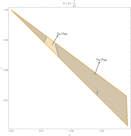
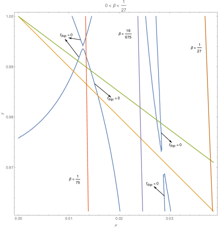
Figure 5: plots of $\Omega_{dqc}$

To sum up, we have

Theorem 7.3

The Birkhoff normal form $\mathcal{H}_{B4}(\varrho)$ is

• never convex at $\varrho=0$, i.e., $\Omega_{c}$ is empty;

• quasi-convex at $\varrho=0$, if and only if $(\beta,m_{1})\in\Omega_{qc}$, here

  $$\Omega_{qc}=\{(\beta,m_{1})\in\Omega_{ps}:f_{isodeg}>0,~{}\beta\in(0,\frac{1}{75})\bigcup(\frac{1}{36},\frac{64}{1875})\};$$

• directionally quasi-convex at $\varrho=0$, if and only if $(\beta,m_{1})\in\Omega_{dqc}$, here

  $$\Omega_{dqc}=\{(\beta,m_{1})\in\Omega_{ps}:f_{dqc}>0\}.$$

To study exponential stability, it suffices to consider directional quasi-convexity. Indeed, it follows from Theorem 4.4 that

Theorem 7.4

For every choice of masses of the planar three-body problem satisfying $(\beta,m_{1})\in\Omega_{dqc}$, there exists a small neighbourhood $\mathcal{N}$ of Lagrange relative equilibrium such that, for every orbit $(\varrho(t),\varphi(t))$ whose initial value is in $\mathcal{N}$, one has

$$\|\varrho(t)-\varrho(0)\|\leq c_{1}\epsilon^{a}~{}~{}~{}~{}~{}~{}~{}~{}~{}~{}~{}~{}~{}~{}for~{}~{}~{}|t|\leq c_{3}\exp(c_{2}\epsilon^{-b}),$$

provided $\epsilon$ is sufficiently small, here $c_{1},c_{2},c_{3}=const>0$ and the constants $a,b$ can be chosen as $a=\frac{1+\sigma}{n+\sigma},b=\frac{1}{n+\sigma}$ for any $\sigma\geq 0$. Therefore, Lagrange relative equilibrium is exponentially stable for every choice of masses in the space $\Omega_{dqc}$.

Remark 7.1

For a choice of masses in the space $\Omega_{ps}\setminus\Omega_{dqc}$, one should extend and apply a more general Theorem 4.4 to explore exponential stability. As a matter of fact, there is a more general Theorem 4.4 in [5] with a weaker condition than directional quasi-convexity, the condition is nearer to steepness, that is, the Birkhoff normal form $\mathcal{H}_{B6}(\varrho)$ is $3$-jet nondegenerate at $\varrho=0$. But the computation is too complicated to obtain the Birkhoff normal form $\mathcal{H}_{B6}(\varrho)$.

Let us give the following result that the Birkhoff normal form $\mathcal{H}_{B4}(\varrho)$ is steep, although there is no proof of a general Theorem 4.4 under the condition of steepness at present.

Theorem 7.5

Possibly except the following cases corresponding to resonance

$$\begin{array}[]{c}\beta=\frac{1}{75};\beta=\frac{32}{2187};\beta=\frac{16}{675};\beta=\frac{1}{36};\beta=\frac{64}{1875},\end{array}$$

for every choice of masses of the planar three-body problem satisfying $\beta<\frac{1}{27}$, $\mathcal{H}_{B4}(\varrho)$ is steep in some neighbourhood ${B_{r_{\beta}}}$ of the origin, where

$$r_{\beta}=\frac{\beta^{3/4}}{\sqrt{5+\frac{9}{(1-36\beta)^{2}(1-27\beta)}+\frac{10^{6}}{(27\beta-1)^{2}(36\beta-1)^{2}(675\beta-16)^{2}m_{1}^{2}m_{2}^{2}m_{3}^{2}}}}.$$

Proof. We divide our proof in two steps.

First, for every choice of positive masses of the planar three-body problem satisfying $(\beta,m_{1})\in\Omega_{ps}$, we prove that $\mathcal{H}_{B4}(\varrho)$ has no critical points in $\overline{B_{r_{\beta}}}$. (step 1)

Assume the point $\varrho=(\varrho_{0},\varrho_{1},\varrho_{2})^{\top}$ is a critical point of $\mathcal{H}_{B4}(\varrho)$, then

$$\frac{\partial\mathcal{H}_{B4}}{\partial\varrho}=0,$$

or

$$W\varrho=-\varpi^{\top},$$ (7.43)

here

$$W=\frac{\partial^{2}\mathcal{H}_{B4}}{\partial\varrho^{2}}=\left(\begin{array}[]{ccc}\omega_{00}&\omega_{01}&\omega_{02}\\ \omega_{01}&\omega_{11}&\omega_{12}\\ \omega_{02}&\omega_{12}&\omega_{22}\\ \end{array}\right),$$

and $\varpi=(\omega_{0},-\omega_{1},\omega_{2})$ is the frequency vector.

It follows that

$$\omega_{0}^{2}+\omega_{1}^{2}+\omega_{2}^{2}\leq(\omega_{00}^{2}+\omega_{11}^{2}+\omega_{22}^{2}+2\omega_{01}^{2}+2\omega_{02}^{2}+2\omega_{12}^{2})(\varrho_{0}^{2}+\varrho_{1}^{2}+\varrho_{2}^{2}).$$ (7.44)

The aim is to prove that (7.44) yields the following estimation

$$\begin{array}[]{c}\frac{\omega_{0}^{2}+\omega_{1}^{2}+\omega_{2}^{2}}{\omega_{00}^{2}+\omega_{11}^{2}+\omega_{22}^{2}+2\omega_{01}^{2}+2\omega_{02}^{2}+2\omega_{12}^{2}}>r_{\beta}.\end{array}$$ (7.45)

A straightforward computation shows that the three equations

$$\omega_{11}=0,~{}~{}~{}~{}~{}~{}~{}~{}\omega_{22}=0,~{}~{}~{}~{}~{}~{}~{}~{}\omega_{12}=0$$

have no solution for $0<\beta<\frac{1}{27}$ and $0.96<m_{1}<1$, thus

$$\omega_{11}^{2}+\omega_{22}^{2}+2\omega_{12}^{2}>0.$$

By virtue of

$$\omega_{11}^{2}+\omega_{22}^{2}+2\omega_{12}^{2}=\frac{9}{32(27\beta-1)^{2}(36\beta-1)^{2}(675\beta-16)^{2}m_{1}^{2}m_{2}^{2}m_{3}^{2}}$$

$$[\frac{\beta^{4}(1-36\beta)^{2}}{3}(52542675\beta^{4}-254067678\beta^{3}+24800847\beta^{2}-387536\beta+3456)$$

$$+6(1092450983580\beta^{5}-177644083959\beta^{4}+12794359374\beta^{3}-478172835\beta^{2}$$

$$+8933708\beta-65728)\beta^{4}m_{1}-\beta^{2}m_{1}^{2}(8796996017100\beta^{7}+1736483408451\beta^{6}$$

$$-260078284944\beta^{5}+7108908219\beta^{4}+541625274\beta^{3}-40867544\beta^{2}+981888\beta$$

$$-8192)+4(6037174483920\beta^{7}-2675577372453\beta^{6}+422084648466\beta^{5}$$

$$-35545883265\beta^{4}+1718731704\beta^{3}-47333488\beta^{2}+688128\beta-4096)\beta m_{1}^{3}$$

$$-(8796996017100\beta^{7}-4818222493029\beta^{6}+805786218810\beta^{5}-69657248025\beta^{4}$$

$$+3410662284\beta^{3}-94469792\beta^{2}+1376256\beta-8192)m_{1}^{4}\left(2\beta+m_{1}^{2}-2m_{1}+1\right)],$$

it is easy to see that

$$\omega_{11}^{2}+\omega_{22}^{2}+2\omega_{12}^{2}<\frac{10^{6}}{(27\beta-1)^{2}(36\beta-1)^{2}(675\beta-16)^{2}m_{1}^{2}m_{2}^{2}m_{3}^{2}}$$

for $0<\beta<\frac{1}{27}$ and $0.96<m_{1}<1$.

Thanks to

$$2\omega_{01}^{2}+2\omega_{02}^{2}=\frac{9\left(775656\beta^{3}-63135\beta^{2}+1701\beta-16\right)}{8(1-36\beta)^{2}(27\beta-1)}$$

and

$$-16<775656\beta^{3}-63135\beta^{2}+1701\beta-16<-\frac{16}{81}~{}~{}~{}~{}~{}~{}~{}~{}for~{}~{}~{}~{}0<\beta<\frac{1}{27},$$

we have the following estimation

$$9+\frac{2}{9(1-36\beta)^{2}(1-27\beta)}<\omega_{00}^{2}+\omega_{11}^{2}+\omega_{22}^{2}+2\omega_{01}^{2}+2\omega_{02}^{2}+2\omega_{12}^{2}$$

$$<9+\frac{18}{(1-36\beta)^{2}(1-27\beta)}+\frac{10^{6}}{(27\beta-1)^{2}(36\beta-1)^{2}(675\beta-16)^{2}m_{1}^{2}m_{2}^{2}m_{3}^{2}}.$$

Consequently,

$$\begin{array}[]{c}\frac{\omega_{0}^{2}+\omega_{1}^{2}+\omega_{2}^{2}}{\omega_{00}^{2}+\omega_{11}^{2}+\omega_{22}^{2}+2\omega_{01}^{2}+2\omega_{02}^{2}+2\omega_{12}^{2}}>\frac{\beta^{3/2}}{5+\frac{9}{(1-36\beta)^{2}(1-27\beta)}+\frac{10^{6}}{(27\beta-1)^{2}(36\beta-1)^{2}(675\beta-16)^{2}m_{1}^{2}m_{2}^{2}m_{3}^{2}}},\end{array}$$

and it follows that $\mathcal{H}_{B4}(\varrho)$ has no critical points in $\overline{B_{r_{\beta}}}$.

Our task now is to prove that a restriction $\mathcal{H}_{B4}|_{\mathcal{P}}$ of $\mathcal{H}_{B4}(\varrho)$ to any proper affine subspace $\mathcal{P}\subset\mathbb{R}^{3}$ admits only isolated critical points. (step 2)

Suppose that $\mathcal{H}_{B4}(\varrho)$ admits nonisolated critical points in some proper affine subspace $\mathcal{P}\subset\mathbb{R}^{3}$, then by virtue of (7.43) and $\varpi\neq 0$, it follows that $\mathcal{P}$ is a two-dimensional plane. Let $\mathcal{P}=Span(\xi_{1},\xi_{2})$, $\xi_{1},\xi_{2}$ are independent. Then we have the relations

$$Rank(W\xi_{1},W\xi_{2},-\varpi^{\top})=Rank(W\xi_{1},W\xi_{2})=1$$ (7.46)

So the matrix $W$ is noninvertible, and the frequency vector $\varpi^{\top}$ belongs to the image set of linear operator $W$, in other words,

$$\varpi^{\top}\in Span(\left(\begin{array}[]{c}\omega_{00}\\ \omega_{01}\\ \omega_{02}\\ \end{array}\right),\left(\begin{array}[]{c}\omega_{01}\\ \omega_{11}\\ \omega_{12}\\ \end{array}\right),\left(\begin{array}[]{c}\omega_{02}\\ \omega_{12}\\ \omega_{22}\\ \end{array}\right)).$$ (7.47)

A straight forward computation shows that for every choice of masses satisfying $(\beta,m_{1})\in\Omega_{ps}$, $(\omega_{02},\omega_{12},\omega_{22})$ and $(\omega_{01},\omega_{11},\omega_{12})$ are independent. Hence

$$det\left(\begin{array}[]{ccc}\omega_{00}&\omega_{01}&\omega_{02}\\ \omega_{01}&\omega_{11}&\omega_{12}\\ \omega_{02}&\omega_{12}&\omega_{22}\\ \end{array}\right)=0,~{}~{}~{}~{}~{}det\left(\begin{array}[]{ccc}1&\omega_{01}&\omega_{02}\\ -\lambda_{1}&\omega_{11}&\omega_{12}\\ \lambda_{2}&\omega_{12}&\omega_{22}\\ \end{array}\right)=0.$$

Some tedious computation shows that for $(\beta,m_{1})\in\Omega_{ps}$, the equations above cannot hold at the same time.

So $\mathcal{H}_{B4}(\varrho)$ is steep in some neighbourhood ${B_{r_{\beta}}}$ of the original point for any $(\beta,m_{1})\in\Omega_{ps}$. The proof of Theorem 7.5 is now complete.

$~{}~{}~{}~{}~{}~{}~{}~{}~{}~{}~{}~{}~{}~{}~{}~{}~{}~{}~{}~{}~{}~{}~{}~{}~{}~{}~{}~{}~{}~{}~{}~{}~{}~{}~{}~{}~{}~{}~{}~{}~{}~{}~{}~{}~{}~{}~{}~{}~{}~{}~{}~{}~{}~{}~{}~{}~{}~{}~{}~{}~{}~{}~{}~{}~{}~{}~{}~{}~{}~{}~{}~{}~{}~{}~{}~{}~{}~{}~{}~{}~{}~{}~{}~{}~{}~{}~{}~{}~{}~{}~{}~{}~{}~{}~{}~{}~{}~{}~{}~{}~{}~{}~{}~{}~{}~{}~{}~{}~{}~{}~{}~{}~{}~{}~{}~{}~{}~{}~{}~{}~{}~{}~{}~{}~{}~{}~{}~{}~{}~{}~{}~{}~{}~{}~{}~{}~{}~{}~{}~{}~{}~{}~{}~{}~{}~{}~{}~{}~{}~{}~{}~{}~{}~{}~{}~{}~{}~{}~{}~{}~{}~{}~{}\Box$

8 Conclusion

For the planar three-body problem, based on the moving coordinates introduced in [40], which allows us to obtain a reduced system of equations of motion suitable for describing the motion of particles near relative equilibria, we mainly discussed the nonlinear stability of Lagrange relative equilibrium.

First, we proved that a relative equilibrium is orbitally stable if and only if the origin of the reduced system is Lyapunov stable. Before discussing the nonlinear stability, we gave some well known information on linear stability, and it is clear that it is more convenient to get the information by using the method based on the moving coordinates.

Next, it is necessary to get the Birkhoff normal form of the Hamiltonian near Lagrange triangular point. Although the construction of the normal form is simple in concept, but it is difficult to obtain the normal form. Thus this paper requires some computer assistance. Certainly, intensive computation cannot be avoided in celestial mechanics.

By virtue of the celebrated KAM theorem, we proved that Lagrange relative equilibrium is KAM stable, except possibly six special resonant cases, if it is spectrally stable. Indeed, there are a great quantity of KAM invariant tori in a small neighbourhood of Lagrange relative equilibrium, provided that the mass parameter $\beta\in(0,\frac{1}{27}]$, except possibly six special resonant cases $\beta=\frac{1}{75},\frac{32}{2187},\frac{16}{675},\frac{1}{36},\frac{64}{1875},\frac{1}{27}$. Furthermore, these tori or quasi-periodic solutions form a set whose relative measure rapidly tends to 1.

We also investigated the effective (exponential) stability of Lagrange relative equilibrium by the celebrated Nekhoroshev’s theory. First, we proved that Lagrange relative equilibrium is exponentially stable for almost every choice of positive masses of the planar three-body problem, except a dense but zero measure set of masses, if it is spectrally stable. Then we proved that Lagrange relative equilibrium is exponential stable for any choice of positive masses in a large open subset of spectrally stable space of masses. This large open subset is described by directional quasi-convexity.

Finally, we proved that the Birkhoff normal form of the Hamiltonian near Lagrange triangular point is steep provided that the mass parameter $\beta\in(0,\frac{1}{27}]$, except possibly six special resonant cases. This may be useful for further research of Lagrange relative equilibrium.

We hope to further explore the nonlinear stability problem of general relative equilibria in future work. We also hope that this work may spark the interest of using the moving coordinates among researchers.

We conclude this paper with a simple application of the results of stability to the Sun-Jupiter system ($\mu_{SJ}\approx 9.538753\cdot 10^{-4}$) and Earth-Moon system ($\mu_{EM}\approx 0.0121506$).

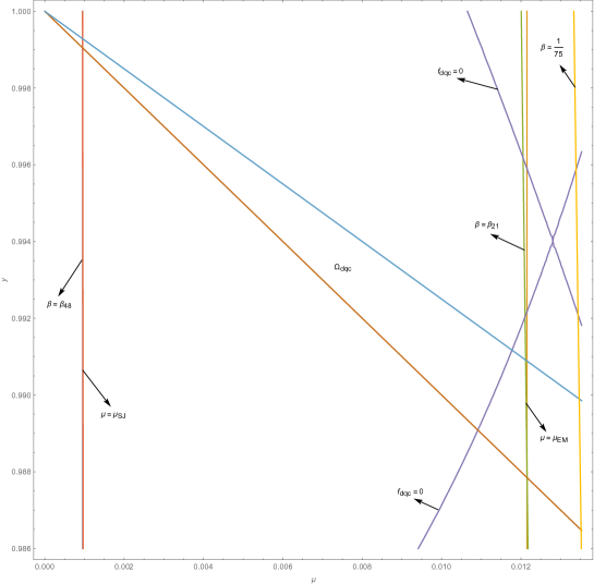
Figure 6: the Sun-Jupiter system and Earth-Moon system

First, each of Lagrange relative equilibria of the two systems is KAM stable, however we claim that the KAM stability on the Sun-Jupiter system is stronger than on the Earth-Moon system in some sense. In fact, we can claim that the speed of relative measure of KAM invariant tori tending to 1 for the Sun-Jupiter system is much faster than for the Earth-Moon system. Since the mass parameter $\beta$ first entering into the stability region, for the Sun-Jupiter system, is $\beta_{48}\approx 9.530527\cdot 10^{-4}$ corresponding to a resonance relation of order $48$; and, for the Earth-Moon system, is $\beta_{21}\approx 0.0120078$ corresponding to a resonance relation of order $21$.

For effective stability, we believe that each of Lagrange relative equilibria of the two systems is exponentially stable, although the Birkhoff normal form $\mathcal{H}_{B4}$ of degree $4$ is directionally quasi-convex for the Sun-Jupiter system but not for the Earth-Moon system. Indeed, we believe that one can prove the exponential stability of the Earth-Moon system by further calculating its Birkhoff normal form $\mathcal{H}_{B6}$ of degree $6$. On the other hand, we also believe that the stability worsens if the condition of directional quasi-convexity for $\mathcal{H}_{B4}$ is violated, that is, the exponential stability on the Sun-Jupiter system should be stronger than on the Earth-Moon system in some sense. As a matter of fact, in his celebrated 1977 article [29], Nekhoroshev also conjectured that different steepness properties should lead to numerically observable differences in the stability times, although it is not easy to prove this.

All in all, the work makes us believe that the stability of Lagrange relative equilibrium for the Earth-Moon system is weaker than for the Sun-Jupiter system. This should be partially one of the reasons that nobodies have been ever observed to gravitate around Lagrange triangular of the Earth-Moon system, but there are the well known Trojan asteroids around Lagrange triangular of the Sun-Jupiter system.

Appendix: on Lagrangian Dynamical Systems

For the sake of readability, we sketchily give the theory of Lagrangian dynamical systems used in deducing the general equations of motion. The exposition follows [2, 3], to which we refer the reader for proofs and details.

Definition 8.1

Let $\mathcal{M}$ be a differentiable manifold, $\mathrm{T}\mathcal{M}$ its tangent bundle, and $\mathcal{L}:\mathrm{T}\mathcal{M}\rightarrow\mathbb{R}$ a differentiable function. A map $\gamma:\mathbb{R}\rightarrow\mathcal{M}$ is called a motion in the Lagrangian system with configuration manifold $\mathcal{M}$ and Lagrangian function $\mathcal{L}$ if $\gamma$ is an extremal of the Lagrangian action functional

$$\mathcal{A}(\gamma)=\int^{t_{2}}_{t_{1}}{\mathcal{L}(\dot{\gamma}(t))dt}.$$

where $\dot{\gamma}$ is the velocity vector $\dot{\gamma}(t)\in\mathrm{T}_{\gamma(t)}\mathcal{M}$.

Theorem 8.1

The evolution of the local coordinates $q=(q_{1},\cdots,q_{n})$ of a point $\gamma(t)$ under motion in a Lagrangian system on a manifold satisfies the Euler-Lagrange equations

$$\frac{d}{dt}\frac{\partial\mathcal{L}}{\partial\dot{q}}=\frac{\partial\mathcal{L}}{\partial{q}},$$

where $\mathcal{L}(q,\dot{q})$ is the expression for the function $\mathcal{L}:\mathrm{T}\mathcal{M}\rightarrow\mathbb{R}$ in the coordinates $q$ and $\dot{q}$ on $\mathrm{T}\mathcal{M}$.

Theorem 8.1 yields a quick method for writing equations of motion in various coordinate systems, even in larger class of coordinate transformations which contain time. Indeed, to write the equations of motion in a new coordinate system, it is sufficient to express the Lagrangian function in the new coordinates. In fact, we have

Theorem 8.2

If the orbit $\gamma:q=\varphi(t)$ of Euler-Lagrange equations $\frac{d}{dt}\frac{\partial\mathcal{L}}{\partial\dot{q}}=\frac{\partial\mathcal{L}}{\partial{q}}$ is written as $\gamma:Q=\Phi(t)$ in the local coordinates $Q,t$ (where $Q=Q(q,t)$), then the function $\Phi(t)$ satisfies Euler-Lagrange equations $\frac{d}{dt}\frac{\partial\tilde{\mathcal{L}}}{\partial\dot{Q}}=\frac{\partial\tilde{\mathcal{L}}}{\partial{Q}}$, where $\tilde{\mathcal{L}}(Q,\dot{Q},t)=\mathcal{L}(q,\dot{q},t)$.

Remark 8.1

By the additional dependence of the Lagrangian function on time:

$$\mathcal{L}:\mathrm{T}\mathcal{M}\times\mathbb{R}\rightarrow\mathbb{R}~{}~{}~{}~{}~{}~{}\mathcal{L}=\mathcal{L}(q,\dot{q},t),$$

one can consider a Lagrangian nonautonomous system and the results above are also valid.

Definition 8.2

In mechanics, $\frac{\partial\mathcal{L}}{\partial\dot{q}}$ are called generalized momenta, $\frac{\partial\mathcal{L}}{\partial{q}}$ are called generalized forces.

Definition 8.3

Given a Lagrangian function $\mathcal{L}(q,\dot{q},t)$, a coordinate $q_{j}$ is called ignorable (or cyclic ) if it does not enter into the Lagrangian: $\frac{\partial\mathcal{L}}{\partial q_{j}}=0$.

Theorem 8.3

The generalized momentum corresponding to an ignorable coordinate is conserved: $p_{j}=\frac{\partial\mathcal{L}}{\partial\dot{q}_{j}}=const$.

The following content is Routh’s method for eliminating ignorable coordinates.
Suppose that the Lagrangian $\mathcal{L}(q,\dot{q},\dot{\xi})$ does not involve the coordinate $\xi$, i.e., $\xi$ is ignorable. Using the equality $\frac{\partial\mathcal{L}}{\partial\dot{\xi}}=c$ we represent the velocity $\dot{\xi}$ as a function of $q,\dot{q}$ and $c$. Following Routh we introduce the function

$$\mathcal{R}_{c}(q,\dot{q})=\mathcal{L}(q,\dot{q},\dot{\xi})-c\dot{\xi}|_{q,\dot{q},c}(=\mathcal{L}(q,\dot{q},\dot{\xi})-\frac{\partial\mathcal{L}}{\partial\dot{\xi}}\dot{\xi}|_{q,\dot{q},c}).$$

Theorem 8.4

A vector-function $(q(t),\xi(t))$ with the constant value of generalized momentum $\frac{\partial\mathcal{L}}{\partial\dot{\xi}}=c$ satisfies the Euler-Lagrange equations $\frac{d}{dt}\frac{\partial\mathcal{L}}{\partial\dot{q}}=\frac{\partial\mathcal{L}}{\partial{q}}$ if and only if $q(t)$ satisfies the Euler-Lagrange equations $\frac{d}{dt}\frac{\partial\mathcal{R}_{c}}{\partial\dot{q}}=\frac{\partial\mathcal{R}_{c}}{\partial{q}}.$

Example. Compare Newton’s equations (1.1)

$$\frac{d{m_{k}\dot{\mathbf{r}}_{k}}}{dt}-\frac{\partial\mathcal{U}}{\partial\mathbf{r}_{k}}=0,$$

with the Euler-Lagrange equations

$$\frac{d}{dt}\frac{\partial\mathcal{L}}{\partial\dot{q}}-\frac{\partial\mathcal{L}}{\partial{q}}=0$$

of Lagrangian system with configuration manifold $\mathcal{X}$ and Lagrangian function

$$\mathcal{L}=\mathcal{K}+\mathcal{U}.$$

Theorem 8.5

Motions of the mechanical system (1.1) coincide with extremals of the functional $\mathcal{A}(\mathbf{r})=\int^{t_{2}}_{t_{1}}{\mathcal{L}dt}.$

References

- [1] V.I. Arnold. Proof of a theorem of A. N. Kolmogorov on the invariance of quasi-periodic motions under small perturbations of the hamiltonian. Russian Mathematical Surveys, 18:9–36, 1963.
- [2] V.I. Arnold. Mathematical methods of classical mechanics. Translated by K. Vogtman and A. Weinstein, volume 60. Springer, New York, NY, 1978.
- [3] V.I. Arnold, V.V. Kozlov, and A.I. Neishtadt. Mathematical aspects of classical and celestial mechanics. Transl. from the Russian by E. Khukhro. 3rd revised. Berlin: Springer, 3rd revised ed. edition, 2006.
- [4] V.I. Arnold. Small denominators and problems of stability of motion in classical and celestial mechanics. Russian Mathematical Surveys, 18(6):85, 1963.
- [5] G. Benettin, F. Fassò, and M. Guzzo. Nekhoroshev–stability of L4 and L5 in the spatial restricted three-body problem. Regul. Chaotic Dyn, 3(3):56–72, 1998.
- [6] G.D. Birkhoff. Dynamical systems, volume 9. American Mathematical Society, Colloquium Publications, Vol. 9, New York, 1927.
- [7] A. Celletti and A. Giorgilli. On the stability of the Lagrangian points in the spatial restricted problem of three bodies. Celestial Mechanics and Dynamical Astronomy, 50(1):31–58, 1990.
- [8] L. Chierchia and G. Pinzari. The planetary n-body problem: symplectic foliation, reductions and invariant tori. Inventiones Mathematicae, 186(1):1–77, 2011.
- [9] A. Delshams and P. Gutiérrez. Estimates on invariant tori near an elliptic equilibrium point of a hamiltonian system. Journal of Differential Equations, 131(2):277–303, 1996.
- [10] A. Deprit and A. Deprit-Bartholome. Stability of the triangular Lagrangian points. The Astronomical Journal, volume 72 :173–179, 1967.
- [11] F. Fassò, M. Guzzo, and G. Benettin. Nekhoroshev-stability of elliptic equilibria of hamiltonian systems. Communications in Mathematical Physics, 197(2):347–360, 1998.
- [12] J. Féjoz. Démonstration du théorème d’arnold sur la stabilité du système planétaire (d’après herman). Ergodic Theory and Dynamical Systems, 24(5):1521–1582, 2004.
- [13] M. Gascheau. Examen d une classe d équations différentielles et applicationa un cas particulier du probleme des trois corps. Compt. Rend, 16(7):393–394, 1843.
- [14] A. Giorgilli. Rigorous results on the power expansions for the integrals of a hamiltonian system near an elliptic equilibrium point. In Annales de l’IHP Physique théorique, volume 48, pages 423–439, 1988.
- [15] A. Giorgilli. On the problem of stability for near to integrable hamiltonian systems. In Proceedings of the International Congress of Mathematicians Berlin, volume 3, pages 143–152, 1998.
- [16] A. Giorgilli, A. Delshams, E. Fontich, L. Galgani, and C. Sim . Effective stability for a hamiltonian system near an elliptic equilibrium point, with an application to the restricted three body problem. Journal of Differential Equations, 77(1):167–198, 1989.
- [17] A. Giorgilli and C. Skokos. On the stability of the trojan asteroids. Astronomy and Astrophysics, 317:254–261, 1997.
- [18] X. Hu, Y. Long, and S. Sun. Linear stability of elliptic Lagrangian solutions of the planar three-body problem via index theory. Archive for Rational Mechanics and Analysis, 213(3):993–1045, 2014.
- [19] X. Hu and S. Sun. Morse index and stability of elliptic Lagrangian solutions in the planar three-body problem. Advances in Mathematics, 223(1):98–119, 2010.
- [20] A.M. Leontovich. On the stability of the Lagrange periodic solutions of the restricted problem of three bodies. In Soviet Math. Dokl, volume 3, pages 425–428, 1962.
- [21] J.E. Littlewood. The Lagrange configuration in celestial mechanics. Proceedings of the London Mathematical Society, 3(4):525–543, 1959.
- [22] J.E. Littlewood. On the equilateral configuration in the restricted problem of three bodies. Proceedings of the London Mathematical Society, pages 640–640, 1959.
- [23] A.P. Markeev. Libration points in celestial mechanics and astrodynamics. Moscow Izdatel Nauka, 1978.
- [24] K.R. Meyer and D.S. Schmidt. Elliptic relative equilibria in the n-body problem. Journal of Differential Equations, 214(2):256–298, 2005.
- [25] K.R. Meyer and D.S. Schmidt. The stability of the Lagrange triangular point and a theorem of Arnold. Journal of Differential Equations, 62(2):222–236, 1986.
- [26] R. Moeckel. Linear stability analysis of some symmetrical classes of relative equilibria. In Hamiltonian Dynamical Systems, pages 291–317. Springer, 1995.
- [27] J. Moser. Stabilitätsverhalten kanonischer differentialgleichungssysteme. Nachr. Akad. Wiss. Gottingen. Math.-phys. Kl. Iia, 1955, 01 1955.
- [28] J. Moser. Lectures on Hamiltonian systems. Memoirs of the American Mathematical Society 81. American Mathematical Society, Providence, R.I. (1968).
- [29] N.N. Nekhoroshev. Exponential estimate of the stability time of near-integrable hamiltonian systems. Russ Math. Survey, 32:N6, 1977.
- [30] L. Niederman. Nonlinear stability around an elliptic equilibrium point in a hamiltonian system. Nonlinearity, 11(6):1465, 1998.
- [31] L. Niederman. Hamiltonian stability and subanalytic geometry. In Annales de l’institut Fourier, volume 56, pages 795–813, 2006.
- [32] F. Pacella. Central configurations of the n-body problem via equivariant morse theory. Archive for Rational Mechanics and Analysis, 97(1):59–74, 1987.
- [33] J. Pöschel. Integrability of hamiltonian systems on cantor sets. Communications on Pure and Applied Mathematics, 35(5):653–696, 1982.
- [34] J. Poschel. On nekhoroshev’s estimate at an elliptic equilibrium. International Mathematics Research Notices, 1999(4):203–215, 1999.
- [35] G.E. Roberts. Spectral instability of relative equilibria in the planar n-body problem. Nonlinearity, 12(4):757, 1999.
- [36] G.E. Roberts. Linear stability of the elliptic Lagrangian triangle solutions in the three-body problem. Journal of Differential Equations, 182(1):191–218, 2002.
- [37] E.J. Routh. On Laplace’s three particles, with a supplement on the stability of steady motion. Proceedings of the London Mathematical Society, 1(1):86–97, 1874.
- [38] A.G. Sokolskii. Proof of the stability of Lagrangian solutions for a critical mass ratio. Soviet Astronomy Letters, 4:79–81, 1978.
- [39] H. Whitney. Elementary structure of real algebraic varieties. Annals of Mathematics, pages 545–556, 1957.
- [40] X. Yu. On the problem of infinite spin in total collisions of the planar N-body problem. arXiv:1911.11006 [math.DS], 2019.