Continuous-time fully distributed generalized Nash equilibrium seeking for multi-integrator agents

Abstract

We consider strongly monotone games with convex separable coupling constraints, played by dynamical agents, in a partial-decision information scenario. We start by designing continuous-time fully distributed feedback controllers, based on consensus and primal-dual gradient dynamics, to seek a generalized Nash equilibrium in networks of single-integrator agents. Our first solution adopts a fixed gain, whose choice requires the knowledge of some global parameters of the game. To relax this requirement, we conceive a controller that can be tuned in a completely decentralized fashion, thanks to the use of uncoordinated integral adaptive weights. We further introduce algorithms specifically devised for generalized aggregative games. Finally, we adapt all our control schemes to deal with heterogeneous multi-integrator agents and, in turn, with nonlinear feedback-linearizable dynamical systems. For all the proposed dynamics, we show convergence to a variational equilibrium, by leveraging monotonicity properties and stability theory for projected dynamical systems.

, ,

1 Introduction

Generalized games arise in several engineering applications, including demand-side management in the smart grid (Saad et al., 2012), charging scheduling of electric vehicles (Grammatico, 2017) and communication networks (Facchinei and Pang, 2009). These scenarios involve multiple autonomous decision makers, or agents; each agent aims at minimizing its individual cost function – which depends on its own action as well as on the actions of other agents – subject to shared constraints. Specifically, in many distributed control problems, the action of an agent consists of the output of a dynamical system. For instance, in coverage maximization (Dürr et al., 2011) and connectivity problems (Stankovic et al., 2012), the agents are vehicles with some inherent dynamics, designed to optimize inter-dependent objectives related to their positions; in electricity markets, the actions are represented by the power produced by some generators (De Persis and Monshizadeh, 2019); in optical networks, the costs are a function of the output powers of some dynamical channels (Romano and Pavel, 2020).

In this context, the goal is to drive the physical processes to a desirable steady state, usually identified with a GNE, using only the local information available to each agent. One possibility is to exploit time-scale separation between the computation of a GNE and setpoint tracking; yet, this solution is typically economically inefficient and not robust (Zhang et al., 2015). Alternatively, part of the recent literature focuses on the design of distributed feedback controllers, to automatically steer a dynamical network to some (not known a priori) convenient operating point, while also ensuring closed-loop stability (De Persis and Monshizadeh, 2019; Dall’Anese et al., 2015). This paper fits in the latter framework.

In particular, we investigate GNE seeking for multi-integrator agents, motivated by robotics and mobile sensors applications (Frihauf et al., 2012; Stankovic et al., 2012), where multi-integrator dynamics are commonly used to model elementary vehicles. The study of this class of systems allows us to address GNE problems for a variety of dynamical agents, linear or nonlinear, via feedback linearization (e.g., Euler–Lagrangian systems as in Deng and Liang (2019)).

Literature review: A variety of algorithms has been proposed to seek a GNE in a distributed way (Yi and Pavel, 2019; Yu et al., 2017; Börgens and Kanzow, 2018) with a focus on aggregative games (Belgioioso and Grammatico, 2017; Paccagnan et al., 2016; De Persis and Grammatico, 2020). These works refer to (aggregative) games played in a full-decision information setting, where each agent can access the action of all the competitors (aggregate value), for example in presence of a central coordinator that broadcasts the data to the network. Nevertheless, this is impractical in many applications, where the agents only rely on local information.

Instead, in this paper, we consider the so-called partial-decision information scenario, where each agent holds an analytic expression for its cost but is unable to evaluate the actual value, since it cannot access the strategies of all the competitors. To remedy the lack of knowledge, the agents agree on sharing some information with some trusted neighbors over a communication graph. Based on the data exchanged, each agent can estimate and asymptotically reconstruct the actions of all the other agents. This setup has been investigated for games without coupling constraints, resorting to gradient and consensus dynamics, both in discrete-time (Tatarenko et al., 2018; Koshal et al., 2016), and continuous-time (Gadjov and Pavel, 2019; Ye and Hu, 2017). Fewer works deal with generalized games (Pavel, 2020; Deng and Nian, 2019; Parise et al., 2020). Moreover, all the results mentioned above consider static or single-integrator agents only. Distributively driving a network of more complex physical systems to a Nash equilibrium (NE) is still a relatively unexplored problem. With regard to aggregative games, a proportional integral feedback algorithm was developed in De Persis and Monshizadeh (2019) to seek a NE in networks of passive second-order systems; in Deng and Liang (2019) and Zhang et al. (2019), continuous-time gradient-based controllers were introduced for some classes of nonlinear dynamic. Stankovic et al. (2012) addressed generally coupled cost games played by linear agents, via an extremum seeking approach; NE problems in systems of multi-integrator agents were studied by Romano and Pavel (2020). Yet, none of these works considers generalized games. Despite the scarcity of results, the presence of shared constraints is a significant extension, which arises naturally when the agents compete for common resources (Facchinei and Kanzow, 2010, §2). However, dealing with coupling constraints in a distributed fashion is extremely challenging. All the results available resort to primal-dual reformulations (Pavel, 2020; Deng and Nian, 2019), where the main technical complications are the loss of monotonicity properties of the original problem and the non-uniqueness of dual solutions.

Contributions: Motivated by the above, we develop fully distributed continuous-time controllers to seek a GNE in networks of multi-integrator agents. We focus on games with separable coupling constraints, played under partial-decision information. Our novel contributions are summarized as follows:

• Nonlinear coupling constraints: We introduce primal-dual projected-gradient controllers to drive single-integrator agents to a GNE, with convergence guarantees under strong monotonicity and Lipschitz continuity of the game mapping. In contrast with the existing fully distributed methods, we allow for arbitrary convex separable (not necessarily affine) coupling constraints. Besides, our schemes are the only continuous-time fully distributed algorithms for generalized games (except for that in Deng and Nian (2019), for aggregative games and specific equality constraints only) (§3-4);

• Adaptive GNE seeking: We conceive the first GNE seeking algorithm that can be tuned in a fully decentralized way and without requiring any global information. Specifically, we extend the result in De Persis and Grammatico (2019) to generalized games and prove that convergence to an equilibrium can be ensured by adopting integral weights in place of a fixed, global, high-enough gain, whose choice would require the knowledge of the algebraic connectivity of the communication graph and of the Lipschitz and strong monotonicity constants of the game mapping (§3-4);

• Generalized aggregative games: We propose controllers for aggregative games with affine aggregation function, where the agents keep and exchange an estimate of the aggregation value only, thus reducing communication and computation cost. Differently from the existing results, e.g., Deng and Nian (2019), we can handle generic coupling constraints, thanks to a new variant of continuous-time dynamic tracking. Furthermore, we develop an adaptive algorithm that requires no a priori information and virtually no tuning (§5);

• Heterogeneous multi-integrator agents: We show how all our controllers can be adapted to solve GNE problems where each agent is described by mixed-order integrator dynamics, a class never considered before. Importantly, this allows us to address games played by arbitrary nonlinear agents with maximal relative degree, via feedback linearization. To the best of our knowledge, we are the first to study generalized games with higher-order dynamical agents (§6).

To improve readability, the proofs are in the appendix. Some preliminary results have been presented in Bianchi and Grammatico (2020); the novel contributions of this paper are: we consider adaptive controllers that can be tuned without need for any global information; we address a wider class of generalized games with nonlinear coupling constraints; we present algorithms for aggregative games, scalable with respect to the number of agents; we address the case of mixed-order multi-integrators (instead of double-integrators); we provide a more extensive numerical analysis, including applications to networks of heterogeneous nonlinear systems.

Basic notation: See Bianchi and Grammatico (2020).

Operator-theoretic definitions: An operator $\mathcal{F}:\mathbb{R}^{n}\rightarrow\mathbb{R}^{n}$ is monotone ($\mu$-strongly monotone) if, for all $x,y\in\mathbb{R}^{n}$, $(\mathcal{F}(x)-\mathcal{F}(y))^{\top}(x-y)\geq 0$ $(\geq\mu\|x-y\|^{2})$. For a closed convex set $S\subseteq\mathbb{R}^{n}$, $\mathrm{proj}_{S}:\mathbb{R}^{n}\rightarrow S$ is the Euclidean projection onto $S$; $\mathrm{N}_{S}:S\rightrightarrows\mathbb{R}^{n}:x\mapsto\{v\in\mathbb{R}^{n}\mid\sup_{z\in S}\,v^{\top}(z-x)\leq 0\}$ is the normal cone operator of $S$; $\mathrm{T}_{S}:S\rightrightarrows\mathbb{R}^{n}:x\mapsto\operatorname{cl}({\bigcup_{\delta>0}\frac{1}{\delta}(S-x)})$ is the tangent cone operator of $S$, where $\operatorname{cl}(\cdot)$ denotes the set closure. The projection on the tangent cone of $S$ at $x$ is $\Pi_{S}(x,v):=\mathrm{proj}_{\mathrm{T}_{S}(x)}(v)=\lim_{\delta\rightarrow 0^{+}}\textstyle\frac{\mathrm{proj}_{S}(x+\delta v)-x}{\delta}$. By Moreau’s Decomposition Theorem (Bauschke and Combettes, 2017, Th. 6.30), $v=\mathrm{proj}_{\mathrm{T}_{S}(x)}(v)+\mathrm{proj}_{\mathrm{N}_{S}(x)}(v)$ and $\mathrm{proj}_{\mathrm{T}_{S}(x)}(v)^{\top}\mathrm{proj}_{\mathrm{N}_{S}(x)}(v)=0$, for any $v\in\mathbb{R}^{n}$.

Projected dynamical systems (Cherukuri et al., 2016): Given an operator $\mathcal{F}:\mathbb{R}^{n}\rightarrow\mathbb{R}^{n}$ and a closed convex set $S\subseteq\mathbb{R}^{n}$, we consider the projected dynamical system

$$\dot{x}=\Pi_{S}(x,\mathcal{F}(x)),\qquad x(0)=x_{0}\in S.$$ (1)

In (1), the projection operator is possibly discontinuous on the boundary of $S$. If $\mathcal{F}$ is Lipschitz on $S$, the system (1) admits a unique global Carathéodory solution, i.e., there exists a unique absolutely continuous function $x:\mathbb{R}_{\geq 0}\rightarrow\mathbb{R}^{n}$ such that $x(0)=x_{0}$, $\dot{x}(t)=\Pi_{S}(x,g(x))$ for almost all $t$. Moreover, $x(t)\in S$ for all $t\geq 0$, as on the boundary of $S$ the projection operator restricts the flow of $\mathcal{F}$ such that the solution of (1) remains in $S$ (while $\Pi_{S}(x,\mathcal{F}(x))=\mathcal{F}(x)$ if $x\in\rm{int}(S)$).

Lemma 1.

Let $S\subseteq\mathbb{R}^{q}$ be a nonempty closed convex set. For any $y,y^{\prime}\in S$ and any $\xi\in\mathbb{R}^{q}$, it holds that $(y-y^{\prime})^{\top}\Pi_{S}\left(y,\xi\right)\leq(y-y^{\prime})^{\top}\xi$. In particular, if $\ \Pi_{S}(y,\xi)=0$, then $(y-y^{\prime})^{\top}\xi\geq 0$ (i.e., $\xi\in\mathrm{N}_{S}(y)$). $\square$

Proof. By Moreau’s theorem, $\left(\xi-\Pi_{S}(y,\xi)\right)\in\mathrm{N}_{S}(y)$; thus $\forall y,y^{\prime}\in S$, $(y^{\prime}-y)^{\top}(\xi-\Pi_{S}(y,\xi))\leq 0$. $\blacksquare$

2 Mathematical Background

We consider a group of agents $\mathcal{I}:=\{1,\ldots,N\}$, where each agent $i\in\mathcal{I}$ shall choose its decision variable (i.e., strategy) $x_{i}$ from its local decision set $\textstyle\Omega_{i}\subseteq\mathbb{R}^{n_{i}}$. Let $x:=\mathrm{col}((x_{i})_{i\in\mathcal{I}})\in\Omega$ denote the stacked vector of all the agents’ decisions, $\textstyle\Omega:=\times_{i\in\mathcal{I}}\Omega_{i}\subseteq\mathbb{R}^{n}$ the overall action space and $\textstyle n:=\sum_{i=1}^{N}n_{i}$. The goal of each agent $i\in\mathcal{I}$ is to minimize its objective function $J_{i}(x_{i},x_{-i})$, which depends both on the local strategy $x_{i}$ and on the decision variables of the other agents $x_{-i}:=\mathrm{col}((x_{j})_{j\in\mathcal{I}\backslash\{i\}})$. Furthermore, we address generalized games, where the coupling among the agents arises also via their feasible decision sets. In particular, we consider separable coupling constraints, so that the overall feasible set is $\mathcal{X}:=\textstyle\Omega\cap\left\{x\in\mathbb{R}^{n}\mid g(x)\leq\boldsymbol{0}_{m}\right\},$ where $g:\mathbb{R}^{n}\rightarrow\mathbb{R}^{m}$, $g(x):=\textstyle\sum_{i\in\mathcal{I}}g_{i}(x_{i})$, and $g_{i}:\mathbb{R}^{n_{i}}\rightarrow\mathbb{R}^{m}$ is a private function of agent $i$. The game is then represented by $N$ inter-dependent optimization problems:

$$\forall i\in\mathcal{I}:\;\underset{y_{i}\in\mathbb{R}^{n_{i}}}{\mathop{\rm argmin}}\;J_{i}(y_{i},x_{-i})\,\text{s.t. }\;(y_{i},x_{-i})\in\mathcal{X}.$$ (2)

The technical problem we consider in this paper is the computation of a GNE, a joint action from which no agent has interest to unilaterally deviate.

Definition 1.

A collective strategy $x^{*}=\operatorname{col}(\left(x_{i}^{*}\right)_{i\in\mathcal{I}})$ is a generalized Nash equilibrium if, for all $i\in\mathcal{I}$,

$${x_{i}^{*}\in\underset{y_{i}}{\mathop{\rm argmin}}\,J_{i}\left(y_{i},x_{-i}^{*}\right)\textup{ s.t. }(y_{i},x^{*}_{-i})\in\mathcal{X}.}$$

Next, we formulate standard convexity and regularity assumptions for the constraints and cost functions (Kulkarni and Shanbhag, 2012, Asm. 1; Pavel, 2020, Asm. 1).

Assumption 1.

For each $i\in\mathcal{I}$, the set $\Omega_{i}$ is closed and convex; $g_{i}$ is componentwise convex and twice continuously differentiable; $\mathcal{X}$ satisfies Slater’s constraint qualification; $J_{i}$ is continuously differentiable and the function $J_{i}\left(\cdot,x_{-i}\right)$ is convex for every $x_{-i}$. $\square$

Under Assumption 1, $x^{*}$ is a GNE of the game in (2) if and only if there exist dual variables $\lambda_{i}^{*}\in\mathbb{R}^{m}$ such that the following Karush–Kuhn–Tucker (KKT) KKT conditions are satisfied, for all $i\in\mathcal{I}$ (Facchinei and Kanzow, 2010, Th. 4.6):

Specifically, we focus on the subclass of variational GNE s (v-GNEs) (Facchinei and Kanzow, 2010, Def. 3.11), namely GNEs with equal dual variables, i.e. $\lambda_{i}^{*}=\lambda^{*}\in\mathbb{R}^{m}$ for all $i\in\mathcal{I}$, for which the KKT conditions read as

$${\boldsymbol{0}_{n}} \in F\left(x^{*}\right)+\textstyle\frac{\partial}{\partial x}g(x^{*})^{\top}\lambda^{*}+\mathrm{N}_{\Omega}(x^{*})$$ (3a)

$${\boldsymbol{0}_{m}} \in-g(x^{*})+\mathrm{N}_{\mathbb{R}_{\geq 0}}^{m}\left(\lambda^{*}\right).$$ (3b)

where $F$ is the pseudo-gradient mapping of the game:

$$F(x):=\operatorname{col}\left((\nabla_{\!\!x_{i}}J_{i}(x_{i},x_{-i})\right)_{i\in\mathcal{I}}).$$ (4)

Variational equilibria enjoys important structural properties, such as economic fairness (Facchinei and Kanzow, 2010). For example, in electricity markets, the dual variables correspond to unitary prices charged for the use of the infrastructure by an administrator that aim at maximizing its revenue while ensuring certain operating conditions, and it is reasonable to assume that the administrator cannot charge discriminatory prices to different energy producers (Kulkarni and Shanbhag, 2012). A sufficient condition for the existence and uniqueness of a v-GNE is the strong monotonicity of the pseudo-gradient (Yi and Pavel, 2019, Th. 1, Rem. 1), which was always postulated in continuous-time NE seeking under partial-decision information (Gadjov and Pavel, 2019, Asm. 2; Deng and Nian, 2019, Asm. 3). It implies strong convexity of the functions $J_{i}(\cdot,x_{-i})$ for any $x_{-i}$ (Tatarenko et al., 2018, Rem. 1), but not necessarily convexity of $J_{i}$ in the full argument.

Assumption 2.

The game mapping $F$ in (4) is:

• $\mu$-strongly monotone, for some $\mu>0$;

• $\theta_{0}$-Lipschitz continuous, for some $\theta_{0}>0$. $\square$

3 Fully distributed equilibrium seeking

In this section, we consider the game in (2), where each agent is associated with the following dynamical system:

$$\textstyle\forall i\in\mathcal{I}:\quad\dot{x}_{i}=u_{i},\ x_{i}(0)\in\Omega_{i}.$$ (5)

Our aim is to design the inputs $u_{i}\in\mathbb{R}^{n_{i}}$ to seek a v-GNE in a fully distributed way. Specifically, each agent $i\in\mathcal{I}$ only knows its own feasible set $\Omega_{i}$, the portion $g_{i}$ of the coupling constraints, and its own cost function $J_{i}$. Moreover, the agents cannot access the strategies of all the competitors $x_{-i}$. Instead, each agent only relies on the information exchanged locally with some neighbors over a communication network $\mathcal{G}(\mathcal{I},\mathcal{E})$. The unordered pair $(i,j)$ belongs to the set of edges $\mathcal{E}$ if and only if agent $i$ and $j$ can exchange information. We denote by $W\in\mathbb{R}^{N\times N}$ the symmetric adjacency matrix of $\mathcal{G}$, with $[W]_{i,j}>0$ if $(i,j)\in\mathcal{E}$, $[W]_{i,j}=0$ otherwise; $L$ the symmetric Laplacian matrix of $\mathcal{G}$; $\mathcal{N}_{i}:=\{j\mid(i,j)\in\mathcal{E}\}$ the set of neighbors of agent $i$. For ease of notation, we assume that the graph is unweighted, i.e., $[W]_{i,j}=1$ if $(i,j)\in\mathcal{E}$, but our results still hold for the weighted case.

Assumption 3.

The communication graph $\mathcal{G}(\mathcal{I},\mathcal{E})$ is undirected and connected. $\square$

Our first algorithm is inspired by the discrete-time primal-dual gradient iteration in (Pavel, 2020, Alg. 1). To cope with the lack of knowledge, the general assumption for the partial-decision information scenario is that each agent keeps an estimate of all other agents’ actions (Pavel, 2020; Tatarenko et al., 2018). Let $\boldsymbol{x}^{i}:=\operatorname{col}((\boldsymbol{x}^{i}_{j})_{j\in\mathcal{I}})\in\mathbb{R}^{n}$, where $\boldsymbol{x}^{i}_{i}:=x_{i}$ and $\boldsymbol{x}^{i}_{j}$ is agent $i$’s estimate of agent $j$’s action, for all $j\neq i$; $\boldsymbol{x}^{j}_{-i}:=\mathrm{col}((\boldsymbol{x}_{j,\ell})_{\ell\in\mathcal{I}\backslash\{i\}})$. Each agent also keeps an estimate $\lambda_{i}\in\mathbb{R}_{\geq 0}^{m}$ of the dual variable and an auxiliary variable $z_{i}\in\mathbb{R}^{m}$ to allow for distributed consensus of the dual estimates. Our proposed dynamics are summarized in Algorithm 3, where $c>0$ is a global fixed parameter (and $\theta$ is a constant defined in Lemma 3).

Algorithm 1 Constant gain

Initialization: set $c>\underline{c}:=\frac{(\theta_{0}+\theta)^{2}+4\mu\theta}{4\mu\uplambda_{2}(L)}$; $\forall i\in\mathcal{I}$, set $\boldsymbol{x}^{i}_{-i}(0)\in\mathbb{R}^{n-n_{i}}$, $z_{i}(0)=\boldsymbol{0}_{m}$, $\lambda_{i}(0)\in\mathbb{R}^{m}_{\geq 0}$;

Dynamics: $\forall i\in\mathcal{I},$

$$\begin{aligned} \dot{x}_{i}&=u_{i}=\Pi_{\Omega_{i}}(\begin{multlined}x_{i},-\nabla_{\!\!x_{i}}J_{i}(x_{i},\boldsymbol{x}^{i}_{-i})-\textstyle\frac{\partial}{\partial x_{i}}g_{i}(x_{i})^{\top}\lambda_{i}\\ -c{\textstyle\sum_{j\in\mathcal{N}_{i}}}(x_{i}-\boldsymbol{x}_{i}^{j}))\end{multlined}x_{i},-\nabla_{\!\!x_{i}}J_{i}(x_{i},\boldsymbol{x}^{i}_{-i})-\textstyle\frac{\partial}{\partial x_{i}}g_{i}(x_{i})^{\top}\lambda_{i}\\ -c{\textstyle\sum_{j\in\mathcal{N}_{i}}}(x_{i}-\boldsymbol{x}_{i}^{j}))\\ \dot{\boldsymbol{x}}^{i}_{-i}&=-c\textstyle\sum_{j\in\mathcal{N}_{i}}(\boldsymbol{x}_{-i}^{i}-\boldsymbol{x}_{-i}^{j})\\ {\dot{z}}_{i}&=\textstyle\sum_{j\in\mathcal{N}_{i}}(\lambda_{i}-\lambda_{j})\\ \dot{\lambda}_{i}&=\Pi_{\mathbb{R}_{\geq 0}^{m}}(\lambda_{i},g_{i}(x_{i})-z_{i}-\textstyle\sum_{j\in\mathcal{N}_{i}}(\lambda_{i}-\lambda_{j}))\end{aligned}$$

We note that the agents exchange $\{\boldsymbol{x}^{i},\lambda_{i}\}$ with their neighbors only, therefore the controller can be implemented distributedly. Importantly, each agent $i$ evaluates the partial gradient of its cost $\nabla_{\!\!x_{i}}J_{i}$ on its local estimate $\boldsymbol{x}^{i}$, not on the actual joint strategy $x$. In steady state, the agents should agree on their estimates, i.e., $\boldsymbol{x}^{i}=\boldsymbol{x}^{j},\ \lambda_{i}=\lambda_{j}$, for all $i,j\in\mathcal{I}$. This motivates the presence of consensual terms for both primal and dual variables. For any integer $q$, we denote $\boldsymbol{E}_{q}:=\{\boldsymbol{y}\in\mathbb{R}^{Nq}:\boldsymbol{y}={\boldsymbol{1}}_{N}\otimes y,y\in\mathbb{R}^{q}\}$ the consensus subspace of dimension $q$, and $\boldsymbol{E}_{q}^{\perp}:=\{\boldsymbol{y}\in\mathbb{R}^{Nq}:\left(\mathbf{1}_{N}^{\top}\otimes I_{q}\right)\boldsymbol{y}=\mathbf{0}_{q}\}$ its orthogonal complement; Specifically, $\boldsymbol{E}_{n}$ and $\boldsymbol{E}_{m}$ are the action and multiplier consensus subspaces, respectively. Moreover, $P_{q}:=\textstyle\frac{1}{N}{\boldsymbol{1}}_{N}{\boldsymbol{1}}_{N}^{\top}\otimes I_{q}$ is the projection matrix onto $\boldsymbol{E}_{q}$, i.e., $P_{q}\boldsymbol{y}=\mathrm{proj}_{\boldsymbol{E}_{q}}(\boldsymbol{y})$, and $P^{\perp}_{q}:=I_{Nq}-P_{q}$ the projection matrix onto the disagreement subspace $\boldsymbol{E}^{\perp}_{q}$.

Algorithm 2 Adaptive gains

Initialization: $\forall i\in\mathcal{I}$, set $\gamma_{i}>0$, $\boldsymbol{x}^{i}_{-i}(0)\in\mathbb{R}^{n-n_{i}}$, $k_{i}(0)\in\mathbb{R}$, $z_{i}(0)=\boldsymbol{0}_{m}$, $\lambda_{i}(0)\in\mathbb{R}^{m}$;

Dynamics: $\forall i\in\mathcal{I}$,

$$\begin{aligned} \dot{x}_{i}&=u_{i}=\Pi_{\Omega_{i}}\begin{multlined}(x_{i},-\nabla_{\!\!x_{i}}J_{i}(x_{i},\boldsymbol{x}_{-i}^{i})-\textstyle\frac{\partial}{\partial x_{i}}g_{i}(x_{i})^{\top}\lambda_{i}\\ -{\textstyle\sum_{j\in\mathcal{N}_{i}}}(k_{i}{{\rho}}^{i}_{i}-k_{j}{{\rho}}^{i}_{i}))\end{multlined}(x_{i},-\nabla_{\!\!x_{i}}J_{i}(x_{i},\boldsymbol{x}_{-i}^{i})-\textstyle\frac{\partial}{\partial x_{i}}g_{i}(x_{i})^{\top}\lambda_{i}\\ -{\textstyle\sum_{j\in\mathcal{N}_{i}}}(k_{i}{{\rho}}^{i}_{i}-k_{j}{{\rho}}^{i}_{i}))\\ \dot{\boldsymbol{x}}^{i}_{-i}&=-\textstyle\sum_{j\in\mathcal{N}_{i}}(k_{j}{{\rho}}^{i}_{-i}-k_{i}{{\rho}}^{j}_{-i})\\ \dot{k}_{i}&=\gamma_{i}\|{{\rho}}^{i}\|^{2},\qquad{{\rho}}^{i}=\textstyle\sum_{j\in\mathcal{N}_{i}}(\boldsymbol{x}^{i}-\boldsymbol{x}^{j})\\ {\dot{z}}_{i}&=\textstyle\sum_{j\in\mathcal{N}_{i}}\left(\lambda_{i}-\lambda_{j}\right)\\ \dot{\lambda}_{i}&=\Pi_{\mathbb{R}_{\geq 0}^{m}}(\lambda_{i},g_{i}(x_{i})-z_{i}-\textstyle\sum_{j\in\mathcal{N}_{i}}(\lambda_{i}-\lambda_{j}))\end{aligned}$$

While Algorithm 3 is fully distributed, choosing the gain $c$ requires global knowledge about the graph $\mathcal{G}$, i.e., the algebraic connectivity, and about the game mapping, i.e., the strong monotonicity and Lipschitz constants. These parameters are unlikely to be available locally in a network system. To overcome this limitation and enhance scalability, De Persis and Grammatico (2019) proposed a controller where the communication gains are tuned online, thus relaxing the need for global information, for games without coupling constraints. Here we extend their solution to the GNE problem.

Our proposed controller is given in Algorithm 3. For all $i\in\mathcal{I}$, $k_{i}$ is the adaptive gain of agent $i$, $\gamma_{i}>0$ is an arbitrary local constant and $\rho^{i}:=\mathrm{col}((\rho^{i}_{j})_{j\in\mathcal{I}})$. We emphasize that Algorithm 3 allows for a fully uncoupled tuning: each agent chooses locally the initial conditions and the parameter $\gamma_{i}$, independently of the other agents and without need for coordination or global knowledge.

Remark 1.

Algorithm 3 uses second order information, as each agent sends the quantity $\rho^{i}$, which depends on the estimates of its neighbors. In case of delayed communication, this means dealing with twice the transmission latency with respect to a controller that exploits first order information only, e.g., Algorithm 3. In a discrete-time setting, a sampled version of Algorithm 3 can be implemented by allowing the agents to communicate twice per iteration, a common assumption for GNE seeking on networks (Pavel, 2020; Gadjov and Pavel, 2020). $\square$

To rewrite the closed-loop dynamics in Algorithms 3, 3 in compact form, let us define $\boldsymbol{x}:=\mathrm{col}((\boldsymbol{x}^{i})_{i\in\mathcal{I}})$ and, as in (Gadjov and Pavel, 2019, Eq. 11), for all $i\in\mathcal{I}$,

$$\mathcal{R}_{i}: =[\begin{array}[]{llll}{{\boldsymbol{0}}_{n_{i}\times n_{<i}}}&{I_{n_{i}}}&{\boldsymbol{0}_{n_{i}\times n_{>i}}}\end{array}],$$ (7)

where $n_{<i}:=\sum_{j<i,j\in\mathcal{I}}n_{j}$, $n_{>i}:=\sum_{j>i,j\in\mathcal{I}}n_{j}$; let also $\mathcal{R}:=\operatorname{diag}\left((\mathcal{R}_{i})_{i\in\mathcal{I}}\right)$. In simple terms, $\mathcal{R}_{i}$ selects the $i$-th $n_{i}$ dimensional component from an $n$-dimensional vector, i.e., $\mathcal{R}_{i}\boldsymbol{x}^{i}=\boldsymbol{x}_{i}^{i}=x_{i}$ and $x=\mathcal{R}\boldsymbol{x}$.

Let $\boldsymbol{\lambda}:=\operatorname{col}((\lambda_{i})_{i\in\mathcal{I}})$, $\boldsymbol{z}:=\operatorname{col}((z_{i})_{i\in\mathcal{I}})$, $\boldsymbol{\Omega}:=\{\boldsymbol{x}\in\mathbb{R}^{nN}\mid\mathcal{R}\boldsymbol{x}\in\Omega\}$, $\boldsymbol{g}(x):=\mathrm{col}((g_{i}(x_{i})_{i\in\mathcal{I}}))$, $\mathbb{G}(x):=\textstyle\frac{\partial}{\partial x}\boldsymbol{g}(x)=\mathop{\hbox{\rm diag}}((\textstyle\frac{\partial}{\partial x_{i}}g_{i}(x_{i}))_{i\in\mathcal{I}})$, $\boldsymbol{k}:=\operatorname{col}((k_{i})_{i\in\mathcal{I}})$, ${\boldsymbol{\rho}}:=\operatorname{col}(({{\rho}}^{i})_{i\in\mathcal{I}})$, $K:=\operatorname{diag}((k_{i}I_{n})_{i\in\mathcal{I}})$, $D({\boldsymbol{\rho}}):=\operatorname{diag}(({{\rho}}^{i})_{i\in\mathcal{I}})$, $\Gamma:=\operatorname{diag}((\gamma_{i})_{i\in\mathcal{I}})$, and, for any integer $q>0$, $\boldsymbol{L}_{q}:=L\otimes I_{q}$. Furthermore, we define the extended pseudo-gradient mapping $\boldsymbol{F}$ as:

$$\boldsymbol{F}(\boldsymbol{x}):=\operatorname{col}((\nabla_{\!\!x_{i}}J_{i}(x_{i},\boldsymbol{x}_{-i}^{i}))_{i\in\mathcal{I}}).$$ (8)

Therefore, Algorithm 3, in compact form, reads as

$$\dot{\boldsymbol{x}} =\Pi_{\boldsymbol{\Omega}}\left(\boldsymbol{x},-\mathcal{R}^{\top}(\boldsymbol{F}(\boldsymbol{x})+\mathbb{G}(\mathcal{R}\boldsymbol{x})^{\top}\boldsymbol{\lambda})-c\boldsymbol{L}_{n}\boldsymbol{x}\right)$$ (9a)

$$\dot{\boldsymbol{z}} =\boldsymbol{L}_{m}\boldsymbol{\lambda}$$ (9b)

$$\dot{\boldsymbol{\lambda}} =\Pi_{\mathbb{R}_{\geq 0}^{Nm}}(\boldsymbol{\lambda},\boldsymbol{g}(\mathcal{R}\boldsymbol{x})-\boldsymbol{z}-\boldsymbol{L}_{m}\boldsymbol{\lambda}),$$ (9c)

and Algorithm 3 as

$$\dot{\boldsymbol{x}} =\Pi_{\boldsymbol{\Omega}}(\boldsymbol{x},-\mathcal{R}^{\!\top}\!(\boldsymbol{F}(\boldsymbol{x})+\mathbb{G}(\mathcal{R}\boldsymbol{x})^{\!\top}\boldsymbol{\lambda})-\boldsymbol{L}_{n}K\boldsymbol{\rho})$$ (10a)

$$\dot{\boldsymbol{k}} =D\left({\boldsymbol{\rho}}\right)^{\top}\left(\Gamma\otimes I_{n}\right){\boldsymbol{\rho}},\qquad{\boldsymbol{\rho}}=\boldsymbol{L}_{n}\boldsymbol{x}$$ (10b)

$$\dot{\boldsymbol{z}} =\boldsymbol{L}_{m}\boldsymbol{\lambda}$$ (10c)

$$\dot{\boldsymbol{\lambda}} =\Pi_{\mathbb{R}_{\geq 0}^{Nm}}(\boldsymbol{\lambda},\boldsymbol{g}(\mathcal{R}\boldsymbol{x})-\boldsymbol{z}-\boldsymbol{L}_{m}\boldsymbol{\lambda}).$$ (10d)

4 Convergence analysis

In this section, we show the convergence of our dynamics to a v-GNE. We focus on the analysis of Algorithm 3, which presents more technical difficulties; the convergence of Algorithm 3 can be shown analogously.

We start by noting an invariance property of our controllers, namely that if $\boldsymbol{z}(0)\in\boldsymbol{E}^{\perp}_{m}$ (for instance, $\boldsymbol{z}(0)=\boldsymbol{0}_{m}$), then $\boldsymbol{z}\in\boldsymbol{E^{\perp}_{m}}$ along any solution of (10), by (10c). The next lemma relates a class of equilibria of the system in (10) to the v-GNE of the game in (2).

Lemma 2.

Under Assumptions 1, 2, 3, the following statements hold:

1. Any equilibrium point $\operatorname{col}\left(\bar{\boldsymbol{x}},\bar{\boldsymbol{k}},\bar{\boldsymbol{z}},\bar{\boldsymbol{\lambda}}\right)$ of (10) with $\boldsymbol{\bar{z}}\in\boldsymbol{E}_{m}^{\perp}$ is such that $\bar{\boldsymbol{x}}={\boldsymbol{1}}_{N}\otimes x^{*}$, $\bar{\boldsymbol{\lambda}}={\boldsymbol{1}}_{N}\otimes\lambda^{*}$, where the pair ($x^{*},\lambda^{*}$) satisfies the KKT conditions in (3), hence $x^{*}$ is the v-GNE of the game in (2).

2. The system (10) admits at least one equilibrium $\operatorname{col}\left(\bar{\boldsymbol{x}},\bar{\boldsymbol{k}},\bar{\boldsymbol{z}},\bar{\boldsymbol{\lambda}}\right)$ with $\boldsymbol{\bar{z}}\in\boldsymbol{E}^{\perp}_{m}$. $\square$

We remark that in Algorithm 3 (or 3) each agent $i$ evaluates the quantity $\nabla_{\!\!x_{i}}J_{i}$ in its local estimate $\boldsymbol{x}^{i}$, not on $x$. As a consequence, the operator $\mathcal{R}^{\top}\boldsymbol{F}$ is very rarely monotone, even under strong monotonicity of the game mapping $F$. The loss of monotonicity is indeed the main technical difficulty arising in the partial-decision information scenario. Following Pavel (2020), De Persis and Grammatico (2019), we deal with this issue by leveraging a restricted monotonicity property, which can be guaranteed for any game satisfying Assumptions 1-3, without additional hypotheses, as shown in the next lemmas. The proof relies on the decomposition of $\boldsymbol{x}$ along the consensus space $\boldsymbol{E}_{n}$, where $\boldsymbol{F}$ is strongly monotone, and the disagreement space $\boldsymbol{E}_{n}^{\perp}$, where $\boldsymbol{L}_{n}$ is strongly monotone.

Lemma 3 (Bianchi and Grammatico, 2020, Lem. 3).

Let Assumption 2 hold. Then, the mapping $\boldsymbol{F}$ in (8) is $\theta$-Lipschitz continuous, for some $\theta\in[\mu,\theta_{0}]$. $\square$

Lemma 4.

Let Assumptions 2, 3 hold, and let

$${M}_{1}:=\begin{bmatrix}{\frac{\mu}{N}}&\ {-\frac{\theta_{0}+\theta}{2\sqrt{N}}}\\ {-\frac{\theta_{0}+\theta}{2\sqrt{N}}}&\ {k^{*}\uplambda_{2}(L)^{2}-\theta}\end{bmatrix},\;\underline{k}:=\textstyle\frac{(\theta_{0}+\theta)^{2}+4\mu\theta}{4\mu\uplambda_{2}(L)^{2}}.$$ (11)

For any $k^{*}>\underline{k}$ and $K^{*}=I_{Nn}k^{*}$, for any $\boldsymbol{x}\in R^{Nn}$ and any $\boldsymbol{y}\in\boldsymbol{E}_{n}$, it holds that ${M}_{2}\succ 0$ and also that

$$\left(\boldsymbol{x}-\boldsymbol{y}\right)^{\top}(\mathcal{R}^{\top}\left(\boldsymbol{F}(\boldsymbol{x})-\boldsymbol{F}\left(\boldsymbol{y}\right)\right)+\boldsymbol{L}_{n}K^{*}\boldsymbol{L}_{n}\left(\boldsymbol{x}-\boldsymbol{y}\right))$$

$$\geq\uplambda_{\min}({M}_{1})\left\|\boldsymbol{x}-\boldsymbol{y}\right\|^{2}.$$

We can now present the main result of this section.

Theorem 1 (Convergence of Algorithm 3).

Let Assumptions 1, 2, 3 hold. For any initial condition in $S=\boldsymbol{\Omega}\times\mathbb{R}^{N}\times\boldsymbol{E}^{\perp}_{m}\times\mathbb{R}^{mN}_{\geq 0}$, the system in (10) has a unique Carathéodory solution, which belongs to $S$ for all $t\geq 0$. The solution converges to an equilibrium $\operatorname{col}\left(\bar{\boldsymbol{x}},\bar{\boldsymbol{k}},\bar{\boldsymbol{z}},\bar{\boldsymbol{\lambda}}\right)$, with $\bar{\boldsymbol{x}}={\boldsymbol{1}}_{N}\otimes x^{*}$, $\bar{\boldsymbol{\lambda}}={\boldsymbol{1}}_{N}\otimes\lambda^{*}$, and $(x^{*},\lambda^{*})$ satisfies the KKT conditions in (3), hence $x^{*}$ is the v-GNE of the game in (2). $\square$

A similar result holds also for the the dynamics in (9).

Theorem 2 (Convergence of Algorithm 3).

Let Assumptions 1, 2, 3 hold. Let $c>\underline{c}$, with $\underline{c}$ as in Algorithm 3. For any initial condition in $S=\boldsymbol{\Omega}\times\boldsymbol{E}^{\perp}_{m}\times\mathbb{R}^{mN}_{\geq 0}$ the system in (9) has a unique Carathéodory solution, which belongs to $S$ for all $t\geq 0$. The solution converges to an equilibrium $\operatorname{col}\left(\bar{\boldsymbol{x}},\bar{\boldsymbol{z}},\bar{\boldsymbol{\lambda}}\right)$, with $\bar{\boldsymbol{x}}={\boldsymbol{1}}_{N}\otimes x^{*}$, $\bar{\boldsymbol{\lambda}}={\boldsymbol{1}}_{N}\otimes\lambda^{*}$, and $(x^{*},\lambda^{*})$ satisfies the KKT conditions in (3), hence $x^{*}$ is the v-GNE of the game in (2). $\square$

Remark 2.

As for Euclidean projections, evaluating $\Pi_{\Omega_{i}}(x,v)$ can be computationally expensive. If, for some $i\in\mathcal{I}$ and some twice continuously differentiable mapping $g_{i}^{\textnormal{loc}}$, $\Omega_{i}=\{x_{i}\in\mathbb{R}^{n_{i}}\mid g_{i}^{\textnormal{loc}}(x_{i})\leq\boldsymbol{0}_{p}\}$, then the following alternative updates can be used in Algorithm 3 (and similarly in Algorithm 3):

$$\dot{x}_{i} =\begin{multlined}-\nabla_{\!\!x_{i}}J_{i}(x_{i},\boldsymbol{x}^{i}_{-i})-\textstyle\frac{\partial}{\partial x_{i}}g_{i}(x_{i})^{\top}\lambda_{i}\\ \quad-\textstyle\frac{\partial}{\partial x_{i}}g_{i}^{\textnormal{loc}}(x_{i})^{\top}\lambda^{\textnormal{loc}}_{i}-c{\textstyle\sum_{j\in\mathcal{N}_{i}}}(x_{i}-\boldsymbol{x}_{i}^{j})\end{multlined}-\nabla_{\!\!x_{i}}J_{i}(x_{i},\boldsymbol{x}^{i}_{-i})-\textstyle\frac{\partial}{\partial x_{i}}g_{i}(x_{i})^{\top}\lambda_{i}\\ \quad-\textstyle\frac{\partial}{\partial x_{i}}g_{i}^{\textnormal{loc}}(x_{i})^{\top}\lambda^{\textnormal{loc}}_{i}-c{\textstyle\sum_{j\in\mathcal{N}_{i}}}(x_{i}-\boldsymbol{x}_{i}^{j})$$

$$\dot{\lambda}_{i}^{\textnormal{loc}} =\Pi_{\mathbb{R}_{\geq 0}^{p}}(\lambda_{i},g_{i}^{\textnormal{loc}}(x_{i})).$$

In simple terms, the local constraints are dualized like the coupling constraints; but the corresponding dual variables are managed locally. The drawback of this primal-dual approach is that the satisfaction of the local constraints can only be ensured asymptotically. $\square$

5 Generalized aggregative games

Algorithm 3 Constant gain (aggregative games)

Initialization: set $c>\underline{c}:=\textstyle\frac{(\tilde{\theta}_{\sigma})^{2}}{4\mu\uplambda_{2}(L)}$; $\forall i\in\mathcal{I}$, set $\varsigma_{i}=\boldsymbol{0}_{\bar{n}}$, $z_{i}(0)=\boldsymbol{0}_{m}$, $\lambda_{i}(0)\in\mathbb{R}^{m}_{\geq 0}$;

Dynamics: $\forall i\in\mathcal{I},$

$$\begin{aligned} \dot{x}_{i}&=u_{i}=\Pi_{\Omega_{i}}(\begin{multlined}x_{i},-\nabla_{\!\!x_{i}}f_{i}(x_{i},{\sigma}^{i})-\textstyle\frac{\partial}{\partial x_{i}}g_{i}(x_{i})^{\top}\lambda_{i}\\ -c{B_{i}^{\top}}\textstyle\sum_{j\in\mathcal{N}_{i}}({\sigma}^{i}-{\sigma}^{j}))\end{multlined}x_{i},-\nabla_{\!\!x_{i}}f_{i}(x_{i},{\sigma}^{i})-\textstyle\frac{\partial}{\partial x_{i}}g_{i}(x_{i})^{\top}\lambda_{i}\\ -c{B_{i}^{\top}}\textstyle\sum_{j\in\mathcal{N}_{i}}({\sigma}^{i}-{\sigma}^{j}))\\ \dot{\varsigma}_{i}&=-c\textstyle\sum_{j\in\mathcal{N}_{i}}({\sigma}^{i}-{\sigma}^{j}),\qquad{\sigma}^{i}={\psi_{i}(x_{i})}+\varsigma_{i}\\ {\dot{z}}_{i}&=\textstyle\sum_{j\in\mathcal{N}_{i}}(\lambda_{i}-\lambda_{j})\\ \dot{\lambda}_{i}&=\Pi_{\mathbb{R}_{\geq 0}^{m}}(\lambda_{i},{g_{i}(x_{i})-z_{i}}-\textstyle\sum_{j\in\mathcal{N}_{i}}(\lambda_{i}-\lambda_{j}))\end{aligned}$$

Algorithm 4 Adaptive gains (aggregative games)

Initialization: $\forall i\in\mathcal{I}$, set $\gamma_{i}>0$, $\varsigma_{i}=\boldsymbol{0}_{\bar{n}}$, $k_{i}(0)\in\mathbb{R}$, $z_{i}(0)=\boldsymbol{0}_{m}$, $\lambda_{i}(0)\in\mathbb{R}^{m}_{\geq 0}$;

Dynamics: $\forall i\in\mathcal{I}$,

$$\begin{aligned} \dot{x}_{i}&=u_{i}=\Pi_{\Omega_{i}}(\begin{multlined}x_{i},-\nabla_{\!\!x_{i}}f_{i}(x_{i},{\sigma}^{i}){-\textstyle\frac{\partial}{\partial x_{i}}g_{i}(x_{i})^{\top}\lambda_{i}}\\ {-B_{i}^{\top}}\textstyle\sum_{j\in\mathcal{N}_{i}}(k_{i}\rho^{i}-k_{j}\rho^{j}))\end{multlined}x_{i},-\nabla_{\!\!x_{i}}f_{i}(x_{i},{\sigma}^{i}){-\textstyle\frac{\partial}{\partial x_{i}}g_{i}(x_{i})^{\top}\lambda_{i}}\\ {-B_{i}^{\top}}\textstyle\sum_{j\in\mathcal{N}_{i}}(k_{i}\rho^{i}-k_{j}\rho^{j}))\\ \dot{\varsigma}_{i}&=-\textstyle\sum_{j\in\mathcal{N}_{i}}(k_{i}{\rho}^{i}-k_{j}{\rho}^{j})\qquad\qquad{\sigma}^{i}={\psi_{i}(x_{i})}+\varsigma_{i}\\ \dot{k}_{i}&=\gamma_{i}\|{\rho}^{i}\|^{2}\qquad\qquad\qquad\quad{\rho}^{i}=\textstyle\sum_{j\in\mathcal{N}_{i}}\left({\sigma}^{i}-{\sigma}^{j}\right)\\ {\dot{z}}_{i}&=\textstyle\sum_{j\in\mathcal{N}_{i}}(\lambda_{i}-\lambda_{j})\\ \dot{\lambda}_{i}&=\Pi_{\mathbb{R}_{\geq 0}^{m}}(\lambda_{i},{g_{i}(x_{i})-z_{i}}-\textstyle\sum_{j\in\mathcal{N}_{i}}(\lambda_{i}-\lambda_{j}))\end{aligned}$$

In this section, we study aggregative games, where the cost function of each agent depends only on the local action and on an aggregation value $\psi(x):=\frac{1}{N}\textstyle{\sum_{i\in\mathcal{I}}}\psi_{i}(x_{i})$, where $\psi_{i}:\mathbb{R}^{n_{i}}\rightarrow\mathbb{R}^{\bar{n}}$, for all $i\in\mathcal{I}$. It follows that, for each $i\in\mathcal{I}$, there is a function $f_{i}:\mathbb{R}^{n_{i}}\times\mathbb{R}^{\bar{n}}\rightarrow{\mathbb{R}}$ such that the original cost function $J_{i}$ in (2) can be written as

$$J_{i}(x_{i},x_{-i})=f_{i}(x_{i},\psi(x)).$$ (12)

In particular, we focus on games with affine aggregation functions, where, for all $i\in\mathcal{I}$, $\psi_{i}(x_{i})=B_{i}x_{i}+d_{i}$, for some $B_{i}\in\mathbb{R}^{{\bar{n}}\times n_{i}}$, $d_{i}\in\mathbb{R}^{{\bar{n}}}$. As a special case, this class includes the common (weighted) average aggregative games.

Since an aggregative game is only a particular instance of the game in (2), Algorithms 3-3 could still be used to drive the system (5) to the v-GNE. This would require each agent $i$ to keep (and exchange) an estimate of all other agents’ actions, i.e., a vector of $n-n_{i}$ components; however, the cost of each agent is only a function of the aggregation value $\operatorname{\psi}(x)$, whose dimension $\bar{n}$ is independent of the number of agents. To reduce the communication and computation burden, we introduce two distributed controllers that are scalable with the number of agents, specifically designed to seek a v-GNE in aggregative games. Our proposed dynamics are shown in Algorithms 5 and 5.

Since the agents rely on local information only, they do not have access to the actual value of the aggregation $\psi(x)$. Hence, we embed each agent with an auxiliary error variable $\varsigma_{i}\in\mathbb{R}^{\bar{n}}$, which is an estimate of $\psi(x)-\psi_{i}(x_{i})$. Each agent aims at asymptotically reconstructing the true aggregation value, based on the information received from its neighbors. We use the notation

$$\nabla_{\!\!x_{i}}f_{i}(x_{i},{\sigma}^{i}):=\begin{multlined}\nabla_{\!\!y}f_{i}(y,{\sigma}^{i})|_{y=x_{i}}+\textstyle\frac{1}{N}B_{i}^{\top}\nabla_{\!\!y}f_{i}(x_{i},y)|_{y={\sigma}^{i}}.\end{multlined}\nabla_{\!\!y}f_{i}(y,{\sigma}^{i})|_{y=x_{i}}+\textstyle\frac{1}{N}B_{i}^{\top}\nabla_{\!\!y}f_{i}(x_{i},y)|_{y={\sigma}^{i}}.$$

We note that, in Algorithms 5 and 5, the agents exchange the quantities ${\sigma}^{i}\in\mathbb{R}^{\bar{n}}$, instead of the variables $\boldsymbol{x}^{i},\rho^{i}\in\mathbb{R}^{n}$, like in Algorithms 3 and 3. Let $\boldsymbol{\sigma}:=\operatorname{col}(({\sigma}^{i})_{i\in\mathcal{I}})$. We define the extended pseudo-gradient mapping $\boldsymbol{\tilde{F}}$ as

$$\boldsymbol{\tilde{F}}(x,\boldsymbol{\sigma}):=\operatorname{col}\big{(}\left(\nabla_{\!\!x_{i}}f_{i}(x_{i},{\sigma}^{i})\right)_{i\in\mathcal{I}}\big{)}.$$ (14)

Assumption 4.

The mapping $\boldsymbol{{\tilde{F}}}$ in (14) is $\tilde{\theta}$-Lipschitz continuous, for some $\tilde{\theta}>0$. Hence, $\boldsymbol{\tilde{F}}(x,\cdot)$ is $\tilde{\theta}_{\sigma}$-Lipschitz continuous, for some $\tilde{\theta}_{\sigma}\in(0,\tilde{\theta}]$, $\forall x\in\mathbb{R}^{{n}}$. $\square$

Assumption 4 is standard (Gadjov and Pavel, 2020, Asm. 4; Koshal et al., 2016, Asm. 3) and can be shown to hold under Assumption 2 if the matrix $[B_{1}\,\dots\,B_{N}]$ is full row rank, e.g., for average aggregative games.

By defining $\boldsymbol{\varsigma}:=\mathrm{col}((\varsigma_{i})_{i\in\mathcal{I}})$, $K:=\mathop{\hbox{\rm diag}}((k_{i}I_{\bar{n}})_{i\in\mathcal{I}})$, $\boldsymbol{\psi}(x):=\mathrm{col}((\psi_{i}(x_{i}))_{i\in\mathcal{I}})$, $B:=\mathop{\hbox{\rm diag}}((B_{i})_{i\in\mathcal{I}})$, the dynamics in Algorithms 5 and 5 read, in compact form, as

$$\dot{{x}} =\Pi_{\Omega}(x,-\boldsymbol{\tilde{F}}(x,\boldsymbol{\sigma})-{\mathbb{G}(x)^{\!\top}\boldsymbol{\lambda}}-c{B^{\!\top}}\boldsymbol{L}_{\bar{n}}\boldsymbol{\sigma})$$ (15a)

$$\dot{\boldsymbol{\varsigma}} =-c\boldsymbol{L}_{\bar{n}}\boldsymbol{\sigma},\qquad\boldsymbol{\sigma}={\boldsymbol{\psi}(x)}+\boldsymbol{\varsigma}$$ (15b)

$$\dot{\boldsymbol{z}} =\boldsymbol{L}_{m}\boldsymbol{\lambda}$$ (15c)

$$\dot{\boldsymbol{\lambda}} =\Pi_{\mathbb{R}_{\geq 0}^{Nm}}\left(\boldsymbol{\lambda},{\boldsymbol{g}(x)-\boldsymbol{z}}-\boldsymbol{L}_{m}\boldsymbol{\lambda}\right),$$ (15d)

and

$$\dot{{x}} =\Pi_{\Omega}(x,-\boldsymbol{\tilde{F}}(x,{\boldsymbol{\sigma}})\!-{\mathbb{G}(x)^{\!\top}\boldsymbol{\lambda}}-{B^{\!\top}}\boldsymbol{L}_{{\bar{n}}}K\boldsymbol{\rho})$$ (16a)

$$\dot{\boldsymbol{\varsigma}} =-\boldsymbol{L}_{{\bar{n}}}K\boldsymbol{\rho},\qquad\;{\boldsymbol{\sigma}}={\boldsymbol{\psi}(x)}+\boldsymbol{\varsigma}\qquad$$ (16b)

$$\dot{\boldsymbol{k}} =D\left({\boldsymbol{\rho}}\right)^{\top}\left(\Gamma\otimes I_{\bar{n}}\right){\boldsymbol{\rho}},\qquad{\boldsymbol{\rho}}=\boldsymbol{L}_{{\bar{n}}}{\boldsymbol{\sigma}}\quad$$ (16c)

$$\dot{\boldsymbol{z}} =\boldsymbol{L}_{m}\boldsymbol{\lambda}$$ (16d)

$$\dot{\boldsymbol{\lambda}} =\Pi_{\mathbb{R}_{\geq 0}^{Nm}}\left(\boldsymbol{\lambda},{\boldsymbol{g}(x)-\boldsymbol{z}}-\boldsymbol{L}_{m}\boldsymbol{\lambda}\right),$$ (16e)

respectively. We note that only if the estimates of all the agents coincide with the actual value, i.e., $\boldsymbol{\sigma}={\boldsymbol{1}}_{N}\otimes\psi(x)$, we can conclude that $\boldsymbol{\tilde{F}}(x,\boldsymbol{\sigma})=F(x)$, $F$ as in (4).

Remark 3.

From the updates in (15b) (or (16b)), we can infer an invariance property of the closed-loop system (15) (or (16)), namely that, at any time, $\textstyle\frac{1}{N}\sum_{i\in\mathcal{I}}\varsigma_{i}=\boldsymbol{0}_{\bar{n}}$, and thus $\textstyle\frac{1}{N}\sum_{i\in\mathcal{I}}\sigma_{i}=\psi(x)$ (or equivalently, $P_{\bar{n}}\boldsymbol{\sigma}={\boldsymbol{1}}_{N}\otimes\psi(x)$), provided that $\boldsymbol{\varsigma}(0)=\boldsymbol{0}_{N{\bar{n}}}$. In fact, the dynamics of $\sigma_{i}$ in Algorithm 5 can be regarded as a continuous-time dynamic tracking for the time-varying quantity $\psi(x)$, i.e., $\sigma_{i}(0)=\psi_{i}(x_{i}(0))$ and

$$\dot{\sigma}_{i}=-c\textstyle\sum_{j\in\mathcal{N}_{i}}({\sigma}^{i}-{\sigma}^{j})+\frac{d}{dt}(\psi_{i}(x_{i})).$$ (17)

We emphasize that in Algorithm 5 there is no agent that knows the quantity $\psi(x)$. This is the main difference with respect to Algorithm 3, where the consensus of the estimates works instead as a leader-follower protocol. If the actions $x$ are constant, the dynamics in (17) reduce to a standard average consensus algorithm and ensure that $\boldsymbol{\sigma}\rightarrow{\boldsymbol{1}}_{N}\otimes\psi(x)$ exponentially, under Assumption 3. Therefore, when the action dynamics (15a) are input-to-state-stable (ISS) with respect to the estimation error, convergence can be ensured via small-gain arguments (for $c$ big enough) – a similar approach was used in Deng and Nian (2019). However, in the presence of generic coupling constraints (even affine), this robustness cannot be guaranteed; to still ensure convergence, we design an extra consensual term for the action updates, i.e. $cB^{\top}\boldsymbol{L}_{{\bar{n}}}\boldsymbol{\sigma}$. Furthermore, via the error variable $\boldsymbol{\varsigma}$, we avoid studying the discontinuous dynamics in (17). We finally note that we consider games with affine $\psi$ (a broader class than Gadjov and Pavel (2020)), but nonlinear aggregation functions are also studied (Deng and Nian, 2019; Deng and Liang, 2019; Zhang et al., 2019). However, Deng and Liang (2019) and Zhang et al. (2019) postulate strong monotonicity of an augmented operator, a condition much more restrictive than our Assumption 2(i) (Deng and Liang, 2019, Rem. 2); instead, the approach in Deng and Nian (2019) is not suitable to deal with generic coupling constraints, as discussed above. $\square$

By leveraging the invariance property in Remark 3, we can obtain a refinement of Lemma 4.

Lemma 5.

Let Assumptions 2(i), 3, 4 hold, and let

$${M}_{2}=\begin{bmatrix}{\mu}&\ {-\frac{\tilde{\theta}_{\sigma}}{2}}\\ {-\frac{\tilde{\theta}_{\sigma}}{2}}&\ {k^{*}\lambda_{2}(L)^{2}}\end{bmatrix},\quad\underline{k}=\textstyle\frac{\tilde{\theta}_{\sigma}^{2}}{4\mu\uplambda_{2}(L)^{2}}$$ (18)

For any $k^{*}>\underline{k}$ and $K^{*}=I_{N{\bar{n}}}k^{*}$, for any $(x,\boldsymbol{\sigma})$ such that $P_{{\bar{n}}}\boldsymbol{\sigma}=P_{{\bar{n}}}{\boldsymbol{\psi}}(x)$ and any $(x^{\prime},\boldsymbol{{\sigma}}^{\prime})$ such that ${\boldsymbol{\sigma}}^{\prime}=P_{{\bar{n}}}{\boldsymbol{\psi}}(x^{\prime})={\boldsymbol{1}}_{N}\otimes\psi(x^{\prime})$, it holds that ${M}_{2}\succ 0$, and that

$$\begin{aligned} &{(x-x^{\prime})^{\top}(\boldsymbol{\tilde{F}}(x,{\boldsymbol{\sigma}})-\boldsymbol{\tilde{F}}(x^{\prime},{{\boldsymbol{\sigma}}^{\prime}}))}\\ +&{({\boldsymbol{\sigma}}-{{\boldsymbol{\sigma}}^{\prime}})^{\top}\boldsymbol{L}_{{\bar{n}}}K^{*}\boldsymbol{L}_{{\bar{n}}}({\boldsymbol{\sigma}}-{{\boldsymbol{\sigma}}^{\prime}})}\\ &\geq\uplambda_{\min}({M}_{2})\left\|\mathrm{col}\left(x-x^{\prime},{\boldsymbol{\sigma}}-{{\boldsymbol{1}}_{N}\otimes\psi(x)}\right)\right\|^{2}.\end{aligned} \square$$

Next, we exploit Lemma 5 to prove the convergence of Algorithm 5. An analogous result holds for Algorithm 5.

Theorem 3 (Convergence of Algorithm 5).

Let Assumptions 1, 2(i), 3, 4 hold. Then, for any initial condition in $S={\Omega}\times\boldsymbol{E}^{\perp}_{\bar{n}}\times\mathbb{R}^{N}\times\boldsymbol{E}^{\perp}_{m}\times\mathbb{R}^{mN}_{\geq 0}$ the system in (16) has a unique Carathéodory solution, which belongs to $S$ for all $t\geq 0$. The solution converges to an equilibrium $\operatorname{col}\left(\bar{x},\bar{\boldsymbol{\varsigma}},\bar{\boldsymbol{k}},\bar{\boldsymbol{z}},\bar{\boldsymbol{\lambda}}\right)$, with ${\boldsymbol{\psi}}(\bar{x})+\bar{\boldsymbol{\varsigma}}={\boldsymbol{1}}_{N}\otimes\psi(\bar{x})$, $\bar{\boldsymbol{\lambda}}={\boldsymbol{1}}_{N}\otimes\lambda^{*}$, and $(\bar{x},\lambda^{*})$ satisfies the KKT conditions in (3), hence $\bar{x}$ is the v-GNE of the game in (2). $\square$

Theorem 4 (Convergence of Algorithm 5).

Let Assumptions 1, 2(i), 3, 4 hold, and let $c>\underline{c}$, with $c>\underline{c}$ as in Algorithm 5. Then, for any initial condition in $S={\Omega}\times\boldsymbol{E}^{\perp}_{\bar{n}}\times\boldsymbol{E}^{\perp}_{m}\times\mathbb{R}^{mN}_{\geq 0}$ the system in (15) has a unique Carathéodory solution, which belongs to $S$ for all $t\geq 0$. The solution converges to an equilibrium $\operatorname{col}(\bar{x},\bar{\boldsymbol{\varsigma}},\bar{\boldsymbol{z}},\bar{\boldsymbol{\lambda}})$, with ${\boldsymbol{\psi}}(\bar{x})+\bar{\boldsymbol{\varsigma}}={\boldsymbol{1}}_{N}\otimes\psi(\bar{x})$, $\bar{\boldsymbol{\lambda}}={\boldsymbol{1}}_{N}\otimes\lambda^{*}$, and $(\bar{x},\lambda^{*})$ satisfies the KKT conditions in (3), hence $\bar{x}$ is the v-GNE of the game in (2). $\square$

6 Multi-integrator agents

In this section, we consider the game in (2) under the following additional assumption, which is standard for NE problems with higher-order dynamical agents (Romano and Pavel, 2020, Asm. 1; Deng and Liang, 2019, Def. 1).

Assumption 5.

$\Omega=\mathbb{R}^{n}$. $\square$

Besides, we study problems where each agent is represented by a system of (mixed-order) multi-integrators:

$$\forall i\in\mathcal{I}:\qquad\left\{x_{i,k}^{(r_{i,k})}=u_{i,k},\quad k\in\{1,\dots,n_{i}\},\right.$$ (19)

where $r_{i,k}\geq 1$ and we denote by $x_{i,k}:=[x_{i}]_{k}$, $u_{i,k}:=[u_{i}]_{k}$ the $k$-th scalar component of agent $i$ strategy and control input, respectively. Our aim is to drive the agents’ actions (i.e., the $x_{i}$ coordinates of each agent state) to a v-GNE of the game in (2). We emphasize that the agents are not able to directly control their strategy $x_{i}$ in (19).

Remark 4.

We consider the general form in (19) – instead of homogeneous multi-integrator systems $x_{i}^{(r_{i})}=u_{i}$ as in Romano and Pavel (2020) – because these dynamics often arise from feedback linearization of multi-input multi-output (nonlinear) systems.As an example, the feedback linearized model of a quadrotor in Lotufo et al. (2020, Eq. 18) is a combination of triple and double integrators. In general, consider any input-affine system

$$\forall i\in\mathcal{I}:\quad\dot{z_{i}}=\mathfrak{f}_{i}(z_{i})+\mathfrak{g}_{i}(z_{i})\bar{u}_{i},\quad x_{i}=\mathfrak{h}_{i}(z_{i}),$$ (20)

for smooth mappings $\mathfrak{f_{i}}:\mathbb{R}^{q_{i}}\rightarrow\mathbb{R}^{q_{i}}$, $\mathfrak{g_{i}}:\mathbb{R}^{q_{i}}\rightarrow\mathbb{R}^{q_{i}\times n_{i}}$, $\mathfrak{h}:\mathbb{R}^{q_{i}}\rightarrow\mathbb{R}^{n_{i}}$; the objective is to drive the controlled outputs $x_{i}$ to a v-GNE. Assume that the systems in (20) have, for all $z_{i}\in\mathbb{R}^{q_{i}}$, vector relative degree (Isidori, 1987, §5.1) $\{r_{i,1},\dots,r_{i,n_{i}}\}$, with $r_{i,1},\dots,r_{i,n_{i}}\geq 1$ and $r_{1}+\dots+r_{n_{i}}=q_{i}$. This class includes, e.g., the Euler–Lagrangian dynamics considered in Deng and Liang (2019). Then, for all $\,i\in\mathcal{I}$, there is a change of coordinates $\xi_{i}=T_{i}(z_{i})$ and a state feedback $\bar{u}_{i}=\alpha(\xi_{i})+\beta(\xi_{i})u_{i}$ such that the closed-loop system, in the new coordinates and with transformed input $u_{i}$, is exactly (19) (Isidori, 1987, §5.2). In practice, the problem of driving the systems in (20) to a v-GNE can be recast, via a linearizing feedback, as that of controlling the multi-integrator agents in (19) to a v-GNE. $\square$

Let $\mathcal{K}_{i}:=\{1,\dots,n_{i}\}$ and $\mathcal{M}_{i}:=\{k\in\mathcal{K}_{i}\mid r_{i,k}>1\}$, for all $i\in\mathcal{I}$. We assume that each agent is able to measure its full state. Similarly to Romano and Pavel (2020), in (19), for each $i\in\mathcal{I}$, we consider the controllers

$$\forall k\in\mathcal{K}_{i}:\quad u_{i,k}=\tilde{u}_{i,k}-\textstyle\sum_{j=1}^{r_{i,k}-1}c_{i,k,j-1}x_{i,k}^{(j)},$$ (21)

where $\tilde{u}_{i,k}$ is a translated input to be chosen, and $(c_{i,k,0}:=1,\dots,c_{i,k,r_{i,k}-2},c_{i,k,r_{i,k}-1}:=1)$ are the ascending coefficients of any Hurwitz polynomial of order $(r_{i,k}-1)$, for all $i\in\mathcal{K}_{i}$. Moreover, for all $i\in\mathcal{I}$, we define the coordinate transformation

$$\mathrm{col}((\mathrm{col}(x_{i,k},\dots,x_{i,k}^{(r_{i,k}-1)}))_{k\in\mathcal{K}_{i}})\rightarrow\mathrm{col}(\zeta_{i},v_{i}),$$ (22)

where $v_{i}:=\mathrm{col}((v_{i,k})_{k\in\mathcal{M}_{i}})$ and $\zeta_{i}:=\mathrm{col}((\zeta_{i,k})_{k\in\mathcal{K}_{i}})$, with $v_{i,k}:=\mathrm{col}(x_{i,k}^{(1)},\dots,x_{i,k}^{(r_{i,k}-1)})$, and

$$\zeta_{i,k}:=\left\{\begin{aligned} &x_{i,k}+\textstyle\sum_{j=1}^{r_{i,k}-1}c_{i,k,j}x_{i,k}^{(j)}&&\text{if }k\in\mathcal{M}_{i}\\ &x_{i,k}&&\text{if }k\notin\mathcal{M}_{i}.\end{aligned}\right.$$ (23)

We note that, for the closed loop systems in the new coordinates, it holds, for all $i\in i\in\mathcal{I}$,

$$\dot{\zeta}_{i,k} =\tilde{u}_{i,k}$$ (24a)

$$\dot{v}_{i,k} =E_{i,k}v_{i}+G_{i,k}\tilde{u}_{i,k},\qquad$$ (24b)

where $\textstyle E_{i,k}=\begin{bmatrix}{\textstyle\boldsymbol{0}_{r_{i}-2}\ }&{I_{r_{i}-2}}\\ {1\ }&{-c_{i,k}^{\top}}\end{bmatrix},\;\textstyle G_{i,k}=\begin{bmatrix}{\boldsymbol{0}_{r_{i}-2}}\\ {1}\end{bmatrix},$ and $c_{i,k}:=\mathrm{col}(c_{i,k,1},\dots,c_{i,k,r_{i,k}-2})$.

We conclude that the system in (19), with the control inputs (21), in the new coordinates (22), reads as

$$\dot{\zeta}_{i} =\tilde{u}_{i}$$ (25a)

$$\dot{v}_{i} =E_{i}v_{i}+G_{i}\tilde{u}_{i},\qquad$$ (25b)

where $\tilde{u}_{i}:=\mathrm{col}((\tilde{u}_{i,k})_{k\in\mathcal{K}_{i}})$, $E_{i}:=\mathop{\hbox{\rm diag}}((E_{i,k})_{k\in\mathcal{M}_{i}})$, $G_{i}:=\mathop{\hbox{\rm diag}}((G_{i,k})_{k\in\mathcal{M}_{i}})$, for all $i\in\mathcal{I}$.

The dynamics of $\zeta_{i}$ in (25a) are identical to the single-integrator in (5), with translated input $\tilde{u}_{i}$. As such, we are in a position to design $\tilde{u}_{i}$ according to Algorithm 3 (or 3, or 5 or 5 for aggregative games), to drive the variable $\zeta:=\mathrm{col}((\zeta_{i})_{i\in\mathcal{I}})$ to an equilibrium $\bar{\zeta}=x^{*}$, where $x^{*}$ is the v-GNE for the game in (2). In the following, we show that this choice is sufficient to also control the original variables $x_{i}$ to the v-GNE.

The resulting dynamics are shown in Algorithm 6. Here, $\boldsymbol{\zeta}^{i}:=(\operatorname{col}(\boldsymbol{\zeta}_{j}^{i})_{j\in\mathcal{I}})$, and $\boldsymbol{\zeta}_{j}^{i}$ represents agent $i$’s estimation of the quantity $\zeta_{j}$, for $j\neq i$, while $\boldsymbol{\zeta}_{i}^{i}:=\zeta_{i}$, $\boldsymbol{\zeta}_{-i}^{i}:=\mathrm{col}((\boldsymbol{\zeta}^{i}_{j})_{j\in\mathcal{I}\backslash\{i\}})$. Let also $\boldsymbol{\zeta}:=\mathrm{col}((\boldsymbol{\zeta}^{i})_{i\in\mathcal{I}})$.

Algorithm 5 Multi-integrator agents (adaptive gains)

Initialization: $\forall i\in\mathcal{I}$, set $\gamma_{i}>0$, $\boldsymbol{\zeta}^{i}_{-i}(0)\in\mathbb{R}^{n-n_{i}}$, $k_{i}(0)\in\mathbb{R}$, $z_{i}(0)=\boldsymbol{0}_{m}$, $\lambda_{i}(0)\in\mathbb{R}^{m}$;

Dynamics: $\forall i\in\mathcal{I}$, for all $k\in\mathcal{K}_{i}$,

Theorem 5 (Convergence of Algorithm 6).

Let Assumptions 1, 2, 3, 5 hold. For any initial condition, the system in Algorithm 6 has a unique Carathéodory solution. The solution converges to an equilibrium $\operatorname{col}(\bar{x},\bar{\boldsymbol{\zeta}},\bar{\boldsymbol{k}},\bar{\boldsymbol{z}},\bar{\boldsymbol{\lambda}})$, with $\bar{x}=x^{*}$, $\bar{\boldsymbol{\zeta}}={\boldsymbol{1}}_{N}\otimes x^{*}$, $\bar{\boldsymbol{\lambda}}={\boldsymbol{1}}_{N}\otimes\lambda^{*}$, and $(x^{*},\lambda^{*})$ satisfies the KKT conditions in (3), hence $x^{*}$ is the v-GNE of the game in (2). $\square$

We emphasize that the proof of Theorem 5 is not based on the specific structure of Algorithm 3; in fact, the result still holds if another secondary controller with analogous convergence properties is employed to design $\tilde{u}_{i}$ in (25). For instance, by choosing the controller in Deng and Nian (2019, Eq. 11), we can address aggregative games played by multi-integrator agents over balanced digraphs. Romano and Pavel (2020) follow a similar approach (for homogeneous multi-integrators and NE problems), and handle the presence of deterministic disturbances by leveraging the ISS properties of their selected secondary controller (Gadjov and Pavel, 2019, Eq. 47). We have not guaranteed this robustness for our dynamics. However, the algorithm in Romano and Pavel (2020) is designed for unconstrained games. On the contrary, Algorithm 6 drives the system in (19) to the v-GNE of a generalized game, and ensures asymptotic satisfaction of the coupling constraints. We finally remark that we assumed the absence of local constraints (Assumption 5); nevertheless, if some are present, they can be dualized and satisfied asymptotically, as in Remark 2.

7 Illustrative numerical examples

7.1 Optimal positioning in mobile sensor networks

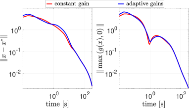
Figure 1: Results of Algorithms 3-3 for velocity-actuated vehicles.

We consider a connectivity problem formulated as a game, as in Stankovic et al. (2012). A group $\mathcal{I}=\{1,\dots,N=5\}$ of mobile sensor devices have to coordinate their actions via wireless communication, to perform some task, e.g., exploration or surveillance. Mathematically, each sensor $i$ aims at autonomously finding the position $x_{i}=\mathrm{col}(p^{x}_{i},p^{y}_{i})$ in a plane to optimize some private primary objective $c_{i}(x_{i})$, but not rolling away too much from the other devices. This goal is represented by the following cost functions, for all $i\in\mathcal{I}$:

$$\textstyle J_{i}\left(x_{i},x_{-i}\right):=c_{i}(x_{i})+\sum_{j\in\mathcal{I}}\left\|x_{i}-x_{j}\right\|^{2}.$$

Here, $c_{i}(x_{i}):=x_{i}^{T}x_{i}+d_{i}^{\top}x_{i}+{\sin(p^{x}_{i})}$, with $d_{i}\in\mathbb{R}^{2}$ randomly generated local parameters, for each $i\in\mathcal{I}$. The useful space is restricted by the local constraints $0.1\leq p^{y}_{i}\leq 0.5$, $\forall i\in\mathcal{I}$. The sensors communicate over a random undirected connected graph $\mathcal{G}(\mathcal{I},\mathcal{E})$. To preserve connectivity, the Chebyschev distance between any two neighboring agents has to be smaller than $\frac{1}{5}$, resulting in the coupling constraints $\max\{|p^{x}_{i}-p^{x}_{j}|,|p^{y}_{i}-p^{y}_{j}|\}\leq\frac{1}{5},\forall(i,j)\in\mathcal{E}$. After the deployment, all the sensors start sending the data they collect to a base station, located at $\bar{x}=\mathrm{col}(0,0.3)$, via wireless communication. To maintain acceptable levels of transmission power consumption, the average steady state distance from the base is limited as $\textstyle\frac{1}{N}\sum_{j\in\mathcal{N}_{i}}(x_{i}-\bar{x})^{\top}(x_{i}-\bar{x})\leq\frac{1}{2}$. This setup satisfies Assumptions 1-2. We set $c=30$ to satisfy the condition in Theorem 2; $\gamma_{i}=1,\forall i\in\mathcal{I}$; initial conditions are chosen randomly. We consider two different cases for the sensor physical dynamics.

Velocity-actuated vehicles: Each agent is a single-integrator as in (5). Figure 1 compares the results for Algorithms 3 and 3 (in logarithmic scale) and shows convergence of both to the unique v-GNE and asymptotic satisfaction of the coupling constraints. In the first phase, the controllers are mostly driven by the consensual dynamics; we remark that, when the agents agree on their estimates, the two algorithms coincide.

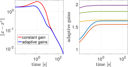
Figure 2: Results of Algorithm 6 for Euler–Lagrangian vehicles linearized via feedback linearization.

Euler–Lagrangian vehicles: Each mobile sensor $i\in\mathcal{I}$ is modeled as an Euler–Lagrangian systems of the form $I_{i}(x_{i})\ddot{x}_{i}+C_{i}(x_{i},\dot{x}_{i})+U_{i}(x_{i})=u_{i}$, where $U_{i}=\mathrm{col}(0,-1)$,

$$I_{i}(x_{i}) =\left[\begin{smallmatrix}2+0.6*\cos(p_{i}^{y})&0.5+0.3\cos(p_{i}^{y})\\ 0.5+0.3\cos(p_{i}^{y})&0.5\end{smallmatrix}\right],\$$

$$C_{i}(x_{i},\dot{x}_{i}) =\left[\begin{smallmatrix}-0.3\sin(p_{i}^{y})\dot{p}_{i}^{y}&-0.3\sin(p_{i}^{y})(\dot{p}_{i}^{x}+\dot{p}_{i}^{y})\\ 0.3\sin(p_{i}^{y})\dot{p}_{i}^{x}&0\end{smallmatrix}\right].$$

The systems satisfy the conditions in Remark 4 with uniform vector relative degree $\{2,2\}$. Therefore, we first apply a linearizing feedback; the problem then reduces to the control of double-integrator agents, and we choose the transformed input (see Remark 4) according to Algorithm 6 and the analogous algorithm with constant gain (obtained by choosing $\tilde{u}_{i}$ in (25a) according to Algorithm 3). The local constraints are dualized as in Remark 2. The results are illustrated in Figure 2. Finally, in Figure 3, we compare the trajectories of the vehicles in the velocity-actuated and Euler–Lagrangian cases. Importantly, the local constraints are satisfied along the whole trajectory for single-integrator agents, only asymptotically for the higher-order agents.

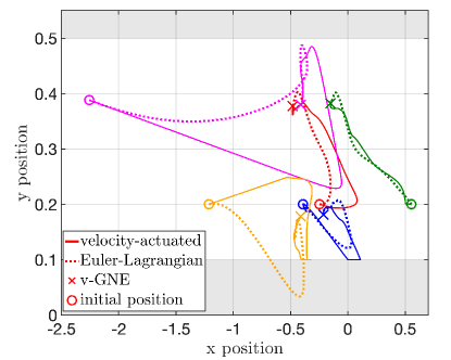
Figure 3: Cartesian trajectories of velocity-actuated and Euler–Lagrangian vehicles, with adaptive gains.

7.2 Competition in power markets as aggregative game

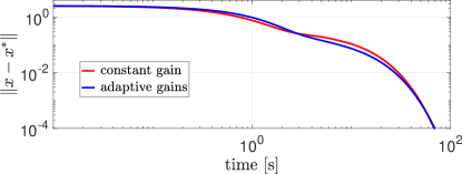
Figure 4: Distance from the v-GNE, for the power production in the electricity market.

We consider a Cournot competition model (Hobbs and Pang, 2007; Pavel, 2020). A group $\mathcal{I}=\{1,\dots,N\}$ of firms produces energy for a set of markets $\mathcal{J}=\{1,\dots,m\}$, each corresponding to a different location. Each firm $i\in\mathcal{I}$ controls a production plant in $n_{i}\leq m$ of the locations, and decides on the power outputs $x_{i}\in\mathbb{R}^{n_{i}}$ of its generators. Power is only dispatched in the location of production. Each plant has a maximal capacity, described by the local constraints $\boldsymbol{0}_{n_{i}}\leq x_{i}\leq X_{i}$. Moreover, an independednt system operator (ISO) imposes an upper bound on the market share of the producers, so that ${\boldsymbol{1}}_{n_{i}}^{\top}x_{i}\leq C_{i}$. Market clearance is guaranteed by the ISO via external control mechanisms, but the overall power generation is bounded by markets capacities $r=\mathrm{col}((r_{j})_{j\in\mathcal{J}})$. Thus, the firms share the constraints $Ax\leq r$. Here, $A=[A_{1}\dots A_{N}]$, and $A_{i}\in\mathbb{R}^{m\times n_{i}}$ with $[A_{i}]_{j,k}=1$ if $[x_{i}]_{k}$ is the power generated in location $j\in\mathcal{J}$ by agent $i$, $[A_{i}]_{j,k}=0$ otherwise, for all $j\in\mathcal{J}$, $k=1,\dots,n_{i}$. In simple terms, $Ax\in\mathbb{R}^{m}$ is the vector of total power generations for each market. Each firm $i\in\mathcal{I}$ aims at maximizing its profit, i.e., minimizing the cost

$$J_{i}(x_{i},x_{-i})=c_{i}(x_{i})-p(Ax)^{\top}A_{i}x_{i}+w({\boldsymbol{1}}_{n_{i}}^{\top}x_{i}),$$

where $c_{i}(x_{i})=\textstyle\sum_{k=1}^{n_{i}}Q_{i,k}([x_{i}]_{k})^{2}+q_{i,k}[x_{i}]_{k}$ is the generation cost, $p(Ax)^{\top}A_{i}x_{i}$ is the revenue, where $p:\mathbb{R}^{m}\rightarrow\mathbb{R}^{m}$ associates to each market a unitary price depending on the offer and $[p(Ax)]_{j}=P_{j}-\chi_{j}[Ax]_{j}$, $w(y)=w_{2}y-w_{1}y^{2}$ is a price charged by the ISO for the use of the infrastructure. We set $N=20$, $m=7$ and randomly select which firms participate in each market. We choose with uniform distribution $X_{i}$ in $[0.3,1.3]$, $C_{i}$ in $[1,2]$, $r_{j}$ in $[1,2]$, $Q_{i,k}$ in $[8,16]$, $q_{i}$ in $[1,2]$, ${P}_{j}$ in $[10,20]$, $\chi_{j}$ in $[1,3]$, for all $i\in\mathcal{I}$, $j\in\mathcal{J}$, $k=1,\dots,n_{i}$, $w_{1}$ in $[0.5,1]$, $w_{2}$ in $[0,0.1]$. The firms cannot access the productions of all the competitors, but can communicate with some neighbors on a connected graph. The turbine of generator $i$ is governed by the dynamics (Deng and Liang, 2019)

$$\dot{P}_{i,k} =\textstyle-\alpha^{1}_{i,k}P_{i,k}+\alpha^{2}_{i,k}R_{i,k}$$

$$\dot{R}_{i,k} =-\alpha^{3}_{i,k}R_{i,k}+\alpha^{4}_{i,k}u_{i,k},$$

with $P_{i,k}=[x_{i}]_{k}$; $R_{i,k}$ and $u_{i,k}$ are the steam valve opening and control input; the parameters $\alpha^{\cdot}_{i,k}$’s are set as in Deng and Liang (2019). Via feedback linearization, the problem for each generator reduces to the control of a double-integrator. The competition among the firms is described as an aggregative game with aggregation value $\psi(x)=Ax$ (this is advantageous with respect to the formulation in Pavel (2020), as the firms only keep an estimate of the aggregation and firm $i$ does not need to know the quantities $A_{j}$, $j\neq i$). We numerically check that this setup satisfies Assumptions 2, 4. We simulate the equivalent of Algorithm 6 for aggregative games, obtained by choosing $\tilde{u}_{i}$ in (25) according to Algorithms 5, 5; we deal with the local constraints as in Remark 2. The results are shown in Figure 4 and indicate fast convergence of the firms’ production to the unique v-GNE.

8 Conclusion and outlook

Generalized games played by nonlinear systems with maximal relative degree can be solved via continuous-time fully distributed primal-dual pseudogradient controllers, provided that the game mapping is strongly monotone and Lipschitz continuous. Convergence can be ensured even without a-priori knowledge on the game parameters, via integral consensus. Seeking an equilibrium when the agents are characterized by constrained dynamics is currently an open problem. The extension of our results to the case of direct communication, noise and parameter uncertainties is left as future work.

Appendix A Proof of Lemma 2

Under Assumption 3, we have, for any $q>0$,

$$\operatorname{Range}\left(\boldsymbol{L}_{q}\right) =\operatorname{Null}\left({\boldsymbol{1}}_{N}^{\top}\otimes I_{q}\right) =\boldsymbol{E}_{q}^{\perp},$$ (26)

$$\operatorname{Null}\left(\boldsymbol{L}_{q}\right) =\operatorname{Range}\left({\boldsymbol{1}}_{N}\otimes I_{q}\right) =\boldsymbol{E}_{q}.$$ (27)

i) For any equilibrium $\operatorname{col}({\bar{\boldsymbol{x}}},\boldsymbol{\bar{k}},{\bar{\boldsymbol{z}}},{\boldsymbol{\bar{\lambda}}})$ of (10), with $\boldsymbol{\bar{z}}\in\boldsymbol{E}^{\perp}_{m}$, it holds that

$$\boldsymbol{0} \in\mathcal{R}^{\top}\!(\boldsymbol{F}(\bar{\boldsymbol{x}})+\mathbb{G}(\mathcal{R}\boldsymbol{\bar{x}})^{\top}\boldsymbol{\bar{\lambda}}+\mathrm{N}_{\Omega}(\mathcal{R}\bar{\boldsymbol{x}}))\!+\!\boldsymbol{L}_{n}\bar{K}\boldsymbol{\bar{\rho}}$$ (28)

$$\boldsymbol{0} =D\left(\bar{\boldsymbol{\rho}}\right)^{\top}\left(\Gamma\otimes I_{n}\right)\bar{\boldsymbol{\rho}},\quad{\bar{\boldsymbol{\rho}}}=\boldsymbol{L}_{n}\bar{\boldsymbol{x}}$$ (29)

$$\boldsymbol{0} =\boldsymbol{L}_{m}\boldsymbol{\bar{\lambda}}$$ (30)

$$\boldsymbol{0} \in-\boldsymbol{g}(\mathcal{R}\boldsymbol{\bar{x}})+\boldsymbol{\bar{z}}+\boldsymbol{L}_{m}\boldsymbol{\bar{\lambda}}+\mathrm{N}_{\mathbb{R}_{\geq 0}^{Nm}}\left(\boldsymbol{\bar{\lambda}}\right),$$ (31)

where $\bar{K}=\operatorname{diag}((\bar{k}_{i}I_{n})_{i\in\mathcal{I}})$. By (29) we have $\bar{\boldsymbol{\rho}}=\boldsymbol{0}_{Nn}$, i.e., $\bar{\boldsymbol{x}}\in\boldsymbol{E}_{n}$ by (27), and by (30) and (27), we have $\bar{\boldsymbol{\lambda}}\in\boldsymbol{E}_{m}$. Hence, $\bar{\boldsymbol{x}}={\boldsymbol{1}}_{N}\otimes x^{*}$ and $\boldsymbol{\bar{\lambda}}={\boldsymbol{1}}_{N}\otimes\lambda^{*}$, for some $x^{*}\in\mathbb{R}^{n}$, $\lambda^{*}\in\mathbb{R}^{m}$. By left multiplying both sides of (28) by $({\boldsymbol{1}}_{N}^{\top}\otimes I_{n})$, by (27) and since $({\boldsymbol{1}}_{N}^{\top}\otimes I_{n})\mathcal{R}^{\top}=I_{n}$, $\boldsymbol{F}({{\boldsymbol{1}}_{N}\otimes x^{*}})=F(x^{*})$, $\mathcal{R}\bar{\boldsymbol{x}}=x^{*}$, and $\mathbb{G}(\mathcal{R}\boldsymbol{\bar{x}})^{\top}({\boldsymbol{1}}_{N}\otimes\lambda^{*})=\textstyle\frac{\partial}{\partial x}g(x^{*})^{\top}\lambda^{*}$, we retrieve the first KKT condition in (3). We obtain the second condition in (3) by left multiplying both sides of (31) by $({\boldsymbol{1}}_{N}^{\top}\otimes I_{m})$ and by using that $({\boldsymbol{1}}_{N}^{\top}\otimes I_{m})\boldsymbol{g}(\mathcal{R}\boldsymbol{\bar{x}})=g(x^{*})$, $({\boldsymbol{1}}_{N}^{\top}\otimes I_{m})\boldsymbol{\bar{z}}=0$ and $\textstyle{({\boldsymbol{1}}_{N}^{\top}\otimes I_{m})\mathrm{N}_{\mathbb{R}_{\geq 0}^{Nm}}({\boldsymbol{1}}_{N}\otimes\lambda^{*})=N\mathrm{N}_{\mathbb{R}_{\geq 0}^{m}}(\lambda^{*})=\mathrm{N}_{\mathbb{R}_{\geq 0}^{m}}(\lambda^{*})}$.

ii) Let $(x^{*},\lambda^{*})$ be any pair that satisfies the KKT conditions in (3). By taking $\bar{\boldsymbol{x}}={\boldsymbol{1}}_{N}\otimes x^{*}$, $\bar{\boldsymbol{\lambda}}={\boldsymbol{1}}_{N}\otimes\lambda^{*}$ and any $\bar{\boldsymbol{k}}$, (28)-(30) are satisfied as above. It suffices to show that there exists $\boldsymbol{\bar{z}}\in\boldsymbol{E}_{m}^{\perp}$ such that (31) holds, i.e., that $(-\boldsymbol{g}(\mathcal{R}\boldsymbol{\bar{x}})+\bar{v})\in\boldsymbol{E}_{m}^{\perp}$, for some $\bar{v}\in\mathrm{N}_{\mathbb{R}_{\geq 0}^{Nm}}(\boldsymbol{\bar{\lambda}})$. By (3), there exists $v^{*}\in\mathrm{N}_{\mathbb{R}^{m}_{\geq 0}}(\lambda^{*})$ such that $g(x^{*})=v^{*}$. Since $\mathrm{N}_{\mathbb{R}_{\geq 0}^{Nm}}({\boldsymbol{1}}_{N}\otimes\lambda^{*})=\times_{i\in\mathcal{I}}\mathrm{N}_{\mathbb{R}^{m}_{\geq 0}}(\lambda^{*})$, it follows by properties of cones that $\operatorname{col}(v_{1}^{*},\dots,v_{N}^{*})\in\mathrm{N}_{\mathbb{R}_{\geq 0}^{Nm}}(\boldsymbol{\bar{\lambda}})$ with $v_{1}^{*}=\dots=v_{N}^{*}=\frac{1}{N}v^{*}$. Therefore, $({\boldsymbol{1}}_{N}^{\top}\otimes I_{m})(-\boldsymbol{g}(\mathcal{R}\boldsymbol{\bar{x}})+\bar{v})=-g(x^{*})+v^{*}=\boldsymbol{0}_{m}$, or $(-\boldsymbol{g}(\mathcal{R}\boldsymbol{\bar{x}})+\bar{v})\in\boldsymbol{E}_{m}^{\perp}$. $\blacksquare$

Appendix B Proof of Lemma 4

Let $\boldsymbol{y}={\boldsymbol{1}}_{n}\otimes y$, for some $y\in\mathbb{R}^{n}$. We decompose $\boldsymbol{x}=\boldsymbol{x}^{\perp}+\boldsymbol{x}^{\parallel}$, where $\boldsymbol{x}^{\parallel}:=P_{n}\boldsymbol{x}$, $\boldsymbol{x}^{\perp}:=P^{\perp}_{n}\boldsymbol{x}$. Therefore, $\boldsymbol{x}^{\parallel}={\boldsymbol{1}}_{N}\otimes\hat{x}$, for some $\hat{x}\in\mathbb{R}^{n}$. By (Pavel, 2020, Eq. 50),

$$\begin{multlined}(\boldsymbol{x}-{\boldsymbol{y}})^{\top}\mathcal{R}^{\top}(\boldsymbol{F}(\boldsymbol{x})-\boldsymbol{F}(\boldsymbol{y}))\geq-\theta\|\hat{x}-y\|\|\boldsymbol{x}^{\perp}\|\\ +\mu\|\hat{x}-y\|^{2}-\theta\|\boldsymbol{x}^{\perp}\|^{2}-\theta_{0}\|\boldsymbol{x}^{\perp}\|\|\hat{x}-y\|.\end{multlined}(\boldsymbol{x}-{\boldsymbol{y}})^{\top}\mathcal{R}^{\top}(\boldsymbol{F}(\boldsymbol{x})-\boldsymbol{F}(\boldsymbol{y}))\geq-\theta\|\hat{x}-y\|\|\boldsymbol{x}^{\perp}\|\\ +\mu\|\hat{x}-y\|^{2}-\theta\|\boldsymbol{x}^{\perp}\|^{2}-\theta_{0}\|\boldsymbol{x}^{\perp}\|\|\hat{x}-y\|.$$

For any $k^{*}>\underline{k}>0$, we have $K^{*}\succ 0$ and, by (27), $\operatorname{Null}\left(\boldsymbol{L}_{n}K^{*}\boldsymbol{L}_{n}\right)=\boldsymbol{E}_{n}$. Therefore it holds that $(\boldsymbol{x}-\boldsymbol{y})^{\top}\boldsymbol{L}_{n}K^{*}\boldsymbol{L}_{n}(\boldsymbol{x}-\boldsymbol{y})\geq k^{*}\lambda_{2}(L)^{2}\|\boldsymbol{x}^{\perp}\|^{2}.$ By $\left\|\hat{x}-y\right\|=\textstyle\frac{1}{\sqrt{N}}\left\|\boldsymbol{x}^{\|}-\boldsymbol{y}\right\|$, we conclude that

$$\quad\ \left(\boldsymbol{x}-\boldsymbol{y}\right)^{\top}(\mathcal{R}^{\top}\left(\boldsymbol{F}(\boldsymbol{x})-\boldsymbol{F}\left(\boldsymbol{y}\right)\right)+\boldsymbol{L}_{n}K^{*}\boldsymbol{L}_{n}\left(\boldsymbol{x}-\boldsymbol{y}\right))$$

$$\geq\mathrm{col}(\|\boldsymbol{x}^{\perp}\|,\|\boldsymbol{x}^{\|}-\boldsymbol{y}\|)^{\top}M_{1}\mathrm{col}(\|\boldsymbol{x}^{\perp}\|,\|\boldsymbol{x}^{\|}-\boldsymbol{y}\|),$$

with ${M}_{1}$ as in (11) and, for $k^{*}>\underline{k}$, ${M}_{1}\succ 0$ by Silvester’s criterion. The conclusion follows since, by orthogonality, $\|\boldsymbol{x}^{\|}-\boldsymbol{y}\|^{2}+\|\boldsymbol{x}^{\perp}\|^{2}=\|\boldsymbol{x}-\boldsymbol{y}\|^{2}$. $\blacksquare$

Appendix C Proof of Theorem 1

We first rewrite the dynamics in (10) as

$$\dot{\boldsymbol{\omega}}=\Pi_{\Xi}({\boldsymbol{\omega}},-\mathcal{A}(\boldsymbol{\omega})-\mathcal{B}(\boldsymbol{\omega})),$$ (32)

where ${\boldsymbol{\omega}}:=\operatorname{col}\left({\boldsymbol{x}},{\boldsymbol{k}},{\boldsymbol{z}},{\boldsymbol{\lambda}}\right)$, $\Xi:=\boldsymbol{\Omega}\times\mathbb{R}^{N}\times\mathbb{R}^{Nm}\times\mathbb{R}^{mN}_{\geq 0}$,

$$\mathcal{A}(\boldsymbol{\omega}):=\left[\begin{smallmatrix}\mathcal{R}^{\top}\boldsymbol{F}(\boldsymbol{x})+\boldsymbol{L}_{n}K\boldsymbol{L}_{n}\boldsymbol{x}\\ -D({\boldsymbol{\rho}})^{\top}\left(\Gamma\otimes I_{n}\right){\boldsymbol{\rho}}\\ \boldsymbol{0}_{Nm}\\ \boldsymbol{L}_{m}\boldsymbol{\lambda}\end{smallmatrix}\right],\ \mathcal{B}(\boldsymbol{\omega}):=\left[\begin{smallmatrix}{{\mathcal{R}^{\top}\mathbb{G}(\mathcal{R}\boldsymbol{x})^{\top}}\boldsymbol{\lambda}}\\ \boldsymbol{0}_{N}\\ -\boldsymbol{L_{m}}\boldsymbol{\lambda}\\ {-\boldsymbol{g}(\mathcal{R}\boldsymbol{x})+\boldsymbol{z}}\end{smallmatrix}\right].$$

By Assumption 1 and Lemma 3, $\mathcal{A}$ and $\mathcal{B}$ are locally Lipschitz; therefore, for any initial condition in $\Xi$, the system (32) has a unique local Carathéodory solution, contained in $\Xi$ (Cherukuri et al., 2016). Moreover, we note that the set $S=\{\boldsymbol{w}\in\Xi\mid\boldsymbol{z}\in\boldsymbol{E}^{\perp}_{m}\}$ is invariant for the system (32), since for all $\boldsymbol{\omega}\in\Xi$, $\textstyle\frac{\partial}{\partial\boldsymbol{\omega}}(({\boldsymbol{1}}_{N}\otimes I_{m})^{\top}\boldsymbol{z})\dot{\boldsymbol{\omega}}=({\boldsymbol{1}}_{N}^{\top}\otimes I_{m})\boldsymbol{L}_{m}\boldsymbol{\lambda}=\boldsymbol{0}_{m}$.

Let $\Phi:=P_{m}+\boldsymbol{L}^{+}_{m}$, where $\boldsymbol{L}^{+}_{m}$ is the Moore-Penrose pseudo-inverse of $\boldsymbol{L}_{m}$, and we recall that $P_{m}=\textstyle\frac{1}{N}{\boldsymbol{1}}_{N}{\boldsymbol{1}}_{N}^{\top}\otimes I_{m}$ is the projection matrix on $\boldsymbol{E}_{m}$. By properties of the pseudo-inverse and (27), $\boldsymbol{L}^{+}_{m}={\boldsymbol{L}^{+}_{m}}^{\top}$, $\boldsymbol{L}^{+}_{m}\succeq 0$ and $\operatorname{Null}(\boldsymbol{L}^{+}_{m})=\boldsymbol{E}_{m}$. Since $\operatorname{Null}(P{{}_{m}})=\boldsymbol{E}_{m}^{\perp}$ and $P_{m}\succeq 0$, we have $\Phi\succ 0$. Also, $\boldsymbol{L}^{+}_{m}\boldsymbol{L}_{m}=I_{Nm}-P_{m}=P^{\perp}_{m}$ is the projector matrix on $\operatorname{Range}(\boldsymbol{L}_{m})=\boldsymbol{E}^{\perp}_{m}$. We define the quadratic Lyapunov function

$$V =\textstyle\frac{1}{2}\|\boldsymbol{\omega}-\bar{\boldsymbol{\omega}}\|^{2}_{Q}:=(\boldsymbol{\omega}-\bar{\boldsymbol{\omega}})^{\top}Q(\boldsymbol{\omega}-\bar{\boldsymbol{\omega}})$$

$$=\textstyle\frac{1}{2}(\|\boldsymbol{x}-\bar{\boldsymbol{x}}\|^{2}+\|\boldsymbol{k}-\boldsymbol{\bar{k}}\|^{2}_{\Gamma^{-1}}+\|\boldsymbol{z}-\boldsymbol{\bar{z}}\|_{{\Phi}}^{2}+\|\boldsymbol{\lambda}-\boldsymbol{\bar{\lambda}}\|^{2}),$$

where $Q=:\operatorname{diag}(I_{Nn},\Gamma^{-1},{\Phi},I_{Nm})$, and $\bar{\boldsymbol{x}}={\boldsymbol{1}}_{N}\otimes x^{*}$, $\bar{\boldsymbol{\lambda}}={\boldsymbol{1}}_{N}\otimes\lambda^{*}$, where the pair $(x^{*},\lambda^{*})$ satisfies the KKT conditions in (3), $\bar{\boldsymbol{k}}$ such that $k^{*}:=\min(\bar{\boldsymbol{k}})\geq\underline{k}$, with $\underline{k}$ as in (11), $\bar{\boldsymbol{z}}\in\boldsymbol{E}^{\perp}_{m}$ chosen such that $\bar{\boldsymbol{\omega}}:=\operatorname{col}\left(\bar{\boldsymbol{x}},\bar{\boldsymbol{k}},\bar{\boldsymbol{z}},\bar{\boldsymbol{\lambda}}\right)$ is an equilibrium for (10), and such a $\bar{\boldsymbol{z}}$ exists by the proof of Lemma 2. Therefore, for any $\boldsymbol{\omega}\in S$, we have

$$\dot{V}(\boldsymbol{\omega}): =\nabla V(\boldsymbol{\omega})\dot{\boldsymbol{\omega}}=(\boldsymbol{\omega}-\bar{\boldsymbol{\omega}})^{\top}Q\dot{\boldsymbol{\omega}}=$$

$$=(\boldsymbol{\omega}-\bar{\boldsymbol{\omega}})^{\top}Q\Pi_{\Xi}({\boldsymbol{\omega}},-\mathcal{A}(\boldsymbol{\omega})-\mathcal{B}(\boldsymbol{\omega}))$$

$$\leq(\boldsymbol{\omega}-\bar{\boldsymbol{\omega}})^{\top}Q(-\mathcal{A}(\boldsymbol{\omega})-\mathcal{B}(\boldsymbol{\omega})),$$ (33)

where the last inequality follows from Lemma 1 and by exploiting the structure of $Q$ and $\Xi$. By Lemma 1, it also holds that $(\boldsymbol{\omega}-\bar{\boldsymbol{\omega}})^{\top}Q(-\mathcal{A}(\bar{\boldsymbol{\omega}})-\mathcal{B}(\bar{\boldsymbol{\omega}}))\leq 0.$ By subtracting this term from (33), we obtain

$$\dot{V}(\boldsymbol{\omega})\leq-(\boldsymbol{\omega}-\boldsymbol{\bar{\omega}})^{\top}Q(\mathcal{A}(\boldsymbol{\omega})-\mathcal{A}(\boldsymbol{\bar{\omega}})+\mathcal{B}(\boldsymbol{\omega})-\mathcal{B}(\boldsymbol{\bar{\omega}})).$$

Besides, for any $\boldsymbol{z}\in\boldsymbol{E}^{\perp}_{m}$, by $\boldsymbol{L}^{+}_{m}\boldsymbol{L}_{m}=P^{\perp}_{m}$ and (27), we have $(\boldsymbol{z}-\boldsymbol{\bar{z}})^{\top}\Phi\boldsymbol{L}_{m}(\boldsymbol{\lambda}-\bar{\boldsymbol{\lambda}})=(\boldsymbol{z}-\boldsymbol{\bar{z}})^{\top}(\boldsymbol{\lambda}-\bar{\boldsymbol{\lambda}})$, and hence

$$\quad\ (\boldsymbol{\omega}-\boldsymbol{\bar{\omega}})^{\top}Q(\mathcal{B}(\boldsymbol{\omega})-\mathcal{B}(\boldsymbol{\bar{\omega}}))$$

$$=(\boldsymbol{x}-\bar{\boldsymbol{x}})^{\top}\mathcal{R}^{\top}(\mathbb{G}(\mathcal{R}\boldsymbol{x})^{\top}\boldsymbol{\lambda}-{\mathbb{G}(\mathcal{R}\bar{\boldsymbol{x}})^{\top}}\bar{\boldsymbol{\lambda}})$$

$$\quad\ +(\boldsymbol{\lambda}-\bar{\boldsymbol{\lambda}})^{\top}(-\boldsymbol{g}(\mathcal{R}\boldsymbol{x})+\boldsymbol{g}(\mathcal{R}\bar{\boldsymbol{x}}))$$

$$=(x-x^{*})^{\top}(\nabla_{\!\!y}(\boldsymbol{g}(y)^{\top}\boldsymbol{\lambda})|_{y=x}-\nabla_{\!\!y}(\boldsymbol{g}(y)^{\top}\boldsymbol{\bar{\lambda}})|_{y=x^{*}})$$

$$\quad\ -(\boldsymbol{\lambda}-\boldsymbol{\bar{\lambda}})^{\top}(\nabla_{\!\!y}(\boldsymbol{g}(x)^{\top}y)|_{y=\boldsymbol{\lambda}}-\nabla_{\!\!y}(\boldsymbol{g}(x^{*})^{\top}y)|_{y=\bar{\boldsymbol{\lambda}}})\geq 0$$

and the last inequality holds, for any $\boldsymbol{\omega}\in S$, by applying (Rockafellar, 1970, Th. 1) (since $\boldsymbol{\lambda},\boldsymbol{\bar{\lambda}}\in\mathbb{R}_{\geq 0}^{Nm}$ and by Assumption 1). Therefore, for any $\boldsymbol{\omega}\in S$, it holds that:

$$\dot{V}(\boldsymbol{\omega}) \leq-(\boldsymbol{\omega}-\boldsymbol{\bar{\omega}})^{\top}Q\left(\mathcal{A}(\boldsymbol{\omega})-\mathcal{A}(\boldsymbol{\bar{\omega}})\right)$$

$$\begin{aligned} &=-(\boldsymbol{x}-\bar{\boldsymbol{x}})^{\top}\mathcal{R}^{\top}\left(\boldsymbol{F}(\boldsymbol{x})-\boldsymbol{F}(\boldsymbol{\bar{x}})\right)\\ &\quad-(\boldsymbol{x}-\bar{\boldsymbol{x}})^{\top}(\boldsymbol{L}_{n}K\boldsymbol{L}_{n}(\boldsymbol{x}-\bar{\boldsymbol{x}}))\\ &\quad+(\boldsymbol{k}-\bar{\boldsymbol{k}})^{\top}\Gamma^{-1}D({\boldsymbol{\rho}})^{\top}\left(\Gamma\otimes I_{n}\right){\boldsymbol{\rho}}\\ &\quad-(\boldsymbol{\lambda}-\bar{\boldsymbol{\lambda}})^{\top}\boldsymbol{L}_{m}(\boldsymbol{\lambda}-\bar{\boldsymbol{\lambda}}),\end{aligned}$$ (34)

where we used that $\bar{\boldsymbol{\rho}}:=\boldsymbol{L}_{n}\bar{\boldsymbol{x}}=0$. For the last addend in (34), we can write $(\boldsymbol{\lambda}-\bar{\boldsymbol{\lambda}})^{\top}\boldsymbol{L}_{m}(\boldsymbol{\lambda}-\bar{\boldsymbol{\lambda}})=\boldsymbol{\lambda}^{\top}\boldsymbol{L}_{m}\boldsymbol{\lambda}$ by (27) and, by (Bauschke and Combettes, 2017, Th. $18.15$), $\boldsymbol{\lambda}^{\top}\boldsymbol{L}_{m}\boldsymbol{\lambda}\geq\frac{1}{2\uplambda_{\textnormal{max}}(L)}\|\boldsymbol{L}_{m}\boldsymbol{\lambda}\|^{2}$. The third addend in (34) can be rewritten as $(\boldsymbol{k}-\bar{\boldsymbol{k}})^{\top}\Gamma^{-1}D({\boldsymbol{\rho}})^{\top}\left(\Gamma\otimes I_{n}\right){\boldsymbol{\rho}}=\textstyle\sum_{i=1}^{N}\left(k_{i}-\bar{k}_{i}\right){\boldsymbol{\rho}}^{i\top}{\boldsymbol{\rho}}^{i}={\boldsymbol{\rho}}^{\top}(K-\bar{K}){\boldsymbol{\rho}}=\boldsymbol{x}^{\top}\boldsymbol{L}_{n}(K-\bar{K})\boldsymbol{L}_{n}\boldsymbol{x}=(\boldsymbol{x}-\bar{\boldsymbol{x}})^{\top}\boldsymbol{L}_{n}(K-\bar{K})\boldsymbol{L}_{n}(\boldsymbol{x}-\bar{\boldsymbol{x}}),$ where $\bar{K}:=\operatorname{diag}((\bar{k}_{i}I_{n})_{i\in\mathcal{I}})$. Therefore, the sum of the second and third term in (34) is $-(\boldsymbol{x}-\bar{\boldsymbol{x}})^{\top}\boldsymbol{L}_{n}\bar{K}\boldsymbol{L}_{n}(\boldsymbol{x}-\bar{\boldsymbol{x}})\leq-(\boldsymbol{x}-\bar{\boldsymbol{x}})^{\top}\boldsymbol{L}_{n}K^{*}\boldsymbol{L}_{n}(\boldsymbol{x}-\bar{\boldsymbol{x}})$, where $K^{*}:=k^{*}I_{Nn}$. By Lemma 4, we finally get

$$\dot{V}\leq-\uplambda_{\textnormal{min}}(M_{1})\|\boldsymbol{x}-\bar{\boldsymbol{x}}\|^{2}-\textstyle\frac{1}{2\uplambda_{\textnormal{max}}(L)}\|\boldsymbol{L}_{m}\boldsymbol{\lambda}\|^{2},$$ (35)

with $M_{1}\succ 0$ as in Lemma 4.

Let $\mathcal{\bar{P}}$ be any compact sublevel set of $V$ (notice that $V$ is radially unbounded) containing the initial condition $\boldsymbol{\omega}(0)\in S$. $\mathcal{\bar{P}}$ is invariant for the dynamics, since $\dot{V}(\boldsymbol{\omega})\leq 0$ by (35). The set $\mathcal{P}:=\mathcal{\bar{P}}\cap S$ is compact, convex and invariant, therefore, by exploiting Lemma 3 and the continuous differentiability in Assumption 1, we conclude that $\mathcal{A}+\mathcal{B}$ is Lipschitz continuous on $\mathcal{P}$. Therefore, for any initial condition, there exists a unique global Carathéodory solution to (10), that belongs to $\mathcal{P}$ (and therefore is bounded) for every $t$ (Cherukuri et al., 2016, Prop. $2.2$). Moreover, by (De Persis and Grammatico, 2019, Th. $2$), the solution converges to the largest invariant set $\mathcal{O}\subseteq\{\boldsymbol{\omega}\in\mathcal{P}\text{s.t.}\dot{V}(\boldsymbol{\omega})=0\}$.

We can already conclude that $\boldsymbol{x}$ converges to the point ${\boldsymbol{1}}_{N}\otimes x^{*}$, with $x^{*}$ the unique v-GNE of the game in (2). We next show convergence of the other variables. Take any point $\underline{\boldsymbol{\omega}}:=\operatorname{col}(\underline{\boldsymbol{x}},\underline{\boldsymbol{k}},\underline{\boldsymbol{z}},\underline{\boldsymbol{\lambda}})\in\mathcal{O}$. Since $\dot{V}(\underline{\boldsymbol{\omega}})=0$, by (35) we have $\underline{\boldsymbol{x}}=\boldsymbol{\bar{x}}={\boldsymbol{1}}_{N}\otimes x^{*},$ and $\underline{\boldsymbol{\lambda}}\in\boldsymbol{E}_{m}$, i.e. $\underline{\boldsymbol{\lambda}}={\boldsymbol{1}}_{N}\otimes\underline{\lambda}$, for some $\underline{\lambda}\in\mathbb{R}^{m}_{\geq 0}$. Therefore, by expanding (33), by $\underline{\boldsymbol{x}}=\bar{\boldsymbol{x}}$, $\underline{\boldsymbol{\rho}}:=\boldsymbol{L}_{n}\underline{\boldsymbol{x}}=\boldsymbol{0}_{Nn}$ and (27), we have

$$0 =(\boldsymbol{\underline{\lambda}}-\boldsymbol{\bar{\lambda}})^{\top}(\boldsymbol{g}(R\bar{\boldsymbol{x}})-{\boldsymbol{\underline{z}}})=(\underline{\lambda}-\lambda^{*})^{\top}g(x^{*})$$

$$=\underline{\lambda}^{\top}g(x^{*})=\boldsymbol{\underline{\lambda}}^{\top}(\boldsymbol{g}(\mathcal{R}\bar{\boldsymbol{x}}){-\boldsymbol{\underline{z}})}),$$ (36)

where in the second equality we have used that $\underline{\boldsymbol{z}}\in\boldsymbol{E}^{\perp}_{m}$  and the third equality follows from the KKT conditions in (3b). Then, let $\underline{\boldsymbol{\omega}}(t)=\operatorname{col}(\underline{\boldsymbol{x}}(t),\underline{\boldsymbol{k}}(t),\underline{\boldsymbol{z}}(t),\underline{\boldsymbol{\lambda}}(t))$ be the trajectory of (32) starting at $\underline{\boldsymbol{\omega}}$. By invariance of $\mathcal{O}$, $\underline{\boldsymbol{x}}(t)=\bar{\boldsymbol{x}}$ and $\underline{\lambda}(t)\in\boldsymbol{E}_{m}$, for all $t$. Therefore, by (10b)-(10c), it holds that ${\underline{\boldsymbol{k}}}(t)\equiv{\underline{\boldsymbol{k}}}$, $\underline{\boldsymbol{z}}(t)\equiv\underline{\boldsymbol{z}}$, for all $t$. Hence, the quantity $v:=(\boldsymbol{g}(\mathcal{R}\underline{\boldsymbol{x}}(t)){-\boldsymbol{L}_{m}\underline{\boldsymbol{\lambda}}(t)-\underline{\boldsymbol{z}}(t)})$ is a constant along the trajectory $\underline{\boldsymbol{\omega}}(t)$. Suppose by contradiction that $[v]_{k}>0$, for some $k=\{1,\dots,Nm\}$. Then, $[\dot{\underline{\boldsymbol{\lambda}}}(t)]_{k}=[v]_{k}$ for almost all $t$, by (10d), and ${\underline{\boldsymbol{\lambda}}}(t)$ grows indefinitely. Since all the solutions of (10) are bounded, this is a contradiction. Therefore, $v\leq\boldsymbol{0}_{m}$, and $\underline{\boldsymbol{\lambda}}^{\top}v=0$ by (36). Equivalently, $\textstyle v\in{N}_{\mathbb{R}_{\geq 0}^{Nm}}(\underline{\boldsymbol{\lambda}})$, hence ${\underline{\boldsymbol{\lambda}}}(t)\equiv\underline{\boldsymbol{\lambda}}$, for all $t$. We conclude that the points in $\mathcal{O}$ are equilibria.

Moreover, the set $\Lambda(\boldsymbol{\omega}_{0})$ of $\omega$-limit pointsof the solution to (10) starting at any $\boldsymbol{\omega}_{0}\in S$ is nonempty (by Bolzano-Weierstrass theorem, since all the trajectories of (10) are bounded), and $\Lambda(\boldsymbol{\omega}_{0})\subseteq\mathcal{O}$ (see the proof of (De Persis and Grammatico, 2019, Th.2)). Hence, all the $\omega$-limit points are equilibria. We next show that, for any for any $\boldsymbol{\omega}_{0}\in S$, $\Lambda(\boldsymbol{\omega}_{0})$ is a singleton; as a consequence, the solution converges to that point (Bauschke and Combettes, 2017, Lemma $1.14$). For the sake of contradiction, assume that there are two $\omega$-limit points $\boldsymbol{\omega}_{1}=\operatorname{col}({\bar{\boldsymbol{x}}},\hat{{\boldsymbol{k}}},{{\boldsymbol{z}}}_{1},{{\boldsymbol{\lambda}}}_{1})$, $\boldsymbol{\omega}_{2}=\operatorname{col}({\bar{\boldsymbol{x}}},\hat{{\boldsymbol{k}}},{{\boldsymbol{z}}}_{2},{{\boldsymbol{\lambda}}}_{2})\in\Lambda(\boldsymbol{\omega}_{0})$, with $\boldsymbol{\omega}_{1}\neq\boldsymbol{\omega}_{2}$. We note that $\boldsymbol{\omega}_{1}$ and $\boldsymbol{\omega}_{2}$ must have the same vector of adaptive gains $\hat{{\boldsymbol{k}}}$ by definition of $\omega$-limit point, since the $k_{i}$’s in Algorithm 3 are nonincreasing. Let $\boldsymbol{\omega}_{3}=\operatorname{col}({\bar{\boldsymbol{x}}},\hat{{\boldsymbol{k}}}+{\boldsymbol{1}}\alpha,{{\boldsymbol{z}}}_{1},{{\boldsymbol{\lambda}}}_{1})$, $\alpha\in\mathbb{R}$ chosen such that $\min(\hat{{\boldsymbol{k}}}+{\boldsymbol{1}}\alpha)>\underline{k}$, $\underline{k}$ as in (11). By (35), $\|\boldsymbol{\omega}(t)-\boldsymbol{\omega}_{3}\|_{Q}$ is nonincreasing along the trajectory $\boldsymbol{\omega}(t)$ of (32) starting at $\boldsymbol{\omega}_{0}$. Thus, by definition of $\omega$-limit point, it holds that $\|\boldsymbol{\omega}_{1}-\boldsymbol{\omega}_{3}\|_{Q}=\|\boldsymbol{\omega}_{2}-\boldsymbol{\omega}_{3}\|_{Q}$, or $\|\mathrm{col}(\boldsymbol{0}_{Nn},\alpha{\boldsymbol{1}}_{N},\boldsymbol{0}_{Nm},\boldsymbol{0}_{Nm})\|_{Q}=\|\mathrm{col}(\boldsymbol{0}_{Nn},\alpha{\boldsymbol{1}}_{N},{\boldsymbol{\lambda}}_{1}-{\boldsymbol{\lambda}}_{2},{{\boldsymbol{z}}}_{2}-{{\boldsymbol{z}}}_{1})\|_{Q}$. Equivalently, $\boldsymbol{\omega}_{1}=\boldsymbol{\omega}_{2}$, that is a contradiction. $\blacksquare$

Appendix D Proof of Theorem 2

The proof follows as for Theorem 1, by defining ${\boldsymbol{\omega}}:=\operatorname{col}\left({\boldsymbol{x}},{\boldsymbol{z}},{\boldsymbol{\lambda}}\right)$, $\Xi:=\boldsymbol{\Omega}\times\mathbb{R}^{Nm}\times\mathbb{R}^{mN}_{\geq 0}$,

$$\mathcal{A}(\boldsymbol{\omega}):=\left[\begin{smallmatrix}\mathcal{R}^{\top}\boldsymbol{F}(\boldsymbol{x})+c\boldsymbol{L}_{n}\boldsymbol{x}\\ \boldsymbol{0}_{Nm}\\ \boldsymbol{L}_{m}\boldsymbol{\lambda}\end{smallmatrix}\right],\ \mathcal{B}(\boldsymbol{\omega}):=\left[\begin{smallmatrix}{\mathcal{R}^{\top}\mathbb{G}(\mathcal{R}\boldsymbol{x})^{\top}}\boldsymbol{\lambda}\\ -\boldsymbol{L_{m}}\boldsymbol{\lambda}\\ -\boldsymbol{g}(\mathcal{R}\boldsymbol{x})+\boldsymbol{z}\end{smallmatrix}\right],$$

with Lyapunov function $V(\boldsymbol{\omega})=\textstyle\frac{1}{2}(\|\boldsymbol{x}-\bar{\boldsymbol{x}}\|^{2}+\|\boldsymbol{z}-\boldsymbol{\bar{z}}\|_{{\Phi}}^{2}+\|\boldsymbol{\lambda}-\boldsymbol{\bar{\lambda}}\|^{2})$, and by exploiting, in place of Lemma 4, Lemma 3 in Pavel (2020). $\blacksquare$

Appendix E Proof of Lemma 5

By Assumptions 2 and  4, we have

$$\quad\ (x-x^{\prime})^{\top}(\boldsymbol{\tilde{F}}(x,\boldsymbol{\sigma})-\boldsymbol{\tilde{F}}(x^{\prime},\boldsymbol{\sigma}^{\prime})$$

$$=\begin{multlined}(x-x^{\prime})^{\top}(\boldsymbol{\tilde{F}}(x,\boldsymbol{\sigma})-\boldsymbol{\tilde{F}}(x,P_{\bar{n}}{\boldsymbol{\psi}}(x))\\ ~{}~{}~{}~{}~{}~{}~{}~{}~{}~{}~{}~{}+\boldsymbol{\tilde{F}}(x,P_{\bar{n}}{\boldsymbol{\psi}}(x))-\boldsymbol{\tilde{F}}(x^{\prime},P_{\bar{n}}{\boldsymbol{\psi}}(x^{\prime})))\end{multlined}(x-x^{\prime})^{\top}(\boldsymbol{\tilde{F}}(x,\boldsymbol{\sigma})-\boldsymbol{\tilde{F}}(x,P_{\bar{n}}{\boldsymbol{\psi}}(x))\\ ~{}~{}~{}~{}~{}~{}~{}~{}~{}~{}~{}~{}+\boldsymbol{\tilde{F}}(x,P_{\bar{n}}{\boldsymbol{\psi}}(x))-\boldsymbol{\tilde{F}}(x^{\prime},P_{\bar{n}}{\boldsymbol{\psi}}(x^{\prime})))$$

$$\geq{\mu}\|x-x^{\prime}\|^{2}-\tilde{\theta}_{\sigma}\|x-x^{\prime}\|\|{\boldsymbol{\sigma}}-{\boldsymbol{1}}_{N}\otimes\psi(x)\|.$$

Moreover, we note that $(\boldsymbol{\sigma}-{\boldsymbol{1}}_{N}\otimes\psi(x))\in\boldsymbol{E}^{\perp}_{\bar{n}}$, since $P_{\bar{n}}\boldsymbol{\sigma}=P_{\bar{n}}{\boldsymbol{\psi}}(x)$, and ${\boldsymbol{\sigma}}^{\prime}\in\boldsymbol{E}_{\bar{n}}$. Hence, by (27), we have $(\boldsymbol{\sigma}-{\boldsymbol{\sigma}}^{\prime})^{\top}\boldsymbol{L}_{{\bar{n}}}K^{*}\boldsymbol{L}_{{\bar{n}}}(\boldsymbol{\sigma}-{\boldsymbol{\sigma}}^{\prime})\geq k^{*}\uplambda_{2}(L)^{2}\|\boldsymbol{\sigma}-P_{\bar{n}}{\boldsymbol{\psi}}(x)\|^{2},$ and the conclusion follows readily. $\blacksquare$

Appendix F Proof of Theorem 3

The dynamics (16) can be recast in the form (32), with ${\boldsymbol{\omega}}=\operatorname{col}\left(x,\boldsymbol{\varsigma},{\boldsymbol{k}},{\boldsymbol{z}},{\boldsymbol{\lambda}}\right)$, $\Xi=\Omega\times\mathbb{R}^{N{\bar{n}}}\times\mathbb{R}^{N}\times\mathbb{R}^{Nm}\times\mathbb{R}_{\geq 0}^{Nm}$,

$$\mathcal{A}(\boldsymbol{\omega})=\left[\begin{smallmatrix}\boldsymbol{\tilde{F}}(x,\boldsymbol{\sigma})+{B^{\top}}\boldsymbol{L}_{{\bar{n}}}K\boldsymbol{L}_{{\bar{n}}}\boldsymbol{\sigma}\\ \boldsymbol{L}_{{\bar{n}}}K\boldsymbol{L}_{{\bar{n}}}\boldsymbol{\sigma}\\ -D({\boldsymbol{\rho}})^{\top}\left(\Gamma\otimes I_{\bar{n}}\right){\boldsymbol{\rho}}\\ \boldsymbol{0}_{Nm}\\ \boldsymbol{L}_{m}\boldsymbol{\lambda}\end{smallmatrix}\right],\;\mathcal{B}(\boldsymbol{\omega})=\left[\begin{smallmatrix}\mathbb{G}(x)^{\top}\boldsymbol{\lambda}\\ \boldsymbol{0}_{N{\bar{n}}}\\ \boldsymbol{0}_{N}\\ -\boldsymbol{L}_{m}\boldsymbol{\lambda}\\ -\boldsymbol{g}(x)+\boldsymbol{z}\end{smallmatrix}\right].$$

By proceeding as in the proof of Theorem 1, we note that the set $S$ is invariant for the dynamics, since, for all $\boldsymbol{\omega}\in S$, $\textstyle\frac{\partial}{\partial\boldsymbol{\omega}}(P_{{\bar{n}}}\boldsymbol{\varsigma})\dot{{\boldsymbol{\omega}}}=\boldsymbol{0}_{N{\bar{n}}}$, $\textstyle\frac{\partial}{\partial\boldsymbol{\omega}}(P_{m}\boldsymbol{z})\dot{{\boldsymbol{\omega}}}=\boldsymbol{0}_{Nm}$.

Analogously to the proof of Lemma 2, it can be shown that any equilibrium point ${\bar{\boldsymbol{\omega}}}:=\operatorname{col}\left(\bar{x},\bar{\boldsymbol{\varsigma}},{\bar{\boldsymbol{k}}},{\bar{\boldsymbol{z}}},{\bar{\boldsymbol{\lambda}}}\right)\in S$ of (16) is such that $\bar{\boldsymbol{\lambda}}={\boldsymbol{1}}_{N}\otimes\lambda^{*}$, the pair $(\bar{x},\lambda^{*})$ satisfies the KKT conditions in (3), and $\bar{{\boldsymbol{\sigma}}}:={\boldsymbol{\psi}}(\bar{x})+\bar{\boldsymbol{\varsigma}}={\boldsymbol{1}}_{N}\otimes\psi(\bar{x})$. Moreover, for any pair $(x^{*},\lambda^{*})$ satisfying the KKT conditions in (3), there exists $\bar{\boldsymbol{z}}\in\mathbb{R}^{mN}$ such that $\operatorname{col}(x^{*},{{\boldsymbol{1}}_{N}\otimes\psi({x}^{*})-{\boldsymbol{\psi}}(x^{*})},\boldsymbol{k},\bar{\boldsymbol{z}},{\boldsymbol{1}}_{N}\otimes\lambda^{*})\in S$ is an equilibrium for (16), for any $\boldsymbol{k}\in\mathbb{R}^{N}$. The proof is omitted because of space limitations.

Let ${\bar{\boldsymbol{\omega}}}=\operatorname{col}\left(\bar{x},\bar{\boldsymbol{\varsigma}},{\bar{\boldsymbol{k}}},{\bar{\boldsymbol{z}}},{\bar{\boldsymbol{\lambda}}}\right)\in S$ be an equilibrium of (16) such that $k^{*}=\min(\bar{\boldsymbol{k}})>\underline{k}$, $\underline{k}$ as in (18), and consider the quadratic Lyapunov function $V=\textstyle\frac{1}{2}\|\boldsymbol{\omega}-\bar{\boldsymbol{\omega}}\|^{2}_{Q}$, where $Q=\operatorname{diag}(I_{n},I_{N{\bar{n}}},\Gamma^{-1},P_{m}+\boldsymbol{L}_{m}^{+},I_{Nm})$. Analogously to the proof of Theorem 2, it holds that $(\boldsymbol{\omega}-\boldsymbol{\bar{\omega}})^{\top}Q(\mathcal{B}(\boldsymbol{\omega})-\mathcal{B}(\boldsymbol{\bar{\omega}}))\geq 0$, and that $\dot{V}(\boldsymbol{\omega})\leq-(\boldsymbol{\omega}-\boldsymbol{\bar{\omega}})^{\top}Q\left(\mathcal{A}(\boldsymbol{\omega})-\mathcal{A}(\boldsymbol{\bar{\omega}})\right)$, for all $\boldsymbol{\omega}\in S$. Also we note that

$$(x-\bar{x})^{\top}B^{\top}\boldsymbol{L}_{{\bar{n}}}K\boldsymbol{L}_{{\bar{n}}}(\boldsymbol{\sigma}-\bar{\boldsymbol{\sigma}})+(\boldsymbol{\varsigma}-\bar{\boldsymbol{\varsigma}})^{\top}\boldsymbol{L}_{{\bar{n}}}K\boldsymbol{L}_{{\bar{n}}}(\boldsymbol{\sigma}-\bar{\boldsymbol{\sigma}})$$

$$=(\boldsymbol{\varsigma}+Bx+d-(\bar{\boldsymbol{\varsigma}}+B\bar{x}+d))^{\top}\boldsymbol{L}_{{\bar{n}}}K\boldsymbol{L}_{{\bar{n}}}(\boldsymbol{\sigma}-\bar{\boldsymbol{\sigma}})$$

$$=(\boldsymbol{\sigma}-\bar{\boldsymbol{\sigma}})^{\top}\boldsymbol{L}_{{\bar{n}}}K\boldsymbol{L}_{{\bar{n}}}(\boldsymbol{\sigma}-\bar{\boldsymbol{\sigma}}),$$

where $d:=\mathrm{col}((d_{i})_{i\in\mathcal{I}}))$, and that $(\boldsymbol{k}-\bar{\boldsymbol{k}})^{\top}\Gamma^{-1}D({\boldsymbol{\rho}})^{\top}(\Gamma\otimes I_{n}){\boldsymbol{\rho}}=(\boldsymbol{\sigma}-\bar{\boldsymbol{\sigma}})^{\top}\boldsymbol{L}_{n}(K-\bar{K})\boldsymbol{L}_{n}(\boldsymbol{\sigma}-\bar{\boldsymbol{\sigma}})$ as in the proof of Theorem 2. Hence, by Lemma 5, we obtain, for all $\boldsymbol{\omega}\in S$

$$\begin{multlined}\dot{V}(\boldsymbol{\omega})\leq-\uplambda_{\textnormal{min}}(M_{2})(\|x-{\bar{x}}\|^{2}+\|\boldsymbol{\sigma}-{\boldsymbol{1}}_{N}\otimes\psi(x)\|^{2})\\ -\textstyle\frac{1}{2\uplambda_{\textnormal{max}}(L)}\|\boldsymbol{L}_{m}\boldsymbol{\lambda}\|^{2},\end{multlined}\dot{V}(\boldsymbol{\omega})\leq-\uplambda_{\textnormal{min}}(M_{2})(\|x-{\bar{x}}\|^{2}+\|\boldsymbol{\sigma}-{\boldsymbol{1}}_{N}\otimes\psi(x)\|^{2})\\ -\textstyle\frac{1}{2\uplambda_{\textnormal{max}}(L)}\|\boldsymbol{L}_{m}\boldsymbol{\lambda}\|^{2},$$

with $M_{2}\succ 0$ as in (18). Then, existence of a unique global solution for the system in (16) and convergence to an equilibrium point follows as for Theorem 1. $\blacksquare$

Appendix G Proof of Theorem 4

Analogously to Lemma 5, it can be shown that for any $c>\underline{c}$, for any $(x,\boldsymbol{\sigma})$ such that $P_{{\bar{n}}}\boldsymbol{\sigma}=P_{{\bar{n}}}{\boldsymbol{\psi}}(x)$ and any $(x^{\prime},\boldsymbol{{\sigma}}^{\prime})$ such that ${\boldsymbol{\sigma}}^{\prime}=P_{{\bar{n}}}{\boldsymbol{\psi}}(x^{\prime})$, it holds that ${(x-x^{\prime})^{\top}(\boldsymbol{\tilde{F}}(x,{\boldsymbol{\sigma}})-\boldsymbol{\tilde{F}}(x^{\prime},{{\boldsymbol{\sigma}}^{\prime}}))}+{c({\boldsymbol{\sigma}}-{{\boldsymbol{\sigma}}^{\prime}})^{\top}\boldsymbol{L}_{{\bar{n}}}({\boldsymbol{\sigma}}-{{\boldsymbol{\sigma}}^{\prime}})}\allowbreak\geq\delta\|\mathrm{col}(x-x^{\prime},{\boldsymbol{\sigma}}-{{\boldsymbol{1}}_{N}\otimes\psi(x)})\|^{2}$, for some $\delta>0$. Then, the proof follows analogously to Theorem 3. $\blacksquare$

Appendix H Proof of Theorem 5

Under the coordinate transformations in (22), the dynamics in Algorithm 6 read as (25), where the input $\tilde{u}_{i}$ in Algorithm 6 has been chosen by design according to Algorithm 3, under Assumption 5. Therefore, existence of a unique bounded solution and convergence of ${\zeta}_{i}$ to $x_{i}^{*}$ (and of the variables $\boldsymbol{\zeta}^{i},k_{i},z_{i},\lambda_{i}$), for all $i\in\mathcal{I}$, follows from Theorem 1. On the other hand, we note that, for all $i\in\mathcal{I}$ and all $k\in\mathcal{M}_{i}$, $E_{i,k}$ is Hurwitz, because it is in canonical controllable form and the coefficients of the last row are by design the coefficients of an Hurwitz polynomial. Therefore, $E_{i}$ is also Hurwitz, and hence the dynamics in (25b) are ISS with respect to the input $\tilde{u}_{i}$ (Khalil, 2002, Lemma 4.6). In turn, the input $\tilde{u}_{i}$ is bounded, by boundedness of trajectories in Theorem 1, Assumption 1 and Lemma 3; moreover, by the convergence in Theorem 1, the KKT conditions in (3) and by continuity, we have that $\tilde{u}_{i}\rightarrow\boldsymbol{0}_{n_{i}}$ for $t\rightarrow\infty$. Hence, for all $i\in\mathcal{I}$, $v_{i}\rightarrow\boldsymbol{0}$ asymptotically (this follows by definition of ISS, see (Khalil, 2002, Ex. $4.58$)). By the definition of ${\zeta}_{i}$, we also have $x_{i}\rightarrow x_{i}^{*}$, for all $i\in\mathcal{I}$. $\blacksquare$

References

• Bauschke and Combettes (2017) Bauschke, H. H., and Combettes, P. L. (2017). Convex analysis and monotone operator theory in Hilbert spaces volume 2011. Springer.
• Belgioioso and Grammatico (2017) Belgioioso, G., and Grammatico, S. (2017). Semi-decentralized Nash equilibrium seeking in aggregative games with separable coupling constraints and non-differentiable cost functions. IEEE Control Systems Letters, 1, 400–405.
• Bianchi and Grammatico (2020) Bianchi, M., and Grammatico, S. (2020). A continuous-time distributed generalized Nash equilibrium seeking algorithm over networks for double-integrator agents. In 2020 European Control Conference (pp. 1474–1479).
• Börgens and Kanzow (2018) Börgens, E., and Kanzow, C. (2018). A distributed regularized Jacobi-type ADMM-method for generalized Nash equilibrium problems in Hilbert spaces. Numerical Functional Analysis and Optimization, 39, 1316–1349.
• Cherukuri et al. (2016) Cherukuri, A., Mallada, E., and Cortés, J. (2016). Asymptotic convergence of constrained primal–dual dynamics. Systems & Control Letters, 87, 10 – 15.
• Dall’Anese et al. (2015) Dall’Anese, E., Dhople, S. V., and Giannakis, G. B. (2015). Regulation of dynamical systems to optimal solutions of semidefinite programs: Algorithms and applications to AC optimal power flow. In 2015 American Control Conference (pp. 2087–2092).
• De Persis and Grammatico (2019) De Persis, C., and Grammatico, S. (2019). Distributed averaging integral Nash equilibrium seeking on networks. Automatica, 110, 108548.
• De Persis and Grammatico (2020) De Persis, C., and Grammatico, S. (2020). Continuous-time integral dynamics for a class of aggregative games with coupling constraints. IEEE Transactions on Automatic Control, 65, 2171–2176.
• De Persis and Monshizadeh (2019) De Persis, C., and Monshizadeh, N. (2019). A feedback control algorithm to steer networks to a Cournot–Nash equilibrium. IEEE Transactions on Control of Network Systems, 6, 1486–1497.
• Deng and Liang (2019) Deng, Z., and Liang, S. (2019). Distributed algorithms for aggregative games of multiple heterogeneous Euler–Lagrange systems. Automatica, 99, 246 – 252.
• Deng and Nian (2019) Deng, Z., and Nian, X. (2019). Distributed generalized Nash equilibrium seeking algorithm design for aggregative games over weight-balanced digraphs. IEEE Transactions on Neural Networks and Learning Systems, 30, 695–706.
• Dürr et al. (2011) Dürr, H., Stanković, M. S., and Johansson, K. H. (2011). Distributed positioning of autonomous mobile sensors with application to coverage control. In Proceedings of the 2011 American Control Conference (pp. 4822–4827).
• Facchinei and Kanzow (2010) Facchinei, F., and Kanzow, C. (2010). Generalized Nash equilibrium problems. Annals of Operations Research, 175, 177–211.
• Facchinei and Pang (2009) Facchinei, F., and Pang, J. (2009). Nash equilibria: the variational approach. In D. P. Palomar, and Y. C. Eldar (Eds.), Convex Optimization in Signal Processing and Communications (p. 443–493). Cambridge University Press.
• Frihauf et al. (2012) Frihauf, P., Krstic, M., and Basar, T. (2012). Nash equilibrium seeking in noncooperative games. IEEE Transactions on Automatic Control, 57, 1192–1207.
• Gadjov and Pavel (2019) Gadjov, D., and Pavel, L. (2019). A passivity-based approach to Nash equilibrium seeking over networks. IEEE Transactions on Automatic Control, 64, 1077–1092.
• Gadjov and Pavel (2020) Gadjov, D., and Pavel, L. (2020). Single-timescale distributed GNE seeking for aggregative games over networks via forward-backward operator splitting. IEEE Transactions on Automatic Control, DOI:10.1109/TAC.2020.3015354.
• Grammatico (2017) Grammatico, S. (2017). Dynamic control of agents playing aggregative games with coupling constraints. IEEE Transactions on Automatic Control, 62, 4537–4548.
• Hobbs and Pang (2007) Hobbs, B. F., and Pang, J. S. (2007). Nash-Cournot equilibria in electric power markets with piecewise linear demand functions and joint constraints. Operations Research, 55, 113–127.
• Isidori (1987) Isidori, A. (1987). Nonlinear control systems: An introduction. Springer.
• Khalil (2002) Khalil, H. K. (2002). Nonlinear Systems. Pearson Education. Prentice Hall.
• Koshal et al. (2016) Koshal, J., Nedić, A., and Shanbhag, U. V. (2016). Distributed algorithms for aggregative games on graphs. Operations Research, 64, 680–704.
• Kulkarni and Shanbhag (2012) Kulkarni, A. A., and Shanbhag, U. V. (2012). On the variational equilibrium as a refinement of the generalized Nash equilibrium. Automatica, 48, 45 – 55.
• Lotufo et al. (2020) Lotufo, M. A., Colangelo, L., and Novara, C. (2020). Control design for UAV quadrotors via embedded model control. IEEE Transactions on Control Systems Technology, 28, 1741–1756.
• Paccagnan et al. (2016) Paccagnan, D., Gentile, B., Parise, F., Kamgarpour, M., and Lygeros, J. (2016). Distributed computation of generalized Nash equilibria in quadratic aggregative games with affine coupling constraints. In IEEE 55th Conference on Decision and Control (pp. 6123–6128).
• Parise et al. (2020) Parise, F., Gentile, B., and Lygeros, J. (2020). A distributed algorithm for almost-Nash equilibria of average aggregative games with coupling constraints. IEEE Transactions on Control of Network Systems, 7, 770–782.
• Pavel (2020) Pavel, L. (2020). Distributed GNE seeking under partial-decision information over networks via a doubly-augmented operator splitting approach. IEEE Transactions on Automatic Control, 65, 1584–1597.
• Rockafellar (1970) Rockafellar, R. (1970). Monotone operators associated with saddle- functions and minimax problems,. In Proc. Symp. Pure Math. Nonlin. Funct. Anal., vol. 18 (pp. 241–250).
• Romano and Pavel (2020) Romano, A., and Pavel, L. (2020). Dynamic NE seeking for multi-integrator networked agents with disturbance rejection. IEEE Transactions on Control of Network Systems, 7, 129–139.
• Saad et al. (2012) Saad, W., Han, Z., Poor, H. V., and Basar, T. (2012). Game-theoretic methods for the smart grid: An overview of microgrid systems, demand-side management, and smart grid communications. IEEE Signal Processing Magazine, 29, 86–105.
• Stankovic et al. (2012) Stankovic, M. S., Johansson, K. H., and Stipanovic, D. M. (2012). Distributed seeking of Nash equilibria with applications to mobile sensor networks. IEEE Transactions on Automatic Control, 57, 904–919.
• Tatarenko et al. (2018) Tatarenko, T., Shi, W., and Nedić, A. (2018). Accelerated gradient play algorithm for distributed Nash equilibrium seeking. In 2018 IEEE Conference on Decision and Control (pp. 3561–3566).
• Ye and Hu (2017) Ye, M., and Hu, G. (2017). Distributed Nash equilibrium seeking by a consensus based approach. IEEE Transactions on Automatic Control, 62, 4811–4818.
• Yi and Pavel (2019) Yi, P., and Pavel, L. (2019). An operator splitting approach for distributed generalized Nash equilibria computation. Automatica, 102, 111 – 121.
• Yu et al. (2017) Yu, C., van der Schaar, M., and Sayed, A. H. (2017). Distributed learning for stochastic generalized Nash equilibrium problems. IEEE Transactions on Signal Processing, 65, 3893–3908.
• Zhang et al. (2015) Zhang, X., Papachristodoulou, A., and Li, N. (2015). Distributed optimal steady-state control using reverse- and forward-engineering. In 54th IEEE Conference on Decision and Control (pp. 5257–5264).
• Zhang et al. (2019) Zhang, Y., Liang, S., Wang, X., and Ji, H. (2019). Distributed Nash equilibrium seeking for aggregative games with nonlinear dynamics under external disturbances. IEEE Transactions on Cybernetics, (pp. 1–10).