Stop-and-go waves induced by correlated noise in pedestrian models without inertia

Abstract

Stop-and-go waves are commonly observed in traffic and pedestrian flows. In most traffic models they occur through a phase transition after fine tuning of parameters when the model has unstable homogeneous solutions. Inertia effects are believed to play an important role in this mechanism. Here, we present a novel explanation for stop-and-go waves based on stochastic effects in the absence of inertia. The introduction of specific coloured noises in a stable microscopic first order model allows to describe realistic stop-and-go behaviour without requiring instabilities or phase transitions. We apply the approach to pedestrian single-file motion and compare simulation results to real pedestrian trajectories. Plausible values for the model parameters are discussed.
Keywords :  Pedestrian single-file motion; Stop-and-go dynamics; First-order microscopic models; Brownian noise; Simulation

1 Introduction

As one of the characteristic collective phenomena in any kind of traffic system, stop-and-go waves have attracted attention for a long time now (see e.g. [1, 2, 3, 4, 5] for reviews). Generically, congested flows show self-organisation in the form of waves of slow and fast traffic instead of streaming homogeneously. This stop-and-go dynamics is not only observed in road traffic, but also in bicycle and pedestrian streams [6], both in real life and in controlled experiments. This is often called spontaneous jam formation since the occurrence of the congestion can not be explained by an (external) disturbance, e.g. due to the infrastructure (bottlenecks) [7]. A thorough understanding of such self-organisation phenomena phenomena will have impact beyond the purely scientific aspects due to its relevance e.g. for safety and comfort of transportation networks.

In order to study stop-and-go behaviour in traffic system often continuous models based on non-linear differential systems are used. Most models are based on second order systems and thus inertia. These models have homogeneous equilibrium (stationary) solutions that can become unstable for certain values of the control parameters. For the unstable cases, the solutions are non-homogeneous, e.g. periodic or quasi-periodic. Stop-and-go waves can appear for fine tuning of the parameters. This generic behaviour is found in many microscopic, mesoscopic (kinetic) and macroscopic models based on non-linear differential systems (see for instance [8, 9, 10]). Typically these continuous models are inertial second order systems based on relaxation processes. When the inertia of the particles (vehicles, pedestrians,…) exceeds a critical value [8, 11, 12], stop-and-go behaviour occurs that usually can be described by Korteweg–de Vries (KdV) or modified KdV soliton equations.

Instabilities leading to phase transitions are observed in many self-driven dynamical systems far from the equilibrium, e.g. in physics, theoretical biology and social science [13, 14, 15, 16, 17]. Empirical data and controlled experiments have provided evidence for phase transitions and associated phenomena, like hysteresis or capacity drop, mostly for vehicular traffic [18, 7]. Currently, there is still some debate about e.g. the number of phases and their characteristics [2, 19].

For pedestrian dynamics the understanding of stop-and-go dynamics is somewhat different. To our knowledge, up to now, there is no convincing empirical evidence for phase transitions and associated instabilities in pedestrian flow. Pedestrian dynamics shows no pronounced inertia effects or mechanical delays since human capacity allows nearly any speed variation at any time. Nevertheless, stop-and-go behaviour has been observed in pedestrian dynamics at congested density levels [20, 6]. Therefore, on the theoretical level, most studies are based on ideas which are close to that in vehicular traffic, i.e. a mechanism based on instability and phase transitions [21, 22, 23, 24]. However, this is not very realistic for pedestrian dynamics where inertia effects play a much smaller role than in vehicular traffic. Inertia is also responsible for most artefacts like particle penetration, exceeding the desired velocity or unrealistic oscillatory motion that is sometimes observed in second order models. Therefore it seems much more natural to describe pedestrian flows by a first order approach.

In discrete stochastic models, e.g. cellular automata, the origin of the stop-and-go waves is somewhat different [25, 26]. By design, in these models the dynamics is very much determined by the stochasticity so that e.g. no stable homogeneous solutions exist for any density. Traffic jams are formed by fluctuations intrinsic to the dynamics. In this sense the mechanism that we will propose here is much closer in spirit to stochastic models than to (deterministic) models based on differential systems.

Here we propose a novel explanation of stop-and-go phenomena in pedestrian flows as a consequence of stochastic effects. Based on statistical evidence for the existence of Brownian noise in pedestrian speed time-series coming from single-file experiments, a microscopic, stochastic first-order longitudinal model is proposed. The dynamics has only a minimal deterministic part for the motion. In addition, a relaxation process for the noise is introduced. Based on computer simulations we show that the model allows to describe realistic pedestrian stop-and-go dynamics without instability and fine tuning of the parameters.

2 Definition of the stochastic model

Stochastic effects can have various roles in the dynamics of self-driven systems [27]. The introduction of white noise in models tends to increase the disorder in the system [14] or prevents self-organisation [28]. On the other hand, coloured noises can affect the dynamics and generated complex patterns [29, 30]. For traffic systems it is interesting to not that coloured noise has been observed in human response [31, 32].

Human behaviour in traffic results from complex human cognition. It is intrinsically stochastic in the sense that the deterministic modelling of the human cognition based on the states and interactions of up to 10${}^{\text{11}}$ neurons [33] is not possible. The behaviour in traffic is furthermore influenced by multiple factors, e.g. experience, culture, environment, psychology, etc. as well as random external events that can not be fully captured by any model. Based on the experience from the field of Statistical Physics this lack of knowledge in complex systems can usually be captured well by introducing stochasticity into the dynamics. Indeed, stochastic effects are not only an essential part of cellular automata based approaches but have also been introduced in many traffic models based on differential equations (usually in the form of noise), e.g. as white noise [34, 12], pink-noise [35], action-points [36], or inaccuracies and risk-taking behaviour [37, 38]. Yet in contrast to stochastic cellular automata for which the rule is intrinsically stochastic, adding a noise in differential systems is a mild form of stochasticity.

2.1 Empirical evidence for Brownian noise

Fig. 1 shows a typical time series of pedestrian speeds for trajectories coming from single-file experiments (see [21, 39, 40] for details on the data). The power spectral density (PSD) is found to be proportional to $1/f^{2}$ where $f$ is the noise frequency. This frequency dependence is the hallmark of Brownian noise has a PSD proportional to the inverse of the square noise frequency $1/f^{2}$, independent of the density. Such a noise with exponentially decreasing time-correlation function can be described by using the Ornstein-Uhlenbeck process (see e.g. [41]). Note that comparable tendencies are observed for traffic flow as well [38].

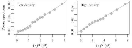
Figure 1: Periodogram power spectrum estimate for the speed time-series of pedestrians at low and high density levels. The power spectrum is roughly proportional to the inverse of square frequency $1/f^{2}$. This is a typical characteristic of Brownian noise.

2.2 Model definition

In the following we therefore introduce a continuous stochastic model to describe one-dimensional pedestrian motion in single-file experiments. We denote the curvilinear position of pedestrian $k$ at time $t$ by $x_{k}(t)$. Pedestrian $k+1$ is the predecessor of $k$. The motion of the pedestrian $k$ is then described by the Langevin equation [40]

$$\left\{\begin{array}[]{lcl}\mbox{d}x_{k}(t)&=&V\big{(}x_{k+1}(t)-x_{k}(t)\big{)}\,\mbox{d}t+\varepsilon_{k}(t)\,\mbox{d}t,\\[1.42262pt] \mbox{d}\varepsilon_{k}(t)&=&-\frac{1}{\beta}\varepsilon_{k}(t)\,\mbox{d}t+\alpha\,\mbox{d}W_{k}(t).\end{array}\right.$$ (1)

where $V:s\mapsto V(s)$ is a differentiable and non-decreasing optimal velocity (OV) function for the convection [8]. The noise $\varepsilon_{k}(t)$ is described by an Ornstein-Uhlenbeck stochastic process [42].

For simplicity, the OV function is chosen as an affine function

$$V(s)=\frac{1}{T}(s-\ell)$$ (2)

in the following, where $T$ is the time gap between the agents and $\ell$ their size. This form is not realistic for very small densities since it is not bounded by some maximal velocity. However, here we are only interested in the congested regime, i.e. intermediate and high densities so that this problem is irrelevant since our systems are one-dimensional with periodic boundary conditions. The quantities $(\alpha,\beta)$ in (1) are parameters related to the noise: $\alpha$ is the volatility and $\beta$ the noise relaxation time. Finally, $W_{k}(t)$ is a Wiener process.

The model can be considered as a special stochastic variant of the Full Velocity Difference model [43]. Writing $\dot{x}_{k}=\mbox{d}x_{k}/\mbox{d}t$, $\ddot{x}_{k}=\mbox{d}^{2}x_{k}/\mbox{d}^{2}t$ and $\mbox{d}W_{k}/\mbox{d}t=\xi_{k}$ as a white noise, one gets from Eq. (1) the second order system

$$\ddot{x}_{k}=\big{[}V(x_{k+1}-x_{k})-\dot{x}_{k}\big{]}/\beta+V^{\prime}(x_{k+1}-x_{k})(\dot{x}_{k+1}-\dot{x}_{k})+\alpha\xi_{k}.$$ (3)

This is a noisy version of the Full Velocity Difference model [43] for which the relaxation time for the speed difference is the derivative of the optimal velocity function.

At this point we want to emphasize a characteristic property of the proposed model. The convection part (first equality in (1)) is of first order, while the noise operates at second order (second equation in (1)). The first order nature of the convection part reflects the assumption that for pedestrian motion inertia effects are less relevant than for vehicular traffic. Instead it is often assumed that pedestrians can stop or accelerate immediately which is naturally described by a first order equation without a mass term.

3 Stability analysis

We now consider one-dimensional motion of $n$ agents on a line of length $L$ with periodic boundary conditions. The dynamics defined in Eq. (1) can be written as a system of equations,

$$\mbox{d}\eta(t)=(A\eta(t)+a)\,\mbox{d}t+b\,\mbox{d}w(t)$$ (4)

with

$$\eta(t) = \operatorname*{\,{}^{\mbox{\tiny T}}\!}\left(x_{1}(t),\varepsilon_{1}(t),\ldots,x_{n}(t),\varepsilon_{n}(t)\right),$$

$$a = -\frac{\ell}{T}\operatorname*{\,{}^{\mbox{\tiny T}}\!}(1,0,\ldots,1,0),$$ (5)

$$b = \alpha\operatorname*{\,{}^{\mbox{\tiny T}}\!}(0,1,\ldots,0,1)$$

and

$$A=\left[\begin{matrix}R&S&\\[-6.82864pt] &\ddots&\\[-6.82864pt] S&&R\end{matrix}\right]\quad\text{with\ \ \ }R=\left[\begin{matrix}-1/T&1\\ 0&-1/\beta\end{matrix}\right],\quad S=\left[\begin{matrix}1/T&0\\ 0&0\end{matrix}\right]\,.$$ (6)

$A$ is a real $2n\times 2n$ matrix, while $\eta(t)$, $a$, $b$ are real $2n$-component vectors. $w(t)$ is $2n$-vector composed of independent Wiener processes. Such a linear stochastic process is Markovian. It has a normal distribution with expectation $m(t)$ and variance/covariance matrix $C(t)$ such that, by using the Fokker-Planck equation (Kolmogorov forward equation)

$$\dot{m}(t)=Am(t)+a\qquad\mbox{and}\qquad\dot{C}(t)=AC(t)+(C(t))\!\operatorname*{\,{}^{\mbox{\tiny T}}\!}A+\mbox{diag}(b)\quad$$ (7)

with $m(0)=\eta_{0}$ and $C(0)=0$. Asymptotically the expectation value $m(t)$ is given by the homogeneous solution for which $x_{k+1}(t)-x_{k}(t)=L/n$ and $\varepsilon_{k}(t)=0$ (for all $k$ and $t$ and by taking $x_{k+1}-x_{k}=x_{1}-x_{n}$ for $k=n$). The matrix $A$ is circulant with blocks of size $2\times 2$. Its eigenvalues are those of $R+S\iota_{\theta}$, with $\iota_{\theta}=e^{i\theta}$ where $\theta=2\pi k/N\in(0,2\pi)$ ($k=0,\ldots,n-1$) is the $n$-th root of unity. The eigenvalues are then the solutions of the characteristic equation

$$\left[\lambda+\frac{1}{T}\big{(}1-e^{i\theta}\big{)}\right]\big{[}\lambda+1/\beta\big{]}=0\,.$$ (8)

The solutions are $\lambda_{1}=-\frac{1}{T}\big{(}1-e^{i\theta}\big{)}$ and $\lambda_{2}=-1/\beta$. They have strictly negative real parts $\mbox{Re}(\lambda_{1})=-\frac{1}{T}(1-\cos(\theta))$ and $\mbox{Re}(\lambda_{2})=-1/\beta$ for any $\theta\in(0,2\pi)$, $T>0$ and $\beta>0$. Therefore the homogeneous solutions are linearly stable for the system (4) for any positive value of the parameters. The least stable configuration is the one with maximal period for which $\theta\rightarrow 0$ (see Fig. 2).

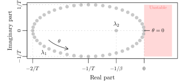
Figure 2: Eigenvalues for the matrix of the linear system for $n=50$. The homogeneous solution is stable when all the eigenvalues have strictly negative real part excepted the one for $\theta=0$, which is null.

Note that the general stability conditions for 2nd order models given for instance in [3, Chap. 15] are

$$a>0,\qquad b+|c|<0,\qquad b^{2}-c^{2}>2a\,,$$ (9)

where $a$, $b$ and $c$ are the partial derivatives of the model according to the distance spacing, the speed of the considered vehicle, and the speed of its predecessor, respectively. For the 2nd order formulation of the model given in Eq. (3) this implies

$$a=\frac{1}{T\beta},\qquad b=-\frac{1}{T}-\frac{1}{\beta},\qquad c=\frac{1}{T}\,.$$ (10)

It is easy to check that all the three conditions in Eq. (9) hold, i.e. the homogeneous solution are deterministically stable, as soon as $T>0$ and $\beta>0$. This confirms the results obtained above.

4 Numerical experiments

We have simulated the system (4) using an explicit Euler-Maruyama numerical scheme with time step $\delta t=0.01$ s. The other parameter have been chosen as $T=1$ s, $\ell=0.3$ m, $\alpha=0.1$ ms^-3/2 and $\beta=5$ s which is close to estimates for pedestrian flow [40]. Corresponding to the experimental situation, the system length is $L=25$ m with periodic boundary conditions.

Simulations have been performed for the model defined by Eq. (4) and, for comparison, the unstable deterministic optimal velocity model with two predecessors in interaction introduced in [44]

$$\dot{x}_{k}=V\big{(}x_{k+1}-x_{k}-T^{r}\big{[}V(x_{k+2}-x_{k+1})-V(x_{k+1}-x_{k})\big{]}\big{)}$$ (11)

Here the optimal velocity function and value is the same as in the stochastic model, i.e. $V(s)=\frac{1}{T}(s-\ell)$ with also $T=1$ s, $\ell=0.3$ m, while the reaction time parameter is set to $T^{r}=0.7$ s in order to describe unstable homogeneous configuration. Starting from a jam initial condition the dynamics of $n=25$, $50$ and $75$ pedestrians has been simulated for both models. Fig. 3 shows typical trajectories for the first two minutes.

Fig. 4 shows the mean autocorrelation functions for the distance spacing for large simulation times $t>t_{S}$, with $t_{S}\,$2$\cdot$10${}^{\text{5}}$ s, where the system can be considered to be in the stationary state. The peaks of the autocorrelations match for both models, indicating identical frequencies of the stop-and-go waves. A wave propagates backwards in the system at speed $c=-\ell/T$ while vehicles travel forward with average speed $v=(L/n-\ell)/T$, where is $T$ the time gap parameter of the optimal velocity function. In agreement with the LWR theory for traffic flow [45, 46], the wave period is $L/(v-c)=nT$.

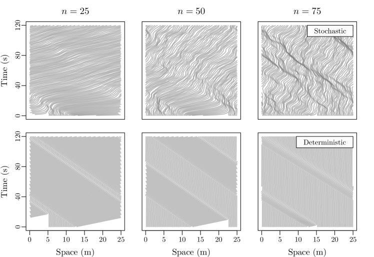
Figure 3: Simulated trajectories for different densities ($n=25,50,75$ pedestrians, $L=25$ m) and jam initial conditions. Top panels: Stochastic model defined by (4). Bottom panels: Unstable deterministic model from [44]. Parameter values are $T=1$ s and $\ell=0.3$ m for the affine optimal velocity of both models, $\alpha=0.1$ ms^-3/2 and $\beta=5$ s for the noise of the stochastic model and $T^{r}=0.7$ s for the reaction time parameter of the deterministic model.

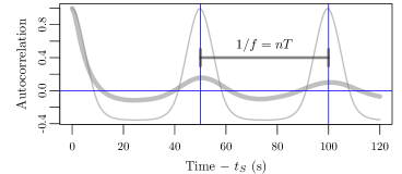
Figure 4: Stationary mean time-correlation function of the distance spacing for the stochastic (thick line) and the deterministic model (thin line). For stop-and-go waves, the same period $1/f=nT$ is observed. The system can be considered stationary after $t_{S}=\,$2$\cdot$10${}^{\text{5}}$ s.

We have also determined the dependence of the results on the noise parameters $\alpha$ and $\beta$. Fig. 5 shows trajectories of $50$ agents for $\alpha=0.05$, $0.1$ and $0.2$ ms^-3/2. The values of $\beta$ are chosen such that the amplitude of the noise $\sigma=\alpha\sqrt{\beta/2}$ is constant, i.e. $\beta=1.25$, $5$ and $20$ s, respectively. For small relaxation times $\beta$, the noise tends to be white and unstable waves emerge locally and disappear (see Fig. 5, left panel). For large $\beta$, on the other hand, the noise autocorrelation is high. In this case stable waves with large amplitude occur (Fig. 5, right panel). Not that the noise parameters influence only the amplitude of the time-correlation function, but not the frequency that only depends on the parameters $n$ and $T$ (see Fig. 6).

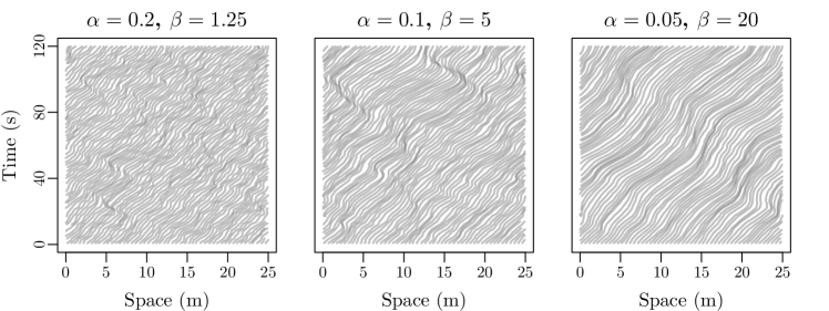
Figure 5: Simulated trajectories of $n=50$ agents for different values of the noise parameters (units: $\alpha$ in ms^-3/2, $\beta$ in s). The initial configuration is homogeneous.

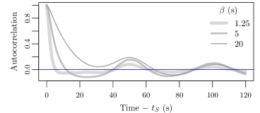
Figure 6: Mean temporal correlation function of the distance spacing in the stationary state of (4) for different values of noise parameter $\beta$. $\alpha$ is chosen such that the noise amplitude is the same in all cases. The noise parameters do not influence the frequency of the waves which only depends on $n$ and $T$.

In Fig. 7 empirical trajectories from experiments with $28$, $45$ and $62$ participants [40] are compared with simulations of the stochastic model. The data show a good agreement. Homogeneous free flow states are observed for $n=28$ agents in both cases, while stop-and-go waves appear in the semi-congested ($n=45$) and congested ($n=62$) states in both data sets.

Figure 7: Empirical (top panels) and simulated (bottom panels) trajectories for different densities. The initial configuration is homogeneous both in the experiments and the simulations.

5 Discussion

We have presented an alternative explanation for the occurrence of stop-and-go phenomena in pedestrian flows. In contrast to previous explanations, the formation of stop-and-go waves here is the consequence of coloured noise in the dynamics of the pedestrian speeds which has been observed in empirical data for single-file motion. This correlated noise can provide perturbations that lead to oscillations in the system, especially when the system is poorly damped. This new mechanism differs that in classical deterministic traffic models with inertia. Here stop-and-go waves occur as a consequence of the instability of the homogeneous configuration. In such a situation s single small perturbation $\varepsilon$ is sufficient to drive the system via a phase transition into a state with periodical dynamics (see Fig. 8, left). In the noise-induced mechanism proposed here the correlated noise can ’kick’ the system out of its stable homogeneous state into a non-homogeneous state in which a damped oscillation is continuously maintained by the perturbations from the noise (see Fig. 8, right).

The two mechanisms differ also in the relevant relaxation processes. In the novel stochastic approach, the relaxation time is related to the noise and is estimated to approximately 5 s [40]. The parameter corresponds to the mean time period of the stochastic deviations from the phenomenological equilibrium state. Such a time can be large, especially for small deviations and large spacings. In contrast, in the classical inertial approaches, the relaxation time is interpreted as the driver/pedestrian reaction time and is estimated to around 0.5 to 1 s. Technically, such a parameter can not exceed the physical time gap between the agents (around 1 to 2 s) without generating unrealistic behaviour (e.g. collisions) and has to be set carefully for these models.

We believe that the new mechanism based on a first order convection equation is specially relevant for pedestrian dynamics. The motion of pedestrians is believed to be much less influenced by inertia effects than the motion of vehicles and is thus much more effect by noise, especially by correlated noises. Due to the limited inertia effects a description based on a first order model is much more natural for pedestrian dynamics. This would also avoid many of the artefacts observed in force-based models (see e.g. [47] and references therein) which are often a consequence of strong inertia effects. In future studies we expect an even better agreement with empirical data when more realistic optimal velocity functions are used in the model. Furthermore, extensions of the model should be carried out to describe the motion of pedestrians in two dimensions, including models for the direction and the definition and meaning of time gap in 2D.

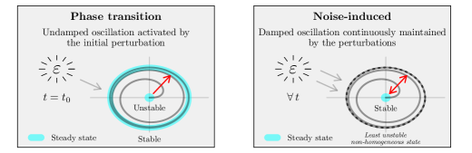
Figure 8: Illustrative scheme for the modelling of stop-and-go dynamics with phase transition in the periodic solution (left panel) and the noise-induced oscillating behaviour (right panel).

Conflict of interest

The authors do not have any conflict of interest with other entities or researchers.

References

- [1] D. Chowdhury, L. Santen, and A. Schadschneider. Statistical physics of vehicular traffic and some related systems. Phys. Rep., 329:199–329, 2000.
- [2] B.S. Kerner. The Physics of Traffic. Springer-Verlag, 2004.
- [3] M. Treiber and A. Kesting. Traffic Flow Dynamics. Springer, Berlin, 2013.
- [4] A. Schadschneider, M. Chraibi, A. Seyfried, A. Tordeux, and J. Zhan. TBA, chapter Pedestrian Dynamics – From Empirical Results to Modeling. Birkhäuser-Springer, 2018.
- [5] M. Chraibi, A. Tordeux, A. Schadschneider, and A. Seyfried. Encyclopedia of Complexity and Systems Science, chapter Pedestrian and Evacuation Dynamics – Modelling. Springer, 2018.
- [6] J. Zhang, W. Mehner, S. Holl, M. Boltes, E. Andresen, A. Schadschneider, and A. Seyfried. Universal flow-density relation of single-file bicycle, pedestrian and car motion. Phys. Lett. A, 378:3274–3277, 2014.
- [7] Y. Sugiyama, M. Fukui, M. Kikushi, K. Hasebe, A. Nakayama, K. Nishinari, and S. Tadaki. Traffic jams without bottlenecks. Experimental evidence for the physical mechanism of the formation of a jam. New J. Phys., 10:033001, 2008.
- [8] M. Bando, K. Hasebe, A. Nakayama, A. Shibata, and Y. Sugiyama. Dynamical model of traffic congestion and numerical simulation. Phys. Rev. E, 51:1035–1042, 1995.
- [9] D. Helbing and M. Treiber. Gas-kinetic-based traffic model explaining observed hysteretic phase transition. Phys. Rev. Lett., 81:3042–3045, 1998.
- [10] R.M. Colombo. Hyperbolic phase transitions in traffic flow. SIAM J. Appl. Math., 63:708–721, 2003.
- [11] M. Muramatsu and T. Nagatani. Soliton and kink jams in traffic flow with open boundaries. Phys. Rev. E, 60:180–187, 1999.
- [12] E Tomer, L. Safonov, and S. Havlin. Presence of many stable nonhomogeneous states in an inertial car-following model. Phys. Rev. Lett., 84:382–385, 2000.
- [13] E. Ben-Jacob, O. Schochet, A. Tenenbaum, I. Cohen, A. Czirok, and T. Vicsek. Generic modelling of cooperative growth patterns in bacterial colonies. Nature, 368:46–49, 1994.
- [14] T. Vicsek, A. Czirók, E. Ben-Jacob, I. Cohen, and O. Shochet. Novel type of phase transition in a system of self-driven particles. Phys. Rev. Lett., 75:1226–1229, 1995.
- [15] H.J. Bussemaker, A. Deutsch, and E. Geigant. Mean-field analysis of a dynamical phase transition in a cellular automaton model for collective motion. Phys. Rev. Lett., 78:5018–5021, 1997.
- [16] J. Buhl, D. J. T. Sumpter, I. D. Couzin, J. J. Hale, E. Despland, E. R. Miller, and S. J. Simpson. From disorder to order in marching locusts. Science, 312:1402–1406, 2006.
- [17] G Hermann and J Touboul. Heterogeneous connections induce oscillations in large-scale networks. Phys. Rev. Lett., 109:018702, 2012.
- [18] B. S. Kerner and H. Rehborn. Experimental properties of phase transitions in traffic flow. Phys. Rev. Lett., 79:4030–4033, 1997.
- [19] M. Treiber, A. Kesting, and D. Helbing. Three-phase traffic theory and two-phase models with a fundamental diagram in the light of empirical stylized facts. Transport. Res. B: Meth., 44:983–1000, 2010.
- [20] A. Seyfried, A. Portz, and A. Schadschneider. Phase coexistence in congested states of pedestrian dynamics. Lect. Notes Comp. Sci., 6350:496–505, 2010.
- [21] A. Portz and A. Seyfried. Modeling stop-and-go waves in pedestrian dynamics. Lecture Notes in Computer Science, 6068:561–568, 2010.
- [22] M. Moussaïd, D. Helbing, and G. Theraulaz. How simple rules determine pedestrian behavior and crowd disasters. Proc. Nat. Acad. Sci., 108:6884–6888, 2011.
- [23] H. Kuang, Y. Fan, X. Li, and L. Kong. Asymmetric effect and stop-and-go waves on single-file pedestrian dynamics. Procedia Eng., 31:1060 – 1065, 2012.
- [24] S. Lemercier, A. Jelic, R. Kulpa, J. Hua, J. Fehrenbach, P. Degond, C. Appert-Rolland, S. Donikian, and J. Pettré. Realistic following behaviors for crowd simulation. Comput. Graph. Forum, 31:489–498, 2012.
- [25] R. Barlovic, L. Santen, A. Schadschneider, and M. Schreckenberg. Metastable states in cellular automata for traffic flow. EPJB, 5:793–800, 1998.
- [26] W. Knospe, L. Santen, A. Schadschneider, and M. Schreckenberg. Towards a realistic microscopic description of highway traffic. J. Phys. A, 33:L477, 2000.
- [27] P. Hänggi and P. Jung. Colored Noise in Dynamical Systems, chapter 4, pages 239–326. John Wiley & Sons, Inc., 2007.
- [28] D. Helbing, I.J. Farkas, and T. Vicsek. Freezing by heating in a driven mesoscopic system. Phys. Rev. Lett., 84:1240–1243, 2000.
- [29] L. Arnold, W. Horsthemke, and R. Lefever. White and coloured external noise and transition phenomena in nonlinear systems. Z. Phys. B Con. Mat., 29:367–373, 1978.
- [30] F. Castro, A. D. Sánchez, and H. S. Wio. Reentrance phenomena in noise induced transitions. Phys. Rev. Lett., 75:1691–1694, 1995.
- [31] D.L. Gilden, T. Thornton, and M.W. Mallon. noise in human cognition. Science, 267:1837–1839, 1995.
- [32] A. Zgonnikov, I. Lubashevsky, S. Kanemoto, T. Miyazawa, and T. Suzuki. To react or not to react? Intrinsic stochasticity of human control in virtual stick balancing. J. R. Soc. Interface, 11, 2014.
- [33] R.W. Williams and K. Herrup. The control of neuron number. Annu. Rev. Neurosci., 11:423–453, 1988.
- [34] D. Helbing and P. Molnár. Social force model for pedestrian dynamics. Phys. Rev. E, 51:4282–4286, 1995.
- [35] M. Takayasu and H. Takayasu. 1/f noise in a traffic model. Fractals, 01:860–866, 1993.
- [36] P. Wagner. How human drivers control their vehicle. EPJ B, 52:427–431, 2006.
- [37] M. Treiber, A. Kesting, and D. Helbing. Delays, inaccuracies and anticipation in microscopic traffic models. Phys. A, 360:71–88, 2006.
- [38] S.H. Hamdar, H.S. Mahmassani, and M. Treiber. From behavioral psychology to acceleration modeling: Calibration, validation, and exploration of drivers’ cognitive and safety parameters in a risk-taking environment. Transp. Res. B-Meth., 78:32–53, 2015.
- [39] Forschungszentrum Jülich ped.fz-juelich.de/database.
- [40] A. Tordeux and A. Schadschneider. White and relaxed noises in optimal velocity models for pedestrian flow with stop-and-go waves. J. Phys. A, 49:185101, 2016.
- [41] G. Lindgren, H. Rootzen, and M. Sandsten. Stationary Stochastic Processes for Scientists and Engineers. Taylor & Francis, 2013.
- [42] N.G. van Kampen. Stochastic Processes in Physics and Chemistry. Elsevier, 2007.
- [43] R. Jiang, Q. Wu, and Z. Zhu. Full velocity difference model for a car-following theory. Phys. Rev. E, 64:017101, 2001.
- [44] A. Tordeux and A. Seyfried. Collision-free nonuniform dynamics within continuous optimal velocity models. Phys. Rev. E, 90:042812, 2014.
- [45] P. I. Richards. Shock waves on a highway. Op. Res., 4(1):42–51, 1956.
- [46] M. H. Lighthill and G. B. Whitham. On kinematic waves II: a theory of traffic flow on long, crowded roads. In Proceedings of the Royal Society of London series A, volume 229, pages 317–345, 1955.
- [47] M. Chraibi, T. Ezaki, A. Tordeux, K. Nishinari, A. Schadschneider, and A. Seyfried. Jamming transitions in force-based models for pedestrian dynamics. Phys. Rev. E, 92:042809, 2015.