Introduction to Solving Quant Finance Problems with Time-Stepped FBSDE and Deep Learning

Abstract

In this introductory paper, we discuss how quantitative finance problems under some common risk factor dynamics for some common instruments and approaches can be formulated as time-continuous or time-discrete forward-backward stochastic differential equations (FBSDE) final-value or control problems, how these final value problems can be turned into control problems, how time-continuous problems can be turned into time-discrete problems, and how the forward and backward stochastic differential equations (SDE) can be time-stepped. We obtain both forward and backward time-stepped time-discrete stochastic control problems (where forward and backward indicate in which direction the $Y$ SDE is time-stepped) that we will solve with optimization approaches using deep neural networks for the controls and stochastic gradient and other deep learning methods for the actual optimization/learning. We close with examples for the forward and backward methods for an European option pricing problem. Several methods and approaches are new.

1 Introduction

This paper is structured as follows: in section 2, we quickly discuss the general risk factor dynamics used. In section 3, we describe the prototypical instruments and instrument features treated: Europeans, Barriers, and Bermudans/Exercise opportunities. Section 4 states what we are interested in computing. Section 5 shows how one can obtain (continuous time) FBSDE formulations and FBSDE final value problems from a variety of sources and approaches. Section 6 shows how one can obtain (continuous time) FBSDE stochastic control formulations. Section 7 shows how one can obtain (discrete time) FBSDE stochastic control formulations for the introduced financial instruments. Section 8 describes how these discrete time FBSDE stochastic control problems can be solved by deep neural networks and deep learning. Section 9 presents the application of the forward and the backward methods to European option pricing problem for a one-dimensional example which allows good visualization and understanding. Section 10 concludes.

2 Risk Factor Dynamics

The vector of risk factors $X_{t}$ under consideration is assumed to follow the SDE:

$$dX_{t}=\mu\left(t,X_{t}\right)dt+\sigma_{N}\left(t,X_{t}\right)dW_{t}$$ (1)

The operator connected to the risk factor dynamics is:

$${\cal L}_{t}u\left(t,x\right):=\frac{1}{2}\text{Tr}\left(\sigma_{N}\sigma_{N}^{T}\left(t,x\right)\left(\text{Hess}_{x}u\right)\left(t,x\right)\right)+\mu\left(t,x\right)\nabla u\left(t,x\right)$$ (2)

where $\text{Hess}_{x}u$ is the Hessian matrix.

For the case of constant volatility, constant interest rate, risk neutral Black-Scholes on a single underlier, $\mu(t,X_{t})=rX_{t}$ and $\sigma_{N}(t,X_{t})=\sigma_{BS}X_{t}$, and ${\cal L}_{t}u=\frac{1}{2}\sigma_{BS}^{2}X^{2}u_{xx}+rXu_{x}$.

Most often, we will assume that the dynamics is given under the risk neutral measure where $\mu(t,X_{t})=r(t)X_{t}$ for tradeable components of $X_{t}$ or under numeraire measures in which $\mu(t,X_{t})$ is zero and the components of $X$ are measured in units of numeraire. We also typically assume (in particular for the trading strategy set-up) that the volatility is given in log-normal terms $\sigma_{N}(t,X_{t})=\sigma_{LN}(t,X_{t})X_{t}$ (with multiplication understood elementwise).

Typically one assumes at least one locally riskless basic security (money market instrument or bond) with an equation like the following:

$$dB=r\left(t\right)B\left(t\right)\text{dt}$$

or alternatively a risk-free zero-coupon bond or similar instrument (the expression and/or SDE for such bonds depends on the chosen model).

3 Instruments covered

In this introduction, we will only cover relatively simple instruments with a few key features. Many instruments with more complicated features can be treated very similarly with the same approaches and ideas.

3.1 Europeans

At a given payment time $T^{P}$, called typically instrument maturity, a European option instrument pays $g(X(T^{P}))$. $X$ is the vector of the risk factors. (It might well be that the final payoff does not depend on any risk factor or on only one.) For a stock-option, $X$ would be the stock price. For a short-rate model, the risk factor could be the short rate $r(t)$, or if the formulation requires a tradeable financial instrument, it could a bank account $B(t)$ or zero coupon bond $P(t)$ under that short rate model, and the quantity that is used to determine the payment amount could be a forward rate (which can also be written in terms of a ratio of two bond prices) $L$.

The two most common basic payoffs are call and put options on some single underlier $X_{i}(T^{P})$ with strike $K$, paying $\mathsf{max}(X_{i}(T^{P})-K,0)$ and $\mathsf{max}(K-X_{i}(T^{P}),0)$ respectively.

3.2 Simple Barriers

Barrier options are options that will pay only if some barrier level or region is touched (knocked-in) or not touched (knock-out), or change final payout upon touching a barrier. The simplest barrier options are those with a single barrier at some constant level which is active for the entire life of the instrument.

Once again, two standard examples: A standard up-and-out barrier call option with upper barrier $B$ will pay the final call payoff unless the underlier $S$ of the option was observed at a level $S\geq B$ during the life of the option and otherwise will pay nothing. A standard up-and-in barrier call option with upper barrier $B$ will pay the final call payoff only if the underlier $S$ of the option was observed at a level $S\geq B$ during the life of the option and otherwise will pay nothing.

In terms of simulation or simulation-like approaches, one follows the risk factor simulation until maturity or barrier breach (whatever comes first) and then uses the final value or the value of the knocked-in instrument on/in the barrier (or zero, if there is no knock-in).

3.2.1 Special case: Treatment as European

We will explain the case of an upper barrier at a constant level $B$: Call $\textrm{PBreach}(X_{T};X_{0})$ the probability that the barrier was breached given initial and final value $P(X_{t}\geq B|0<t<T,X_{0},X_{T}))$ and call the payout when triggered $g_{B}(X_{T})$ and when not triggered $g_{NB}(X_{T})$. If the final value of $X$ is not beyond the barrier, the final value of the instrument is either $g_{B}(X_{T})$ with probability $\textrm{PBreach}(X_{T};X_{0})$ or $g_{NB}(X_{T})$ with probability $(1-\textrm{PBreach}(X_{T};X_{0}))$; if it is beyond the barrier, it will be $g_{B}(X_{T})$.

For purposes of valuation as of time 0, the value of the barrier option will agree with the value of an European option with the final value

$$g(X_{T})=\left\{\begin{array}[]{lr}g_{NB}(X_{T})(1-\textrm{PBreach}(X_{T};X_{0}))+g_{B}(X_{T})\textrm{PBreach}(X_{T};X_{0})&\textrm{if not }X_{T}\geq B\\ g_{B}(X_{T})&\textrm{if }X_{T}\geq B\\ \end{array}\right.$$ (3)

This can be solved just like any other European option pricing problem. Notice that this will only give the correct price if the barrier has not been breached at valuation time.

Yu, Xing, and Sudjianto [YXS19] have used a variant of this approach to solve some barrier options with the standard European deepBSDE approach.

3.3 Exercise opportunity

Assume that at some time $t_{E}<T$, the holder of the instrument has a choice to either exercise into an immediate payment worth $g_{E}(X_{t_{E}})$ (or into an instrument expected to be worth $g_{E}(X_{t_{E}})$) or continuing to hold on to the instrument with the given final payment $g(X(T^{P}))$.

Exercise opportunities are often handled by either computing an expected holding value/continuation value $\mathsf{hv}(X_{t_{E}})$ and exercising when the exercise value is larger than the holding value ($g_{E}(X_{t_{E}})>\mathsf{hv}(X_{t_{E}})$) or by defining an exercise strategy $\mathsf{es}(X_{t_{E}})$ that is only true/one when the instrument should be exercised and false/zero otherwise. Given some holding value function or exercise strategy function, an exercise opportunity can be directly simulated and pricing happens like the barrier case (where different actions are taken depending on whether the barrier was hit or not).

Proceeding from the last exercise opportunity to the first, the case of finitely many exercise opportunities can be reduced to the case of a single exercise opportunity. Exercise time intervals can be approximated by appropriately frequent discrete exercise times.

4 Analytics to be computed

At a minimum, we want to compute the value at initial time with given fixed risk factor values. (This corresponds to the dynamics being started at $X_{0}=x_{0}$ with $x_{0}$ being those fixed risk factor values.) In many situations, we would like to compute the value at initial time with risk factor values within a certain range around some given fixed values (for sensitivities and other purposes). This can be achieved by modeling $X_{0}$ as a random variable with the appropriate domain, for instance.

The methods that we will present will compute simulated instrument values along simulated paths. Forward methods will give us simulated instrument values conditional on the shared past. Backward methods will give simulated instrument values that take future values of the risk factors and of the instrument value into account. To convert to instrument values conditional on the shared past, an adapted projection or approximation needs to be computed from the simulation results of the backward methods.

In general, it would be useful to determine the instrument value at certain intermediate times over a certain range of risk factors. This can be achieved for instance by starting the computation at a future time $t_{0}$ with random $X_{t_{0}}$ with the appropriate domain of interest, but potentially also with other approaches. For instance, this can be used to compute holding values for exercise opportunities.

5 Obtaining time-continuous FBSDE final value problems for Quantitative Finance problems

A time continuous FBSDE problem has the following form:

The forward SDE (FSDE) for the dynamics:

$$dX_{t}=\mu\left(t,X_{t}\right)dt+\sigma_{N}\left(t,X_{t}\right)dW_{t}$$ (4)

and the backward SDE (BSDE) for the value in terms of volatility scaled values $Z_{t}$:

$$-dY_{t}=f_{Z}\left(t,X_{t},Y_{t},Z_{t}\right)dt\ -Z_{t}^{T}dW_{t}$$ (5)

or in terms of values $\Pi_{t}$:

$$-dY_{t}=f\left(t,X_{t},Y_{t},\Pi_{t}\right)dt\ -\Pi_{t}^{T}\sigma_{LN}\left(t,X_{t}\right)dW_{t}$$ (6)

A final value problem adds the final value condition for $Y$

$$Y_{T}=g(X_{T})$$ (7)

For fixed initial risk factor values, the forward dynamics is completed by $X_{0}=x_{0}$. For the case of random $X_{0}$, $X_{0}$ will be a random variable.

For short introductions into FBSDE in finance and otherwise, see, for instance, El Karoui, Peng, and Quenez [EKPQ97] and Perkowski [Per10].

5.1 Linear PDE

A linear partial differential equation (PDE) of the form:

$$u_{t}\left(t,x\right)+{\cal L}_{t}u\left(t,x\right)-V\left(t,x\right)u\left(t,x\right)+h\left(t,x\right)=0$$ (8)

can be written as a FBSDE with the generator function $f$ as follows:

$$f(t,X,Y,\Pi)=-V(t,X)Y+h(t,X)$$ (9)

as a special case of a nonlinear Feynman-Kac theorem (which will be presented below).

5.2 Risk Neutral Expectations

Assume the solution is characterized by

$$u\left(t,x\right)={B\left(t\right)E}\left(\frac{g\left(X_{T}\right)}{B(T)}\middle|X_{t}=x\right)$$ (10)

with

$$\frac{B(t)}{B(T)}=\exp\left(-\int_{t}^{T}r\left(s\right)ds\right)$$ (11)

Then the solution $u$ can be written as $u(t,X)=Y_{t}$ where $X_{t}=X$ and $Y$ solves a FBSDE with generator function $f$ as follows:

$$f(t,X,Y,\Pi)=-r(t)Y$$ (12)

5.3 Expectations under Numeraire Measures

Assume the solution is characterized by

$$\frac{u\left(t,x\right)}{N(t)}=E\left(\frac{g\left(X_{T}\right)}{N(T)}\middle|X_{t}=x\right)$$ (13)

with some deterministic or stochastic dynamics for the numeraire $N(t)$, where $E$ is in the measure corresponding to the numeraire $N(t)$. Under that measure, the relative value of the instrument as measured in units of numeraire is a martingale. Therefore, the generator function $f$ will be zero.

The solution $u(t,X)$ will be given as $u(t,X)=N(t)Y_{t}$ where $X_{t}=X$ and $Y$ solves a FBSDE with a zero generator function.

5.4 Nonlinear PDE

One of the nonlinear Feynman-Kac theorems states (El Karoui, Peng, and Quenez [EKPQ97] and Perkowski [Per10]) that under appropriate assumptions, the solution of

$$u_{t}\left(t,x\right)+{\cal L}_{t}u\left(t,x\right)+f\left(t,x,u\left(t,x\right),\nabla u\left(t,x\right)\right)=0$$ (14)

is given as the $Y$ solution $Y_{t}$ of a BSDE

$$-dY_{t}=f\left(t,X_{t},Y_{t},\Pi_{t}\right)dt\ -\Pi_{t}^{T}\sigma\left(t,X_{t}\right)dW_{t}$$ (15)

The $\Pi$ solution of the BSDE will be $\Pi_{t}=\nabla_{X}u(t,X_{t})$.

5.5 Self-Financing Conditions

Instead of deriving the BSDE from other formulations, one can directly derive BSDE from self-financing conditions if one assumes that the components of $X$ are basic underlying securities (or, at least, that there are enough instruments that depend on such components of $X$ and that hedge ratios for such instruments can be computed from the sensitivities to the components). The corresponding component of $\Pi_{t}$ (the trading strategy portfolio) describes how much of the portfolio value is invested in that component of $X_{t}$. The remainder of $Y_{t}$, $\pi_{0}(t)=Y_{t}-\Pi\cdot 1$, is assumed to be invested in cash.

Under the assumptions of risk neutral pricing (among them, that both positive cash balances (which can be lent out) and negative cash balances (which corresponds to amounts borrowed) attract the same interest rate $r(t)$ - deterministic or stochastic), one obtains a BSDE for the portfolio value $Y_{t}$ with generator function $f$ as follows:

$$f(t,X,Y,\Pi)=-r(t)Y$$ (16)

Assuming that positive cash amounts attract an interest rate $r^{l}(t)$ and negative cash amounts attract an interest rate $r^{b}(t)>r^{l}(t)$ and that the components of $X_{t}$ have a drift of $r^{l}(t)X_{t}$ (this setting is called “differential rates”), then the $f$ generator function in the BSDE is as follows:

$$f(t,X(T),Y(t),\Pi_{t})=-r^{l}(t)Y(t)+(r^{b}(t)-r^{l}(t))\left(\sum_{i=1}^{n}\pi_{i}(t)-Y(t)\right)^{+}$$ (17)

Transaction cost can be included if the generator $f$ is allowed to depend on the time-derivative $\dot{\pi}_{i}(t)$ of $\pi_{i}(t)$ as well, with $G(x)=\lambda|x|^{q}/q$ with $q\in(1,2]$ and additional terms $-G(\dot{\pi}_{i}(t))$ for all the components with transaction costs added to the $f$ generator function in the BSDE, as in Gonon, Muhle-Karbe, and Shi [GMKS19]. (Alternatively, the transaction costs can be included in the running cost in the stochastic control problem introduced below.) However, it is easier to handle transaction costs in the time-discrete setting.

6 Obtaining time-continuous FBSDE stochastic control problems

A general stochastic control problem based on some underlying stochastic evolving factors $\tilde{X}$ asks for a control function $c_{t}$ that minimizes or maximizes the functional

$$\tilde{J}(c)=E\left(\int_{0}^{T}\tilde{\mathsf{rc}}(s,\tilde{X}_{s},c_{s})ds+\tilde{\mathsf{fc}}(\tilde{X}_{T})\right)$$ (18)

where $\tilde{X}$ follows:

$$d\tilde{X}_{t}=\tilde{\mu}\left(t,\tilde{X}_{t};c_{t}\right)dt+\tilde{\sigma}\left(t,\tilde{X}_{t};c_{t}\right)dW_{t}$$ (19)

and $\mathsf{rc}$ and $\mathsf{fc}$ are running cost and final cost functions, respectively. In the standard exposition, $\tilde{X}_{0}$ is typically given as fixed value, but part of it could be part of the control and/or a function of some other components of $\tilde{X}$ where the particular function is determined as part of the solution of the control problem.

One can also derive a BSDE that characterizes the optimal control for this stochastic control problem. However, here $\tilde{X}$ will be the concatenation of the $X_{t}$ vector and the $Y_{t}$ value and thus the underlying stochastic evolving factors will obey

$$dX_{t}=\mu\left(t,X_{t}\right)dt+\sigma\left(t,X_{t}\right)dW_{t}$$ (20)

$$dY_{t}=-f\left(t,X_{t},Y_{t},\Pi_{t}\right)dt\ +\Pi_{t}^{T}\sigma\left(t,X_{t}\right)dW_{t}$$ (21)

where $\Pi_{t}$ plays the role of a control and the functional to be minimized or maximized is

$$J^{F}(\Pi_{t},\Pi^{\mathsf{final}},\ldots)=E\left(\int_{0}^{T}{\mathsf{rc}}(s,{X}_{s},Y_{s},\Pi_{s})ds+{\mathsf{fc}}({X}_{T},Y_{T},\Pi^{\mathsf{final}})\right)$$ (22)

Any forward FBSDE stochastic control problem of that form occuring in the literature or in applications can be handled in our approach.

For a very short introduction into stochastic control problems, see Perkowski [Per10].

6.1 From Final Value problems - Forward Approach

If the $Y_{t}$ BSDE is treated in a forward manner, the initial value of $Y$, $Y_{0}$ is part of the control (if $X_{0}$ is a fixed value), while if $X_{0}$ is random, $Y_{0}=Y^{\mathsf{init}}(X_{0}))$ is a function to be determined as part of the stochastic control problem. Transaction costs and similar could be treated as part of the BSDE or as part of the running cost. The final cost will be some (risk) measure on how well the final value is replicated, for instance the $L_{2}$ distance

$$\mathsf{fc}(X_{T},Y_{T})=||Y_{T}-g(X_{T})||^{2}$$ (23)

but other appropriate risk measures are possible also.

The forward approach for fixed $X_{0}$ in the time-discrete case (together with approximating the control with deep neural networks (DNN) and solving the control problem with deep learning (DL)) was introduced and used in applications by E, Han, and Jentzen [EHJ17] and called “deepBSDE” method, a generic name that we will also use.

To the best of our knowledge, Han, Jentzen, and E [HJE18] mention the forward approach for random $X_{0}$ as a possibility on page 8509 but we are not aware of any implementation of this method besides our own.

6.2 From Final Value problems - Backward Approach

Assume that there would be a way to treat the $Y_{t}$ BSDE backward in the time-continuous setting, then one could start with $Y_{T}=g(X_{T})$ and evolve $Y_{t}$ backward until one reaches time 0 or another chosen initial time $t_{0}$.

Under those circumstances, the functional to be minimized or maximized would be

$$J^{B}(\Pi_{t},\Pi^{\mathsf{initial}},\ldots)=E\left(\int_{0}^{T}{\mathsf{rc}}(s,{X}_{s},Y_{s},\Pi_{s})ds+{\mathsf{ic}}({X}_{0},Y_{0},\Pi^{\mathsf{initial}})\right)$$ (24)

If there is a unique solution $Y_{t}$ to the final value problem, that solution should be found as minimizer of a functional where the running cost is zero and the initial cost is given as the variance of $Y_{0}$ (or any other good measure of range or size of domain of $Y_{0}$) if $X_{0}$ is fixed or the $L_{2}$ distance of the $Y_{0}$ from a to-be-determined function $Y^{\mathsf{init}}(X_{0})$ if $X_{0}$ is random. Alternatively, the initial cost could be combination of a variance/range measure and risk measure or one could solve a multi-objective problem with both of those measures as separate objectives.

The backward method for fixed $X_{0}$ in the time-discrete case (together with approximating the control with DNN and solving the control problem with deep learning), to the best of our knowledge, was introduced and used first in Wang et al [WCS⁺18]. The backward method for random $X_{0}$ is new.

7 Obtaining time-discrete FBSDE stochastic control problems

7.1 Time-discretizing time-continuous FBSDE

Applying a simple Euler-Maruyama discretization for both $X_{t}$ and $Y_{t}$, we obtain

$$X_{t_{i+1}}=X_{t_{i}}+\mu(t_{i},X_{t_{i}})\Delta t_{i}+\sigma^{T}(t_{i},X_{t_{i}})\Delta W^{i}$$ (25)

$$Y_{t_{i+1}}=Y_{t_{i}}-f\left(t_{i},X_{t_{i}},Y_{t_{i}},\Pi_{t_{i}}\right)\Delta t_{i}+\Pi^{T}_{t_{i}}\sigma^{T}(t_{i},X_{t_{i}})\Delta W^{i}$$ (26)

This can be used to time-step both $X_{t}$ and $Y_{t}$ forward.

To time-step $Y_{t}$ backward, one needs to solve

$$Y_{t_{i}}-f\left({t_{i}},X_{t_{i}},Y_{t_{i}},\Pi_{t_{i}}\right)\Delta{t_{i}}=Y_{t_{i+1}}-\Pi^{T}_{t_{i}}\sigma^{T}(t_{i},X_{t_{i}})\Delta W^{i}$$ (27)

for $Y_{t_{i}}$ (assuming $\Pi_{t_{i}}$ is given or otherwise determined, such as by control or optimization).

Set $F^{B}$ as the function that satisfies

$$F^{B}(t,\Delta t,X,\Pi,R)-f(t,X,F^{B}(t,\Delta t,X,\Pi,R),\Pi)\Delta t=R$$ (28)

then the exact backward step can be expressed as

$$Y_{t_{i}}=F^{B}(t_{i},\Delta t_{i},X_{t_{i}},\Pi_{t_{i}},Y_{t_{i+1}}-\Pi^{T}_{t_{i}}\sigma^{T}(t_{i},X_{t_{i}})\Delta W^{i})$$ (29)

Instead of an exact solution, one can use Taylor expansion as in Liang, Xu, and Li [LXL19].

The functional will be replaced by an appropriate time-discretized version such as

$$J^{F}(\Pi_{t},\Pi^{\mathsf{final}},\ldots)=E\left(\sum_{0}^{N-1}{\mathsf{rc}}(t_{i},{X}_{t_{i}},Y_{t_{i}},\Pi_{t_{i}})\delta t_{i}+{\mathsf{fc}}({X}_{N},Y_{N},\Pi^{\mathsf{final}})\right)$$ (30)

and

$$J^{B}(\Pi_{t},\Pi^{\mathsf{initial}},\ldots)=E\left(\sum_{0}^{N-1}{\mathsf{rc}}(t_{i},{X}_{t_{i}},Y_{t_{i}},\Pi_{t_{i}})\Delta t_{i}+{\mathsf{ic}}({X}_{0},Y_{0},\Pi^{\mathsf{initial}})\right)$$ (31)

or similar.

7.2 Self-financing conditions

Similarly to the derivation of the self-financing condition for the time-continuous case, assuming a trading strategy vector $\Pi_{t_{i}}$ in force during the time step from $t_{i}$ to $t_{i+1}$, one obtains the part of the time-discrete BSDE for the portfolio value $Y$ as follows

$$\mathsf{driftterm}(t_{i},\Delta t_{i},Y_{t_{i}},\Pi_{t_{i}})+\Pi^{T}_{t_{i}}\sigma_{LN}(t_{i},X_{t_{i}})\Delta W^{i}$$ (32)

where the drift term in the risk neutral case is

$$\mathsf{driftterm}(t_{i},\Delta t_{i},Y_{t_{i}},\Pi_{t_{i}}):=(1+r(t)\Delta t_{i})Y_{t_{i}}$$ (33)

and in the differential rate case is (recall $\pi_{0}(t)=Y_{t}-\Pi\cdot 1$, common growth rate under pricing measure for underliers is $r(t)$)

$$\mathsf{driftterm}(t_{i},\Delta t_{i},Y_{t_{i}},\Pi_{t_{i}}):=Y_{t_{i}}+\Delta t_{i}\left(r(t)\sum_{i=1}^{N}\pi_{i}(t_{i})+\left\{\begin{array}[]{lc}r^{l}(t)\pi_{0}(t_{i})&\textrm{if }\pi_{0}(t_{i})\geq 0\\ r^{b}(t)\pi_{0}(t_{i})&\textrm{else }\\ \end{array}\right.\right)$$ (34)

Dividends or fees for the underlying securities would contribute appropriate terms.

So far we have not found time-discrete FBSDE with transaction costs handled by deepBSDE methods.

Transaction costs can be introduced in the following fashion: Value based transaction costs incurred in the reallocation from $\Pi_{t_{i}}$ to $\Pi_{t_{i+1}}$ contribute terms of the form (where $j$ indicates the component/underlying security that incurs these transaction costs)

$$-\sum_{j=1}^{n}\lambda_{j}\left|\pi_{j}(t_{i+1})-\pi_{j}(t_{i})\right|^{q_{j}}$$ (35)

Per share based transaction costs contribute terms of the form

$$-\sum_{j=1}^{n}\lambda_{j}\left|\frac{\pi_{j}(t_{i+1})}{X_{j}(t_{i+1})}-\frac{\pi_{j}(t_{i})}{X_{j}(t_{i})}\right|^{q_{j}}$$ (36)

A fixed commission that is only charged when there is trading contributes terms of the form (with $1_{x}$ the indicator function):

$$-\sum_{j=1}^{n}\lambda_{j}1_{\pi_{j}(t_{i+1})\neq\pi_{j}(t_{i})}$$ (37)

Whatever the exact form is, the total $Y$ drift term can be written as a function $f_{\Delta t}$ as follows in the time-discrete BSDE for $Y_{i}$:

$$Y_{t_{i+1}}=Y_{t_{i}}-f_{\Delta t}\left(t_{i},\Delta t_{i},X_{t_{i}},X_{t_{i+1}},Y_{t_{i}},Y_{t_{i+1}},\Pi_{t_{i}},\Pi_{t_{i+1}}\right)+\Pi^{T}_{t_{i}}\sigma^{T}(t_{i},X_{t_{i}})\Delta W^{i}$$ (38)

Exact or approximate backward steps can be derived as in the previous subsection.

7.3 Forward time-stepping methods

In these methods, both the risk factors $X_{t_{i}}$ and the portfolio value $Y_{t_{i}}$ are time-stepped forwards.

7.3.1 Europeans

Here, in the functional, there is typically no running cost, and the only term is the $L_{2}$ distance or similar measure on the replication of the final values.

After time-stepping the $Y_{t_{i}}$ forward, the functional given by the final cost term is evaluated and gives the objective/loss function.

Even if the functional would include running costs, one would carry along the running cost together with the $X_{t_{i}}$ and $Y_{t_{i}}$ as, say $J_{t_{i}}$.

7.3.2 Barriers

We will discuss only the case of knock-out barriers with immediate rebate on hitting the barrier. Other barrier option types can be treated similarly.

The evolution of the $X_{t_{i}}$ is monitored and a barrier indicator $\mathsf{Barrier}_{t_{i}}$ is introduced that turns from 0 to 1 when the evolution of the $X_{t_{i}}$ breaches the barrier and otherwise remains constant (in particular it stays at 1 even if $X$ should no longer breach the barrier at a later time). We introduce additional state variables $t^{B}_{t_{j}}$, $X^{B}_{t_{j}}$, and $Y^{B}_{t_{j}}$ that record the time $t_{i}$, the $X_{t_{i}}$, and the $Y_{t_{i}}$ at barrier breach or maturity (whatever comes first) at a time $t_{j}$ at or after the breach/maturity. Depending on the value of $t^{B}_{t_{N}}$ (maturity or not), the final cost is the $L_{2}$ norm of the difference (or other risk measure) between $Y^{B}_{t_{N}}$ and the appropriate payoff $g(X_{t_{N}})$ or $g_{b}(t^{B}_{t_{N}},X^{B}_{t_{N}})$.

This is a new method. We are currently implementing this method with promising results and expect to publish details of the method and results soon.

7.3.3 Exercise Opportunities

First, one determines the exercise strategy or the holding value, for instance by starting forward or backward method with random initial risk factor values at the potential exercise time.

Given $\mathsf{hv}(X_{t_{E}})$, at time $t_{E}$, we will check $g_{E}(X_{t_{E}})>\mathsf{hv}(X_{t_{E}})$. If that is true, $t_{E}$ will be marked as exercise time $t^{E}$, $X_{t_{E}}$ as the risk factor values $X^{E}$ at exercise, and $Y_{t_{E}}$ as the value $Y^{E}$ at exercise, otherwise, $t^{E}$ will be maturity and $X^{E}$ and $Y^{E}$ are the corresponding values at maturity. The final cost will be determined as

$$\mathsf{fc}(X^{E},Y^{E})=||Y^{E}-G(t^{E},X^{E})||^{2}$$ (39)

where

$$G(t^{E},X^{E})=\left\{\begin{array}[]{lc}g(X^{E})&\textrm{if }T^{E}=T\\ g_{E}(X^{E})&\textrm{if }T^{E}=t_{E}\\ \end{array}\right.$$ (40)

In the context of FBSDE, this is a new method. We are currently implementing this method with promising results and expect to publish details of the method and results soon.

7.4 Backward time-stepping methods

In these methods, the risk factors $X_{t_{i}}$ are time-stepped forwards and the portfolio value $Y_{t_{i}}$ is time-stepped backwards.

7.4.1 Europeans

Here, in the functional, there is typically no running cost, and the only term is the variance of the initial values of $Y$, $Y_{0}$ (for fixed $X_{0}$) or the $L_{2}$ distance of the $Y_{0}$ from a to-be-determined function $Y^{\mathsf{init}}(X_{0})$, which can be evaluated once $Y$ has been time-stepped back to the initial time.

Even if the functional would include running costs, one would carry along the running cost together with the $X_{t_{i}}$ and $Y_{t_{i}}$ as, say $J_{t_{i}}$, and then add the initial term as described above to compute the total cost/total value of the functional.

7.4.2 Barriers

We will disccuss only the case of knock-out barriers with immediate rebate on hitting the barrier. Other barrier option types can be treated similarly.

The evolution of the $X_{t_{i}}$ is monitored and a barrier indicator $\mathsf{InBarrier}_{t_{i}}$ is introduced that will be equal to 1 only at the times when the $X_{t_{i}}$ are in the barrier region and the barrier is active and be equal to 0 at all other times.

After $Y$ has been time-stepped backward from $t_{i+1}$ to $t_{i}$ as in the European case, $Y$ will be overwritten with the value of the knocked-in rebate $g_{B}(t_{i},X_{t_{i}})$ if $\mathsf{InBarrier}_{t_{i}}$ is 1 and will be unchanged otherwise. In this way, the correct value of $Y$ in the barrier is always enforced.

The initial cost does not change. If there is running cost, the running cost term is reset to zero (or the running cost corresponding to the knocked-in instrument).

This is a new method. We are currently implementing this method with promising results and expect to publish details of the method and results soon.

7.4.3 Exercise Opportunities

After $Y$ has been time-stepped backwards until $t_{E}$, the holding value based exercise strategy $g_{E}(X_{t_{E}})>\mathsf{hv}(X_{t_{E}})$ or the directly given exercise strategy $\mathsf{es}(X_{t_{E}})$ will be checked. If the used strategy indicates exercise, $Y$ will be overwritten by the exercise value $g_{E}(X_{t_{E}})$.

This is a new method. We are currently implementing this method with promising results and expect to publish details of the method and results soon.

Alternatively, without determining an exercise strategy or holding value, $Y$ could be overwritten with the exercise value $g_{E}(X_{t_{E}})$ if the exercise value is larger than the backward time-stepped portfolio value. This exercise strategy is not adapted and cannot be applied in general unless the future is known (and will lead to noisy results with clairvoyance/foresight bias). This approach has been used by Wang et al [WCS⁺18] for Bermudan swaptions in the LMM model.

One can also determine some exercise strategy based on a mini-batch or other approximation of the dynamics, within the optimization. This has been proposed and applied in Liang, Xu, and Li [LXL19] for Bermudan and callable products.

8 Solving time-discrete FBSDE stochastic control problems by Deep Neural Networks and Deep Learning

Given the time-discrete appropriately time-stepped FBSDE and the appropriate stochastic control functional (written here to cover both forward and backward methods):

$$J(\Pi_{t},\Pi^{\mathsf{initial}},\Pi^{\mathsf{final}})=E\left(\sum_{0}^{N-1}{\mathsf{rc}}(t_{i},{X}_{t_{i}},Y_{t_{i}},\Pi_{t_{i}})\Delta t_{i}+{\mathsf{fc}}({X}_{N},Y_{N},\Pi^{\mathsf{final}})+{\mathsf{ic}}({X}_{0},Y_{0},\Pi^{\mathsf{initial}})\right)$$ (41)

we would need to know the laws of all the $X_{t_{i}}$ and $Y_{t_{i}}$ and we would need to integrate against all the appropriate joint probability density functions to compute the exact value of this functional. Instead, whenever one wants to estimate the value of the functional given a particular control, one does so by a Monte-Carlo type estimate, sampling the discrete-time processes $X_{t_{i}}$ and $Y_{t_{i}}$ (and other additional state variable processes as appropriate) along a certain number of realizations.

In general, we will iteratively improve the parameters of the control by gradient descent methods such as stochastic gradient descent or mini-batch methods; or more involved stochastic optimization methods such as Adam algorithm.

If the functional contains exercise strategies to be determined from a number of sample realizations or a variance or other things that need to be determine from a number of paths or from one or several batches, one has to specify how to determine the appropriate batch-level quantities or expressions.

We now assume that the strategy process $\Pi_{t_{i}}$ is given by deep neural networks of appropriate architectures taking as input $X_{t_{i}}$ but potentially also other inputs (and if we model all $\Pi_{t}$ at the same time rather than separately for different $t_{i}$, $t_{i}$ would be one such extra input). These strategy processes can also take some state or output prepared from the strategy at an earlier time, such as in the case of Long short-term memory (LSTM) or similar architectures. In the case of random $X_{0}$, we also assume $Y^{\mathsf{init}}(X_{0})$ to be given by a deep neural network.

8.1 Deep Neural Networks

In the literature, there are many different architectures given. In the context of deep BSDE methods, Chan-Wai-Nam, Mikael, and Warin [CWNMW19] presents several choices.

One of the most straightforward settings is a fully connected feedforward deep network. Assume we want to approximate a function from $R^{d_{1}}$ to $R^{d_{2}}$ and assume we have intermediate layer sizes $m_{0}=d_{1}$, $m_{1}$, $m_{2}$,…, $m_{L}=d_{2}$. One way to describe such is to define them as a composition of affine transformations $A_{l}(x)$ and component-wise applications of activation functions

$$N(x;\Theta)=\rho_{L}\circ A_{L}\circ\rho_{L-1}\circ A_{L-1}\circ\ldots\circ\rho_{1}\circ A_{1}\circ\rho_{0}(x)$$ (42)

where $\rho_{i}(x)=(\rho_{i}(x_{1}),..,\rho_{i}(x_{m_{i}}))$ with activation functions $\rho_{i}$ such as the sigmoid, the ReLu, the Elu, tanh, swish, mish, etc. and $A_{l}$ being maps from $R^{m_{l-1}}$ to $R^{m_{l}}$ with appropriate matrices $A_{l}(x)=W_{l}x+b_{l}$. The first and/or the last activation function can be the identity. All the parameters contained in the $W_{l}$ and $b_{l}$ (and, if appropriate, any parameters for the $\rho_{l}$) will be collected into the parameter collection $\Theta$.

In diagrams, this might look like the following: A single neuron with three inputs (and therefore three weights) and one bias and an activation function $\rho_{i}$ is shown in figure 1.

Figure 1: Example neuron in a (D)NN

A standard feedforward dense deep neural network as used in our tests for an input dimension of 4 for $\pi_{i}(X_{i})$ in which no parameters are shared is shown in figure 2 (each of the neurons implements an operation as shown in the previous diagram).

Figure 2: Example DNN for the portfolio function $\pi^{i}(X_{i})$ for an four-dimensional case.

A similar network but with a single output would be used for $Y^{\mathsf{init}}(X_{0})$.

In general, stochastic optimization methods/deep neural network modeling perform best if the inputs to any network (layer) are in an appropriate non-dimensional scale, ranging from say -1 to 1 (centered around zero with a relatively small width in the single digits). If the range of the input can be controlled or determined ahead of time, one can just subtract off the center and divide by the (half-)width (”prescaling”). If the range is not known or previous layers or changes in the input stream are driving inputs to undesirable ranges, one can apply batch-normalization. That means that one uses the information from a mini-batch to normalize the input to a layer (or output) and learn the appropriate parameters. The quantities computed from mini-batches in training are replaced by moving averages or population averages during inference. Batch-normalization was introduced by Ioffe and Szegedy [IS15] and is described in the following:

The batch normalization transform/layer, as used in the training of the networks, has two parameters $\gamma$ and $\beta$ that are learned during the training. ($\epsilon$ is a non-trainable parameter that prevents division by zero or very small numbers.) On a mini-batch of length $B$, it consist of the following operations:

$$\mu_{B} = \frac{1}{B}\sum_{b=1}^{B}x_{b}$$ (43)

$$\sigma^{2}_{B} = \frac{1}{B}\sum_{b=1}^{B}(x_{b}-\mu_{B})^{2}$$ (44)

$$\hat{x}_{b} = \frac{x_{b}-\mu_{B}}{\sqrt{\sigma^{2}_{B}+\epsilon}}$$ (45)

$$y_{b} = \gamma\hat{x}_{b}+\beta$$ (46)

The original input or output $x_{b}$ to or from the layer is replaced by the so computed $y_{b}$. This layer/transform can be added before and/or after each layer, as desired. It might be enough to put it at the beginning of the network in some cases.

When evaluating the results of the network on new mini-batches for inference and similar, $\mu_{B}$ and $\sigma^{2}_{B}$ are replaced by moving averages or averages or values otherwise computed, say $\mu_{I}$ and $\sigma^{2}_{I}$. For instance, the original paper suggests to compute them over multiple (training) mini-batches. However they are computed, the batch-normalization layer from training is replaced by

$$y=\frac{\gamma}{\sqrt{\sigma^{2}_{I}+\epsilon}}\cdot x+\left(\beta-\frac{\gamma\mu_{I}}{\sqrt{\sigma^{2}_{I}+\epsilon}}\right)$$ (48)

during evaluation/inference.

8.2 Deep Learning Stochastic Optimization Approaches

We will denote by $\Theta$ the collection of all the parameters in all of the controls ($\Pi_{t}$,$\Pi^{\mathsf{initial}}$,$\Pi^{\mathsf{final}}$, and $Y^{\mathsf{init}}(X_{0})$, as far as they are used in the method and setup under consideration.) We will denote the reparametrization of the functional $J(\Pi_{t},\Pi^{\mathsf{initial}},\Pi^{\mathsf{final}},\ldots)$ with the parameter collection $\Theta$ as $J^{\Pi}(\Theta;\ldots)$.

Pure stochastic gradient descent (SGD) would be

$$\Theta\leftarrow\Theta-\eta\nabla_{\Theta}J^{\Pi}(\Theta;X(\omega),Y(\omega),\ldots)$$ (49)

and a (mini-)batch approach would be

$$\Theta\leftarrow\Theta-\eta\frac{1}{B}\sum_{b=1}^{B}\nabla_{\Theta}J^{\Pi}(\Theta;X(\omega_{b}),Y(\omega_{b}),\ldots)$$ (50)

where $X(\omega)$ and $Y(\omega)$ are realizations of $X_{t}$ and $Y_{t}$ (and also any other state variables are assumed to be simulated to obtain realizations of them, as necessary). To explain some of the later approaches more concisely, we will denote any of these approximate gradients by

$$G_{n}(\Theta_{n},X(\omega),Y(\omega),\ldots)$$

Pure gradient descent methods sometimes change directions too often and gradient descent directions in certain geometries will lead to oscillatory behavior. One possible mitigation is to not change directions completely but to mix previous direction and the current gradient together, as in momentum methods (so called since momentum keeps you going). It can be applied to any approximation of the gradient.

The new descent direction $\Delta\Theta$ is determined by

$$\Delta\Theta_{n+1} = \alpha\Delta\Theta_{n+1}-\eta G_{n}(\Theta_{n},\ldots)$$ (51)

$$\Theta_{n+1} = \Theta_{n}+\Delta\Theta_{n}$$ (52)

Another commonly used algorithm is called Adam (Adaptive Moment Estimation) suggested by Kingma and Ba [KB14]:

The Adam optimizer requires a learning rate $\alpha$, two parameters $\beta_{1}$ and $\beta_{2}$ in $[0,1)$ that determine the exponential decay rates for the moment estimates, and one parameter $\epsilon$ that prevents division by zero. The two (biased) moments $m_{0}$ and $v_{0}$ are initialized to 0.

The Adam algorithm then updates the parameters according to

$$g_{n} = G_{n}(\Theta_{n},X(\omega),Y(\omega))$$ (53)

$$m_{n} = \beta_{1}m_{n-1}+(1-\beta_{1})g_{n}$$ (54)

$$v_{n} = \beta_{2}v_{n-1}+(1-\beta_{2})g^{2}_{n}$$ (55)

$$\hat{m}_{n} = \frac{m_{n}}{1-\beta^{n}_{1}}$$ (56)

$$\hat{v}_{n} = \frac{v_{n}}{1-\beta^{n}_{2}}$$ (57)

$$\Theta_{n+1} = \Theta_{n}-\alpha\frac{\hat{m}_{n}}{\sqrt{\hat{v}_{n}}+\epsilon}$$ (58)

New optimization methods and variants and/or combinations of older optimization methods are steadily coming out and are being published at a steady rate, such as rectified Adam, Lookahead, and Ranger, which we will not discuss here. However, any such promising algorithms are typically implemented in TensorFlow, Keras, or PyTorch and can therefore be relatively easily applied.

9 Examples

We will present some simple example from our current work. We will pick an one-dimensional Black-Scholes setting since for this setting we have analytical solutions and the results can be easily visualized. (Multi-dimensional extensions have been obtained for geometric basket options and other situations but visualization would be more of a challenge in such cases.)

We consider the one-dimensional Black-Scholes model with constant drift and short rate of 0.06 and constant volatility of 20% (0.2). We either start the underlier at a spot of 120 or vary it uniformly between 70 and 170. We consider a combination of a long call at 120 and two short calls at 150 (which leads to delta of varying sign so that the differential rates model would lead to non-linear pricing). Both calls have maturity of half a year, 0.5. We discretize time with 50 time steps.

We use mini-batches of size 512. Our networks have 4 layers of sizes 1,11,11, and 1. We prescale with given center and width in underlier. We used ELU as an activation function for all layers except the output layer, for which we used identity.

Learning rate is 1e-3 and we use Adam with Tensor Flow standard parameters. We will compute loss functions for validation for randomly chosen mini-batches of the same size. The loss function for validation is therefore computed as an MC sample (and we can try to get an idea for the distribution by repeatedly computing it given different mini-batches/samples). We run 20000 mini-batches.

We train separate networks $\pi_{i}$ mostly, but present one example where the $\pi_{i}$ networks share parameters (and have an additional $t$ input).

9.1 Forward methods

First, some results for the variant with fixed initial risk factors. Figure 3 shows that the loss functional decays quite quickly as a function of number of mini-batches run and how price and delta at fixed initial risk factor (“spot”) converge up to good accuracy.

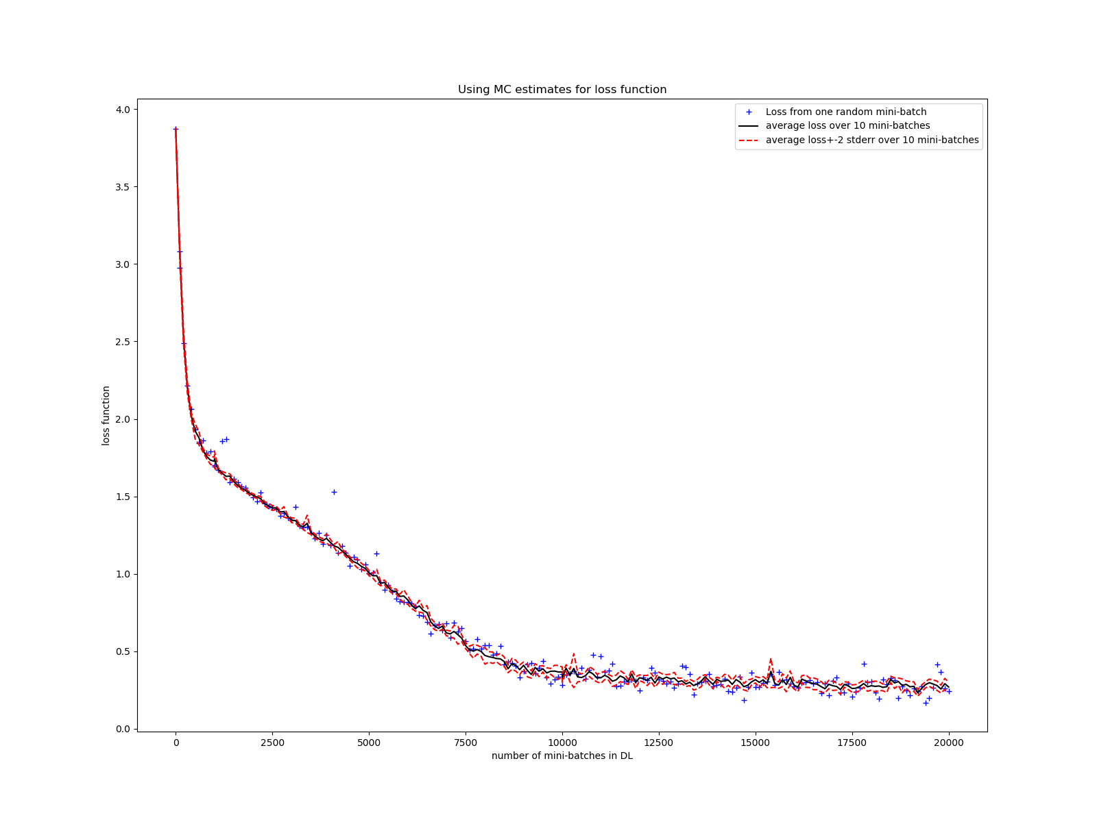
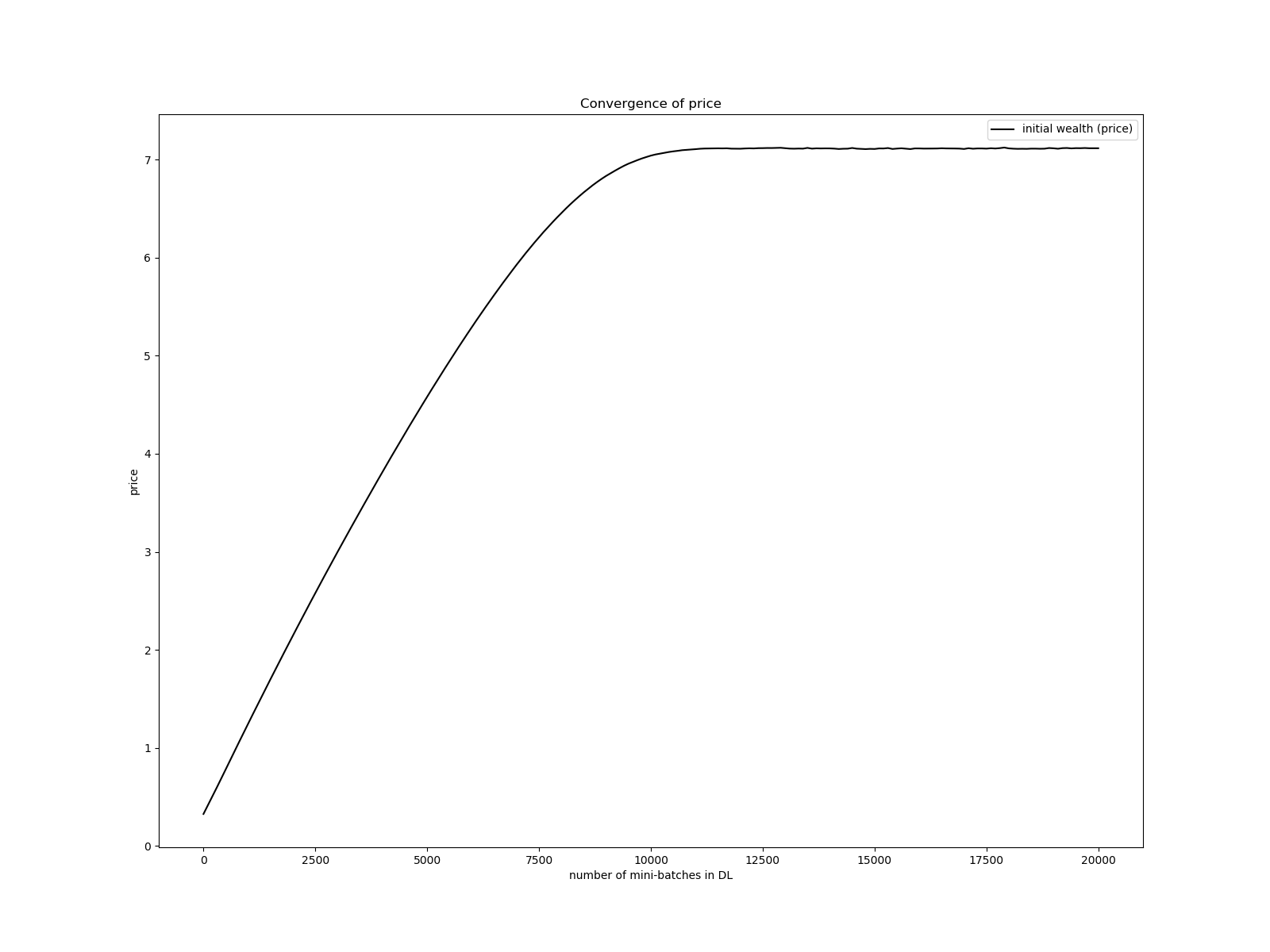
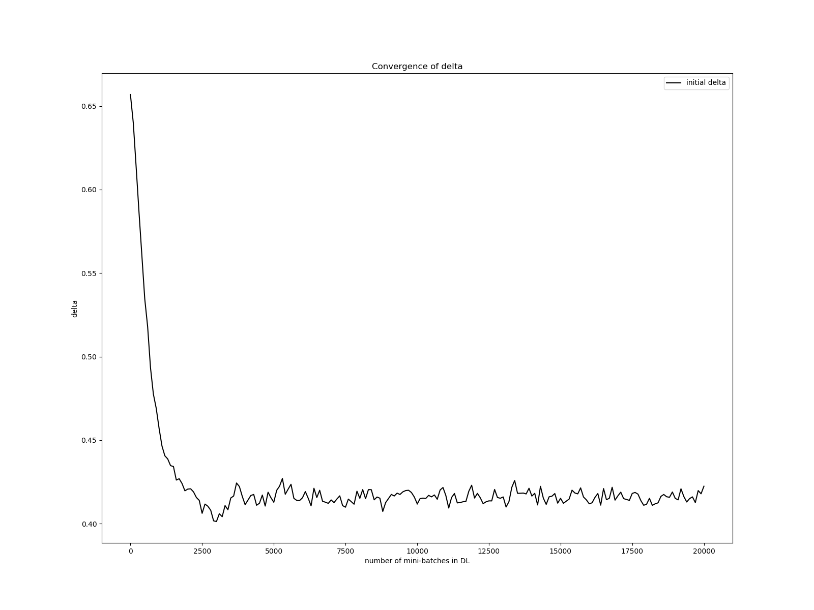
Figure 3: Forward method with fixed initial risk factor values. Upper: loss function/functional over mini-batch number. Lower-left: convergence of price. Lower-right: convergence of delta.

Now for the variant with random initial risk factors: Figure 4 shows that the loss functional decays quite quickly for this case also, that the final payoff is well replicated, that the analytical solution is well approximated, the delta is quite well approximated as well (considering that we only hedge at discrete times and not continuously), and that the $Y$ surface and the portfolio functions surface looks well-defined and smooth.

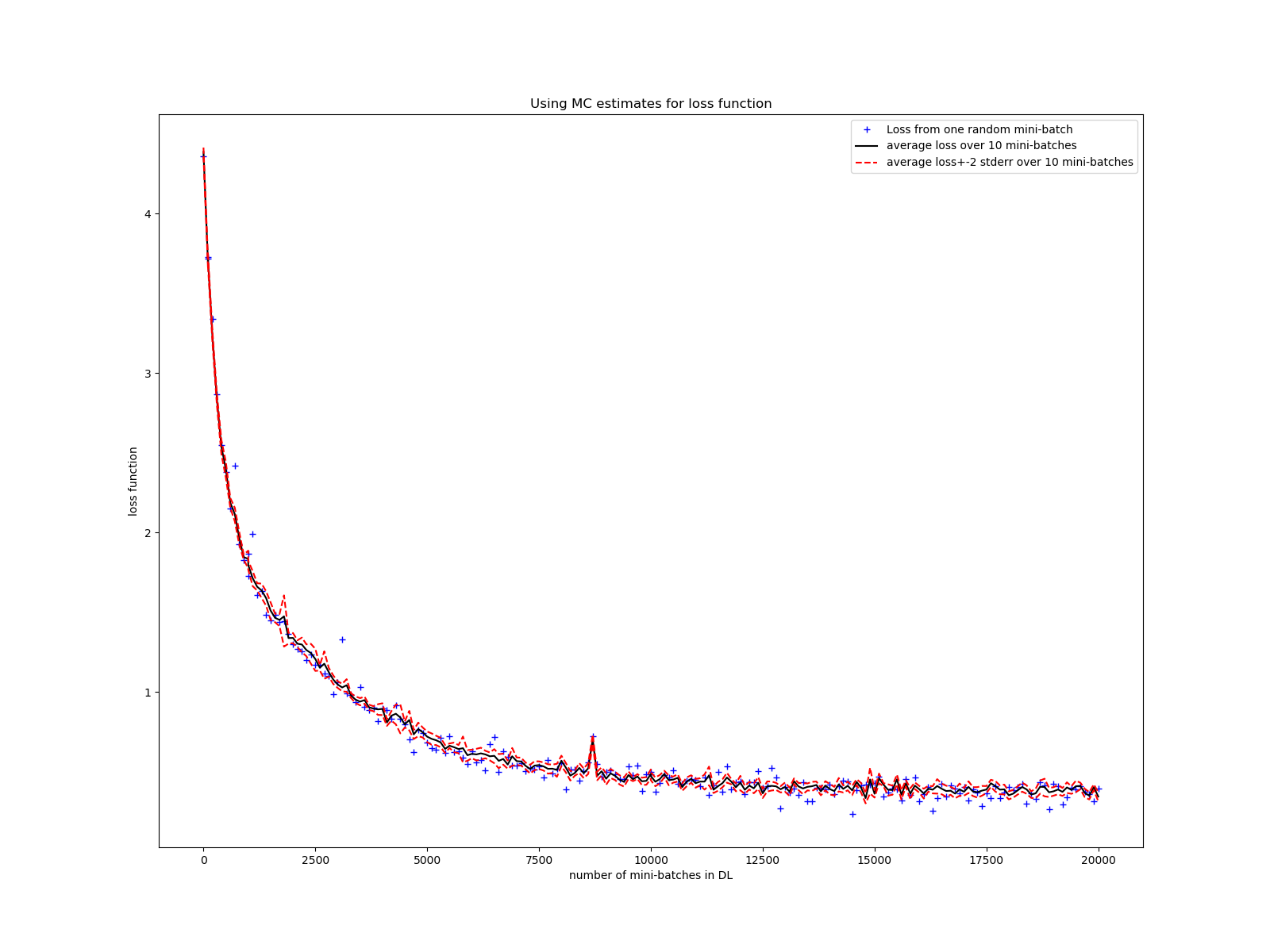
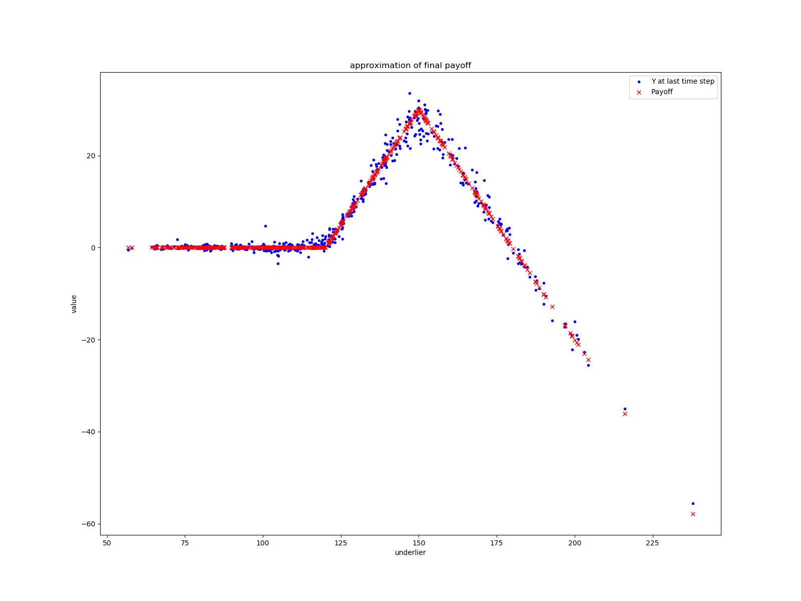
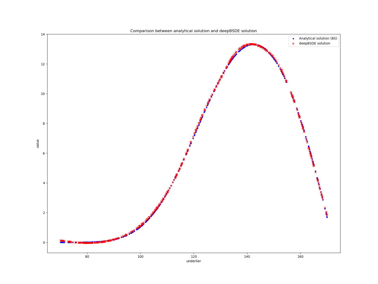
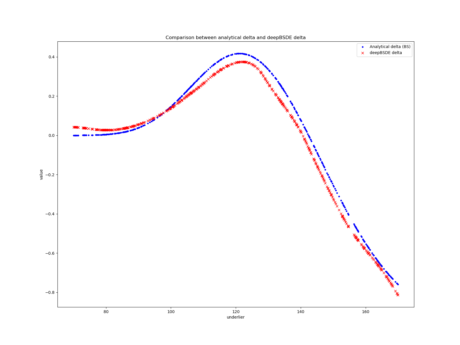
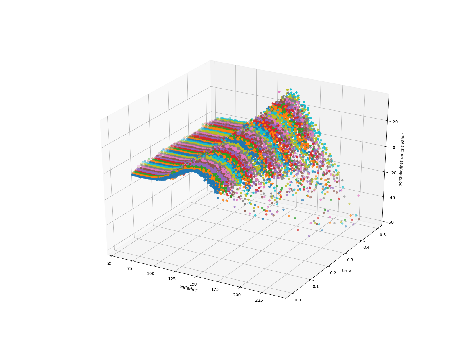
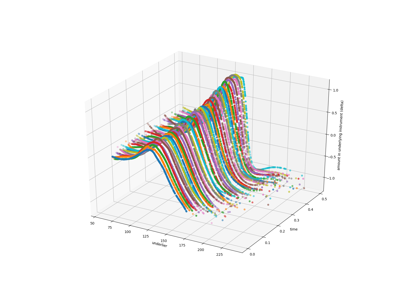
Figure 4: Forward method with random initial risk factor values. Upper-left: Loss function/functional over mini-batch number. Upper-right: Final Payoff match at 20000. Middle-left: comparison of initial $Y$ network and analytical solution. Middle-right: comparison of initial portfolio delta and analytical delta. Lower-left: scatter plot of $Y$. Lower-right: scatter plot of $\Pi$.

9.2 Backward methods

First, some results for the variant with fixed initial risk factors. Figure 5 shows that the loss functional decays quite quickly as a function of number of mini-batches run and how price and delta at fixed initial risk factor (“spot”) converge up to good accuracy. (In this case, we actually trained $\Pi$ networks with shared parameters - which means that the network also has $t$ as an input.) We see that the backward method seems to converge faster than the forward method in this case.

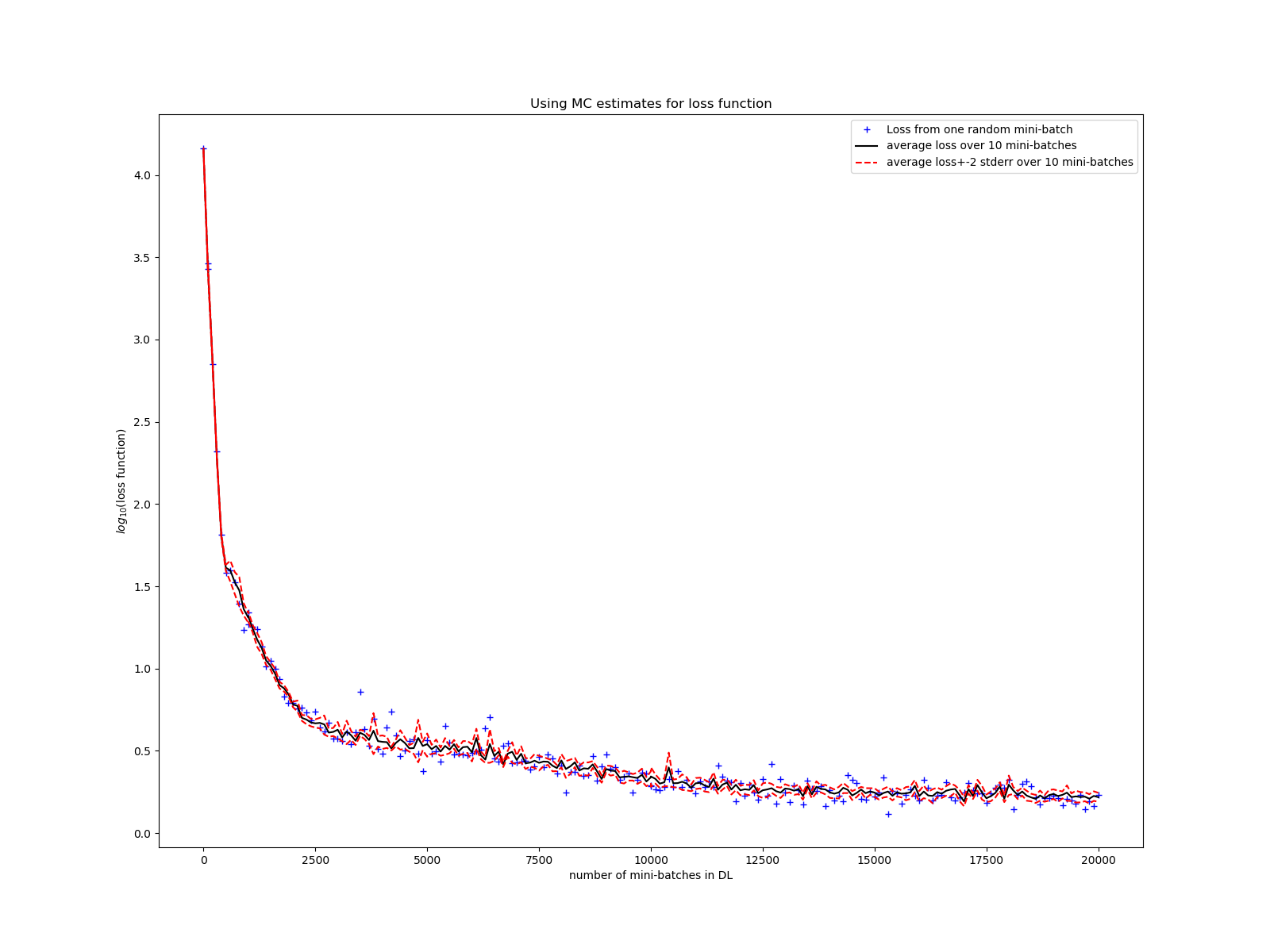
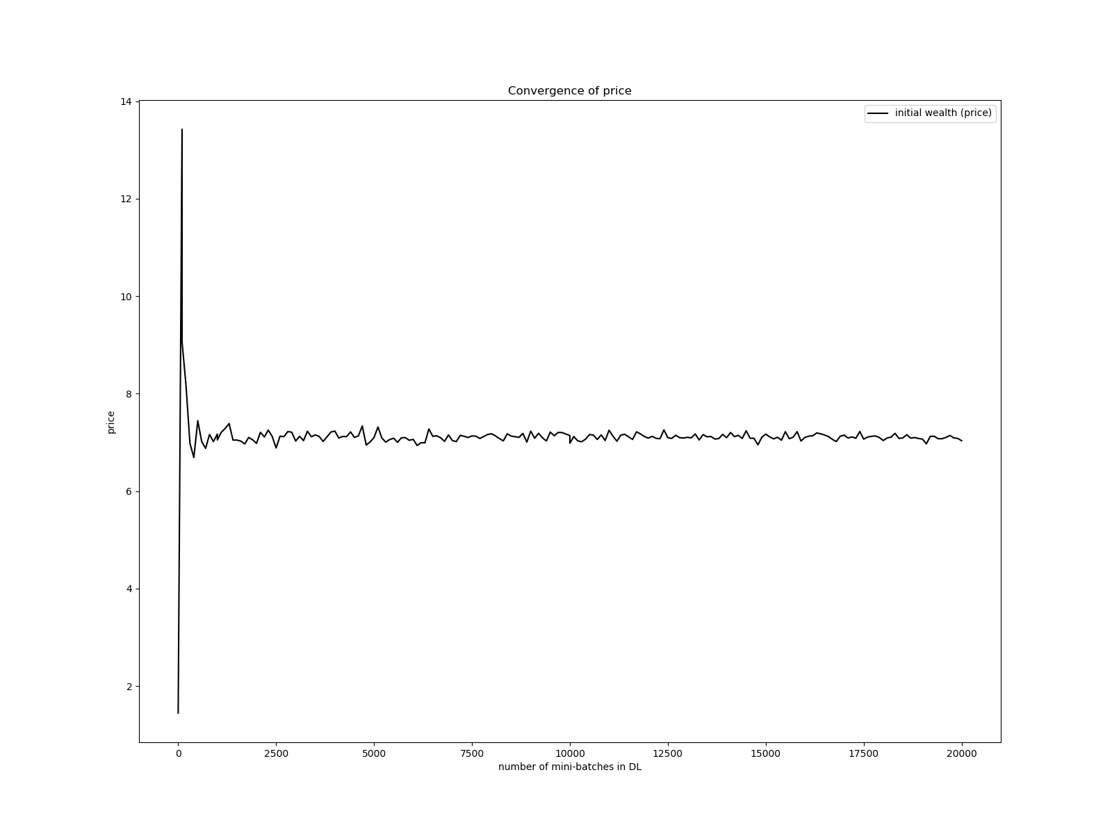
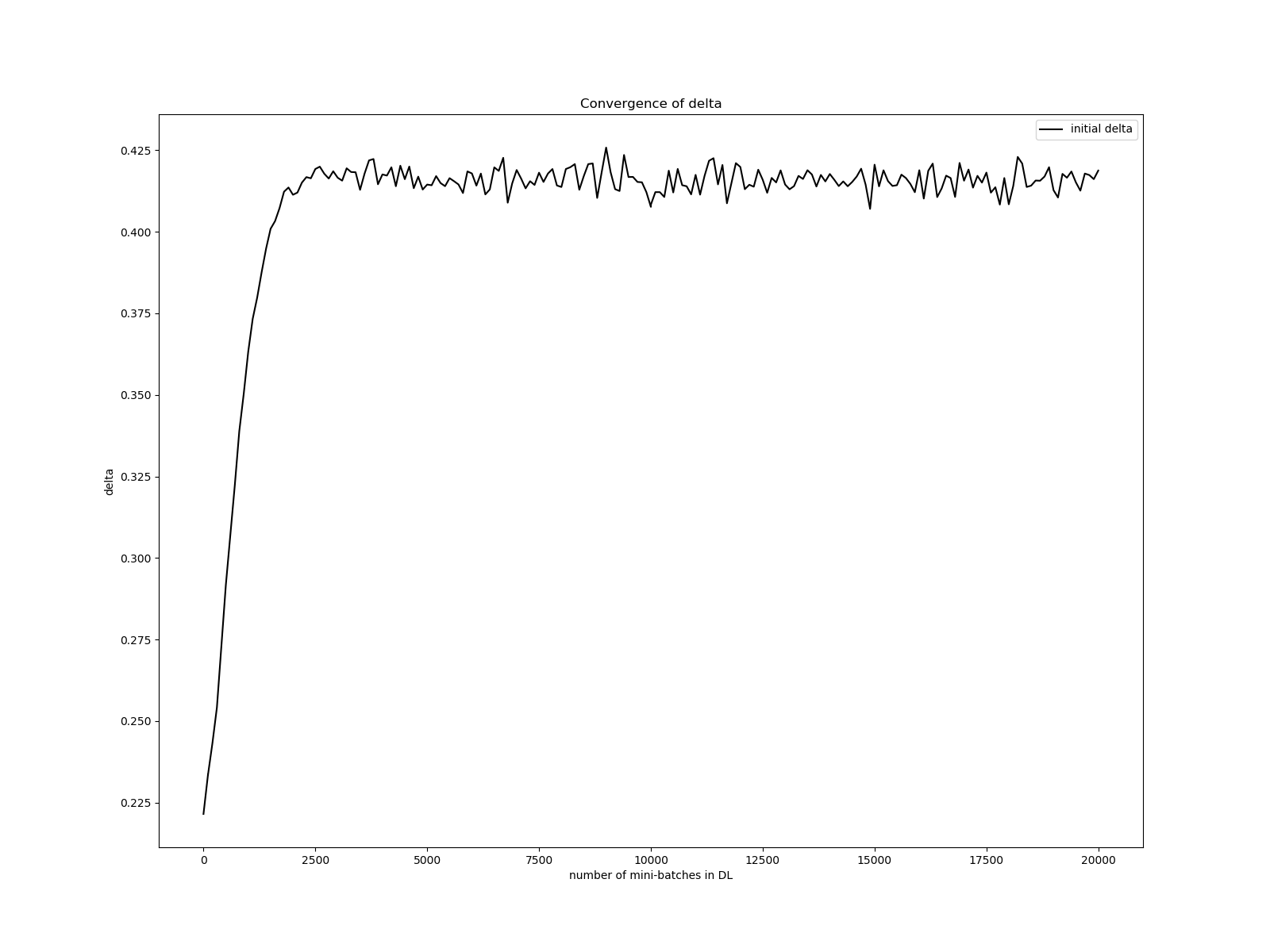
Figure 5: Backward method with fixed initial risk factor values. Upper: loss function/functional over mini-batch number. Lower-left: convergence of price. Lower-right: convergence of delta.

Now for the variant with random initial risk factors: Figure 6 shows that the loss functional decays quite quickly for this case also, that the analytical initial solution is well approximated and that the rolled-back $Y_{0}$ are concentrated around the initial solution and network, the delta is quite well approximated as well (considering that we only hedge at discrete times and not continuously), and that the $Y$ surface and the portfolio functions surface looks well-defined and smooth.

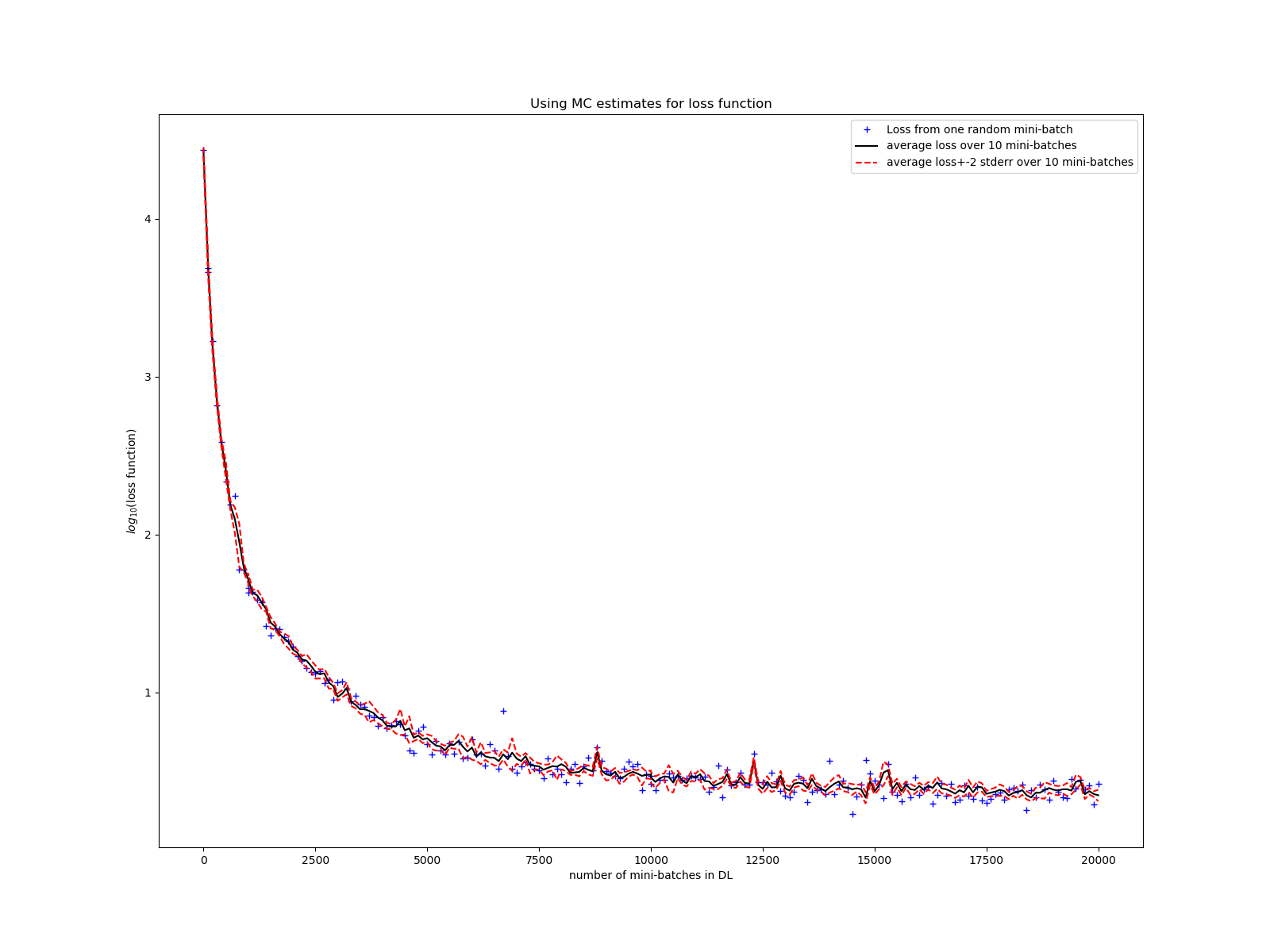
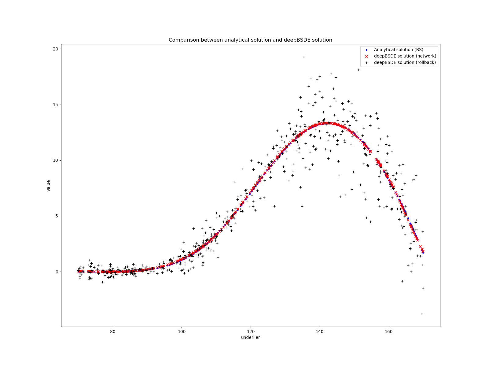
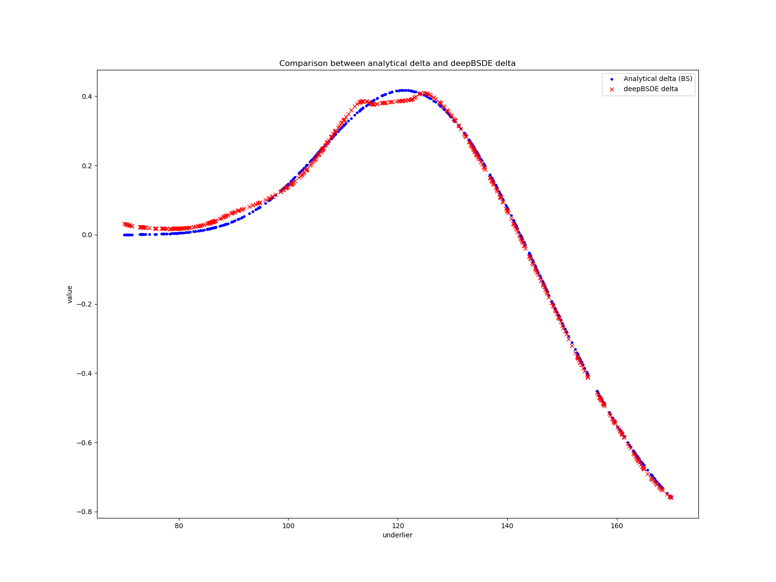
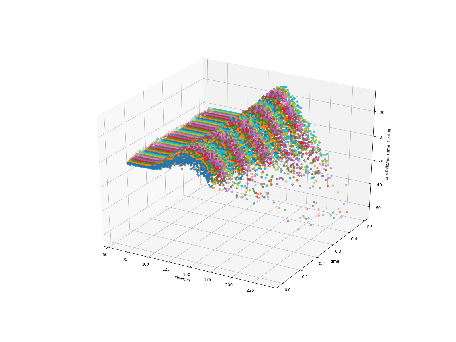
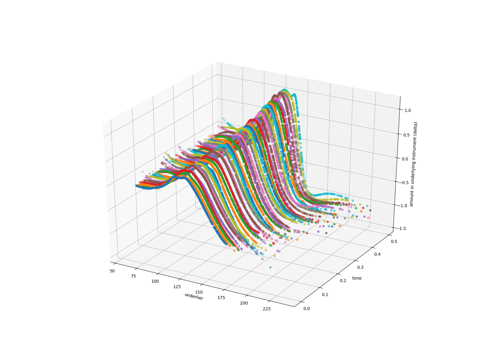
Figure 6: Backward method with random initial risk factor values. Upper: Loss function/functional over mini-batch number. Middle-left: comparison of initial $Y$ network, rolled-back $Y_{0}$, and analytical solution. Middle-right: comparison of initial portfolio delta and analytical delta. Lower-left: scatter plot of $Y$. Lower-right: scatter plot of $\Pi$.

10 Conclusion

We demonstrated how a wide variety of modeling approaches in quantitative finance for European, Barrier, and Bermudan option pricing can be solved through deep learning optimization approaches for the forward-backward stochastic differential equation (FBSDE) formulations where the forward and the backward SDE are time-stepped to simulate pathwise values and showed examples for European option pricing for both the forward and backward approaches.

References

- [CWNMW19] Quentin Chan-Wai-Nam, Joseph Mikael, and Xavier Warin. Machine learning for semi linear PDEs. Journal of Scientific Computing, 79(3):1667–1712, 2019. arXiv:1809.07609.
- [EHJ17] Weinan E, Jiequn Han, and Arnulf Jentzen. Deep learning-based numerical methods for high-dimensional parabolic partial differential equations and backward stochastic differential equations. Communications in Mathematics and Statistics, 5(4):349–380, 2017. arXiv:1706.04702.
- [EKPQ97] Nicole El Karoui, Shige Peng, and Marie Claire Quenez. Backward stochastic differential equations in finance. Mathematical finance, 7(1):1–71, 1997. Also available on semanticscholar.org.
- [GMKS19] Lukas Gonon, Johannes Muhle-Karbe, and Xiaofei Shi. Asset pricing with general transaction costs: Theory and numerics. arXiv preprint arXiv:1905.05027, 2019.
- [HJE18] Jiequn Han, Arnulf Jentzen, and Weinan E. Solving high-dimensional partial differential equations using deep learning. Proceedings of the National Academy of Sciences, 115(34):8505–8510, 2018.
- [IS15] Sergey Ioffe and Christian Szegedy. Batch normalization: Accelerating deep network training by reducing internal covariate shift. arXiv preprint arXiv:1502.03167, 2015.
- [KB14] Diederik P Kingma and Jimmy Ba. Adam: A method for stochastic optimization. arXiv preprint arXiv:1412.6980, 2014.
- [LXL19] Jian Liang, Zhe Xu, and Peter Li. Deep learning-based least square forward-backward stochastic differential equation solver for high-dimensional derivative pricing. arXiv preprint arXiv:1907.10578, 2019. Also available at SSRN: https://ssrn.com/abstract=3381794 or http://dx.doi.org/10.2139/ssrn.3381794.
- [Per10] Nicolas Perkowski. Backward Stochastic Differential Eequations: an Introduction, 2010. Available on semanticscholar.org.
- [WCS+18] Haojie Wang, Han Chen, Agus Sudjianto, Richard Liu, and Qi Shen. Deep learning-based BSDE solver for LIBOR market model with application to bermudan swaption pricing and hedging. arXiv preprint arXiv:1807.06622, 2018. Also available at SSRN: https://ssrn.com/abstract=3214596 or http://dx.doi.org/10.2139/ssrn.3214596.
- [YXS19] Bing Yu, Xiaojing Xing, and Agus Sudjianto. Deep-learning based numerical BSDE method for Barrier options. arXiv preprint arXiv:1904.05921, 2019. Also available at SSRN: https://ssrn.com/abstract=3366314 or http://dx.doi.org/10.2139/ssrn.3366314.