Causality, unitarity, and indefinite metric in Maxwell-Chern-Simons extensions

Abstract

We canonically quantize $(2+1)$-dimensional electrodynamics including a higher-derivative Chern-Simons term. The effective theory describes a standard photon and an additional degree of freedom associated with a massive ghost. We find the Hamiltonian and the algebra satisfied by the field operators. The theory is characterized by an indefinite metric in the Hilbert space that brings up questions on causality and unitarity. We study both of the latter fundamental properties and show that microcausality as well as perturbative unitarity up to one-loop order are conserved when the Lee-Wick prescription is employed.

I Introduction

The concept of an indefinite metric in a Hilbert space plays a fundamental role in the formulation of relativistic quantum field theory. Dirac was the first to show how an indefinite metric arises in quantum electrodynamics and proposed how to deal with its probability interpretation Dirac . One can mention two reasons for Dirac’s suggestion. On the one hand, any finite representation of a noncompact group — the Lorentz group included — leads to a state space endowed with an indefinite metric. On the other hand, the commutator of two vector field operators reads

$$[A_{\mu}(x),A_{\nu}(y)]=\mathrm{i}\eta_{\mu\nu}D(x-y)\,,$$ (1)

with the scalar commutator function $D$ and the Minkowski metric $\eta_{\mu\nu}$. The difference in the signs of the metric components $\eta_{00}$ and $\eta_{ii}$ induces an indefinite metric in the corresponding state space; see, in particular, Heisenberg’s contribution in the list of references Aspects ; Heisenberg2 ; Pauli .

Gupta and Bleuler used this concept within the covariant quantization of electrodynamics. The Gupta-Bleuler formalism shows that the unphysical degrees of freedom are eliminated by imposing the weak Lorentz condition on the Hilbert space. Many of the motivations for studying indefinite metric theories come from the theory of gravitation, where the nonrenormalizability of the Einstein-Hilbert action forces one to consider the possibility of modified gravity theories. Some of them also introduce indefinite metrics in the Hilbert space Stelle ; Nakanishi-QFT ; Nakanishi-GR .

The most notorious drawback of indefinite-metric theories is the possibility of negative probabilities leading to the loss of unitarity. Unitarity in this context has been studied extensively for the past decades. In the sixties, Lee and Wick, being attracted by the idea of reconciling the divergencies in quantum electrodynamics (QED) without spoiling unitarity, constructed a modified electrodynamics with an indefinite metric. Their theory, which is known as Lee-Wick model Lee-Wick:Negative ; Lee-Wick:Finite , is a modified electrodynamics including a massive boson field associated with negative metric components. One characteristic of the propagator of their theory is that it contains complex conjugate pairs of additional poles, which are called Lee-Wick poles.

The Lee-Wick model is also obtained by introducing a higher-derivative term in the Lagrangian Exploring . In this model, perturbative unitarity of the $S$-matrix has been successfully implemented via the Cutkosky-Landshoff-Olive-Polkinghorne prescription in which a pair of Lee-Wick poles cancel each other in cut diagrams Anon-analytic . Several approaches have provided a deeper understanding of many physical aspects of Lee-Wick models in the last years TheLee-Wick ; Fior ; Anewformulation ; Perturbativeunitarity . In fact, investigations aimed at providing finiteness in quantum field theory have not stopped, reaching diverse application within nonlocal quantum gravity; see, e.g., loop ; Super-Lee-Wick ; Briscese and higher-derivative gravity extensions studied even earlier Stelle .

Basically, the loss of unitarity occurs due to the negative contribution of the residue of the ghost field to scattering cross sections. In this case the cutting equations provided by the optical theorem cannot be satisfied. It was demonstrated that one can modify the definition of the internal product in the Hilbert space in order to cope with the unitarity problem. However, this approach leads to theories characterized by non-Hermitian Hamiltonians, i.e., they exhibit a nonstandard time evolution. However, Bender and collaborators found that such Hamiltonians have real eigenvalues when they are symmetric under $\mathit{PT}$ transformations Bender . Scenarios of this kind have attracted an exceeding interest, see, e.g., Fring ; Alexandre where non-Hermitian Hamiltonians are discussed, too.

Another motivation for the interest in indefinite metric theories originated from gravity where it was demonstrated that adding higher-derivative terms allows for gravity to be renormalizable Stelle . This fact implied active studies of renormalization of $R^{2}$ gravity and other higher-derivative gravity theories (see, e.g., Asorey and references therein). Nevertheless, it was realized soon that this kind of improvement of the renormalization behavior inevitably leads to ghosts. From the formal viewpoint, their presence can be explained as follows. Consider the example of a propagator $\frac{1}{k^{2}(k^{2}+m^{2})}$ occurring in a fourth-derivative theory. A simple transformation shows that this propagator describes two particles: a massless and a massive one. The propagator of the latter carries a negative sign, whereby the massive particle corresponds to a free scalar field with possibly negative energy. Even if the energy in the theory can be bounded from below due to a redefinition of vacuum, unitarity, upon the presence of interactions, is expected to be broken (see HH ; E-W for more detailed explanations).

Furthermore, more problems related to the consistent quantum description of higher-derivative theories were discussed in Ant ; Anewformulation ; Perturbativeunitarity . In the latter papers, it was claimed that these problems actually arise due to differences between the behaviors of the theory in Minkowski spacetime and its counterpart in Euclidean space. At the same time, it was argued in Smilga that in certain cases the ghosts are “benign” so that the theory turns out to be perturbatively unitary, with the vacuum being perturbatively stable. Therefore, the problem of ghosts must be considered separately for any higher-derivative theory.

An interesting example of a higher-derivative extension of quantum electrodynamics (QED) containing dimension-five operators was proposed by Myers and Pospelov MP . The higher-derivative term in its Lagrangian, called the Myers-Pospelov term, involves explicit Lorentz symmetry breaking, so that for some special choice of the Lorentz-breaking preferred four-vector, higher time derivatives do not arise, whereupon unitarity breaking is avoided. In case an indefinite metric occurs, one can apply the Lee-Wick prescription to show that unitarity is conserved tree1 ; loop1 ; Unit_loop . According to the latter, all negative-norm states are removed from the asymptotic Hilbert space. This procedure will turn out to be fruitful in the analysis that we intend to carry out in the current paper.

A further interesting Lorentz-breaking modification of QED is the higher-derivative Carroll-Field-Jackiw-like term exhibiting a similar behavior (both of these terms were shown to be generated perturbatively at the one-loop level, whereby the corresponding contributions are finite, see MNP ). In a different context, though, the possibility of Lorentz violation due to an indefinite metric was pointed out several years ago by Nakanishi LIV-LW ; Nakanishi-LIV .

Therefore, to understand the physical impact of effective higher-derivative extensions of QED, it is important to check how such terms affect unitarity. To do so, though, it is reasonable to investigate a simplified model first, that is, $(2+1)$-dimensional QED with an additive higher-derivative Chern-Simons (CS) term, which does not involve Lorentz symmetry breaking. Some classical issues related to this theory such as the nature and behavior of degrees of freedom were analyzed earlier in DJ . Its canonical formulation was discussed in testing and the perturbative generation of the higher-derivative CS term was carried out in Passos . Here, we intend to elaborate on the aspects of microcausality and unitarity of this theory.

The structure of the paper looks as follows. In Sec. II, we introduce the classical action and the propagator of our theory, write down the classical field equations, the dispersion equation, and its solutions. Furthermore, we decompose the higher-derivative theory into a standard one involving degrees of freedom associated with a three-component photon field and a second contribution in terms of a Proca ghost field. We then find the polarization vectors for the photon and the massive ghost as well as their stress tensors. In Sec. III, we canonically quantize the theory, construct the field operators such that they satisfy the expected algebra, and analyze the constraint structure in combination with finding the Hamiltonian. In Sec. IV, we verify tree-level unitarity of our theory and we also study perturbative unitarity at one-loop level. Section V states a final summary and discussion of our results. Appendix A contains details of the derivation of Dirac brackets and the Dirac formalism that reduces second-class constraints to zero. Appendix B explains how to express the Hamiltonian of the theory in terms of creation and annihilation operators. Appendix C delivers detailed computations of the nonzero equal-time commutators satisfied by the field operators. Finally, appendix D provides a summary of the most important properties of a Dirac theory in $(2+1)$ dimensions.

II Higher-derivative Maxwell-Chern-Simons theory

In this section, we present the higher-derivative CS term coupled to the Maxwell Lagrangian in $(2+1)$ dimensions. The theory describes a standard photon and a massive mode at high energies associated with a ghost. To show this, we apply a linear transformation to the higher-derivative Lagrangian decoupling it into a sum of two standard-derivative parts. We find the polarization vectors and connect their sum with the propagator, which simplifies the study of unitarity in Sec. IV.

II.1 The $(2+1)$-dimensional model

Our starting point consists of a Lagrangian that is the sum of the standard Maxwell term and the higher-derivative CS extension in $(2+1)$ dimensions DJ , given by

$$\mathcal{L}=-\frac{1}{4}F_{\mu\nu}F^{\mu\nu}+\frac{g}{2}\epsilon^{\alpha\beta\gamma}(\Box A_{\alpha})(\partial_{\beta}A_{\gamma})+\mathcal{L}_{\mathrm{GF}}\,,$$ (2)

where $\square=\partial^{\mu}\partial_{\mu}$ is the d’Alembertian and $g$ is a small constant with inverse mass dimension. We will see that the inverse of $g$ is related to a mass scale. Thus, it is assumed that $g>0$. Furthermore, $\mathcal{L}_{\mathrm{GF}}$ is a covariant gauge-fixing term inversely proportional to the arbitrary gauge-fixing parameter $\xi$

$$\mathcal{L}_{\mathrm{GF}}=-\frac{1}{2\xi}(\partial_{\mu}A^{\mu})^{2}\,.$$ (3)

We take the metric convention $\eta_{\mu\nu}=\text{diag}(+,-,-)$, and our definition of the Levi-Civita symbol is based on $\epsilon^{012}=\epsilon_{012}=\epsilon^{12}=\epsilon_{12}=1$. Hence, all Lorentz indices run over 0,1,2.

Within our study we do not consider the usual single-derivative CS term for the sake of simplicity, since we aim at keeping track of the higher-derivative contribution. We note that the CS term is suppressed above some energy scale in comparison to our higher-derivative term. In principle, though, it is natural to expect that it would not render the physics essentially different. Nevertheless, the complete analysis of unitarity and, especially, of the Dirac algebra of constraints will be much more involved if the CS term is present. Therefore, we discard it in our analysis.

We note in passing that a $(2+1)$-dimensional Lorentz-violating electromagnetism involving higher-derivative terms was derived in Ferreira:2019jbx from the electromagnetic sector of the nonminimal Standard-Model Extension Kostelecky:2009zp via a procedure known as dimensional reduction (see, e.g., Belich:2002vd ; Belich:2003xa ). The second contribution in Eq. (2) can be mapped onto the third one in $\mathcal{L}_{(1+2)}$ of Ferreira:2019jbx via suitable partial integrations.

The treatment of systems in classical mechanics described by higher-derivative Lagrangians was initiated by Ostrogradsky in his seminal paper Ostro . Subsequent scientific papers reviewing and extending his original ideas are Borneas:1959 ; Riahi:1972 ; Woodard:2015 where this list is not claimed to be exhaustive. One of the central results of these works is that an application of the Hamilton principle leads to a modified set of Euler-Lagrange equations. An analogous development of the formalism in the context of higher-derivative field theory can be found, e.g., in Bollini:1986am . For the particular field theory defined by Eq. (2), it is sufficient to restrict these generalized Euler-Lagrange equations to

$$-\partial_{\kappa}\partial_{\lambda}\frac{\partial\mathcal{L}}{\partial(\partial_{\kappa}\partial_{\lambda}A_{\sigma})}+\partial_{\rho}\frac{\partial\mathcal{L}}{\partial(\partial_{\rho}A_{\sigma})}-\frac{\partial\mathcal{L}}{\partial A_{\sigma}}=0\,.$$ (4)

They lead to the modified Maxwell equations

$$\partial_{\rho}F^{\rho\sigma}+g\epsilon^{\sigma\beta\gamma}\Box\partial_{\beta}{A}_{\gamma}+\frac{1}{\xi}\partial^{\sigma}(\partial\cdot A)=0\,.$$ (5)

Now, contracting Eq. (5) with $\partial_{\sigma}$ yields

$$\frac{1}{\xi}\Box\left(\partial\cdot A\right)=0\,.$$ (6)

Hence, by imposing suitable boundary conditions at infinity it follows that $\partial\cdot A=0$ can be set.

Now, let us rewrite the Lagrangian (2) as

$$\mathcal{L}=\frac{1}{2}A_{\mu}\left[\Box\eta^{\mu\nu}-\left(1-\frac{1}{\xi}\right)\partial^{\mu}\partial^{\nu}+g\epsilon^{\mu\beta\nu}\partial_{\beta}\Box\right]A_{\nu}\,,$$ (7)

yielding the equations of motion for the gauge field:

$$\left[\Box\eta^{\mu\nu}-\left(1-\frac{1}{\xi}\right)\partial^{\mu}\partial^{\nu}+g\epsilon^{\mu\beta\nu}\partial_{\beta}\Box\right]A_{\nu}(x)=0\,.$$ (8)

Transforming the latter to the momentum representation with $\mathrm{i}\partial_{\mu}=p_{\mu}$, we write

$$S^{\mu\nu}(p)A_{\nu}(p)=0\,,$$ (9a)

with

$$S^{\mu\nu}(p)=p^{2}\left[\eta^{\mu\nu}-\left(1-\frac{1}{\xi}\right)\frac{p^{\mu}p^{\nu}}{p^{2}}-\mathrm{i}g\epsilon^{\mu\beta\nu}p_{\beta}\right]\,.$$ (9b)

The propagator $P_{\mu\nu}$ follows from inverting the operator $S^{\mu\nu}$, giving

$$P_{\mu\nu}(p)=-\frac{G_{\mu\nu}(\xi,p)}{p^{2}(1-g^{2}p^{2})}\,,$$ (10a)

where

$$G_{\mu\nu}(\xi,p)=\eta_{\mu\nu}-\left[1-\xi\left(1-g^{2}p^{2}\right)\right]\frac{p_{\mu}p_{\nu}}{p^{2}}+\mathrm{i}g\epsilon_{\mu\beta\nu}p^{\beta}\,.$$ (10b)

The conventions have been chosen such that the propagator satisfies

$$S^{\mu\nu}(p)P_{\nu\rho}(p)=-\delta^{\mu}_{\phantom{\mu}\rho}\,.$$ (11)

Considering the pole structure of the propagator (10) and defining $g\equiv M^{-1}$, we decompose the denominator as

$$\frac{M^{2}}{p^{2}(p^{2}-M^{2})}=-\frac{1}{p^{2}}+\frac{1}{p^{2}-M^{2}}\,,$$ (12)

where the second contribution has a residue whose sign is opposite to that of the first contribution. Hence, it can be associated with a ghost. The dispersion relations are given by the propagator poles with respect to $p_{0}$. Determining the poles yields the modes corresponding to a photon and a massive gauge field given by

$$\omega(\vec{p}) =\omega_{p}= |\vec{p}|\,,$$ (13a)

$$\Omega(\vec{p}) =\Omega_{p}= \sqrt{\vec{p}^{\,2}+M^{2}}\,,$$ (13b)

respectively.

Let us write down the energy-momentum tensor of our theory. It is clear that it is a sum of two contributions. The first is the energy-momentum tensor for electrodynamics in $(2+1)$ dimensions whose symmetric form is the well-known Belinfante tensor equal to

$$T_{\mathrm{Bel}}^{\mu\nu}=F^{\mu}_{\phantom{\mu}\lambda}F^{\lambda\nu}+\frac{1}{4}\eta^{\mu\nu}F_{\alpha\beta}F^{\alpha\beta}\,.$$ (14)

The second is connected to the higher-derivative Chern-Simons (HDCS) theory, whose symmetric form was found explicitly in DJ . So we merely quote the result, which is

$$T^{\mu\nu}_{\mathrm{HDCS}}=g[(\epsilon^{\mu\alpha\beta}F^{\ast\nu}+\epsilon^{\nu\alpha\beta}F^{\ast\mu})\partial_{\alpha}F^{\ast}_{\beta}-\eta^{\mu\nu}\epsilon^{\alpha\beta\gamma}F^{\ast}_{\alpha}\partial_{\beta}F^{\ast}_{\gamma}],$$ (15)

where $F^{\ast}_{\alpha}=\frac{1}{2}\epsilon_{\alpha\mu\nu}F^{\mu\nu}$ is the dual of the field strength tensor $F^{\mu\nu}$.

II.2 Decoupling the ghost

Here we make explicit the two types of fields described by the Lagrangian (2). We define the new fields as

$${\bar{A}}_{\mu} = \frac{1}{\sqrt{2}}(A_{\mu}+gF^{\ast}_{\mu})\,,$$ (16a)

$${G}_{\mu} = \frac{g}{\sqrt{2}}F^{\ast}_{\mu}\,,$$ (16b)

in terms of the dual tensor $F_{\mu}^{\ast}$ defined under Eq. (15) and the original photon field $A_{\mu}$.

Considering Eqs. (16a) and (16b), we find the identities

$$-\frac{1}{4}\bar{F}_{\mu\nu}\bar{F}^{\mu\nu} =-\frac{1}{8}F_{\mu\nu}F^{\mu\nu}$$

$$\phantom{{}={}}-\frac{g}{2}\left(\partial_{\mu}A_{\nu}+\frac{g}{2}\partial_{\mu}F^{\ast}_{\nu}\right)(\partial^{\mu}F^{\ast\nu}-\partial^{\nu}F^{\ast\mu})\,,$$ (17a)

and

$$-\frac{1}{4}F^{\ast}_{\mu}F^{\ast\mu}=-\frac{1}{8}F_{\mu\nu}F^{\mu\nu}\,,$$ (17b)

where $\bar{F}_{\mu\nu}=\partial_{\mu}\bar{A}_{\nu}-\partial_{\nu}\bar{A}_{\mu}$ is the field strength tensor associated with the new field of Eq. (16a).

Now, by adding both equations, performing suitable integrations by parts, and using the (unmodified) homogeneous Maxwell equation $\partial_{\mu}F^{*\mu}=0$ in $(2+1)$ dimensions, we can rewrite the first part of the Lagrangian (2) as

$$-\frac{1}{4}F_{\mu\nu}F^{\mu\nu}+\frac{g}{2}\epsilon^{\alpha\beta\gamma}(\Box A_{\alpha})(\partial_{\beta}A_{\gamma})$$

$$=-\frac{1}{4}\bar{F}_{\mu\nu}\bar{F}^{\mu\nu}-\frac{g^{2}}{4}F^{\ast}_{\mu}\left(\frac{1}{g^{2}}+\Box\right)F^{\ast\mu}\,.$$ (18)

Using the definition (16b) and $\partial_{\mu}{A^{\mu}}=\sqrt{2}\,\partial_{\mu}{\bar{A}^{\mu}}$ allows us to write the higher-derivative Lagrangian as the sum

$$\mathcal{L} =-\frac{1}{4}\bar{F}_{\mu\nu}\bar{F}^{\mu\nu}-\frac{1}{\xi}(\partial_{\mu}\bar{A}^{\mu})^{2}$$

$$\phantom{{}={}}+\frac{1}{2}\partial_{\mu}{G}_{\nu}\partial^{\mu}{G}^{\nu}-\frac{1}{2}M^{2}{G}_{\mu}{G}^{\mu}\,,$$ (19)

where the higher derivatives have been absorbed into the new fields. The first part of the new Lagrange density describes a photon with a gauge fixing term and the second part corresponds to a Proca field theory involving a mass scale of the order of $M\sim g^{-1}$. As the coupling constant $g$ of the modification is assumed to be small, the latter mass scale $M$ is supposed to be large. The Proca field theory presumably describes a ghost dominating the regime of high energies.

II.3 Polarization vectors

Now that the theory has been decomposed into two decoupled standard-derivative parts associated with the fields of Eqs. (16a) and (16b), our next step is to find the polarization vectors. First, they are crucial for the computation of the Hamiltonian in terms of creation and annihilation operators. Second, they are needed to construct the tensor structure in the equal-time commutation relations of the field operators. Last but not least, the propagator can be expressed in terms of the polarization vectors, which will be helpful to prove the validity of the optical theorem.

To begin with, consider the following orthogonal basis of $(2+1)$-dimensional Minkowski spacetime that involves the three real vectors

$$e^{(0)\mu} =\frac{1}{\sqrt{p^{2}}}p^{\mu},$$ (20a)

$$e^{(1)\mu} =\frac{1}{\sqrt{G}}\epsilon^{\mu\beta\gamma}p_{\beta}n_{\gamma},$$ (20b)

$$e^{(2)\mu} =-\frac{1}{\sqrt{p^{2}}}\epsilon^{\mu\beta\gamma}p_{\beta}e^{(1)}_{\gamma}=\frac{1}{\sqrt{p^{2}G}}(p^{2}n^{\mu}-p^{\mu}(p\cdot n)),$$ (20c)

where $G=(p\cdot n)^{2}-p^{2}n^{2}$ and $n^{\mu}$ is an auxiliary three-vector. The three-vectors $e^{(a)}_{\mu}$ are normalized according to

$$e^{(a)}\cdot e^{(b)}=g_{ab}\,,$$ (21)

with $a=0,1,2$ and $g_{ab}=\text{diag}(1,-1,-1)$. Although $g_{ab}$ formally corresponds to the Minkowski metric in $(2+1)$ dimensions, we use another symbol here, as the indices of this object are not Lorentz indices, but merely the labels of the vectors introduced before. In order to ensure $G>0$, we will take $p^{2}>0$ and choose $n^{\mu}$ as a timelike vector.

Furthermore, these vectors satisfy the completeness relation

$$\sum_{a,b=0}^{2}g_{ab}\,e^{(a)}_{\mu}e^{(b)}_{\nu}=\eta_{\mu\nu}\,.$$ (22)

However, note that the above basis is not suitable to describe the photon field due to the denominator depending on $\sqrt{p^{2}}$. To construct suitable polarization vectors for photons we will proceed differently in the subsection III.1.

Moreover, one can check that the $e^{(a)}_{\mu}$ fulfill the relations

$$\epsilon^{\mu\beta\gamma}p_{\beta}e^{(2)}_{\gamma} = \sqrt{p^{2}}e^{(1)\mu}\,,$$ (23a)

$$\epsilon^{\mu\beta\gamma}p_{\beta}e^{(1)}_{\gamma} = -\sqrt{p^{2}}e^{(2)\mu}\,.$$ (23b)

With the real basis $\{e^{(a)}\}$ at hand, we look for a complex basis $\{\varepsilon^{(\lambda)}\}$ diagonalizing the operator $S^{\mu}_{\phantom{\mu}\nu}(p)$ of Eq. (9b). Our intention is to relate the propagator to the sum of polarization tensors formed from the vectors of $\{\varepsilon^{(\lambda)}\}$. This particular method was introduced in CMP and applied in the context of the Maxwell-Chern-Simons-like theory in $(3+1)$ dimensions. We adopt it to the theory of Eq. (2), as it turned out to be valuable for checking the validity of the optical theorem. Hence, considering Eq. (9b) we demand that these vectors fulfill

$$S^{\mu}_{\phantom{\mu}\nu}(p)\varepsilon^{(\lambda)\nu}(p)=\Lambda_{\lambda}(p)\varepsilon^{(\lambda)\mu}(p)\,,$$ (24)

with the new label $\lambda\in\{0,+,-\}$ and the eigenvalue $\Lambda_{\lambda}(p)$ of the polarization mode $\lambda$.

We now define the complex basis as follows:

$$\varepsilon^{(0)\mu} =e^{(0)\mu}\,,$$ (25a)

$$\varepsilon^{(+)\mu} =\frac{e^{(2)\mu}+\mathrm{i}e^{(1)\mu}}{\sqrt{2}}\,,$$ (25b)

$$\varepsilon^{(-)\mu} =\frac{e^{(2)\mu}-\mathrm{i}e^{(1)\mu}}{\sqrt{2}}\,.$$ (25c)

The $\pm$ modes are orthogonal to the momentum, that is, $p\cdot\varepsilon^{(\pm)}=0$. By using Eqs. (21) and (23a) one can show that

$$\varepsilon^{(\lambda)}\cdot\varepsilon^{(\lambda^{\prime})*} = g_{\lambda\lambda^{\prime}}\,,$$ (26a)

$$\epsilon^{\mu\beta\sigma}p_{\beta}\varepsilon^{(\pm)}_{\sigma} = \mp\mathrm{i}\sqrt{p^{2}}\varepsilon^{(\pm)\mu}\,,$$ (26b)

with $g_{\lambda\lambda^{\prime}}=\text{diag}(1,-1,-1)$. Note that the latter matrix again corresponds to the Minkowski metric in $(2+1)$ dimensions. As its indices are the labels of the vectors $\{\varepsilon^{(\lambda)}\}$, we denote it by $g_{\lambda\lambda^{\prime}}$.

Indeed, it is not difficult to show that the vectors of Eq. (25) diagonalize $S^{\mu\nu}$, i.e.,

$$S^{\mu}_{\phantom{\mu}\nu}(p)\varepsilon^{(0)\nu} = \Lambda_{0}(p)\varepsilon^{(0)\mu}\,,$$ (27a)

$$S^{\mu}_{\phantom{\mu}\nu}(p)\varepsilon^{(+)\nu} = \Lambda_{+}(p)\varepsilon^{(+)\mu}\,,$$ (27b)

$$S^{\mu}_{\phantom{\mu}\nu}(p)\varepsilon^{(-)\nu} = \Lambda_{-}(p)\varepsilon^{(-)\mu}\,,$$ (27c)

where the eigenvalues are given by

$$\Lambda_{0}(p) = \frac{p^{2}}{\xi}\,,$$ (28a)

$$\Lambda_{+}(p) = p^{2}\left(1-g\sqrt{p^{2}}\right)\,,$$ (28b)

$$\Lambda_{-}(p) = p^{2}\left(1+g\sqrt{p^{2}}\right)\,.$$ (28c)

The dispersion relations of our theory follow from requiring that the product of eigenvalues vanish,

$$\prod_{\lambda=0,\pm}\Lambda_{\lambda}(p)=\frac{1}{\xi}(p^{2})^{3}(1-g^{2}p^{2})=0\,,$$ (29)

giving the dispersion relations of Eqs. (13a) and (13b) for the photon and massive ghost mode, respectively. Hence, the vectors of the basis $\{\varepsilon^{(\lambda)}\}$ are solutions of the field equations when they are evaluated on-shell. Therefore, they can be interpreted as polarization vectors.

From these relations, it is possible to show that

$$\varepsilon^{(\pm)}_{\mu}\varepsilon^{(\pm)*}_{\nu}=-\frac{1}{2}\left(\eta_{\mu\nu}-\frac{p_{\mu}p_{\nu}}{p^{2}}\pm\mathrm{i}\frac{\epsilon_{\mu\beta\nu}p^{\beta}}{\sqrt{p^{2}}}\right)\,,$$ (30)

or

$$\varepsilon^{(\pm)}_{\mu}\varepsilon^{(\pm)*}_{\nu}=\frac{1}{2}\left(e_{\mu\nu}\pm\mathrm{i}\epsilon_{\mu\nu}\right)\,,$$ (31)

where we have defined the tensors $e_{\mu\nu}$ and $\epsilon_{\mu\nu}$ by

$$e_{\mu\nu}\equiv e^{(1)}_{\mu}e^{(1)}_{\nu}+e^{(2)}_{\mu}e^{(2)}_{\nu} = -\eta_{\mu\nu}+\frac{p_{\mu}p_{\nu}}{p^{2}}\,,$$ (32a)

$$\epsilon_{\mu\nu}\equiv e^{(1)}_{\mu}e^{(2)}_{\nu}-e^{(1)}_{\nu}e^{(2)}_{\mu} = -\frac{1}{\sqrt{p^{2}}}\epsilon_{\mu\beta\nu}p^{\beta}\,.$$ (32b)

Now, to make contact with the propagator $P_{\mu\nu}$ of Eq. (10a) via the relation CMP

$$P_{\mu\nu}=-\sum_{\lambda,\lambda^{\prime}=0,\pm}g_{\lambda\lambda^{\prime}}\frac{\varepsilon^{(\lambda)}_{\mu}\varepsilon^{(\lambda^{\prime})*}_{\nu}}{\Lambda_{\lambda}}\,,$$ (33)

we consider the sum over two-tensors formed from the polarization vectors.

First, we investigate the transverse part and perform the sum over the $\pm$ modes. Based on the eigenvalues of Eqs. (28a), (28b), (28c) and the finding of Eq. (30), we have

$$\frac{\varepsilon^{(+)}_{\mu}\varepsilon^{(-)}_{\nu}}{\Lambda_{+}} +\frac{\varepsilon^{(-)}_{\mu}\varepsilon^{(+)}_{\nu}}{\Lambda_{-}}$$

$$=-\frac{1}{p^{2}(1-g^{2}p^{2})}\left(\eta_{\mu\nu}-\frac{p_{\mu}p_{\nu}}{p^{2}}+\mathrm{i}g\epsilon_{\mu\beta\nu}p^{\beta}\right)\,.$$ (34)

Next, by adding the mode labeled with $\lambda=0$ we obtain

$$\frac{\varepsilon^{(0)}_{\mu}\varepsilon^{(0)}_{\nu}}{\Lambda_{0}} -\frac{\varepsilon^{(+)}_{\mu}\varepsilon^{(-)}_{\nu}}{\Lambda_{+}}-\frac{\varepsilon^{(-)}_{\mu}\varepsilon^{(+)}_{\nu}}{\Lambda_{-}}$$

$$=\frac{1}{p^{2}(1-g^{2}p^{2})}\left(\eta_{\mu\nu}-\frac{p_{\mu}p_{\nu}}{p^{2}}+\mathrm{i}g\epsilon_{\mu\beta\nu}p^{\beta}\right)+\frac{\xi p_{\mu}p_{\nu}}{(p^{2})^{2}}\,,$$

to finally arrive at

$$-\sum_{\lambda,\lambda^{\prime}=0,\pm}g_{\lambda\lambda^{\prime}}\frac{\varepsilon^{(\lambda)}_{\mu}\varepsilon^{(\lambda^{\prime})*}_{\nu}}{\Lambda_{\lambda}}$$

$$=-\frac{1}{p^{2}(1-g^{2}p^{2})}$$

$$\phantom{{}={}}\times\left[\eta_{\mu\nu}-\left(1-\xi\left(1-g^{2}p^{2}\right)\right)\frac{p_{\mu}p_{\nu}}{p^{2}}+\mathrm{i}g\epsilon_{\mu\beta\nu}p^{\beta}\right]\,.$$ (36)

The latter is just the propagator of Eq. (10). Hence, the method introduced in CMP ; Don1 turns out to work in the context of the $(2+1)$-dimensional theory defined by Eq. (2), as well.

III Canonical quantization

In this section, we quantize the higher-derivative theory starting from the extended symplectic structure provided by the Ostrogradsky formalism Ostro ; Borneas:1959 ; Riahi:1972 ; Woodard:2015 applied to the context of higher-derivative field theories Bollini:1986am . The theory of Eq. (2) has constraints that modify the canonical Poisson brackets rendering its quantization more involved. We compute the Hamiltonian by choosing a particular vacuum state and show that the theory is stable, but the associated Hilbert space is endowed with an indefinite metric. We prove that in spite of the presence of negative-norm states, which can be interpreted as ghosts, causality is preserved in the theory.

III.1 Constrained Hamiltonian formulation

We consider the Lagrangian (2) for $\xi=1$ and after some integration by parts we arrive at

$$\mathcal{L}=-\frac{1}{2}\partial_{\mu}A_{\nu}\partial^{\mu}A^{\nu}+\frac{1}{2}g\epsilon^{\mu\beta\gamma}\Box A_{\mu}\partial_{\beta}A_{\gamma}\,.$$ (37)

The variational methods of higher-derivative theories Ostro ; Borneas:1959 ; Riahi:1972 ; Woodard:2015 ; Bollini:1986am are applied to obtain the canonical conjugated momenta to both $A_{\mu}$ and $\dot{A}_{\mu}$. They are given by

$$P^{\mu} = \frac{\partial\mathcal{L}}{\partial\dot{A}_{\mu}}-\frac{\partial\Pi^{\mu}}{\partial t}\,,$$ (38a)

$$\Pi^{\mu} = \frac{\partial\mathcal{L}}{\partial\ddot{A}_{\mu}}\,,$$ (38b)

respectively. The higher-order Hamiltonian follows from an extended Legendre transformation,

$$H=\int\mathrm{d}^{2}x\left(P^{\mu}(x)\dot{A}_{\mu}(x)+\Pi^{\mu}(x)\ddot{A}_{\mu}(x)-\mathcal{L}(x)\right)\,,$$ (39)

and the canonical Poisson brackets for the extended phase space are

$$\{A_{\mu}(t,\vec{x}),P_{\nu}(t,\vec{y})\} = \eta_{\mu\nu}\delta^{(2)}(\vec{x}-\vec{y})\,,$$ (40a)

$$\{\dot{A}_{\mu}(t,\vec{x}),\Pi_{\nu}(t,\vec{y})\} = \eta_{\mu\nu}\delta^{(2)}(\vec{x}-\vec{y})\,,$$ (40b)

where the remaining ones vanish.

Applying these formulas to the specific Lagrangian (37) one finds

$$P^{\mu} = -\dot{A}^{\mu}-\frac{g}{2}\epsilon^{\mu 0\gamma}\Box A_{\gamma}-\frac{g}{2}\epsilon^{\mu\beta\gamma}\partial_{\beta}\dot{A}_{\gamma}\,,$$ (41a)

$$\Pi^{\mu} = \frac{g}{2}\epsilon^{\mu\beta\gamma}\partial_{\beta}A_{\gamma}\,.$$ (41b)

After inserting them into Eq. (39), the Hamiltonian reads

$$H =\int\mathrm{d}^{2}x\,\bigg{(}-\frac{1}{2}\dot{A}_{\mu}\hat{U}^{\mu\nu}\dot{A}_{\nu}+\frac{1}{2}A_{\mu}\hat{U}^{\mu\nu}\nabla^{2}A_{\nu}$$

$$\phantom{{}={}}\hskip 36.98866pt+\frac{g}{2}\epsilon^{ij}\dot{A}_{i}\Box A_{j}\bigg{)}\,,$$ (42a)

where we have defined the tensor operator

$$\hat{U}^{\mu\nu}=\hat{U}^{\mu\nu}(\partial)=\eta^{\mu\nu}+g\epsilon^{\mu\beta\nu}\partial_{\beta}\,.$$ (42b)

Recall the Levi-Civita symbol in $(2+1)$ dimensions defined below Eq. (3).

In order to quantize the theory, as usual, one postulates equal-time commutation relations on the phase space variables:

$$\left[A_{\mu}(t,\vec{x}),P_{\nu}(t,\vec{y})\right] = \mathrm{i}\eta_{\mu\nu}\delta^{(2)}(\vec{x}-\vec{y})\,,$$ (43a)

$$\left[\dot{A}_{\mu}(t,\vec{x}),\Pi_{\nu}(t,\vec{y})\right] = \mathrm{i}\eta_{\mu\nu}\delta^{(2)}(\vec{x}-\vec{y})\,,$$ (43b)

where all the others are defined to vanish.

However, for constrained systems, the above commutators are not always possible to be satisfied Constrained-Systems . For instance, taking the derivative $\frac{g}{2}\epsilon^{\mu\beta\gamma}\partial_{\beta}$ of the first field of the commutator

$$\left[A_{\mu}(t,\vec{x}),\dot{A}_{\nu}(t,\vec{y})\right]=0\,,$$ (44)

producing $\Pi(t,x)$, gives a relation incompatible with the commutator of Eq. (43b). Therefore, the canonical structure of constraints has to be taken into consideration in order to modify the Poisson brackets consistently. Some work in this direction has already been carried out; see the formulation of first- and second-class constraints for the higher-derivative Maxwell-Chern-Simons theory in testing ; Mukherjee ; Sararu . In the latter papers, the Dirac approach has been implemented and the reduced Hamiltonian has been obtained successfully with second-class constraints strongly imposed to zero. The Dirac brackets together with the reduced Hamiltonian neatly reproduce the equations of motion.

Here, in order to implement quantization we will follow an alternative method. We will quantize the fields such that they satisfy the second-class constraints automatically via their expansion in terms of plane waves. That is, in addition to requiring that the plane waves propagate with energy $\omega_{p}$ of Eq. (13a) and $\Omega_{p}$ of Eq. (13b), respectively, we choose the polarization vectors such that the fields satisfy the equations of motion and the second-class constraints in the Dirac formalism; see Appendix A. Then, we expect the fields $A_{\mu}(t,\vec{x})$ and $\dot{A}_{\mu}(t,\vec{x})$ together with their canonical conjugate momenta to reproduce the Dirac algebra. We verify this property for each relevant field operator in Appendix C. Notice, though, that the field $A_{\mu}(t,\vec{x})$ cannot be considered physical in the sense of propagating degrees of freedom independent of the gauge fixing parameter $\xi$. In Lorenz gauge, there is still the unphysical polarization vector associated with the mode $\lambda=0$.

Let us consider the decomposition of our gauge field $A_{\mu}$ in terms of the photon and massive ghost field of Eqs. (16a), (16b) as follows:

$$A_{\mu}(x)=\bar{A}_{\mu}(x)+G_{\mu}(x)\,.$$ (45)

By inserting the decomposition into the equation of motion (8) with $\xi=1$ and considering the on-shell condition for the photon, $\Box\bar{A}_{\mu}=0$, we arrive at

$$\left(\eta^{\mu\nu}+g\epsilon^{\mu\beta\nu}\partial_{\beta}\right)G_{\nu}=0\,.$$ (46)

By taking the derivative $\partial_{\mu}$ of Eq. (46), one has

$$\partial\cdot G=0\,.$$ (47)

Considering all these conditions, we can write the photon field operator as

$$\bar{A}_{\mu}(x) =\int\frac{\mathrm{d}^{2}\vec{p}}{(2\pi)^{2}}\sum_{\lambda=0,1,2}\frac{1}{2\omega_{p}}\Big{[}a^{(\lambda)}_{\vec{p}}\,\bar{e}^{(\lambda)}_{\mu}(p)\,\mathrm{e}^{-\mathrm{i}p\cdot x}$$

$$\phantom{{}={}}\hskip 42.67912pt+a^{(\lambda){\dagger}}_{\vec{p}}\,\bar{e}^{(\lambda)*}_{\mu}(p)\,\mathrm{e}^{\mathrm{i}p\cdot x}\Big{]}_{p_{0}=\omega_{p}}\,,$$ (48)

with suitable annihilation and creation operators $a^{(\lambda)}_{\vec{p}}=a^{(\lambda)}(\vec{p})$ and $a^{(\lambda){\dagger}}_{\vec{p}}=a^{(\lambda){\dagger}}(\vec{p})$, respectively, for the mode $\lambda$. The polarization vectors are chosen as

$$\bar{e}^{(\lambda)}_{\mu}(p)=\left(\eta_{\mu\nu}-\frac{3g^{2}}{8}p_{\mu}p_{\nu}+\frac{\mathrm{i}g}{2}\epsilon_{\mu\beta\nu}p^{\beta}\right)\bigg{|}_{p_{0}=\omega_{p}}\,{v}^{(\lambda)\nu}(p)\,,$$ (49a)

where

$$v^{(0)\mu}(p) =n^{\mu}\,,$$ (49b)

$$v^{(1)\mu}(p) =\frac{\epsilon^{\mu\beta\gamma}p_{\beta}n_{\gamma}}{(p\cdot n)}\bigg{|}_{p_{0}=\omega_{p}}\,,$$ (49c)

$$v^{(2)\mu}(p) =\epsilon^{\mu\beta\gamma}n_{\beta}v^{(1)}_{\gamma}(p)=\frac{p^{\mu}-n^{\mu}(p\cdot n)}{(p\cdot n)}\bigg{|}_{p_{0}=\omega_{p}}\,,$$ (49d)

with a timelike auxiliary vector $n_{\mu}$. Note the bar on top of the symbol in Eq. (49a) to distinguish these vectors from the basis $\{e_{\mu}^{(a)}\}$ introduced in Eqs. (20). One can check that the latter form an orthonormal basis, i.e.

$$v^{(\lambda)}_{\mu}v^{(\lambda^{\prime})\mu}=g^{\lambda\lambda^{\prime}}\,.$$ (50)

Also, they satisfy the relation

$$\sum_{\lambda,\lambda^{\prime}}g_{\lambda\lambda^{\prime}}\bar{e}^{(\lambda)}_{\mu}(p)\bar{e}^{(\lambda^{\prime})*}_{\nu}(p)=T_{\mu\nu}(p)|_{p_{0}=\omega_{p}}\,,$$ (51a)

where we defined

$$T_{\mu\nu}(p) \equiv G_{\mu\nu}(\xi=1,p)$$

$$=\eta_{\mu\nu}-g^{2}p_{\mu}p_{\nu}+\mathrm{i}g\epsilon_{\mu\beta\nu}p^{\beta}\,,$$ (51b)

using Eq. (10b). According to Eq. (46) and the orthogonality condition of Eq. (47), we write the ghost field operator as

$$G_{\mu}(x) =\int\frac{\mathrm{d}^{2}\vec{p}}{(2\pi)^{2}}\frac{1}{2\Omega_{p}}\Big{[}b_{\vec{p}}\,\bar{\varepsilon}_{\mu}^{(+)}(\vec{p})\,\mathrm{e}^{-\mathrm{i}p\cdot x}$$

$$\phantom{{}={}}\hskip 62.59596pt+b^{{\dagger}}_{\vec{p}}\,\bar{\varepsilon}_{\mu}^{(+)*}(\vec{p})\,\mathrm{e}^{\mathrm{i}p\cdot x}\Big{]}_{p_{0}=\Omega_{p}}\,,$$ (52)

with another set of annihilation and creation operators $b_{\vec{p}}=b(\vec{p})$ and $b^{\dagger}_{\vec{p}}=b^{\dagger}(\vec{p})$, respectively. Furthermore, we defined the polarization vector $\bar{\varepsilon}_{\mu}^{(+)}=\sqrt{2}\varepsilon_{\mu}^{(+)}$ in terms of the one introduced in Eq. (25). It may be convenient to make use of the property

$$\bar{\varepsilon}_{\mu}^{(+)}\bar{\varepsilon}_{\nu}^{(+)*}=-T_{\mu\nu}(p)|_{p_{0}=\Omega_{p}}\,,$$ (53)

which is equivalent to Eq. (31). The relation $p^{2}=g^{-2}$ was employed to arrive at the latter result. We impose the following algebra on the annihilation and creation operators for the photon and ghost field:

$$\left[a^{(\lambda)}_{\vec{p}},a^{(\lambda^{\prime}){\dagger}}_{\vec{k}}\right] = -(2\pi)^{2}g_{\lambda\lambda^{\prime}}2\omega_{p}\delta^{(2)}(\vec{p}-\vec{k})\,,$$ (54a)

$$\left[\,b_{\vec{p}}\,,\,b^{{\dagger}}_{\vec{k}}\,\right] = -(2\pi)^{2}2\Omega_{p}\delta^{(2)}(\vec{p}-\vec{k})\,.$$ (54b)

Replacing the fields in Eq. (42) by the field operators of Eqs. (III.1), (III.1) and using the algebra of Eqs. (54a), (54b) and the properties of the polarization vectors, we find the following Hamiltonian:

$$H =-\frac{1}{4}\int\frac{\mathrm{d}^{2}\vec{p}}{(2\pi)^{2}}\,\Big{[}\sum_{\lambda,\lambda^{\prime}}g_{\lambda\lambda^{\prime}}\left(a_{\vec{p}}^{(\lambda)}a^{(\lambda^{\prime}){\dagger}}_{\vec{p}}+a^{(\lambda){\dagger}}_{\vec{p}}a^{(\lambda^{\prime})}_{\vec{p}}\right)$$

$$\phantom{{}={}}\hskip 62.59596pt+\left(b_{\vec{p}}\,b^{\dagger}_{\vec{p}}+b^{{\dagger}}_{\vec{p}}\,b_{\vec{p}}\right)\Big{]}\,.$$ (55)

We give more details of this derivation in appendix B.

By defining the vacuum as the state annihilated by the operators,

$$a^{(\lambda)}_{\vec{p}}|0\rangle=b_{\vec{p}}|0\rangle=0\,,$$ (56)

for all $\lambda$, we can define the number operators associated with the photon and the ghost:

$$N_{\bar{A},\lambda} = -g_{\lambda\lambda}a^{(\lambda){\dagger}}_{\vec{p}}a^{(\lambda)}_{\vec{p}}\,,$$ (57a)

$$N_{G} = -b^{{\dagger}}_{\vec{p}}\,b_{\vec{p}}\,.$$ (57b)

Indeed, the above number operators satisfy the standard relations

$$\left[N_{\bar{A},\lambda},a^{(\lambda^{\prime})}_{\vec{p}}\right] =-a^{(\lambda)}_{\vec{p}}\delta_{\lambda\lambda^{\prime}}\,,\quad\left[N_{\bar{A},\lambda},a^{(\lambda^{\prime}){\dagger}}_{\vec{p}}\right]=a^{(\lambda){\dagger}}_{\vec{p}}\delta_{\lambda\lambda^{\prime}}\,,$$ (58a)

$$\left[N_{G},b_{\vec{p}}\,\right] =-b_{\vec{p}}\,,\qquad\left[N_{G},b^{{\dagger}}_{\vec{p}}\,\right]=b^{{\dagger}}_{\vec{p}}\,.$$ (58b)

We define $n$-particle states as usual by subsequently applying creation operators on the vacuum state:

$$|n_{\bar{A},\lambda}\rangle =\frac{1}{\sqrt{n_{\bar{A},\lambda}!}}(a^{(\lambda)\dagger}_{\vec{p}})^{n_{\bar{A},\lambda}}|0\rangle\,,$$ (59a)

$$|n_{G}\rangle =\frac{1}{\sqrt{n_{G}!}}(b^{\dagger}_{\vec{p}})^{n_{G}}|0\rangle\,,$$ (59b)

where $n_{\bar{A},\lambda}$ is the eigenvalue of the number operator of Eq. (57a) for a state of $n$ photons of fixed polarization $\lambda$. In an analog manner, $n_{G}$ is the eigenvalue of the number operator of Eq. (57b) for a state of $n$ ghosts. The metric $\eta$ in the state space is given by the scalar product of such $n$-particle states Lee-Wick:Finite ; BG . For photons, $\langle n_{\bar{A},0}|n_{\bar{A},0}\rangle=(-1)^{n_{\bar{A},0}}$ for the $\lambda=0$ mode and $\langle n_{\bar{A},k}|n_{\bar{A},k}\rangle=1$ for the remaining ones with $k=1,2$. For ghosts, it holds $\langle n_{G}|n_{G}\rangle=(-1)^{n_{G}}$. Thus, we see that the states with an odd occupation number of ghosts have a negative norm. The metric for the photon can be written as $\eta_{A,\lambda}=(-g_{\lambda\lambda})^{N_{\bar{A},\lambda}}$ with $g_{\lambda\lambda^{\prime}}$ given under Eqs. (26) and that for the ghost reads $\eta_{G}=(-1)^{N_{G}}$. Hence, our theory exhibits an indefinite metric in the Fock space of the ghost states. It is clear that the same problem occurs for the $\lambda=0$ mode of the photon, but this behavior is expected and can be dealt with by the usual Gupta-Bleuler method.

In order to remove the vacuum energy, the normal-ordered Hamiltonian is introduced:

$$\mathop{:}\nolimits\!H\!\mathop{:}\nolimits=\frac{1}{2}\int\frac{\mathrm{d}^{2}\vec{p}}{(2\pi)^{2}}\left(\sum_{\lambda,\lambda^{\prime}}-g_{\lambda\lambda^{\prime}}N_{\bar{A},\lambda\lambda^{\prime}}+N_{G}\right)\,.$$ (60)

The latter is positive definite, except for the usual $\lambda=0$ mode of the photon again, which must be treated with the Gupta-Bleuler formalism. Note that the ghost does lead to issues with the positive definiteness of the Hamiltonian.

III.2 Feynman propagator

The next step is to derive the Feynman propagator at the level of field operators for the theory based on Eq. (2) with $\xi=1$. We employ its definition as the vacuum expectation value of the time-ordered product of field operators at different spacetime points $x$ and $y$. Hence,

$$D^{F}_{\mu\nu}(x-y) =\theta(x_{0}-y_{0})D^{(+)}_{\mu\nu}(x-y)$$

$$\phantom{{}={}}+\theta(y_{0}-x_{0})D^{(-)}_{\mu\nu}(x-y)\,,$$ (61a)

with

$$D^{(+)}_{\mu\nu}(x-y) = \langle 0|A_{\mu}(x)A_{\nu}(y)|0\rangle\,,$$ (61b)

$$D^{(-)}_{\mu\nu}(x-y) = \langle 0|A_{\nu}(y)A_{\mu}(x)|0\rangle\,,$$ (61c)

and the Heaviside step function $\theta(x)$. Using the decomposition of Eq. (45), we define

$$D^{F}_{\mu\nu}(x-y)=D_{\mu\nu}^{(1)F}(x-y)+D_{\mu\nu}^{(2)F}(x-y)\,,$$ (62)

where the first part,

$$D_{\mu\nu}^{(1)F}(x-y) =\theta(x_{0}-y_{0})D^{(1)(+)}_{\mu\nu}(x-y)$$

$$\phantom{{}={}}+\theta(y_{0}-x_{0})D^{(1)(-)}_{\mu\nu}(x-y)\,,$$ (63a)

is the Feynman propagator for photons with

$$D_{\mu\nu}^{(1)(+)}(x-y) = \langle 0|\bar{A}_{\mu}(x)\bar{A}_{\nu}(y)|0\rangle\,,$$ (63b)

$$D_{\mu\nu}^{(1)(-)}(x-y) = \langle 0|\bar{A}_{\nu}(y)\bar{A}_{\mu}(x)|0\rangle\,.$$ (63c)

Furthermore, the second part is the Feynman propagator of the ghost and it reads

$$D_{\mu\nu}^{(2)F}(x-y) =\theta(x_{0}-y_{0})D^{(2)(+)}_{\mu\nu}(x-y)$$

$$\phantom{{}={}}+\theta(y_{0}-x_{0})D^{(2)(-)}_{\mu\nu}(x-y)\,,$$ (64a)

where

$$D_{\mu\nu}^{(2)(+)}(x-y) = \langle 0|G_{\mu}(x)G_{\nu}(y)|0\rangle\,,$$ (64b)

$$D_{\mu\nu}^{(2)(-)}(x-y) = \langle 0|G_{\nu}(y)G_{\mu}(x)|0\rangle\,.$$ (64c)

Notice that crossed terms such as $\langle 0|\bar{A}_{\mu}(x)G_{\nu}(y)|0\rangle$ have been set to zero, since the corresponding field operators commute.

Inserting the field operators of Eqs. (III.1), (III.1), we arrive at

$$D^{(1)(+)}_{\mu\nu}(z) =-\int\frac{\mathrm{d}^{2}\vec{p}}{(2\pi)^{2}2\omega_{p}}\sum_{\lambda,\lambda^{\prime}}g_{\lambda\lambda^{\prime}}$$

$$\phantom{{}={}}\times\bar{e}_{\mu}^{(\lambda)}(p)\bar{e}^{(\lambda^{\prime})*}_{\nu}(p)\mathrm{e}^{-\mathrm{i}p\cdot z}\,,$$ (65a)

$$D^{(1)(-)}_{\mu\nu}(z) =-\int\frac{\mathrm{d}^{2}\vec{p}}{(2\pi)^{2}2\omega_{p}}\sum_{\lambda,\lambda^{\prime}}g_{\lambda\lambda^{\prime}}$$

$$\phantom{{}={}}\times\bar{e}^{(\lambda)}_{\nu}(p)\bar{e}_{\mu}^{(\lambda^{\prime})*}(p)\mathrm{e}^{\mathrm{i}p\cdot z}\,,$$ (65b)

for the photon and

$$D^{(2)(+)}_{\mu\nu}(z) = -\int\frac{\mathrm{d}^{2}\vec{p}}{(2\pi)^{2}2\Omega_{p}}\bar{\varepsilon}_{\mu}^{(+)}(p)\bar{\varepsilon}^{(+)*}_{\nu}(p)\mathrm{e}^{-\mathrm{i}p\cdot z}\,,$$ (66a)

$$D^{(2)(-)}_{\mu\nu}(z) = -\int\frac{\mathrm{d}^{2}\vec{p}}{(2\pi)^{2}2\Omega_{p}}\bar{\varepsilon}^{(+)}_{\nu}(p)\bar{\varepsilon}_{\mu}^{(+)*}(p)\mathrm{e}^{\mathrm{i}p\cdot z}\,,$$ (66b)

for the ghost with $z^{\mu}=x^{\mu}-y^{\mu}$. To obtain these results, we have used the algebra of Eqs. (54a), (54b).

In the photon sector, we apply Eq. (51a) to express the sum over polarization tensors in terms of the tensor $T_{\mu\nu}$ of Eq. (51). This leads to

$$D_{\mu\nu}^{(1)F}(z) =-\int\frac{\mathrm{d}^{2}\vec{p}}{(2\pi)^{2}2\omega_{p}}\mathrm{e}^{\mathrm{i}\vec{p}\cdot\vec{z}}\left[\theta(z_{0})T_{\mu\nu}(\vec{p})\mathrm{e}^{-\mathrm{i}\omega_{p}z_{0}}\right.$$

$$\phantom{{}={}}\hskip 51.21504pt\left.+\,\theta(-z_{0})T_{\nu\mu}(-\vec{p})\mathrm{e}^{\mathrm{i}\omega_{p}z_{0}}\right]\,.$$ (67)

Furthermore, in the ghost sector, we take advantage of relation (53) to carry out the analogous steps:

$$D_{\mu\nu}^{(2)F}(z) =\int\frac{\mathrm{d}^{2}\vec{p}}{(2\pi)^{2}2\Omega_{p}}\mathrm{e}^{\mathrm{i}\vec{p}\cdot\vec{z}}\left[\theta(z_{0})T_{\mu\nu}(\vec{p})\mathrm{e}^{-\mathrm{i}\Omega_{p}z_{0}}\right.$$

$$\phantom{{}={}}\hskip 51.21504pt\left.+\,\theta(-z_{0})T_{\nu\mu}(-\vec{p})\mathrm{e}^{\mathrm{i}\Omega_{p}z_{0}}\right]\,.$$ (68)

Now, we consider the following representation of the Heaviside function given by

$$\theta(z_{0})=\frac{\mathrm{i}}{2\pi}\int_{-\infty}^{\infty}\mathrm{d}\tau\,\frac{\mathrm{e}^{-\mathrm{i}\tau z_{0}}}{\tau+\mathrm{i}\epsilon}\,,$$ (69)

where $\epsilon=0^{+}$ is an infinitesimal, positive parameter. With the latter representation, we can cast the photon propagator into the form

$$D_{\mu\nu}^{(1)F}(z) =-\frac{\mathrm{i}}{2\pi}\int\frac{\mathrm{d}^{2}\vec{p}}{(2\pi)^{2}2\omega_{p}}\mathrm{e}^{\mathrm{i}\vec{p}\cdot\vec{z}}$$

$$\phantom{{}={}}\times\bigg{[}\int_{-\infty}^{\infty}\mathrm{d}\tau\,\frac{\mathrm{e}^{-\mathrm{i}(\omega_{p}+\tau)z_{0}}}{\tau+\mathrm{i}\epsilon}T_{\mu\nu}(\vec{p})$$

$$\phantom{{}={}}\hskip 14.22636pt+\int_{-\infty}^{\infty}\mathrm{d}\tau\,\frac{\mathrm{e}^{\mathrm{i}(\omega_{p}+\tau)z_{0}}}{\tau+\mathrm{i}\epsilon}T_{\nu\mu}(-\vec{p})\bigg{]}\,.$$ (70)

Making a change of variables $p_{0}=\tau+\omega_{p}$ and $-p_{0}=\tau+\omega_{p}$ in the first and second integral, respectively, we have

$$D_{\mu\nu}^{(1)F}(z) =-\mathrm{i}\int\frac{\mathrm{d}^{2}\vec{p}}{(2\pi)^{3}2\omega_{p}}\mathrm{e}^{\mathrm{i}\vec{p}\cdot\vec{z}}$$

$$\phantom{{}={}}\times\int_{-\infty}^{\infty}\mathrm{d}p_{0}\,\mathrm{e}^{-\mathrm{i}p_{0}z_{0}}\left[\frac{T_{\mu\nu}(\vec{p},p_{0})}{p_{0}-\omega_{p}+\mathrm{i}\epsilon}\right.$$

$$\phantom{{}={}}\hskip 85.35826pt\left.-\frac{T_{\nu\mu}(-\vec{p},-p_{0})}{p_{0}+\omega_{p}-\mathrm{i}\epsilon}\right]$$

$$=-\mathrm{i}\int_{C_{F}}\frac{\mathrm{d}^{3}p}{(2\pi)^{3}}\mathrm{e}^{-\mathrm{i}p\cdot z}\frac{T_{\mu\nu}(p)}{p^{2}+\mathrm{i}\epsilon}\,.$$ (71)

To formulate the final form of the photon propagator, we benefited from the property $T_{\nu\mu}(-\vec{p},-p_{0})=T_{\mu\nu}(\vec{p},p_{0})$. Furthermore, we have written the integral over $p_{0}$ as a contour integral in the complex $p_{0}$ plane. The contour $C_{F}$ is closed in the lower half plane for positive energies and in the upper half plane for negative energies. It is passed through in counter-clockwise direction. By evaluating the ghost part in a similar way, we obtain

$$D_{\mu\nu}^{(2)F}(z) =\mathrm{i}\int\frac{\mathrm{d}^{2}\vec{p}}{(2\pi)^{3}2\Omega_{p}}\mathrm{e}^{\mathrm{i}\vec{p}\cdot\vec{z}}$$

$$\phantom{{}={}}\times\int_{-\infty}^{\infty}\mathrm{d}p_{0}\,\mathrm{e}^{-\mathrm{i}p_{0}z_{0}}\left[\frac{T_{\mu\nu}(\vec{p},p_{0})}{p_{0}-\Omega_{p}+\mathrm{i}\epsilon}\right.$$

$$\phantom{{}={}}\hskip 85.35826pt\left.-\frac{T_{\nu\mu}(-\vec{p},-p_{0})}{p_{0}+\Omega_{p}-\mathrm{i}\epsilon}\right]$$

$$=\mathrm{i}\int_{C_{F}}\frac{\mathrm{d}^{3}p}{(2\pi)^{2}}\mathrm{e}^{-\mathrm{i}p\cdot z}\frac{T_{\mu\nu}(p)}{p^{2}-g^{-2}+\mathrm{i}\epsilon}\,,$$ (72)

by writing the integral over $p_{0}$ as another contour integral along the same contour $C_{F}$ introduced before. Adding the contributions of Eqs. (III.2), (III.2) results in

$$D^{F}_{\mu\nu}(z) =-\mathrm{i}\int_{C_{F}}\frac{\mathrm{d}^{3}p}{(2\pi)^{3}}\frac{T_{\mu\nu}(p)}{(p^{2}+\mathrm{i}\epsilon)(1-g^{2}p^{2}-\mathrm{i}\epsilon)}$$

$$\phantom{{}={}}\hskip 56.9055pt\times\mathrm{e}^{-\mathrm{i}p\cdot z}\,,$$ (73)

where the infinitesimal parameter $\epsilon$ is only kept at linear order. In momentum space the Feynman propagator with the $\mathrm{i}\epsilon$ prescription is

$$D^{F}_{\mu\nu}(p)=-\frac{G_{\mu\nu}(\xi=1,p)}{(p^{2}+\mathrm{i}\epsilon)(1-g^{2}p^{2}-\mathrm{i}\epsilon)}\,,$$ (74)

where we have used Eq. (51). The latter can be generalized to arbitrary $\xi$. By inserting $M=g^{-1}$, we reformulate it as

$$D^{F}_{\mu\nu}(\xi,p)=\frac{M^{2}G_{\mu\nu}(\xi,p)}{(p^{2}+\mathrm{i}\epsilon)(p^{2}-M^{2}+\mathrm{i}\epsilon)}\,,$$ (75)

which corresponds to the inverse $P_{\mu\nu}$ of Eq. (10) for $\epsilon\mapsto 0$.

III.3 Microcausality

Two spacetime points that cannot be connected by a light signal (or a signal propagating with lower velocity) are called causally disconnected. In a theory with Lorentz symmetry intact, such a set of spacetime points is separated by a spacelike interval. When Lorentz symmetry is violated, the causal structure is not simply determined by the Minkowski metric, but directly by the propagation velocity of the field operator under consideration, i.e., the interval need not necessarily be spacelike. As Lorentz symmetry is preserved for our theory, its causal structure is, indeed, based on the Minkowski metric.

Now, field operators evaluated at such a set of spacetime points can be considered as independent of each other, i.e., they should commute. If the latter is the case, microcausality is guaranteed for the theory under investigation. To prove microcausality for the theory defined by Eq. (2), we start with the basic commutator of field operators at the points $x$ and $y$:

$$D_{\mu\nu}(x-y)=\left[A_{\mu}(x),A_{\nu}(y)\right]\,.$$ (76)

A direct calculation starting from Eq. (45) provides

$$[{\bar{A}}_{\mu}(x),{\bar{A}}_{\nu}(y)]=\int\frac{\mathrm{d}^{2}\vec{p}\,\mathrm{d}^{2}\vec{k}}{(2\pi)^{4}4\omega_{p}\omega_{k}}$$

$$\phantom{{}={}}\times\sum_{\lambda,\lambda^{\prime}}\left(\bar{e}^{(\lambda)}_{\mu}(\vec{p})\bar{e}^{*(\lambda^{\prime})}_{\nu}(\vec{k})[a^{(\lambda)}_{\vec{p}},a^{(\lambda^{\prime}){\dagger}}_{\vec{k}}]\mathrm{e}^{-\mathrm{i}p\cdot x+\mathrm{i}k\cdot y}\right.$$

$$\phantom{{}={}}\hskip 22.76228pt\left.+\,\bar{e}^{*(\lambda)}_{\mu}(\vec{p})\bar{e}^{(\lambda^{\prime})}_{\nu}(\vec{k})[a^{(\lambda){\dagger}}_{\vec{p}},a^{(\lambda^{\prime})}_{\vec{k}}]\mathrm{e}^{\mathrm{i}p\cdot x-\mathrm{i}k\cdot y}\right)\,,$$ (77)

and

$$[{G}_{\mu}(x),{G}_{\nu}(y)]=\int\frac{\mathrm{d}^{2}\vec{p}\,\mathrm{d}^{2}\vec{k}}{(2\pi)^{4}4\Omega_{p}\Omega_{k}}$$

$$\phantom{{}={}}\times\left(\varepsilon^{(+)}_{\mu}(\vec{p})\varepsilon^{(+)*}_{\nu}(\vec{k})[\,b_{\vec{p}},b^{\dagger}_{\vec{k}}\,]\,\mathrm{e}^{-\mathrm{i}p\cdot x+\mathrm{i}k\cdot y}\right.$$

$$\phantom{{}={}}\hskip 19.91684pt\left.+\,\varepsilon^{(+)*}_{\mu}(\vec{p})\varepsilon^{(+)}_{\nu}(\vec{k})[b^{\dagger}_{\vec{p}},b_{\vec{k}}]\mathrm{e}^{\mathrm{i}p\cdot x-\mathrm{i}k\cdot y}\right)\,.$$ (78)

Hence, it is important to study the commutator for the photon and the ghost separately, as the corresponding field operators are independent of each other. By using the algebra of Eqs. (54) and the properties of the polarization vectors of Eqs. (51a) and (53), we arrive at

$$D_{\mu\nu}(x-y) =-\int\frac{\mathrm{d}^{2}\vec{p}}{(2\pi)^{2}}\frac{1}{2\omega_{p}}\left(T_{\mu\nu}(\vec{p},\omega_{p})\mathrm{e}^{-\mathrm{i}p\cdot(x-y)}-T_{\nu\mu}(\vec{p},\omega_{p})\mathrm{e}^{\mathrm{i}p\cdot(x-y)}\right)$$

$$\phantom{{}={}}+\int\frac{\mathrm{d}^{2}\vec{p}}{(2\pi)^{2}}\frac{1}{2\Omega_{p}}\left(T_{\mu\nu}(\vec{p},\Omega_{p})\mathrm{e}^{-\mathrm{i}p\cdot(x-y)}-T_{\nu\mu}(\vec{p},\Omega_{p})\mathrm{e}^{\mathrm{i}p\cdot(x-y)}\right)\,,$$ (79)

where we employed the tensor $T_{\mu\nu}$ of Eq. (51). We define $z=x-y$ and perform a change of variables $\vec{p}\to-\vec{p}$ in the second contribution above, to obtain

$$D_{\mu\nu}(z) =-\int\frac{\mathrm{d}^{2}\vec{p}}{(2\pi)^{2}}\frac{\mathrm{e}^{\mathrm{i}\vec{p}\cdot\vec{z}}}{2\omega_{p}}\left(T_{\mu\nu}(\vec{p},\omega_{p})\mathrm{e}^{-\mathrm{i}\omega_{p}z_{0}}-T_{\nu\mu}(-\vec{p},\omega_{p})\mathrm{e}^{\mathrm{i}\omega_{p}z_{0}}\right)$$

$$\phantom{{}={}}+\int\frac{\mathrm{d}^{2}\vec{p}}{(2\pi)^{2}}\frac{\mathrm{e}^{\mathrm{i}\vec{p}\cdot\vec{z}}}{2\Omega_{p}}\left(T_{\mu\nu}(\vec{p},\Omega_{p})\mathrm{e}^{-\mathrm{i}\Omega_{p}z_{0}}-T_{\nu\mu}(-\vec{p},\Omega_{p})\mathrm{e}^{\mathrm{i}\Omega_{p}z_{0}}\right)\,.$$ (80)

Since $T_{\nu\mu}(-\vec{p},p_{0})=T_{\mu\nu}(\vec{p},-p_{0})$, we can introduce another contour integral in the complex $p_{0}$ plane along a contour $C$ that encircles all poles in counter-clockwise direction:

$$D_{\mu\nu}(z) =\mathrm{i}\int\frac{\mathrm{d}^{2}\vec{p}}{(2\pi)^{2}}\int_{C}\frac{\mathrm{d}p_{0}}{2\pi}\left(\frac{T_{\mu\nu}(\vec{p},p_{0})}{(p_{0}+\omega_{p})(p_{0}-\omega_{p})}\right.$$

$$\phantom{{}={}}-\left.\frac{T_{\mu\nu}(\vec{p},p_{0})}{(p_{0}+\Omega_{p})(p_{0}-\Omega_{p})}\right)\mathrm{e}^{-\mathrm{i}p\cdot z}\,.$$ (81)

Note that the contour $C$ is different from the contour $C_{F}$ that we defined in the context of the Feynman propagator in Sec. III.2. Therefore,

$$D_{\mu\nu}(z)=\mathrm{i}\int_{C}\frac{\mathrm{d}^{3}p}{(2\pi)^{3}}\frac{T_{\mu\nu}(p)}{p^{2}(1-g^{2}p^{2})}\mathrm{e}^{-\mathrm{i}p\cdot z}\,.$$ (82)

To prove that this expression vanishes outside the light cone, that is, for $(x-y)^{2}<0$, we can perform a Lorentz transformation of the coordinates to a frame where $x^{0}-y^{0}=0$ and compute the integral in this new frame. Thus, we focus on the integral over $p_{0}$,

$$I_{\mu\nu} =\int_{C}\mathrm{d}p_{0}\,\frac{T_{\mu\nu}(p)}{p^{2}(1-g^{2}p^{2})}$$

$$=-\frac{1}{g^{2}}\int_{C}\mathrm{d}p_{0}\,T_{\mu\nu}(p)\left[(p_{0}-\omega_{p})(p_{0}+\omega_{p})\right.$$

$$\phantom{{}={}}\hskip 51.21504pt\left.\times(p_{0}-\Omega_{p})(p_{0}+\Omega_{p})\right]^{-1}\,,$$ (83)

whose result is given by

$$-g^{2}I_{\mu\nu} =\left[\frac{T_{\mu\nu}(\vec{p},\omega_{p})}{2\omega_{p}(\omega_{p}^{2}-\Omega_{p}^{2})}-\frac{T_{\mu\nu}(\vec{p},-\omega_{p})}{2\omega_{p}(\omega_{p}^{2}-\Omega_{p}^{2})}\right]$$

$$\phantom{{}={}}+\left[\frac{T_{\mu\nu}(\vec{p},\Omega_{p})}{2\Omega_{p}(\Omega_{p}^{2}-\omega_{p}^{2})}-\frac{T_{\mu\nu}(\vec{p},-\Omega_{p})}{2\Omega_{p}(\Omega_{p}^{2}-\omega_{p}^{2})}\right]\,.$$ (84)

Now we employ the explicit form of the tensor $T_{\mu\nu}$ in Eq. (51). The terms proportional to $\eta_{\mu\nu}$ cancel for each contribution enclosed in parentheses as well as those proportional to $g^{2}p_{i}p_{j}$ and $\mathrm{i}g\epsilon_{0ij}p^{i}$. The only terms that survive are proportional to $g^{2}p_{0}p_{i}$ and $\mathrm{i}g\epsilon_{i0j}p_{0}$. However, these cancel due to the identity

$$\frac{\omega_{p}}{\omega_{p}(\omega_{p}^{2}-\Omega_{p}^{2})}+\frac{\Omega_{p}}{\Omega_{p}(\Omega_{p}^{2}-\omega_{p}^{2})}=0\,,$$ (85)

whereupon $I_{\mu\nu}=0$ and $D_{\mu\nu}=0$ in the particular frame considered. Lorentz invariance allows us to generalize this finding to an arbitrary frame. We conclude that the theory is microcausal, since the commutator of two field operators vanishes when they are evaluated at causally disconnected spacetime points.

IV Perturbative unitarity

In the previous sections we have seen that the theory defined by (2) develops an indefinite metric in the Hilbert space of states due to higher-time derivatives present in the Lagrangian. This metric is responsible for negative-norm states and could possibly induce a violation of unitarity. As a consequence of this, the normal probabilistic interpretation of quantum theory would be undermined.

Unitarity can be investigated in various ways. A reasonable method for a free theory is to study the condition of reflection positivity Montvay:1994 . However, in the presence of interactions, computations based on the optical theorem in perturbation theory Peskin:1995 are better under control. In this context, imaginary parts of forward scattering amplitudes are compared to cross sections of processes corresponding to cut Feynman diagrams. In the forthcoming subsections we check the validity of unitarity of the theory via reflection positivity and the optical theorem.

IV.1 Reflection positivity

Reflection positivity is a property of a scalar two-point function in Euclidean space that guarantees the validity of unitarity of the corresponding free field theory in Minkowski spacetime. It is primarily used in the context of lattice gauge theory, but also found application in proofs of unitarity for Lorentz-violating theories (see, e.g., Adam:2001ma ; Klinkhamer:2010zs ; Schreck:2014qka for applications to Maxwell-Chern-Simons theory in $(3+1)$ dimensions, modified Maxwell theory, and higher-derivative theories of fermions).

To check the validity of reflection positivity for our theory, we will make some simplifications as follows. Let us consider the combination of poles in the scalar propagator function

$$K(p_{0},\vec{p})=\frac{M^{2}}{p^{2}(p^{2}-M^{2})}\,,$$ (86)

whose form is taken from Eq. (10a). We can rearrange the latter as

$$K(p_{0},\vec{p}) = -\frac{1}{p^{2}}+\frac{1}{p^{2}-M^{2}}\,.$$ (87)

Now we go to Euclidean space by means of the replacement $p_{0}\rightarrow\mathrm{i}p_{3}$

$$K(p_{0},\vec{p})\mapsto K_{E}(p_{3},\vec{p})=\frac{1}{p_{E}^{2}}-\frac{1}{p_{E}^{2}+M^{2}}\,.$$ (88)

The weak version of reflection positivity requires that the one-dimensional Fourier transform of the latter Euclidean propagator function with respect to $p_{3}$ be nonnegative. Computing this Fourier transform leads to

$$K_{E}(x_{3},|\vec{p}|) =\int_{-\infty}^{\infty}\mathrm{d}p_{3}\,K_{E}(p_{3},|\vec{p}|)\mathrm{e}^{-\mathrm{i}p_{3}x_{3}}$$

$$=\int_{-\infty}^{\infty}\mathrm{d}p_{4}\,\frac{\mathrm{e}^{-\mathrm{i}p_{3}x_{3}}}{p_{3}^{2}+\vec{p}^{\,2}}-\int_{-\infty}^{\infty}\mathrm{d}p_{3}\,\frac{\mathrm{e}^{-\mathrm{i}p_{3}x_{3}}}{p_{3}^{2}+\vec{p}^{\,2}+M^{2}}$$

$$=\pi\left[\frac{\exp(-|x_{3}||\vec{p}|)}{|\vec{p}|}\right.$$

$$\phantom{{}={}}\hskip 11.38092pt\left.-\frac{\exp\left(-|x_{3}|\sqrt{\vec{p}^{\,2}+M^{2}}\right)}{\sqrt{\vec{p}^{\,2}+M^{2}}}\right]\,.$$ (89)

We see that the latter expression is nonnegative for all momentum magnitudes $|\vec{p}|$ (see Fig. 1). However, it should be noted that the condition of reflection positivity refers to the scalar part of the two-point function only. Also, it does not take into account interactions. Therefore, reflection positivity does not provide a complete understanding of unitarity when the tensor structure of the two-point function and interactions are taken into consideration.

To check the validity of unitarity more thoroughly, it is wise to go beyond this technique and, for instance, use the optical theorem. In the next section, we give an example in which a study of the optical theorem with the complete structure of poles and polarization vectors is indispensable.

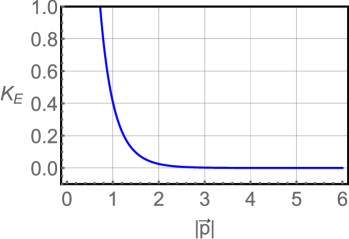
Figure 1: Plot of the function $K_{E}(x_{3},|\vec{p}|)$ of Eq. (IV.1) for $x_{3}=2$ and $M=2$ as a function of $|\vec{p}|$.

IV.2 Electron-positron annihilation at tree-level

Our intention is to check the perturbative validity of the optical theorem for the theory defined by Eq. (2). To do so, we have to couple the modified photon theory to standard Dirac fermions in $(2+1)$ dimensions, i.e., we will consider a modified QED in three dimensions (QED₃). A summary on a theory of Dirac spinors in $(2+1)$ dimensions is given in appendix D. We then write the total Lagrange density as

$$\mathcal{L}_{\mathrm{tot}} =\mathcal{L}+\mathcal{L}_{\psi,\upgamma}\,,$$ (90a)

$$\mathcal{L}_{\psi,\upgamma} =\overline{\psi}[\gamma^{\mu}(\mathrm{i}\partial_{\mu}-eA_{\mu})+m]\psi\,,$$ (90b)

with $\mathcal{L}$ given by Eq. (2). Here, $e$ is the electric charge, $m$ the fermion mass, $\psi$ is a four-component Dirac spinor, and $\gamma^{\mu}$ the set of three Dirac matrices of Eq. (D). Note again that Lorentz indices run over $0,1,2$.

The optical theorem establishes a connection between the forward-scattering amplitude of a particular particle physics process and the decay rates or total cross sections of processes that are obtained by cutting the Feynman diagram of the forward-scattering amplitude into two pieces. We will study processes at tree-level and one-loop order that involve the gauge-field propagator (10a) of the theory Bhabha1 ; Bhabha2 . Let us start with the polarized forward scattering annihilation process of electron-positron pairs, $\mathrm{e^{+}e^{-}}\to\mathrm{e^{+}e^{-}}$ of Fig. 2.

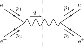
Figure 2: Polarized forward scattering electron-positron annihilation where a cut of the gauge field propagator is indicated by the dashed line. The three-momenta of the incoming particles are $p_{1}$, $p_{2}$ where the three-momentum of the intermediate modified photon is denoted as $q$.

The corresponding amplitude is given by

$$\mathrm{i}\mathcal{M}_{F} =\bar{v}(p_{2})(-\mathrm{i}e\gamma^{\mu})u(p_{1})\left(\mathrm{i}D^{F}_{\mu\nu}(\xi,q)\right)$$

$$\phantom{{}={}}\times\bar{u}(p_{1})(-\mathrm{i}e\gamma^{\nu})v(p_{2})\,,$$ (91)

with the Feynman propagator of Eq. (75) and $q=p_{1}+p_{2}$. Particle and antiparticle spinors of a particular spin projection are denoted as $u(p)$ and $v(p)$, respectively, and correspond to those of Eqs. (D), (D). Considering polarized scattering is not crucial for the verification of the optical theorem, though. It just simplifies the expressions, as the polarizations of the incoming and outgoing particles need not be averaged or summed over. Note also that we suppress the spin index for external spinors. Now, we can write

$$\mathcal{M}_{F}=-e^{2}\mathcal{M}^{\mu}(p_{1},p_{2})D^{F}_{\mu\nu}(\xi,q)\mathcal{M}^{{\dagger}\nu}(p_{1},p_{2})\,,$$ (92)

where

$$\mathcal{M}^{\mu}(p_{1},p_{2}) = \bar{v}(p_{2})\gamma^{\mu}u(p_{1})\,,$$ (93)

$$\mathcal{M}^{{\dagger}\nu}(p_{1},p_{2}) = \bar{u}(p_{1})\gamma^{\nu}v(p_{2})\,.$$ (94)

The process that results from cutting the diagram of the forward scattering amplitude into two pieces is the production of a modified photon by an electron positron pair. In contrast to what happens in standard QED, the cross section of this process is not necessarily equal to zero due to energy-momentum conservation. The reason is the presence of the massive ghost, which can render the process possible. In this case, the condition of energy conservation can be evaluated in the center-of-mass frame: $|\vec{p}_{1}|=|\vec{p}_{2}|=1/2g$. Therefore, it will be sufficient to prove unitarity by considering the contributions to the imaginary part (or discontinuity) of the amplitude for the massive ghost.

In the forward scattering amplitude of Eq. (92) an integral over the three-momentum $q$ of the intermediate state can be introduced that is canceled again by the three-dimensional $\delta$ function of total energy-momentum conservation (which is equivalent to energy-momentum conservation at each vertex):

$$\mathcal{M}_{F} =-e^{2}\int\frac{\mathrm{d}^{3}q}{(2\pi)^{3}}\mathcal{M}^{\mu}D^{F}_{\mu\nu}(\xi,q)\mathcal{M}^{{\dagger}\nu}$$

$$\phantom{{}={}}\times(2\pi)^{3}\delta^{(3)}(p_{1}+p_{2}-q)\,.$$ (95)

By inserting the Feynman propagator of Eq. (75), we have

$$\mathcal{M}_{F} =-e^{2}M^{2}\int\frac{\mathrm{d}^{3}q}{(2\pi)^{3}}\frac{\mathcal{M}^{\mu}G_{\mu\nu}(\xi,q)\mathcal{M}^{{\dagger}\nu}}{(q^{2}+\mathrm{i}\epsilon)(q^{2}-M^{2}+\mathrm{i}\epsilon)}$$

$$\phantom{{}={}}\times(2\pi)^{3}\delta^{(3)}(p_{1}+p_{2}-q)\,.$$ (96)

As the photon propagator is coupled to a conserved external current and energy-momentum is conserved at the vertex, we can use the Ward identity to get rid of all terms in the propagator proportional to this momentum: $q_{\mu}\mathcal{M}^{\mu}=0$. Doing so, allows for instating the tensor $T_{\mu\nu}$ of Eq. (51).

It is valuable to recall that

$$\frac{M^{2}}{(q^{2}+\mathrm{i}\epsilon)(q^{2}-M^{2}+\mathrm{i}\epsilon)}=-\frac{1}{q^{2}+\mathrm{i}\epsilon}+\frac{1}{q^{2}-M^{2}+\mathrm{i}\epsilon}\,.$$ (97)

By making use of the latter, we can decompose the denominator into two parts:

$$\mathcal{M}_{F} =e^{2}\int\frac{\mathrm{d}^{3}q}{(2\pi)^{3}}\left[\frac{\mathcal{M}^{\mu}T_{\mu\nu}(q)\mathcal{M}^{{\dagger}\nu}}{q^{2}+\mathrm{i}\epsilon}-\frac{\mathcal{M}^{\mu}T_{\mu\nu}(q)\mathcal{M}^{{\dagger}\nu}}{q^{2}-M^{2}+\mathrm{i}\epsilon}\right]$$

$$\phantom{{}={}}\times(2\pi)^{3}\delta^{(3)}(p_{1}+p_{2}-q)\,.$$ (98)

Now we insert the expression for $T_{\mu\nu}$ in terms of polarization vectors given in Eqs. (51a), (53) and obtain

$$\mathcal{M}_{F} =e^{2}\int\frac{\mathrm{d}^{3}q}{(2\pi)^{3}}\left[\frac{\sum_{\lambda,\lambda^{\prime}}\left(\mathcal{M}^{\mu}\bar{e}^{(\lambda)}_{\mu}\right)g_{\lambda\lambda^{\prime}}\left(\mathcal{M}^{{\dagger}\nu}\bar{e}^{(\lambda^{\prime})*}_{\nu}\right)}{q^{2}+\mathrm{i}\epsilon}\right.$$

$$\phantom{{}={}}\hskip 56.9055pt\left.+\frac{\left(\mathcal{M}^{\mu}\bar{\varepsilon}^{(+)}_{\mu}\right)\left(\mathcal{M}^{{\dagger}\nu}\bar{\varepsilon}^{(+)*}_{\nu}\right)}{q^{2}-M^{2}+\mathrm{i}\epsilon}\right]$$

$$\phantom{{}={}}\hskip 56.9055pt\times(2\pi)^{3}\delta^{(3)}(p_{1}+p_{2}-q)\,.$$ (99)

Since it is not possible to satisfy energy-momentum conservation and the dispersion relation for the photon at the same time, the first contribution is zero. We are then left with

$$\mathcal{M}_{F} =e^{2}\int\frac{\mathrm{d}^{3}q}{(2\pi)^{3}}\frac{|\mathcal{M}^{\mu}\bar{\varepsilon}^{(+)}_{\mu}(q)|^{2}}{(q_{0}+\Omega_{q}-\mathrm{i}\epsilon)(q_{0}-\Omega_{q}+\mathrm{i}\epsilon)}$$

$$\phantom{{}={}}\times(2\pi)^{3}\delta^{(3)}(p_{1}+p_{2}-q)\,.$$ (100)

We perform the integration over $q_{0}$ by defining the center-of mass energy $\sqrt{s}=p_{1}^{0}+p_{2}^{0}$ and exploit the property of the $\delta$ function. This leads to

$$\mathcal{M}_{F}(s) =e^{2}\int\frac{\mathrm{d}^{2}\vec{q}}{(2\pi)^{3}}\frac{|\mathcal{M}^{\mu}\bar{\varepsilon}^{(+)}_{\mu}(\Omega_{q},\vec{q})|^{2}}{(\sqrt{s}+\Omega_{q}-\mathrm{i}\epsilon)(\sqrt{s}-\Omega_{q}+\mathrm{i}\epsilon)}$$

$$\phantom{{}={}}\times(2\pi)^{3}\delta^{(2)}(\vec{p}_{1}+\vec{p}_{2}-\vec{q})\,.$$ (101)

The imaginary part of the amplitude can be evaluated based on the identity

$$\lim_{\epsilon\rightarrow 0^{+}}\frac{1}{x\pm\mathrm{i}\epsilon}=\mathcal{P}\left(\frac{1}{x}\right)\mp\mathrm{i}\pi\delta(x)\,,$$ (102)

where $\mathcal{P}$ denotes the principal value. We also consider

$$\frac{2\Omega_{q}}{(\sqrt{s}+\Omega_{q}-\mathrm{i}\epsilon)(\sqrt{s}-\Omega_{q}+\mathrm{i}\epsilon)}$$

$$=\frac{1}{\sqrt{s}-\Omega_{q}+\mathrm{i}\epsilon}-\frac{1}{\sqrt{s}+\Omega_{q}-\mathrm{i}\epsilon}\,.$$ (103)

The result is

$$\text{Im}(\mathcal{M}_{F}(s)) =-e^{2}\int\frac{\mathrm{d}^{2}\vec{q}}{(2\pi)^{3}}|\mathcal{M}^{\mu}\bar{\varepsilon}^{(+)}_{\mu}(\Omega_{q},\vec{q})|^{2}$$

$$\phantom{{}={}}\times(2\pi)^{3}\delta^{(2)}(\vec{p}_{1}+\vec{p}_{2}-\vec{q})$$

$$\phantom{{}={}}\times\frac{\pi}{2\Omega_{q}}\left[\delta(\sqrt{s}-\Omega_{p})+\delta(\sqrt{s}+\Omega_{q})\right]\,.$$ (104)

The second $\delta$ function in Eq. (IV.2) involves a non-zero contribution coming from the possibility of negative energies. This can be seen in the following way. From the definition of the Feynman propagator one has

$$D^{F}_{\mu\nu}(z_{0},\vec{z}) =\theta(z_{0})D^{(+)}_{\mu\nu}(z_{0},\vec{z})$$

$$\phantom{{}={}}+\theta(-z_{0})D^{(-)}_{\mu\nu}(z_{0},\vec{z})\,,$$ (105)

Performing a coordinate Poincaré transformation, for instance, a constant time translation that adds a constant purely timelike three-vector to $z$ such that $z_{0}\to-z_{0}$, one has

$$D^{F}_{\mu\nu}(-z_{0},\vec{z}) =\theta(-z_{0})D^{(+)}_{\mu\nu}(-z_{0},\vec{z})$$

$$\phantom{{}={}}+\theta(z_{0})D^{(-)}_{\mu\nu}(-z_{0},\vec{z})\,.$$ (106)

The interpretation is that negative energies occur in the opposite flow of time. This is precisely the reason why we include the second $\delta$ function in Eq. (IV.2). In the literature, the latter is sometimes represented by a cut with a shaded region indicating the corresponding direction of energy flow Perturbativeunitarity .

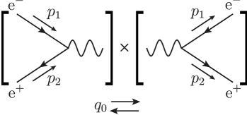
Figure 3: After cutting the photon propagator in the diagram of Fig. 2, the sum over intermediate states in both directions of the energy flow is considered.

Finally, we can write

$$2\text{Im}(\mathcal{M}_{F}(s)) =-e^{2}\int\frac{\mathrm{d}^{3}q}{(2\pi)^{3}}|\mathcal{M}^{\mu}\bar{\varepsilon}^{(+)}_{\mu}(q)|^{2}$$

$$\phantom{{}={}}\times(2\pi)^{3}\delta^{(3)}(p_{1}+p_{2}-q)(2\pi)\delta(q^{2}-M^{2})$$

$$\phantom{{}={}}\times\left[\theta(q_{0})+\theta(-q_{0})\right]\,,$$ (107)

which represents the sum of diagrams with energy flow in the positive and negative direction as represented in Fig. 3.

Now we come to the crucial point in the analysis where we must introduce some of the ideas developed by Lee and Wick. As a first observation, the negative global sign in Eq. (IV.2) may threaten unitarity since the left-hand side of the latter equation, which is related to the cross section, is positive-definite. To overcome this problem, we apply the Lee-Wick prescription that removes the negative-metric states from the asymptotic Hilbert space. Furthermore, as long as the energy of the incoming state is low enough, the argument of $\delta(q^{2}-M^{2})$ is impossibly different from zero due to the large mass of the ghost. The latter will simply not be excited under this condition. Then unitarity is guaranteed in a direct way just as in the standard case Lee-Wick:Negative ; Lee-Wick:Finite ; Anon-analytic .

IV.3 Compton scattering at one-loop level

Our next step is to study unitarity when virtual ghosts arise in loop diagrams. We analyze the optical theorem for the (polarized) Compton scattering process of Fig. 4. The forward-scattering amplitude at one-loop level for this process in the extended Maxwell-Chern-Simons theory in $(2+1)$ dimensions given by the Lagrangian (2) reads

$$\mathrm{i}\mathcal{M} =\epsilon^{(\lambda)\ast}_{\beta}(k)\bar{u}(p^{\prime})(-\mathrm{i}e\gamma^{\beta})\left(\frac{\mathrm{i}(\not{p}+m)}{p^{2}-m^{2}+\mathrm{i}\epsilon}\right)(-\mathrm{i}e\gamma^{\mu})\int\frac{\mathrm{d}^{3}q}{(2\pi)^{3}}\frac{\mathrm{i}(\not{p}-\not{q}+m)}{(p-q)^{2}-m^{2}+\mathrm{i}\epsilon}$$

$$\phantom{{}={}}\times(\mathrm{i}D^{F}_{\mu\nu}(q))(-\mathrm{i}e\gamma^{\nu})\left(\frac{\mathrm{i}(\not{p}+m)}{p^{2}-m^{2}+\mathrm{i}\epsilon}\right)(-\mathrm{i}e\gamma^{\alpha})u(p^{\prime})\epsilon^{(\lambda)}_{\alpha}(k)\,,$$ (108)

where the external electrons and photons are considered as polarized. The fermion propagator for $(2+1)$-dimensional Dirac theory of Eq. (D.12) has been inserted. For simplicity, we choose the particular gauge fixing parameter $\xi=1$ and employ the Feynman propagator of Eq. (74). We introduce the following short-hand notation for expressions formed from external spinors and polarization vectors:

$$J_{1}^{(\lambda)}(p^{\prime},k) =\epsilon^{\ast(\lambda)}_{\beta}(k)\bar{u}(p^{\prime})\gamma^{\beta}\,,$$ (109a)

$$J_{2}^{(\lambda)}(p^{\prime},k) =\gamma^{\alpha}u(p^{\prime})\epsilon^{(\lambda)}_{\alpha}(k)\,,$$ (109b)

and rewrite the denominators of Eq. (IV.3) in terms of the poles. We also work in the center-of-mass frame where $\vec{p}=\vec{0}$ and use Eq. (97) to obtain

$$\mathrm{i}\mathcal{M} =-e^{4}J_{1}^{(\lambda)}(p^{\prime},k)\left(\frac{\not{p}+m}{p^{2}-m^{2}+\mathrm{i}\epsilon}\right)\gamma^{\mu}\int\frac{\mathrm{d}^{3}q}{(2\pi)^{3}}\frac{\not{p}-\not{q}+m}{(q_{0}-p_{0}-E_{q}+\mathrm{i}\epsilon)(q_{0}-p_{0}+E_{q}-\mathrm{i}\epsilon)}$$

$$\phantom{{}={}}\times T_{\mu\nu}(q)\left[\frac{1}{(q_{0}-\omega_{q}+\mathrm{i}\epsilon)(q_{0}+\omega_{q}-\mathrm{i}\epsilon)}-\frac{1}{(q_{0}-\Omega_{q}+\mathrm{i}\epsilon)(q_{0}+\Omega_{q}-\mathrm{i}\epsilon)}\right]$$

$$\phantom{{}={}}\times\gamma^{\nu}\left(\frac{\not{p}+m}{p^{2}-m^{2}+\mathrm{i}\epsilon}\right)J_{2}^{(\lambda)}(p^{\prime},k)\,.$$ (110)

Let us decompose the amplitude into a sum of amplitudes via

$$\mathcal{M} = \mathcal{M}^{(1)}+\mathcal{M}^{(2)}\,,$$ (111a)

with

$$\mathrm{i}\mathcal{M}^{(1)} =-e^{4}J_{1}^{(\lambda)}(p^{\prime},k)\left(\frac{\not{p}+m}{p^{2}-m^{2}+\mathrm{i}\epsilon}\right)\gamma^{\mu}\int\frac{\mathrm{d}^{2}\vec{q}\,\mathrm{d}q_{0}}{(2\pi)^{3}}\frac{\not{p}-\not{q}+m}{(q_{0}-p_{0}-E_{q}+\mathrm{i}\epsilon)(q_{0}-p_{0}+E_{q}-\mathrm{i}\epsilon)}$$

$$\phantom{{}={}}\times\frac{T_{\mu\nu}(q)}{(q_{0}-\omega_{q}+\mathrm{i}\epsilon)(q_{0}+\omega_{q}-\mathrm{i}\epsilon)}\gamma^{\nu}\left(\frac{\not{p}+m}{p^{2}-m^{2}+\mathrm{i}\epsilon}\right)J_{2}^{(\lambda)}(p^{\prime},k)\,,$$ (111b)

and

$$\mathrm{i}\mathcal{M}^{(2)} =e^{4}J_{1}^{(\lambda)}(p^{\prime},k)\left(\frac{\not{p}+m}{p^{2}-m^{2}+\mathrm{i}\epsilon}\right)\gamma^{\mu}\int\frac{\mathrm{d}^{2}\vec{q}\,\mathrm{d}q_{0}}{(2\pi)^{3}}\frac{\not{p}-\not{q}+m}{(q_{0}-p_{0}-E_{q}+\mathrm{i}\epsilon)(q_{0}-p_{0}+E_{q}-\mathrm{i}\epsilon)}$$

$$\phantom{{}={}}\times\frac{T_{\mu\nu}(q)}{(q_{0}-\Omega_{q}+\mathrm{i}\epsilon)(q_{0}+\Omega_{q}-\mathrm{i}\epsilon)}\gamma^{\nu}\left(\frac{\not{p}+m}{p^{2}-m^{2}+\mathrm{i}\epsilon}\right)J_{2}^{(\lambda)}(p^{\prime},k)\,.$$ (111c)

Our next step is to integrate over the complex variable $q_{0}$ by using the residue theorem and closing the contour in the lower half plane of the complex $q_{0}$ plane. Each integrand has two contributing poles leading to four poles $q_{0}=z_{i}$ ($i=1\dots 4$), in total. For the first integrand we have

$$z_{1} =p_{0}+E_{q}-\mathrm{i}\epsilon\,,$$ (112a)

$$z_{2} =\omega_{q}-\mathrm{i}\epsilon\,,$$ (112b)

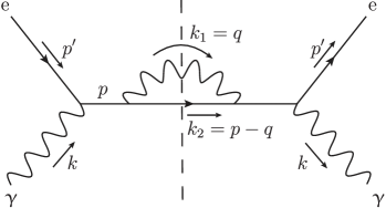
Figure 4: Forward Compton scattering with one-loop correction of the fermion propagator included. The cut of both propagators is indicated by a dashed line. The external three-momenta are given by $k$ and $p^{\prime}$.

where $E_{q}$ is the dispersion relation (D.13) of a massive fermion in $(2+1)$ dimensions. The poles of the second integrand are given by

$$z_{3} =p_{0}+E_{q}-\mathrm{i}\epsilon\,,$$ (113a)

$$z_{4} =\Omega_{q}-\mathrm{i}\epsilon\,.$$ (113b)

We then arrive at

$$\mathcal{M}^{(1)} =-e^{4}J_{1}^{(\lambda)}(p^{\prime},k)\left(\frac{\not{p}+m}{p^{2}-m^{2}}\right)\gamma^{\mu}$$

$$\phantom{{}={}}\times\int\frac{\mathrm{d}^{2}\vec{q}}{(2\pi)^{2}}(\not{p}-\not{q}+m)T_{\mu\nu}(q)$$

$$\phantom{{}={}}\times\left(\mathrm{Res}(z_{1})+\mathrm{Res}(z_{2})\right)\gamma^{\nu}\left(\frac{\not{p}+m}{p^{2}-m^{2}}\right)$$

$$\phantom{{}={}}\times J_{2}^{(\lambda)}(p^{\prime},k)\,,$$ (114)

and

$$\mathcal{M}^{(2)} =e^{4}J_{1}^{(\lambda)}(p^{\prime},k)\left(\frac{\not{p}+m}{p^{2}-m^{2}}\right)\gamma^{\mu}$$

$$\phantom{{}={}}\times\int\frac{\mathrm{d}^{2}\vec{q}}{(2\pi)^{2}}(\not{p}-\not{q}+m)T_{\mu\nu}(q)$$

$$\phantom{{}={}}\times\left(\mathrm{Res}(z_{3})+\mathrm{Res}(z_{4})\right)\gamma^{\nu}\left(\frac{\not{p}+m}{p^{2}-m^{2}}\right)$$

$$\phantom{{}={}}\times J_{2}^{(\lambda)}(p^{\prime},k)\,,$$ (115)

with the residues

$$\mathrm{Res}(z_{1}) =\frac{-1}{2E_{q}(p_{0}+E_{q}-\omega_{q})(p_{0}+E_{q}+\omega_{q}-\mathrm{i}\epsilon)}\,,$$ (116a)

$$\mathrm{Res}(z_{2}) =\frac{-1}{2\omega_{q}(p_{0}+E_{q}-\omega_{q})(p_{0}-E_{q}-\omega_{q}+\mathrm{i}\epsilon)}\,,$$ (116b)

and

$$\mathrm{Res}(z_{3}) =\frac{-1}{2E_{q}(p_{0}+E_{q}-\Omega_{q})(p_{0}+E_{q}+\Omega_{q}-\mathrm{i}\epsilon)}\,,$$ (117a)

$$\mathrm{Res}(z_{4}) =\frac{-1}{2\Omega_{q}(p_{0}+E_{q}-\omega_{q})(p_{0}-E_{q}-\Omega_{q}+\mathrm{i}\epsilon)}\,,$$ (117b)

where we have rescaled the parameter $\epsilon$ and set $\epsilon\to 0$ where it is not important.

Our amplitude $\mathcal{M}$ of Eq. (IV.3) considered as an analytic function of the complex variable $q_{0}$ has a branch cut along the real axis. In order to extract the imaginary part of the diagram we will compute the imaginary parts of the residues by using the identity (102). We obtain

$$\mathrm{Im}(\mathrm{Res}(z_{1})) =\frac{\pi\delta(p_{0}+\omega_{p}+E_{q})}{4\omega_{q}E_{q}}\,,$$ (118a)

$$\mathrm{Im}(\mathrm{Res}(z_{2})) =\frac{\pi\delta(p_{0}-\omega_{p}-E_{q})}{4\omega_{q}E_{q}}\,,$$ (118b)

$$\mathrm{Im}(\mathrm{Res}(z_{3})) =\frac{\pi\delta(p_{0}+\Omega_{p}+E_{q})}{4\Omega_{q}E_{q}}\,,$$ (118c)

$$\mathrm{Im}(\mathrm{Res}(z_{4})) =\frac{\pi\delta(p_{0}-\Omega_{p}-E_{q})}{4\Omega_{q}E_{q}}\,.$$ (118d)

We can then write the imaginary parts of the amplitudes as

$$\mathrm{Im}(\mathcal{M}^{(1)}) = -e^{4}J_{1}^{(\lambda)}(p^{\prime},k)\left(\frac{\not{p}+m}{p^{2}-m^{2}}\right)\gamma^{\mu}\int\frac{\mathrm{d}^{2}\vec{q}}{(2\pi)^{3}}(\not{p}-\not{q}+m)T_{\mu\nu}(q)$$

$$\times\frac{(2\pi)\pi}{4\omega_{q}E_{q}}\left[\delta(p_{0}-\omega_{p}-E_{q})+\delta(p_{0}+\omega_{p}+E_{q})\right]\gamma^{\nu}\left(\frac{\not{p}+m}{p^{2}-m^{2}}\right)J_{2}^{(\lambda)}(p^{\prime},k)\,,$$

and in the same way

$$\mathrm{Im}(\mathcal{M}^{(2)}) = e^{4}J_{1}^{(\lambda)}(p^{\prime},k)\left(\frac{\not{p}+m}{p^{2}-m^{2}}\right)\gamma^{\mu}\int\frac{\mathrm{d}^{2}\vec{q}}{(2\pi)^{3}}(\not{p}-\not{q}+m)T_{\mu\nu}(q)$$

$$\times\frac{(2\pi)\pi}{4\Omega_{q}E_{q}}\left[\delta(p_{0}-\Omega_{p}-E_{q})+\delta(p_{0}+\Omega_{p}+E_{q})\right]\gamma^{\nu}\left(\frac{\not{p}+m}{p^{2}-m^{2}}\right)J_{2}^{(\lambda)}(p^{\prime},k)\,.$$

Now, we define

$$q = k_{1}\,,$$ (121a)

$$p-q = k_{2}\,,$$ (121b)

and use energy conservation expressed by the $\delta$ functions $\delta(p_{0}\pm\Omega_{p}\pm E_{q})$ and $\delta(p_{0}\pm\omega_{p}\pm E_{q})$. Furthermore, we employ the relation

$$\int\frac{\mathrm{d}^{2}\vec{q}}{(2\pi)^{3}}=\int\frac{\mathrm{d}^{2}\vec{k}_{1}}{(2\pi)^{3}}\int\frac{\mathrm{d}^{2}\vec{k}_{2}}{(2\pi)^{3}}\,(2\pi)^{3}\delta^{(2)}(\vec{p}-\vec{k}_{1}-\vec{k}_{2})\,,$$ (122)

to write the integrals over the spatial momentum components as integrals over three-momenta:

$$2\mathrm{Im}(\mathcal{M}^{(1)}) =-e^{4}J_{1}^{(\lambda)}(p^{\prime},k)\left(\frac{\not{p}+m}{p^{2}-m^{2}}\right)\gamma^{\mu}\left\{\int\frac{\mathrm{d}^{3}k_{1}}{(2\pi)^{3}}\int\frac{\mathrm{d}^{3}k_{2}}{(2\pi)^{3}}\,(\not{k}_{2}+m)\right.T_{\mu\nu}(k_{1})\left[\frac{2\pi\delta(k_{1}^{0}-\omega_{k_{1}})2\pi\delta(k_{2}^{0}-E_{k_{2}})}{(2\omega_{k_{1}})(2E_{k_{2}})}\right.$$

$$\phantom{{}={}}\hskip 28.45274pt\left.\left.+\frac{2\pi\delta(k_{1}^{0}+\omega_{k_{1}})2\pi\delta(k_{2}^{0}+E_{k_{2}})}{(2\omega_{k_{1}})(2E_{k_{2}})}\right](2\pi)^{3}\delta^{(3)}(p-k_{1}-k_{2})\right\}\gamma^{\nu}\left(\frac{\not{p}+m}{p^{2}-m^{2}}\right)J_{2}^{(\lambda)}(p^{\prime},k)\,,$$ (123)

and

$$2\mathrm{Im}(\mathcal{M}^{(2)}) =e^{4}J_{1}^{(\lambda)}(p^{\prime},k)\left(\frac{\not{p}+m}{p^{2}-m^{2}}\right)\gamma^{\mu}\left\{\int\frac{\mathrm{d}^{3}k_{1}}{(2\pi)^{3}}\int\frac{\mathrm{d}^{3}k_{2}}{(2\pi)^{3}}\,(\not{k}_{2}+m)\right.T_{\mu\nu}(k_{1})\left[\frac{2\pi\delta(k_{1}^{0}-\Omega_{k_{1}})2\pi\delta(k_{2}^{0}-E_{k_{2}})}{(2\Omega_{k_{1}})(2E_{k_{2}})}\right.$$

$$\phantom{{}={}}\hskip 28.45274pt\left.\left.+\frac{2\pi\delta(k_{1}^{0}+\Omega_{k_{1}})2\pi\delta(k_{2}^{0}+E_{k_{2}})}{(2\Omega_{k_{1}})(2E_{k_{2}})}\right](2\pi)^{3}\delta^{(3)}(p-k_{1}-k_{2})\right\}\gamma^{\nu}\left(\frac{\not{p}+m}{p^{2}-m^{2}}\right)J_{2}^{(\lambda)}(p^{\prime},k)\,.$$ (124)

Recall the relations (51a), (53) for the gauge polarization vectors. Furthermore, we apply the completeness relation (D.17a) for standard particle spinors in $(2+1)$ dimensions to this particular case, i.e.,

$$\sum_{s}u^{(s)}(k_{2})\bar{u}^{(s)}(k_{2})=\not{k}_{2}+m\,,$$ (125)

where the sum runs over the spin projection $s$ of the fermion in the former loop. Note that this spinor index is kept explicitly. We can then write

$$2\mathrm{Im}(\mathcal{M}^{(1)}) =-\sum_{s,\lambda^{\prime},\lambda^{\prime\prime}}\int\frac{\mathrm{d}^{3}k_{1}}{(2\pi)^{3}}\int\frac{\mathrm{d}^{3}k_{2}}{(2\pi)^{3}}\bigg{\{}-\mathrm{i}e^{2}J_{1}^{(\lambda)}(p^{\prime},k)\left(\frac{\not{p}+m}{p^{2}-m^{2}}\right)\gamma^{\mu}u^{(s)}(k_{2})\bar{e}_{\mu}^{(\lambda^{\prime})}(k_{1})\bigg{\}}$$

$$\phantom{{}={}}\times g_{\lambda^{\prime}\lambda^{\prime\prime}}\bigg{\{}\mathrm{i}e^{2}\bar{e}_{\nu}^{(\lambda^{\prime\prime})*}(k_{1})\bar{u}^{(s)}(k_{2})\gamma^{\nu}\left(\frac{\not{p}+m}{p^{2}-m^{2}}\right)J_{2}^{(\lambda)}(p^{\prime},k)\bigg{\}}2\pi\delta(k^{2}_{1})2\pi\delta(k_{2}^{2}-m^{2})(2\pi)^{3}\delta^{(3)}(p-k_{1}-k_{2})$$

$$\phantom{{}={}}\times\left[\theta(k_{1}^{0})\theta(k_{2}^{0})+\theta(-k_{1}^{0})\theta(-k_{2}^{0})\right]\,,$$ (126)

and

$$2\mathrm{Im}(\mathcal{M}^{(2)}) =\sum_{s}\int\frac{\mathrm{d}^{3}k_{1}}{(2\pi)^{3}}\int\frac{\mathrm{d}^{3}k_{2}}{(2\pi)^{3}}\bigg{\{}\mathrm{i}e^{2}J_{1}^{(\lambda)}(p^{\prime},k)\left(\frac{\not{p}+m}{p^{2}-m^{2}}\right)\gamma^{\mu}u^{(s)}(k_{2})\bar{\varepsilon}_{\mu}^{(+)}(k_{1})\bigg{\}}$$

$$\phantom{{}={}}\times\bigg{\{}\mathrm{i}e^{2}\bar{\varepsilon}_{\nu}^{(-)}(k_{1})\bar{u}^{(s)}(k_{2})\gamma^{\nu}\left(\frac{\not{p}+m}{p^{2}-m^{2}}\right)J_{2}^{(\lambda)}(p^{\prime},k)\bigg{\}}2\pi\delta(k^{2}_{1}-M^{2})2\pi\delta(k_{2}^{2}-m^{2})(2\pi)^{3}\delta^{(3)}(p-k_{1}-k_{2})$$

$$\phantom{{}={}}\times\left[\theta(k_{1}^{0})\theta(k_{2}^{0})+\theta(-k_{1}^{0})\theta(-k_{2}^{0})\right]\,.$$ (127)

In this way we obtain

$$2\mathrm{Im}(\mathcal{M}^{(1)}) =-\sum_{s,\lambda^{\prime},\lambda^{\prime\prime}}\int\frac{\mathrm{d}^{3}k_{1}}{(2\pi)^{3}}\int\frac{\mathrm{d}^{3}k_{2}}{(2\pi)^{3}}\bigg{\{}-\mathrm{i}e^{2}J_{1}^{(\lambda)}(p^{\prime},k)\left(\frac{\not{p}+m}{p^{2}-m^{2}}\right)J_{2}^{(\lambda^{\prime})}(k_{2},k_{1})\bigg{\}}$$

$$\phantom{{}={}}\times g_{\lambda^{\prime}\lambda^{\prime\prime}}\bigg{\{}\mathrm{i}e^{2}J_{1}^{(\lambda^{\prime\prime})}(k_{2},k_{1})\left(\frac{\not{p}+m}{p^{2}-m^{2}}\right)J_{2}^{(\lambda)}(p^{\prime},k)\bigg{\}}2\pi\delta(k^{2}_{1}-M^{2})2\pi\delta(k_{2}^{2}-m^{2})(2\pi)^{3}\delta^{(3)}(p-k_{1}-k_{2})$$

$$\phantom{{}={}}\times\left[\theta(k_{1}^{0})\theta(k_{2}^{0})+\theta(-k_{1}^{0})\theta(-k_{2}^{0})\right]\,,$$ (128)

and

$$2\mathrm{Im}(\mathcal{M}^{(2)}) =\sum_{s}\int\frac{\mathrm{d}^{3}k_{1}}{(2\pi)^{3}}\int\frac{\mathrm{d}^{3}k_{2}}{(2\pi)^{3}}\bigg{\{}\mathrm{i}e^{2}J_{1}^{(\lambda)}(p^{\prime},k)\left(\frac{\not{p}+m}{p^{2}-m^{2}}\right)J_{2}^{(+)}(k_{2},k_{1})\bigg{\}}$$

$$\phantom{{}={}}\times\bigg{\{}\mathrm{i}e^{2}J_{1}^{(-)}(k_{2},k_{1})\left(\frac{\not{p}+m}{p^{2}-m^{2}}\right)J_{2}^{(\lambda)}(p^{\prime},k)\bigg{\}}2\pi\delta(k^{2}_{1}-M^{2})2\pi\delta(k_{2}^{2}-m^{2})(2\pi)^{3}\delta^{(3)}(p-k_{1}-k_{2})$$

$$\phantom{{}={}}\times\left[\theta(k_{1}^{0})\theta(k_{2}^{0})+\theta(-k_{1}^{0})\theta(-k_{2}^{0})\right]\,,$$ (129)

where

$$J_{2}^{(+)}(k_{2},k_{1}) =\gamma^{\mu}u^{(s)}(k_{2})\bar{\varepsilon}_{\mu}^{(+)}(k_{1})\,,$$ (130a)

$$J_{1}^{(-)}(k_{2},k_{1}) =\bar{\varepsilon}_{\nu}^{(-)}(k_{1})\bar{u}^{(s)}(k_{2})\gamma^{\nu}\,.$$ (130b)

Let us define

$$g_{\lambda^{\prime}\lambda^{\prime\prime}}\mathcal{M}_{1}^{(\lambda^{\prime})}\mathcal{M}_{1}^{(\lambda^{\prime\prime}){\dagger}}=g_{\lambda^{\prime}\lambda^{\prime\prime}}\left(e^{2}J_{1}^{(\lambda)}(p^{\prime},k)\left(\frac{\not{p}+m}{p^{2}-m^{2}}\right)J_{2}^{(\lambda^{\prime})}(k_{2},k_{1})\right)\left(e^{2}J_{1}^{(\lambda^{\prime\prime})}(k_{2},k_{1})\left(\frac{\not{p}+m}{p^{2}-m^{2}}\right)J_{2}^{(\lambda)}(p^{\prime},k)\right)\,,$$ (131)

and

$${\mathcal{M}^{(+)}_{2}}{\mathcal{M}_{2}^{(-){\dagger}}}=\left(e^{2}J_{1}^{(\lambda)}(p^{\prime},k)\left(\frac{\not{p}+m}{p^{2}-m^{2}}\right)J_{2}^{(+)}(k_{2},k_{1})\right)\left(e^{2}J_{1}^{(-)}(k_{2},k_{1})\left(\frac{\not{p}+m}{p^{2}-m^{2}}\right)J_{2}^{(\lambda)}(p^{\prime},k)\right)\,.$$ (132)

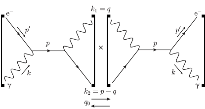
Figure 5: Sum over intermediate states and energy flow in the cut Compton diagram of Fig. 4.

Thus, we can express both imaginary parts as

$$2\mathrm{Im}(\mathcal{M}^{(1)}) =-\sum_{s,\lambda^{\prime},\lambda^{\prime\prime}}\int\frac{\mathrm{d}^{3}k_{1}}{(2\pi)^{3}}\int\frac{\mathrm{d}^{3}k_{2}}{(2\pi)^{3}}g_{\lambda^{\prime}\lambda^{\prime\prime}}\mathcal{M}_{1}^{(\lambda^{\prime})}\mathcal{M}_{1}^{(\lambda^{\prime\prime}){\dagger}}2\pi\delta(k^{2}_{1})2\pi\delta(k_{2}^{2}-m^{2})$$

$$\phantom{{}={}}\times(2\pi)^{3}\delta^{(3)}(p-k_{1}-k_{2})\left[\theta(k_{1}^{0})\theta(k_{2}^{0})+\theta(-k_{1}^{0})\theta(-k_{2}^{0})\right]\,,$$ (133)

and

$$2\mathrm{Im}(\mathcal{M}^{(2)}) =-\sum_{s}\int\frac{\mathrm{d}^{3}k_{1}}{(2\pi)^{3}}\int\frac{\mathrm{d}^{3}k_{2}}{(2\pi)^{3}}{\mathcal{M}^{(+)}_{2}}{\mathcal{M}_{2}^{(-){\dagger}}}2\pi\delta(k^{2}_{1}-M^{2})2\pi\delta(k_{2}^{2}-m^{2})$$

$$\phantom{{}={}}\times(2\pi)^{3}\delta^{(3)}(p-k_{1}-k_{2})\left[\theta(k_{1}^{0})\theta(k_{2}^{0})+\theta(-k_{1}^{0})\theta(-k_{2}^{0})\right]\,.$$ (134)

The sum in Eq. (IV.3) runs over the spin projection of the fermion and the polarization of the photon. Both particles were put on-shell by cutting the diagram of the forward-scattering amplitude (see Fig. 5) into two pieces. Note that the right-hand side of Eq. (IV.3) is zero, as the $\delta$ function does not provide a contribution due to the large mass scale $M$. This behavior is precisely the effect of the Lee-Wick prescription according to which the negative-norm states are removed from the asymptotic Hilbert space just as in the tree-level analysis (see Eq. (IV.2) and the subsequent paragraph). So, we conclude that the optical theorem and, therefore, unitarity continue being valid at one-loop order, as well.

V Conclusions and outlook

In this paper, we considered a higher-derivative Chern-Simons-type modification of electrodynamics in $(2+1)$ dimensions. We decomposed the Lagrangian of the model into a physical and a ghost sector and obtained the polarization vectors for the corresponding modes. In addition, the propagator of the theory was computed and it was demonstrated how it can be expressed in terms of the polarization vectors. Based on these findings, we performed the canonical quantization of the theory and studied its perturbative unitarity at both tree-level and one-loop order by checking the validity of the optical theorem.

Throughout this paper, we explicitly demonstrated that reflection positivity, known as a sufficient condition for unitarity, is satisfied. As the latter requirement applies to a free field theory only, we were interested in understanding unitarity when taking interactions into account. Hence, we coupled our theory to standard Dirac fermions in $(2+1)$ spacetime dimensions and evaluated the optical theorem for particular scattering processes. This analysis of unitarity revealed inconsistencies due to negative contributions at the pole of the ghost, as one should expect. However, by using the Lee-Wick prescription we have demonstrated that unitarity is conserved at both tree-level and one-loop order. The method of removing contributions from ghosts from the in- and out-states clearly provides this result. We applied the usual cutting rules of Feynman diagrams and amplitudes to guarantee the validity of the optical theorem. It was necessary to assume that the ghost mass is high enough, perhaps of the order of the Planck mass. It is expected that the situation at higher order in perturbation theory will not be very different.

It is also reasonable to expect that these results can be generalized naturally to the four-dimensional case where the higher-derivative Chern-Simons-like term breaks Lorentz symmetry. Some preliminary studies of unitarity in this alternative theory have been carried out in Bhabha1 . They are complemented by the analysis performed in our latest work Ferreira:2020wde .

Moreover, our opinion is that the results obtained here could serve as a base to explicitly define classes of higher-derivative theories consistent with the requirement of unitarity. In particular, our methodology could be useful for studies of various higher-derivative extensions of gravity including the Lorentz-breaking ones. We hope that this methodology will help to solve the problem of formulating a perturbatively consistent gravity model.

Appendix A Dirac formalism

We follow the Dirac procedure to reduce second-class constraints from the higher-derivative theory based on the Lagrangian (2) to zero testing and to find the Dirac brackets. From Eqs. (41a) and (41b), we have four primary second-class constraints

$$\chi_{0}(t,\vec{x}) = \Pi^{0}(t,\vec{x})-\frac{g}{2}\epsilon^{ij}\partial_{i}A_{j}(t,\vec{x})\,,$$ (A.1a)

$$\chi_{1}(t,\vec{x}) = P_{0}(t,\vec{x})+\dot{A}_{0}(t,\vec{x})+\frac{g}{2}\epsilon^{ij}\partial_{i}\dot{A}_{j}(t,\vec{x})\,,$$ (A.1b)

$$\varphi^{i}(t,\vec{x}) = \Pi^{i}(t,\vec{x})+\frac{g}{2}\epsilon^{ij}\dot{A}_{j}(t,\vec{x})-\frac{g}{2}\epsilon^{ij}\partial_{j}A_{0}(t,\vec{x})\,.$$

The non-vanishing elements of the algebra are

$$\left\{\chi_{1}(t,\vec{x}),\chi_{0}(t,\vec{y})\right\} = \delta^{(2)}(\vec{x}-\vec{y})\,,$$ (A.2a)

$$\left\{\varphi^{i}(t,\vec{x}),\chi_{1}(t,\vec{y})\right\} = -g\epsilon^{ij}\partial_{j}\,\delta^{(2)}(\vec{x}-\vec{y})\,,$$ (A.2b)

$$\left\{\varphi^{i}(t,\vec{x}),\varphi^{j}(t,\vec{y})\right\} = g\epsilon^{ij}\delta^{(2)}(\vec{x}-\vec{y})\,.$$ (A.2c)

The convention we use is that the derivatives act on the first set of spatial variables named $\vec{x}$, in general. To begin, let us introduce the notation $\varphi_{A}=(\chi_{0},\chi_{1},\varphi^{i})$, with $A=\bar{0},\bar{1},1,2$ and $i=1,2$. The matrix of the second-class constraints will be denoted by

$$C_{AB}(t;{\vec{x}},{\vec{y}})=\{\varphi_{A}(t,{\vec{x}}),\varphi_{B}(t,{\vec{y}})\}\,.$$ (A.3)

From Eq. (A.2c) we have

$$C_{AB}=\left[\begin{array}[]{cccc}0&-1&0&0\\ 1&0&-g\partial_{2}&g\partial_{1}\\ 0&-g\partial_{2}&0&g\\ 0&g\partial_{1}&-g&0\end{array}\right]\delta^{(2)}(\vec{x}-\vec{y})\,.$$ (A.4)

The inverse matrix is (where the $\delta$ function is not inverted):

$$C_{AB}^{-1}=\left[\begin{array}[]{cccc}0&1&-\partial_{1}&-\partial_{2}\\ -1&0&0&0\\ -\partial_{1}&0&0&-1/g\\ -\partial_{2}&0&1/g&0\end{array}\right]\delta^{(2)}(\vec{x}-\vec{y})\,.$$ (A.5)

The nonzero components are

$$C_{\bar{0}\bar{1}}^{-1}(\vec{x},\vec{y}) =-C_{\bar{1}\bar{0}}^{-1}(\vec{x},\vec{y})=\delta^{(2)}(\vec{x}-\vec{y})\,,$$ (A.6a)

$$C_{\bar{0}i}^{-1}(\vec{x},\vec{y}) =C_{i\bar{0}}^{-1}(\vec{x},\vec{y})=-\partial_{i}\delta^{(2)}(\vec{x}-\vec{y})\,,$$ (A.6b)

$$C_{ij}^{-1}(\vec{x},\vec{y}) =-\frac{1}{g}\,\epsilon^{ij}\delta^{(2)}(\vec{x}-\vec{y}),\qquad i,j=1,2\,.$$ (A.6c)

The Dirac brackets are defined by

$$\{X,Y\}^{*}=\{X,Y\}-\{X,\varphi_{A}\}\;C^{-1}_{AB}\;\{\varphi_{B},Y\}\,.$$ (A.7)

We promote the Dirac algebra to the equal-time commutators satisfied by the fields and obtain

$$\left[A_{0}(t,\vec{x}),\dot{A}_{0}(t,\vec{y})\right] =-\mathrm{i}\delta^{(2)}(\vec{x}-\vec{y})\,,$$ (A.8a)

$$\left[A_{0}({t,\vec{x}}),P_{0}({t,\vec{y}})\right] =\mathrm{i}\delta^{(2)}(\vec{x}-\vec{y})\,,$$ (A.8b)

$$\left[A_{0}({t,\vec{x}}),P^{i}(t,{\vec{y}})\right] =\frac{\mathrm{i}g}{2}\epsilon^{ij}\partial_{j}\,\delta^{(2)}(\vec{x}-\vec{y})\,,$$ (A.8c)

$$\left[\dot{A}_{i}({t,\vec{x}}),\dot{A}_{j}(t,{\vec{y}})\right] =-\frac{\mathrm{i}}{g}\epsilon^{ij}\delta^{(2)}(\vec{x}-\vec{y})\,,$$ (A.8d)

$$\left[\dot{A}_{i}({t,\vec{x}}),\dot{A}_{0}(t,{\vec{y}})\right] =-\mathrm{i}\partial_{i}\,\delta^{(2)}(\vec{x}-\vec{y})\,,$$ (A.8e)

$$\left[\dot{A}_{i}({t,\vec{x}}),P_{0}(t,{\vec{y}})\right] =\frac{\mathrm{i}}{2}\partial_{i}\,\delta^{(2)}(\vec{x}-\vec{y})\,,$$ (A.8f)

$$\left[\dot{A}_{i}({t,\vec{x}}),P^{j}(t,{\vec{y}})\right] =\frac{\mathrm{i}g}{2}\epsilon^{jk}\partial_{i}\partial_{k}\delta^{(2)}(\vec{x}-\vec{y})\,,$$ (A.8g)

$$\left[\dot{A}_{i}({t,\vec{x}}),\Pi^{j}(t,{\vec{y}})\right] =\frac{\mathrm{i}}{2}\delta_{ij}\,\delta^{(2)}(\vec{x}-\vec{y})\,,$$ (A.8h)

$$\left[P_{0}({t,\vec{x}}),\Pi^{i}(t,{\vec{y}})\right] =\frac{\mathrm{i}g}{4}\epsilon^{ij}\partial_{j}\,\delta^{(2)}(\vec{x}-\vec{y})\,,$$ (A.8i)

$$\left[\Pi_{0}({t,\vec{x}}),P^{i}(t,{\vec{y}})\right] =-\frac{\mathrm{i}g}{2}\epsilon^{ij}\partial_{j}\,\delta^{(2)}(\vec{x}-\vec{y})\,,$$ (A.8j)

$$\left[\Pi^{i}({t,\vec{x}}),\Pi^{j}(t,{\vec{y}})\right] =-\frac{\mathrm{i}g}{4}\epsilon^{ij}\delta^{(2)}(\vec{x}-\vec{y})\,.$$ (A.8k)

Note that the momentum $P^{\mu}$ has been changed in comparison to that employed in Ref. testing and, consequently, we have obtained a different algebra.

Appendix B The Hamiltonian

The current section delivers a detailed demonstration on how the Hamiltonian of the theory given by Eq. (2) can be expressed in terms of creation and annihilation operators. We consider the Hamiltonian (42) written as

$$H=H_{\bar{A}}+H_{G}\,,$$ (B.1)

where by using the decomposition (45) we have

$$H_{\bar{A}} = \int\mathrm{d}^{2}x\left(-\frac{1}{2}\dot{\bar{A}}_{\mu}(\hat{U}^{\mu\nu})\dot{\bar{A}}_{\nu}+\frac{1}{2}\bar{A}_{\mu}(\hat{U}^{\mu\nu})\nabla^{2}\bar{A}_{\nu}\right)\,,$$

$$H_{G} = \frac{g}{2}\int\mathrm{d}^{2}x\,\epsilon^{ij}\dot{G}_{i}\Box G_{j}\,.$$ (B.3)

Above, we have applied the equation of motion (46) for the ghost and $\Box\bar{A}_{\mu}=0$ for the photon.

Let us define

$$H^{\text{kin}}_{\bar{A}} = -\frac{1}{2}\int\mathrm{d}^{2}x\,\dot{\bar{A}}_{\mu}\hat{U}^{\mu\nu}\dot{\bar{A}}_{\nu}\,,$$ (B.4)

$$H^{\text{pot}}_{\bar{A}} = \frac{1}{2}\int\mathrm{d}^{2}x\,\bar{A}_{\mu}\hat{U}^{\mu\nu}\nabla^{2}\bar{A}_{\nu}\,.$$ (B.5)

Inserting the photon field operator of Eq. (III.1), the first contribution reads

$$H^{\text{kin}}_{\bar{A}} =\frac{1}{8}\int\frac{\mathrm{d}^{2}\vec{p}}{(2\pi)^{2}}\sum_{\lambda,\lambda^{\prime}}\left[a^{(\lambda)}_{\vec{p}}a^{(\lambda^{\prime})}_{-\vec{p}}\bar{e}^{(\lambda)}_{\mu}(\vec{p})U^{\mu\nu}_{-\vec{p}}\,\bar{e}^{(\lambda^{\prime})}_{\nu}(-\vec{p})e^{-2\mathrm{i}\omega_{\vec{p}}x_{0}}-a^{(\lambda)}_{\vec{p}}a^{(\lambda^{\prime}){\dagger}}_{\vec{p}}\bar{e}^{(\lambda)}_{\mu}(\vec{p})U^{\mu\nu*}_{\vec{p}}\bar{e}^{(\lambda^{\prime})*}_{\nu}(\vec{p})\right.$$

$$\phantom{{}={}}\hskip 68.28644pt\left.-\,a^{(\lambda){\dagger}}_{\vec{p}}a^{(\lambda^{\prime})}_{\vec{p}}\bar{e}^{(\lambda)*}_{\mu}(\vec{p})U^{\mu\nu}_{\vec{p}}\bar{e}^{(\lambda^{\prime})}_{\nu}(\vec{p})+a^{(\lambda){\dagger}}_{\vec{p}}a^{(\lambda^{\prime}){\dagger}}_{-\vec{p}}\bar{e}^{(\lambda)*}_{\mu}(\vec{p})U^{\mu\nu*}_{-\vec{p}}\,\bar{e}^{(\lambda^{\prime})*}_{\nu}(-\vec{p})e^{2\mathrm{i}\omega_{\vec{p}}x_{0}}\right]\,,$$ (B.6)

where $U^{\mu\nu}_{\vec{p}}=(\eta^{\mu\nu}-\mathrm{i}g\epsilon^{\mu\beta\nu}p_{\beta})_{p_{0}=\omega_{p}}$ corresponds to Eq. (42b) in momentum space.

In the same way,

$$H^{\text{pot}}_{\bar{A}} =-\frac{1}{8}\int\frac{\mathrm{d}^{2}\vec{p}}{(2\pi)^{2}}\sum_{\lambda,\lambda^{\prime}}\frac{\vec{p}^{\,2}}{\omega_{\vec{p}}^{2}}\left[a^{(\lambda)}_{\vec{p}}a^{(\lambda^{\prime})}_{-\vec{p}}\bar{e}^{(\lambda)}_{\mu}(\vec{p})U^{\mu\nu}_{-\vec{p}}\,\bar{e}^{(\lambda^{\prime})}_{\nu}(-\vec{p})e^{-2\mathrm{i}\omega_{\vec{p}}x_{0}}+a^{(\lambda)}_{\vec{p}}a^{(\lambda^{\prime}){\dagger}}_{\vec{p}}\bar{e}^{(\lambda)}_{\mu}(\vec{p})U^{\mu\nu*}_{\vec{p}}\bar{e}^{(\lambda^{\prime})*}_{\nu}(\vec{p})\right.$$

$$\phantom{{}={}}\hskip 91.04872pt\left.+\,a^{(\lambda){\dagger}}_{\vec{p}}a^{(\lambda^{\prime})}_{\vec{p}}\bar{e}^{(\lambda)*}_{\mu}(\vec{p})U^{\mu\nu}_{\vec{p}}\bar{e}^{(\lambda^{\prime})}_{\nu}(\vec{p})+a^{(\lambda){\dagger}}_{\vec{p}}a^{(\lambda^{\prime}){\dagger}}_{-\vec{p}}\bar{e}^{(\lambda)*}_{\mu}(\vec{p})U^{\mu\nu*}_{-\vec{p}}\,\bar{e}^{(\lambda^{\prime})*}_{\nu}(-\vec{p})e^{2\mathrm{i}\omega_{\vec{p}}x_{0}}\right]\,,$$ (B.7)

We see that the first and last terms vanish due to the global factor $1-\vec{p}^{\,2}/\omega_{p}^{2}$, while the other terms pick up a factor of $1+\vec{p}^{\,2}/\omega_{p}^{2}=2$. We arrive at

$$H_{\bar{A}}=-\frac{1}{4}\int\frac{\mathrm{d}^{2}\vec{p}}{(2\pi)^{2}}\sum_{\lambda,\lambda^{\prime}}\eta_{\lambda\lambda^{\prime}}\Big{(}a^{(\lambda)}_{\vec{p}}a^{(\lambda^{\prime}){\dagger}}_{\vec{p}}+a^{(\lambda){\dagger}}_{\vec{p}}a^{(\lambda^{\prime})}_{\vec{p}}\Big{)}\,,$$

where we have used

$$\bar{e}^{(\lambda)}_{\mu}U^{\mu\nu*}_{\vec{p}}\bar{e}^{*(\lambda^{\prime})}_{\nu}=g^{\lambda\lambda^{\prime}}\,.$$ (B.9)

and its complex conjugated.

For the ghost part we insert the ghost field operator of Eq. (III.1) and obtain

$$H_{G} =\frac{g}{8}\int\frac{\mathrm{d}^{2}\vec{p}}{(2\pi)^{2}}\frac{\mathrm{i}\epsilon^{ij}}{g^{2}\Omega_{p}}\left[b_{\vec{p}}\,b^{{\dagger}}_{\vec{p}}\,\bar{\varepsilon}_{i}^{(+)}(\vec{p})\,\bar{\varepsilon}_{j}^{(+)*}(\vec{p})\right.$$

$$\phantom{{}={}}\hskip 56.9055pt\left.-b^{{\dagger}}_{\vec{p}}\,b_{\vec{p}}\,\bar{\varepsilon}_{i}^{(+)*}(\vec{p})\,\bar{\varepsilon}_{j}^{(+)}(\vec{p})\right]\,,$$ (B.10)

where we have used that $p^{2}=1/g^{2}$ as well as

$$\epsilon^{ij}\bar{\varepsilon}_{i}^{(+)}(\vec{p})\bar{\varepsilon}_{j}^{(+)}(-\vec{p})=0\,,$$ (B.11a)

since

$$\bar{\varepsilon}_{k}^{(+)}(-\vec{p})=-\bar{\varepsilon}_{k}^{(+)}(\vec{p})\,,$$ (B.11b)

for $k=1,2$. We then arrive at

$$H_{G} = -\frac{1}{4}\int\frac{\mathrm{d}^{2}\vec{p}}{(2\pi)^{2}}\left(b_{\vec{p}}\,b^{{\dagger}}_{\vec{p}}+b^{{\dagger}}_{\vec{p}}\,b_{\vec{p}}\right)\,,$$ (B.12)

where we have also employed

$$\epsilon^{ij}\bar{\varepsilon}_{i}^{(\pm)}\bar{\varepsilon}_{j}^{(\pm)\ast}|_{p_{0}=\Omega_{p}}=\pm 2\mathrm{i}g\Omega_{p}\,.$$ (B.13)

This proves our expression (III.1).

Appendix C Extended equal-time commutators

In this section we intend to compute the equal-time commutators for the field operators that emerge from field theory of higher derivatives defined by Eq. (2). Consider the basic commutator

$$\left[A_{\mu}(x),A_{\nu}(y)\right]=\left[\bar{A}_{\mu}(x),\bar{A}_{\nu}(y)\right]+\left[G_{\mu}(x),G_{\nu}(y)\right]\,.$$ (C.1a)

with

$$\left[\bar{A}_{\mu}(x),\bar{A}_{\nu}(y)\right] =-\int\frac{\mathrm{d}^{2}\vec{p}}{(2\pi)^{2}}\frac{1}{2\omega_{p}}\left(T_{\mu\nu}(p)e^{-\mathrm{i}p\cdot(x-y)}\right.$$

$$\phantom{{}={}}\left.-T_{\nu\mu}(p)e^{\mathrm{i}p\cdot(x-y)}\right)_{p_{0}=\omega_{p}}\,,$$ (C.1b)

$$\left[G_{\mu}(x),G_{\nu}(y)\right] =\int\frac{\mathrm{d}^{2}\vec{p}}{(2\pi)^{2}}\frac{1}{2\Omega_{p}}\left(T_{\mu\nu}(p)e^{-\mathrm{i}p\cdot(x-y)}\right.$$

$$\phantom{{}={}}\left.-T_{\nu\mu}(p)e^{\mathrm{i}p\cdot(x-y)}\right)_{p_{0}=\Omega_{p}}\,.$$ (C.1c)

To derive the Dirac commutators we work directly with the field operators of Eqs. (III.1) and (III.1). Our strategy will be as follows:

• We consider the basic commutator (C.1a) and construct the various elements in phase space by applying the different operators on the fields.

• For a commutator containing $\Box A_{\mu}(t,{\vec{x}})$ we use the identities $\Box\bar{A}_{\mu}(t,{\vec{x}})=0$ and $\Box G_{\mu}(t,{\vec{x}})=-\frac{1}{g^{2}}G_{\mu}(t,{\vec{x}})$.

• Whenever an integral involves momentum variables we use the relation $p_{\mu}=\mathrm{i}\partial_{\mu}$, whereupon derivatives can be extracted from the integral.

• To treat derivatives for the second variable $\partial_{i}^{y}$, we integrate by parts to produce $\partial_{i}^{x}$ whereby an additional minus sign occurs.

• We assume that the spatial derivatives $\partial_{i}$ act on the first variable $\vec{x}$ of $\delta$ functions in all final expressions.

C.1 Commutator $\boldsymbol{[A_{0}(t,\vec{x}),\dot{{A}}_{0}(t,\vec{y})]}$

With the previous rules in mind and to demonstrate our technique explicitly we apply a first time derivative $\partial_{y_{0}}$ to the basic commutator (C.1a):

$$\left[A_{\mu}(x),\partial_{y_{0}}A_{\nu}(y)\right]$$

$$=-\int\frac{\mathrm{d}^{2}\vec{p}}{(2\pi)^{2}}\frac{\mathrm{i}}{2}\left(T_{\mu\nu}e^{-\mathrm{i}p\cdot(x-y)}+T_{\nu\mu}e^{\mathrm{i}p\cdot(x-y)}\right)_{p_{0}=\omega_{p}}$$

$$\phantom{{}={}}+\int\frac{\mathrm{d}^{2}\vec{p}}{(2\pi)^{2}}\frac{\mathrm{i}}{2}\left(T_{\mu\nu}e^{-\mathrm{i}p\cdot(x-y)}+T_{\nu\mu}e^{\mathrm{i}p\cdot(x-y)}\right)_{p_{0}=\Omega_{p}}\,.$$ (C.2)

We set both times equal, $x_{0}=y_{0}=t$, and change $\vec{p}\to-\vec{p}$ in the second term of each contribution. We then obtain

$$\left[A_{\mu}(t,\vec{x}),\dot{A}_{\nu}(t,\vec{y})\right]$$

$$=-\int\frac{\mathrm{d}^{2}\vec{p}}{(2\pi)^{2}}\frac{\mathrm{i}}{2}\left(T_{\mu\nu}(\vec{p})+T_{\nu\mu}(-\vec{p})\right)e^{\mathrm{i}\vec{p}\cdot(\vec{x}-\vec{y})}$$

$$\phantom{{}={}}+\int\frac{\mathrm{d}^{2}\vec{p}}{(2\pi)^{2}}\frac{\mathrm{i}}{2}\left(T_{\mu\nu}(\vec{p})+T_{\nu\mu}(-\vec{p})\right)e^{\mathrm{i}\vec{p}\cdot(\vec{x}-\vec{y})}\,.$$ (C.3)

In the following calculations we implicitly consider the dependence on $\omega_{p}$ and $\Omega_{p}$ of the expressions in parentheses above. For the indices $\mu=0$ and $\nu=0$, we have

$$\left[A_{0}(t,\vec{x}),\dot{A}_{0}(t,\vec{y})\right] =-\int\frac{\mathrm{d}^{2}\vec{p}}{(2\pi)^{2}}\frac{\mathrm{i}}{2}\left(2-2g^{2}\omega_{p}^{2}\right)e^{\mathrm{i}\vec{p}\cdot(\vec{x}-\vec{y})}$$

$$\phantom{{}={}}+\int\frac{\mathrm{d}^{2}\vec{p}}{(2\pi)^{2}}\frac{\mathrm{i}}{2}\left(2-2g^{2}\Omega_{p}^{2}\right)e^{\mathrm{i}\vec{p}\cdot(\vec{x}-\vec{y})}\,,$$ (C.4)

where we have used $T_{00}(\vec{p})+T_{00}(-\vec{p})=2-2g^{2}p_{0}$. Adding both terms yields

$$\left[A_{0}(t,\vec{x}),\dot{A}_{0}(t,\vec{y})\right]=\int\frac{\mathrm{d}^{2}\vec{p}}{(2\pi)^{2}}\mathrm{i}g^{2}\left(\omega_{p}^{2}-\Omega_{p}^{2}\right)e^{\mathrm{i}\vec{p}\cdot(\vec{x}-\vec{y})}\,,$$ (C.5)

and since

$$\omega_{p}^{2}-\Omega_{p}^{2}=-\frac{1}{g^{2}}\,,$$ (C.6)

one arrives at the first commutator (A.8a):

$$\left[A_{0}(t,\vec{x}),\dot{A}_{0}(t,\vec{y})\right] = -\mathrm{i}\delta^{(2)}(\vec{x}-\vec{y})\,.$$ (C.7)

C.2 Commutator $\boldsymbol{[A_{0}({t,\vec{x}}),P_{0}({t,\vec{y}})]}$

Here we compute an unmodified commutator by using our method. Recall Eq. (41a) and write

$$P_{0}(t,\vec{y})=-\dot{A}_{0}(t,\vec{y})-\frac{g}{2}\epsilon^{ij}\partial_{i}\dot{A}_{j}(t,\vec{y})\,.$$ (C.8)

We get

$$\left[A_{0}({t,\vec{x}}),P_{0}({t,\vec{y}})\right] =\left[A_{0}({t,\vec{x}}),-\dot{A}_{0}(t,\vec{y})\right.$$

$$\phantom{{}={}}\hskip 28.45274pt\left.-\frac{g}{2}\epsilon^{ij}\partial_{i}\dot{A}_{j}(t,\vec{y})\right]\,.$$ (C.9)

The second commutator is zero, i.e.,

$$\left[A_{0}(t,\vec{x}),\dot{A}_{j}(t,{\vec{y}})\right]=0\,,$$ (C.10)

and using the result (C.7) we arrive at

$$\left[A_{0}({t,\vec{x}}),P_{0}({t,\vec{y}})\right] = \mathrm{i}\delta^{(2)}(\vec{x}-\vec{y})\,,$$ (C.11)

which gives Eq. (A.8b).

C.3 Commutator $\boldsymbol{[A_{0}({t,\vec{x}}),P^{i}(t,{\vec{y}})]}$

It follows from (41a) that the spatial momentum components read

$$P^{i}=-\dot{A}^{i}+\frac{g}{2}\epsilon^{ik}\Box A_{k}+\frac{g}{2}\epsilon^{ik}\ddot{A}_{k}-\frac{g}{2}\epsilon^{ik}\partial_{k}\dot{A}_{0}\,.$$ (C.12)

Then

$$\left[A_{0}({t,\vec{x}}),P^{i}(t,{\vec{y}})\right] =\left[A_{0}(t,\vec{x}),-\dot{A}^{i}(t,{\vec{y}})+\frac{g}{2}\epsilon^{ik}\Box A_{k}(t,{\vec{y}})\right.$$

$$\phantom{{}={}}\,\left.+\,\frac{g}{2}\epsilon^{ik}\ddot{A}_{k}(t,{\vec{y}})-\frac{g}{2}\epsilon^{ik}\partial_{k}\dot{A}_{0}(t,{\vec{y}})\right]\,.$$ (C.13)

We take into account that the first commutator is zero; see Eq. (C.10). Furthermore, we employ $\Box\bar{A}_{k}(t,{\vec{y}})=0$ and $\Box G_{k}(t,{\vec{y}})=-\frac{1}{g^{2}}G_{j}(t,{\vec{y}})$ in the second to arrive at

$$\left[A_{0}({t,\vec{x}}),P^{i}(t,{\vec{y}})\right] =-\frac{1}{2g}\epsilon^{ik}\left[G_{0}(t,\vec{x}),G_{k}(t,{\vec{y}})\right]$$

$$\phantom{{}={}}+\frac{g}{2}\epsilon^{ik}\left[A_{0}({t,\vec{x}}),\ddot{A}_{k}(t,{\vec{y}})\right]$$

$$\phantom{{}={}}+\frac{g}{2}\epsilon^{ik}\partial_{k}\left[A_{0}({t,\vec{x}}),\dot{A}_{0}(t,{\vec{y}})\right]\,,$$ (C.14)

where the final spatial derivative has been integrated by parts.

One can show that

$$\left[G_{0}(t,\vec{x}),G_{k}(t,{\vec{y}})\right]=-\mathrm{i}g^{2}\partial_{k}\delta^{(2)}(\vec{x}-\vec{y})\,,$$ (C.15)

and also

$$\left[A_{0}({t,\vec{x}}),\ddot{A}_{k}(t,{\vec{y}})\right]=\mathrm{i}\partial_{k}\delta^{(2)}(\vec{x}-\vec{y})\,.$$ (C.16)

Substituting these expressions in Eq. (C.3), we obtain

$$\left[A_{0}({t,\vec{x}}),P^{i}(t,{\vec{y}})\right] =-\frac{1}{2g}\epsilon^{ik}\left(-\mathrm{i}g^{2}\partial_{k}\delta^{(2)}(\vec{x}-\vec{y})\right)$$

$$\phantom{{}={}}+\frac{g}{2}\epsilon^{ik}\left(\mathrm{i}\partial_{k}\delta^{(2)}(\vec{x}-\vec{y})\right)$$

$$\phantom{{}={}}+\frac{g}{2}\epsilon^{ik}\partial_{k}\left(-\mathrm{i}\delta^{(2)}(\vec{x}-\vec{y})\right)\,.$$ (C.17)

The last two terms cancel and we arrive at

$$\left[A_{0}({t,\vec{x}}),P^{i}(t,{\vec{y}})\right] = \frac{\mathrm{i}g}{2}\epsilon^{ik}\partial_{k}\delta^{(2)}(\vec{x}-\vec{y})\,,$$ (C.18)

which is Eq. (A.8c).

C.4 Commutator $\boldsymbol{[\dot{A}_{i}({t,\vec{x}}),\dot{A}_{j}(t,{\vec{y}})]}$

To derive Eq. (A.8d), it follows from Eq. (C.1a) that

$$\left[\dot{A}_{i}(t,\vec{x}),\dot{A}_{j}(t,\vec{y})\right]$$

$$=-\int\frac{\mathrm{d}^{2}\vec{p}}{(2\pi)^{2}}\frac{\omega_{p}}{2}\left(T_{ij}(\vec{p})-T_{ji}(-\vec{p})\right)e^{\mathrm{i}\vec{p}\cdot(\vec{x}-\vec{y})}$$

$$\phantom{{}={}}+\int\frac{\mathrm{d}^{2}\vec{p}}{(2\pi)^{2}}\frac{\Omega_{p}}{2}\left(T_{ij}(\vec{p})-T_{ji}(-\vec{p})\right)e^{\mathrm{i}\vec{p}\cdot(\vec{x}-\vec{y})}\,,$$ (C.19)

and applying the definition (51) we find

$$T_{ij}(\vec{p})-T_{ji}(-\vec{p})=-2\mathrm{i}g\epsilon_{ij}p_{0}\,.$$ (C.20)

Thus, we have

$$\left[\dot{A}_{i}(t,\vec{x}),\dot{A}_{j}(t,\vec{y})\right] =-\int\frac{\mathrm{d}^{2}\vec{p}}{(2\pi)^{2}}(-\mathrm{i}g\epsilon_{ij}\omega_{p}^{2})e^{\mathrm{i}\vec{p}\cdot(\vec{x}-\vec{y})}$$

$$\phantom{{}={}}+\int\frac{\mathrm{d}^{2}\vec{p}}{(2\pi)^{2}}(-\mathrm{i}g\epsilon_{ij}\Omega_{p}^{2})e^{\mathrm{i}\vec{p}\cdot(\vec{x}-\vec{y})}$$

$$=\mathrm{i}g\epsilon_{ij}\int\frac{\mathrm{d}^{2}\vec{p}}{(2\pi)^{2}}(\omega_{p}^{2}-\Omega_{p}^{2})e^{\mathrm{i}\vec{p}\cdot(\vec{x}-\vec{y})}\,,$$ (C.21)

and finally,

$$\left[\dot{A}_{i}(t,\vec{x}),\dot{A}_{j}(t,\vec{y})\right]=-\frac{\mathrm{i}}{g}\epsilon_{ij}\delta^{(2)}(\vec{x}-\vec{y})\,.$$ (C.22)

C.5 Commutator $\boldsymbol{[\dot{A}_{i}({t,\vec{x}}),\dot{A}_{0}(t,{\vec{y}})]}$

Repeating the calculations performed in subsection C.1 we find

$$\left[\dot{A}_{i}({t,\vec{x}}),\dot{A}_{0}(t,{\vec{y}})\right]$$

$$=-\int\frac{\mathrm{d}^{2}\vec{p}}{(2\pi)^{2}}\frac{\omega_{p}}{2}\left(T_{i0}(\vec{p})-T_{0i}(-\vec{p})\right)e^{\mathrm{i}\vec{p}\cdot(\vec{x}-\vec{y})}$$

$$\phantom{{}={}}+\int\frac{\mathrm{d}^{2}\vec{p}}{(2\pi)^{2}}\frac{\Omega_{p}}{2}\left(T_{i0}(\vec{p})-T_{0i}(-\vec{p})\right)e^{\mathrm{i}\vec{p}\cdot(\vec{x}-\vec{y})}\,.$$ (C.23)

Using

$$\left[T_{i0}(\vec{p})-T_{0i}(-\vec{p})\right]_{p_{0}=\omega_{p}}=-2g^{2}\omega_{p}p_{i}\,,$$ (C.24)

we can write

$$\left[\dot{A}_{i}({t,\vec{x}}),\dot{A}_{0}(t,{\vec{y}})\right] =-\int\frac{\mathrm{d}^{2}\vec{p}}{(2\pi)^{2}}\frac{\omega_{p}}{2}\left(-2g^{2}\omega_{p}p_{i}\right)e^{\mathrm{i}\vec{p}\cdot(\vec{x}-\vec{y})}$$

$$\phantom{{}={}}+\int\frac{\mathrm{d}^{2}\vec{p}}{(2\pi)^{2}}\frac{\Omega_{p}}{2}\left(-2g^{2}\Omega_{p}p_{i}\right)e^{\mathrm{i}\vec{p}\cdot(\vec{x}-\vec{y})}\,.$$ (C.25)

Therefore,

$$\left[\dot{A}_{i}(t,\vec{x}),\dot{A}_{0}(t,\vec{y})\right] =\int\frac{\mathrm{d}^{2}\vec{p}}{(2\pi)^{2}}g^{2}p_{i}(\omega_{p}^{2}-\Omega_{p}^{2})e^{\mathrm{i}\vec{p}\cdot(\vec{x}-\vec{y})}$$

$$=-\int\frac{\mathrm{d}^{2}\vec{p}}{(2\pi)^{2}}p_{i}e^{\mathrm{i}\vec{p}\cdot(\vec{x}-\vec{y})}\,.$$ (C.26)

By employing $p_{i}=\mathrm{i}\partial_{i}$, we arrive at

$$\left[\dot{A}_{i}(t,\vec{x}),\dot{A}_{0}(t,\vec{y})\right] = \mathrm{i}\partial_{i}\delta^{(2)}(\vec{x}-\vec{y})\,.$$ (C.27)

C.6 Commutator $\boldsymbol{[\dot{A}_{i}({t,\vec{x}}),P_{0}(t,{\vec{y}})]}$

We have

$$\left[\dot{A}_{i}({t,\vec{x}}),P_{0}({t,\vec{y}})\right] =\left[\dot{A}_{i}({t,\vec{x}}),-\dot{A}_{0}(t,\vec{y})\right.$$

$$\phantom{{}={}}\hskip 28.45274pt\left.-\frac{g}{2}\epsilon^{mk}\partial_{m}\dot{A}_{k}(t,\vec{y})\right]$$

$$=-\left[\dot{A}_{i}({t,\vec{x}}),\dot{A}_{0}(t,\vec{y})\right]$$

$$\phantom{{}={}}+\frac{g}{2}\epsilon^{mk}\partial_{m}\left[\dot{A}_{i}({t,\vec{x}}),\dot{A}_{k}(t,\vec{y})\right]\,.$$

These commutators have been found in subsections C.4, C.5 and after inserting their results we obtain

$$\left[\dot{A}_{i}({t,\vec{x}}),P_{0}({t,\vec{y}})\right] =\mathrm{i}\partial_{i}\delta^{(2)}(\vec{x}-\vec{y})$$

$$\phantom{{}={}}+\frac{g}{2}\epsilon^{mk}\partial_{m}\left(\frac{-\mathrm{i}}{g}\epsilon_{ik}\delta^{(2)}(\vec{x}-\vec{y})\right)\,.$$ (C.29)

Therefore,

$$\left[\dot{A}_{i}({t,\vec{x}}),P_{0}({t,\vec{y}})\right]=\frac{\mathrm{i}}{2}\partial_{i}\delta^{(2)}(\vec{x}-\vec{y})\,.$$ (C.30)

C.7 Commutator $\boldsymbol{[\dot{A}_{i}({t,\vec{x}}),P^{j}(t,{\vec{y}})]}$

Consider

$$\left[\dot{A}_{i}({t,\vec{x}}),P^{j}(t,{\vec{y}})\right]=\left[\dot{A}_{i}(t,\vec{x}),-\dot{A}^{j}(t,{\vec{y}})\right.$$

$$\phantom{{}={}}\left.+\frac{g}{2}\epsilon^{jk}\Box A_{k}(t,{\vec{y}})+\frac{g}{2}\epsilon^{jk}\ddot{A}_{k}(t,{\vec{y}})-\frac{g}{2}\epsilon^{jk}\partial_{k}\dot{A}_{0}(t,{\vec{y}})\right]\,.$$ (C.31)

Hence,

$$\left[\dot{A}_{i}({t,\vec{x}}),P^{j}(t,{\vec{y}})\right] =-\left[\dot{A}_{i}(t,\vec{x}),\dot{A}^{j}(t,{\vec{y}})\right]$$

$$\phantom{{}={}}+\left[\dot{A}_{i}(t,\vec{x}),\frac{g}{2}\epsilon^{jk}\Box A_{k}(t,{\vec{y}})\right]$$

$$\phantom{{}={}}+\left[\dot{A}_{i}(t,\vec{x}),\frac{g}{2}\epsilon^{jk}\ddot{A}_{k}(t,{\vec{y}})\right]$$

$$\phantom{{}={}}-\left[\dot{A}_{i}(t,\vec{x}),\frac{g}{2}\epsilon^{jk}\partial_{k}\dot{A}_{0}(t,{\vec{y}})\right]\,.$$ (C.32)

We get

$$\left[\dot{A}_{i}({t,\vec{x}}),P^{j}(t,{\vec{y}})\right] =\frac{\mathrm{i}}{g}\epsilon_{i}^{\phantom{i}j}\delta^{(2)}(\vec{x}-\vec{y})$$

$$\phantom{{}={}}-\frac{1}{2g}\epsilon^{jk}\left[\dot{G}_{i}(t,\vec{x}),G_{k}(t,{\vec{y}})\right]$$

$$\phantom{{}={}}+\frac{g}{2}\epsilon^{jk}\left[\dot{A}_{i}(t,\vec{x}),\ddot{A}_{k}(t,{\vec{y}})\right]$$

$$\phantom{{}={}}+\frac{g}{2}\epsilon^{jk}\partial_{k}\left[\dot{A}_{i}(t,\vec{x}),\dot{A}_{0}(t,{\vec{y}})\right]\,,$$ (C.33)

where we have also used Eq. (C.22).

Since

$$\left[\dot{G}_{i}(t,\vec{x}),G_{k}(t,{\vec{y}})\right]=-\mathrm{i}(\eta_{ik}+g^{2}\partial_{i}\partial_{k})\delta^{(2)}(\vec{x}-\vec{y})\,,$$

$$\left[\dot{A}_{i}(t,\vec{x}),\ddot{A}_{k}(t,{\vec{y}})\right]=\frac{\mathrm{i}}{g^{2}}(\eta_{ik}+g^{2}\partial_{i}\partial_{k})\delta^{(2)}(\vec{x}-\vec{y})\,,$$ (C.34)

and with Eq. (C.27), we write

$$\left[\dot{A}_{i}({t,\vec{x}}),P^{j}(t,{\vec{y}})\right]$$

$$=\frac{\mathrm{i}}{g}\epsilon_{i}^{\phantom{i}j}\delta^{(2)}(\vec{x}-\vec{y})$$

$$\phantom{{}={}}-\frac{1}{2g}\epsilon^{jk}\left[-\mathrm{i}\left(\eta_{ik}+g^{2}\partial_{i}\partial_{k}\right)\delta^{(2)}(\vec{x}-\vec{y})\right]$$

$$\phantom{{}={}}+\frac{g}{2}\epsilon^{jk}\left[\frac{\mathrm{i}}{g^{2}}(\eta_{ik}+g^{2}\partial_{i}\partial_{k})\delta^{(2)}(\vec{x}-\vec{y})\right]$$

$$\phantom{{}={}}+\frac{g}{2}\epsilon^{jk}\partial_{k}\left[-\mathrm{i}\partial_{i}\delta^{(2)}(\vec{x}-\vec{y})\right]\,.$$ (C.35)

We see that the first, second, and fourth term cancel and are left with the result

$$\left[\dot{A}_{i}({t,\vec{x}}),P^{j}(t,{\vec{y}})\right]=\frac{\mathrm{i}g}{2}\epsilon^{jk}\partial_{i}\partial_{k}\delta^{(2)}(\vec{x}-\vec{y})\,.$$ (C.36)

C.8 Commutator $\boldsymbol{[\dot{A}_{i}({t,\vec{x}}),\Pi^{j}(t,{\vec{y}})]}$

Inserting the field operators, we have

$$\left[\dot{A}_{i}({t,\vec{x}}),\Pi^{j}(t,{\vec{y}})\right] =\left[\dot{A}_{i}(t,\vec{x}),-\frac{g}{2}\epsilon^{jk}\dot{A}_{k}(t,{\vec{y}})\right.$$

$$\phantom{{}={}}\left.\,+\frac{g}{2}\epsilon^{jk}\partial_{k}A_{0}(t,{\vec{y}})\right]\,,$$ (C.37)

which is equal to

$$\left[\dot{A}_{i}({t,\vec{x}}),\Pi^{j}(t,{\vec{y}})\right] =-\frac{g}{2}\epsilon^{jk}\left[\dot{A}_{i}(t,\vec{x}),\dot{A}_{k}(t,{\vec{y}})\right]$$

$$\phantom{{}={}}-\frac{g}{2}\epsilon^{jk}\partial_{k}\left[\dot{A}_{i}(t,\vec{x}),A_{0}(t,{\vec{y}})\right]\,.$$ (C.38)

The second commutator is zero and after using Eq. (C.22) we find

$$\left[\dot{A}_{i}({t,\vec{x}}),\Pi^{j}(t,{\vec{y}})\right]=-\frac{g}{2}\epsilon^{jk}\left[-\frac{\mathrm{i}}{g}\epsilon_{ik}\delta^{(2)}(\vec{x}-\vec{y})\right]\,.$$ (C.39)

Therefore, our result is

$$\left[\dot{A}_{i}({t,\vec{x}}),\Pi^{j}(t,{\vec{y}})\right] = \frac{\mathrm{i}}{2}\delta^{ij}\delta^{(2)}(\vec{x}-\vec{y})\,.$$ (C.40)

C.9 Commutator $\boldsymbol{[\dot{A}_{0}({t,\vec{x}}),P^{i}(t,{\vec{y}})]}$

Here we compute one commutator which gives zero. We start with

$$\left[\dot{A}_{0}({t,\vec{x}}),P^{i}(t,{\vec{y}})\right] =\left[\dot{A}_{0}(t,\vec{x}),-\dot{A}^{i}(t,{\vec{y}})+\frac{g}{2}\epsilon^{ij}\Box A_{j}(t,{\vec{y}})\right.$$

$$\phantom{{}={}}\left.+\,\frac{g}{2}\epsilon^{ik}\ddot{A}_{k}(t,{\vec{y}})-\frac{g}{2}\epsilon^{ik}\partial_{k}\dot{A}_{0}(t,{\vec{y}})\right]\,,$$ (C.41)

which yields

$$\left[\dot{A}_{0}({t,\vec{x}}),P^{i}(t,{\vec{y}})\right] =-\left[\dot{A}_{0}({t,\vec{x}}),\dot{A}^{i}(t,{\vec{y}})\right]$$

$$\phantom{{}={}}-\frac{1}{2g}\epsilon^{ik}\left[\dot{G}_{0}(t,\vec{x}),G_{k}(t,{\vec{y}})\right]$$

$$\phantom{{}={}}+\frac{g}{2}\epsilon^{ik}\left[\dot{A}_{0}({t,\vec{x}}),\ddot{A}_{k}(t,{\vec{y}})\right]$$

$$\phantom{{}={}}+\frac{g}{2}\epsilon^{ik}\partial_{k}\left[\dot{A}_{0}({t,\vec{x}}),\dot{A}_{0}(t,{\vec{y}})\right]\,.$$ (C.42)

The last term is zero and so

$$\left[\dot{A}_{0}({t,\vec{x}}),P^{i}(t,{\vec{y}})\right] =-\left[\dot{A}_{0}({t,\vec{x}}),\dot{A}^{i}(t,{\vec{y}})\right]$$

$$\phantom{{}={}}-\frac{1}{2g}\epsilon^{ik}\left[\dot{G}_{0}(t,\vec{x}),G_{k}(t,{\vec{y}})\right]$$

$$\phantom{{}={}}+\frac{g}{2}\epsilon^{ik}\left[\dot{A}_{0}({t,\vec{x}}),\ddot{A}_{k}(t,{\vec{y}})\right]\,.$$ (C.43)

We need the three elements

$$\left[\dot{A}_{0}({t,\vec{x}}),\dot{A}_{i}(t,{\vec{y}})\right]=-\mathrm{i}\partial_{i}\delta^{(2)}(\vec{x}-\vec{y})\,,$$ (C.44a)

$$\left[\dot{G}_{0}(t,{\vec{x}}),G_{k}(t,{\vec{y}})\right]=-\mathrm{i}g\epsilon_{km}\partial^{m}\,\delta^{(2)}(\vec{x}-\vec{y})\,,$$ (C.44b)

$$\left[\dot{A}_{0}(t,{\vec{x}}),\ddot{A}_{k}(t,{\vec{y}})\right]=\frac{\mathrm{i}}{g}\epsilon_{km}\partial^{m}\delta^{(2)}(\vec{x}-\vec{y})\,.$$ (C.44c)

Inserting the latter results gives

$$\left[\dot{A}_{0}({t,\vec{x}}),P^{i}(t,{\vec{y}})\right] =-\left[\mathrm{i}\partial_{i}\delta^{(2)}(\vec{x}-\vec{y})\right]$$

$$\phantom{{}={}}-\frac{1}{2g}\epsilon^{ik}\left[-\mathrm{i}g\epsilon_{km}\partial^{m}\,\delta^{(2)}(\vec{x}-\vec{y})\right]$$

$$\phantom{{}={}}+\frac{g}{2}\epsilon^{ik}\left[\frac{\mathrm{i}}{g}\epsilon_{km}\partial^{m}\delta^{(2)}(\vec{x}-\vec{y})\right]\,.$$ (C.45)

Therefore, our result is

$$\left[\dot{A}_{0}({t,\vec{x}}),P^{i}(t,{\vec{y}})\right] = 0\,.$$ (C.46)

C.10 Commutator $\boldsymbol{[P_{0}({t,\vec{x}}),\Pi^{i}(t,{\vec{y}})]}$

We start with

$$\left[P_{0}({t,\vec{x}}),\Pi^{i}({t,\vec{y}})\right]$$

$$=\left[-\dot{A}_{0}(t,\vec{x})-\frac{g}{2}\epsilon^{mr}\partial_{m}\dot{A}_{r}(t,\vec{x}),-\frac{g}{2}\epsilon^{ik}\dot{A}_{k}(t,{\vec{y}})\right.$$

$$\phantom{{}={}}\left.+\,\frac{g}{2}\epsilon^{ik}\partial_{k}A_{0}(t,{\vec{y}})\right]\,,$$ (C.47)

or, which is the same,

$$\left[P_{0}({t,\vec{x}}),\Pi^{i}({t,\vec{y}})\right] =\frac{g}{2}\epsilon^{ik}\left[\dot{A}_{0}({t,\vec{x}}),\dot{A}_{k}(t,{\vec{y}})\right]$$

$$\phantom{{}={}}+\frac{g}{2}\epsilon^{ik}\partial_{k}\left[\dot{A}_{0}({t,\vec{x}}),A_{0}(t,{\vec{y}})\right]$$

$$\phantom{{}={}}+\frac{g^{2}}{4}\epsilon^{mr}\partial_{m}\epsilon^{ik}\left[\dot{A}_{r}(t,\vec{y}),\dot{A}_{k}(t,{\vec{y}})\right]\,.$$ (C.48)

Hence, from the previous results of Eqs. (C.27), (C.7), and (C.22) one has

$$\left[P_{0}({t,\vec{x}}),\Pi^{i}({t,\vec{y}})\right]$$

$$=\frac{g}{2}\epsilon^{ik}\left[-\mathrm{i}\partial_{k}\delta^{(2)}(\vec{x}-\vec{y})\right]+\frac{g}{2}\epsilon^{ik}\partial_{k}\left[\mathrm{i}\delta^{(2)}(\vec{x}-\vec{y})\right]$$

$$\phantom{{}={}}+\frac{g^{2}}{4}\epsilon^{mr}\partial_{m}\epsilon^{ik}\left[\frac{-\mathrm{i}}{g}\epsilon_{rk}\delta^{(2)}(\vec{x}-\vec{y})\right]\,.$$ (C.49)

The first and second term cancel each other and we arrive at

$$\left[P_{0}({t,\vec{x}}),\Pi^{i}({t,\vec{y}})\right] = \frac{\mathrm{i}g}{4}\epsilon^{im}\partial_{m}\delta^{(2)}(\vec{x}-\vec{y})\,.$$ (C.50)

C.11 Commutator $\boldsymbol{[\Pi_{0}({t,\vec{x}}),P^{i}(t,{\vec{y}})]}$

We have

$$\left[\Pi_{0}({t,\vec{x}}),P^{i}(t,{\vec{y}})\right]$$

$$=\left[\frac{g}{2}\epsilon^{lm}\partial_{l}A_{m}(t,{\vec{x}}),-\dot{A}^{i}(t,{\vec{y}})+\frac{g}{2}\epsilon^{ij}\Box A_{j}(t,{\vec{y}})\right.$$

$$\phantom{{}={}}\left.\,+\,\frac{g}{2}\epsilon^{ik}\ddot{A}_{k}(t,{\vec{y}})-\frac{g}{2}\epsilon^{ik}\partial_{k}\dot{A}_{0}(t,{\vec{y}})\right]\,.$$ (C.51)

The only nonzero contributions are

$$\left[\Pi_{0}({t,\vec{x}}),P^{i}(t,{\vec{y}})\right] =-\frac{1}{4}\epsilon^{lm}\partial_{l}\epsilon^{ij}\left[G_{m}(t,{\vec{x}}),G_{j}(t,{\vec{y}})\right]$$

$$\phantom{{}={}}+\frac{g^{2}}{4}\epsilon^{lm}\partial_{l}\epsilon^{ik}\left[A_{m}(t,{\vec{x}}),\ddot{A}_{k}(t,{\vec{y}})\right]\,.$$ (C.52)

We need

$$\left[G_{m}(t,{\vec{x}}),G_{j}(t,{\vec{y}})\right]=-\mathrm{i}g\epsilon_{mj}\delta^{(2)}(\vec{x}-\vec{y})\,,$$ (C.53a)

$$\left[A_{m}(t,{\vec{x}}),\ddot{A}_{k}(t,{\vec{y}})\right]=\frac{\mathrm{i}}{g}\epsilon_{mk}\delta^{(2)}(\vec{x}-\vec{y})\,.$$ (C.53b)

Inserting the previous commutators results in

$$\left[\Pi_{0}({t,\vec{x}}),P^{i}(t,{\vec{y}})\right] =-\frac{1}{4}\epsilon^{lm}\partial_{l}\epsilon^{ij}\left[-\mathrm{i}g\epsilon_{mj}\delta^{(2)}(\vec{x}-\vec{y})\right]$$

$$\phantom{{}={}}+\frac{g^{2}}{4}\epsilon^{lm}\partial_{l}\epsilon^{ik}\left[\frac{\mathrm{i}}{g}\epsilon_{mk}\delta^{(2)}(\vec{x}-\vec{y})\right]\,,$$ (C.54)

and so

$$\left[\Pi_{0}({t,\vec{x}}),P^{i}(t,{\vec{y}})\right] = -\frac{\mathrm{i}g}{2}\epsilon^{ij}\partial_{j}\delta^{(2)}(\vec{x}-\vec{y})\,.$$ (C.55)

C.12 Commutator $\boldsymbol{[P^{i}({t,\vec{x}}),P^{j}(t,{\vec{y}})]}$

Now we compute a difficult commutator, which we prove to be zero in accordance with the classical result using the constraints and the Dirac approach. We take advantage of the previous findings. Consider

$$\left[P^{i}({t,\vec{x}}),P^{j}(t,{\vec{y}})\right] =\left[P^{i}({t,\vec{x}}),-\dot{A}^{j}(t,{\vec{y}})+g\epsilon^{jr}\ddot{A}_{r}(t,{\vec{y}})\right.$$

$$\phantom{{}={}}\,-\frac{g}{2}\epsilon^{jr}\vec{\nabla}^{2}A_{r}(t,{\vec{y}})$$

$$\phantom{{}={}}\left.\,-\,\frac{g}{2}\epsilon^{jr}\partial_{r}\dot{A}_{0}(t,{\vec{y}})\right]\,.$$ (C.56)

We rewrite the latter commutator as follows:

$$\left[P^{i}({t,\vec{x}}),P^{j}(t,{\vec{y}})\right] =-\left[P^{i}({t,\vec{x}}),\dot{A}^{j}(t,{\vec{y}})\right]$$

$$\phantom{{}={}}+g\epsilon^{jr}\left[P^{i}({t,\vec{x}}),\ddot{A}_{r}(t,{\vec{y}})\right]$$

$$\phantom{{}={}}-\frac{g}{2}\epsilon^{jr}\vec{\nabla}^{2}\left[P^{i}({t,\vec{x}}),A_{r}(t,{\vec{y}})\right]$$

$$\phantom{{}={}}+\frac{g}{2}\epsilon^{jr}\partial_{r}\left[P^{i}({t,\vec{x}}),\dot{A}_{0}(t,{\vec{y}})\right]\,.$$ (C.57)

The individual commutators read

$$\left[P^{i}({t,\vec{x}}),A_{r}(t,{\vec{y}})\right] =-\mathrm{i}\eta^{i}_{\phantom{i}r}\delta^{(2)}(\vec{x}-\vec{y})\,,$$ (C.58a)

$$\left[P^{i}({t,\vec{x}}),\dot{A}^{j}(t,{\vec{y}})\right] =-\frac{\mathrm{i}g}{2}\epsilon^{ik}\partial^{j}\partial_{k}\delta^{(2)}(\vec{x}-\vec{y})\,,$$ (C.58b)

$$\left[P^{i}({t,\vec{x}}),\dot{A}_{0}(t,{\vec{y}})\right] =0\,.$$ (C.58c)

After some calculation we also find

$$\left[P^{i}({t,\vec{x}}),\ddot{A}_{r}(t,{\vec{y}})\right]=-\mathrm{i}\left(\frac{1}{2}\partial^{i}\partial_{r}+\eta^{i}_{\phantom{i}r}\vec{\nabla}^{2}\right)\delta^{(2)}(\vec{x}-\vec{y})\,,$$

Inserting all the previous contributions leads to

$$\left[P^{i}({t,\vec{x}}),P^{j}(t,{\vec{y}})\right] =\frac{\mathrm{i}g}{2}\epsilon^{ik}\partial^{j}\partial_{k}\delta^{(2)}(\vec{x}-\vec{y})$$

$$\phantom{{}={}}-\frac{\mathrm{i}g}{2}\epsilon^{jk}\partial^{i}\partial_{k}\delta^{(2)}(\vec{x}-\vec{y})$$

$$\phantom{{}={}}+\frac{\mathrm{i}g}{2}\epsilon^{ij}\vec{\nabla}^{2}\delta^{(2)}(\vec{x}-\vec{y})\,.$$ (C.60)

Indeed, considering each case for $i,j$ separately, one can check that

$$\left[P^{i}({t,\vec{x}}),P^{j}(t,{\vec{y}})\right] =0\,.$$ (C.61)

C.13 Commutator $\boldsymbol{[\Pi^{i}({t,\vec{x}}),\Pi^{j}(t,{\vec{y}})]}$

For this last commutator we have

$$\left[\Pi^{i}({t,\vec{x}}),\Pi^{j}(t,{\vec{y}})\right] =\left[-\frac{g}{2}\epsilon^{im}\dot{A}_{m}(t,{\vec{x}})+\frac{g}{2}\epsilon^{im}\partial_{m}A_{0}(t,{\vec{x}}),\right.$$

$$\phantom{{}={}}\left.\,-\frac{g}{2}\epsilon^{jk}\dot{A}_{k}(t,{\vec{y}})\right.$$

$$\phantom{{}={}}\left.\,+\,\frac{g}{2}\epsilon^{jk}\partial_{k}A_{0}(t,{\vec{y}})\right]\,.$$ (C.62)

Due to Eq. (C.10), the only contribution different from zero is

$$\left[\Pi^{i}({t,\vec{x}}),\Pi^{j}(t,{\vec{y}})\right]=\frac{g^{2}}{4}\epsilon^{im}\epsilon^{jk}\left[\dot{A}_{m}(t,{\vec{x}}),\dot{A}_{k}(t,{\vec{y}})\right]\,,$$ (C.63)

and we have

$$\left[\Pi^{i}({t,\vec{x}}),\Pi^{j}(t,{\vec{y}})\right]=\frac{g^{2}}{4}\epsilon^{im}\epsilon^{jk}\left[-\frac{\mathrm{i}}{g}\epsilon_{mk}\delta^{(2)}(\vec{x}-\vec{y})\right]\,.$$ (C.64)

Finally, we find

$$\left[\Pi^{i}({t,\vec{x}}),\Pi^{j}(t,{\vec{y}})\right] = -\frac{\mathrm{i}g}{4}\epsilon^{ij}\delta^{(2)}(\vec{x}-\vec{y}).$$ (C.65)

With this final result at hand, we conclude the computation of the equal-time commutators.

Appendix D Dirac theory in (2+1) dimensions

In the current section we would like to review the properties of a Dirac theory in $(2+1)$ dimensions that are important for our work. The latter is based on the Lorentz algebra $\mathfrak{so}(1,2)$, which involves three generators: two boosts $K^{1}$, $K^{2}$ and a single rotation $L^{3}$. We obtain the corresponding generators as

$$K^{1}=\mathrm{i}\begin{pmatrix}0&1&0\\ 1&0&0\\ 0&0&0\\ \end{pmatrix}\,,\quad K^{2}=\mathrm{i}\begin{pmatrix}0&0&1\\ 0&0&0\\ 1&0&0\\ \end{pmatrix}\,,\quad$$

$$L^{3}=\mathrm{i}\begin{pmatrix}0&0&0\\ 0&0&-1\\ 0&1&0\\ \end{pmatrix}\,.$$ (D.1)

The latter satisfy the algebra

$$[L^{3},K^{1}]=\mathrm{i}K^{2}\,,\quad[L^{3},K^{2}]=-\mathrm{i}K^{1}\,,\quad[K^{1},K^{2}]=-\mathrm{i}L^{3}\,.$$ (D.2)

By forming appropriate linear combinations of these generators,

$$X=K^{1}+\mathrm{i}K^{2}\,,\quad Y=-(K^{1}-\mathrm{i}K^{2})\,,\quad Z=2L^{3}\,,$$ (D.3)

we obtain the Lie algebra $\mathfrak{sl}(2,\mathbb{R})$:

$$[Z,X]=2X\,,\quad[Z,Y]=-2Y\,,\quad[X,Y]=Z\,.$$ (D.4)

Therefore, we conclude that $\mathfrak{so}(1,2)\simeq\mathfrak{sl}(2,\mathbb{R})$.

The first possibility of constructing a Dirac theory in $(2+1)$ dimensions is to work with an irreducible spinor representation for which the Dirac matrices correspond to the Pauli matrices (multiplied by appropriate factors) and the spinors have two components only. An alternative is to propose a reducible spinor representation with three $(4\times 4)$ Dirac matrices and four-component spinors. We follow the latter possibility and choose the Dirac matrices as

$$\gamma^{0}=\begin{pmatrix}\sigma^{3}&0\\ 0&-\sigma^{3}\\ \end{pmatrix}\,,\quad\gamma^{1}=\begin{pmatrix}-\mathrm{i}\sigma^{1}&0\\ 0&\mathrm{i}\sigma^{1}\\ \end{pmatrix}\,,\quad$$

$$\gamma^{2}=\begin{pmatrix}-\mathrm{i}\sigma^{2}&0\\ 0&\mathrm{i}\sigma^{2}\\ \end{pmatrix}\,.$$ (D.5)

Note that we can define generators

$$\tilde{Z}=\gamma^{0}\,,\quad\tilde{X}=\frac{1}{2}(\gamma^{1}+\mathrm{i}\gamma^{2})\,,\quad\tilde{Y}=-\frac{1}{2}(\gamma^{1}-\mathrm{i}\gamma^{2})\,,$$ (D.6)

that satisfy

$$[\tilde{Z},\tilde{X}]=2\tilde{X}\,,\quad[\tilde{Z},\tilde{Y}]=-2\tilde{Y}\,,\quad[\tilde{X},\tilde{Y}]=\tilde{Z}\,,$$ (D.7)

showing that these new generators also form a representation of $\mathfrak{sl}(2,\mathbb{R})$. Furthermore, the Dirac matrices of Eq. (D) obey the Clifford algebra in $(2+1)$ dimensions

$$\{\gamma^{\mu},\gamma^{\nu}\}=2\eta^{\mu\nu}\,,$$ (D.8)

where $\eta^{\mu\nu}$ is the $(2+1)$-dimensional Minkowski metric. It is clear that all Lorentz indices run from $0\dots 2$. The Dirac equation is now given by

$$\mathcal{D}(\partial)\psi=0\,,\quad\mathcal{D}(\partial)=\mathrm{i}\partial_{\mu}\gamma^{\mu}-m=\mathrm{i}\cancel{\partial}-m\,,$$ (D.9)

with the Dirac operator $\mathcal{D}(\partial)$ acting on a four-component spinor $\psi=\psi(x)$. Transforming the Dirac equation to momentum space provides

$$\mathcal{D}(p)\tilde{\psi}=0\,,\quad\mathcal{D}(p)=\cancel{p}-m\,,$$ (D.10)

with the Fourier-transformed spinor $\tilde{\psi}=\psi(p)$. The inverse $S(p)$ of the Dirac operator in momentum space (multiplied with $\mathrm{i}$) corresponds to the propagator:

$$\mathrm{i}S(p)=\frac{\mathrm{i}(\cancel{p}+m)}{p^{2}-m^{2}}\,,\quad S(p)\mathcal{D}(p)=\mathcal{D}(p)S(p)=1\,.$$ (D.11)

The Feynman propagator for fermions is obtained as usual by means of the $\mathrm{i}\epsilon$ prescription:

$$\mathrm{i}S^{F}(p)=\frac{\mathrm{i}(\cancel{p}+m)}{p^{2}-m^{2}+\mathrm{i}\epsilon}\,.$$ (D.12)

Requiring that the determinant of the Dirac operator vanish for nontrivial solutions leads to the positive fermion energy

$$E(\vec{p})=E_{p}=\sqrt{\vec{p}^{\,2}+m^{2}}\,.$$ (D.13)

Solving the Dirac equation subsequently provides the following particle spinors

$$u^{(1)} =(p^{1}+\mathrm{i}p^{2})\begin{pmatrix}1/\sqrt{E_{p}-m}\\ \mathrm{i}\sqrt{E_{p}-m}/(p^{1}-\mathrm{i}p^{2})\\ 0\\ 0\\ \end{pmatrix}\,,\quad$$

$$u^{(2)} =\begin{pmatrix}0\\ 0\\ (p^{1}-\mathrm{i}p^{2})/\sqrt{E_{p}+m}\\ \mathrm{i}\sqrt{E_{p}+m}\\ \end{pmatrix}\,.$$ (D.14)

On the other hand, the antiparticle spinors are given by:

$$v^{(1)} =(p^{1}+\mathrm{i}p^{2})\begin{pmatrix}1/\sqrt{E_{p}+m}\\ \mathrm{i}\sqrt{E_{p}+m}/(p^{1}-\mathrm{i}p^{2})\\ 0\\ 0\\ \end{pmatrix}\,,\quad$$

$$v^{(2)} =\begin{pmatrix}0\\ 0\\ (p^{1}-\mathrm{i}p^{2})/\sqrt{E_{p}-m}\\ \mathrm{i}\sqrt{E_{p}-m}\\ \end{pmatrix}\,.$$ (D.15)

These spinors are normalized such that

$$u^{(s)\dagger}u^{(t)}=2E_{p}\delta^{s,t}\,,\quad v^{(s)\dagger}v^{(t)}=2E_{p}\delta^{s,t}\,.$$ (D.16)

We define the Dirac conjugated spinors as $\overline{u}^{(s)}=u^{(s)\dagger}\gamma^{0}$ and $\overline{v}^{(s)}=v^{(s)\dagger}\gamma^{0}$ and derive the completeness relations

$$\sum_{s}u^{(s)}(p)\overline{u}^{(s)}(p) =\cancel{p}+m\,,$$ (D.17a)

$$\sum_{s}v^{(s)}(p)\overline{v}^{(s)}(p) =\cancel{p}-m\,.$$ (D.17b)

They formally correspond to those in $(3+1)$-dimensional Dirac theory.

References

- (1) P. A. M. Dirac, “Bakerian Lecture – The physical interpretation of quantum mechanics,” Proc. Roy. Soc. A: Math., Phys. Eng. Sci. 180, 1 (1942).
- (2) A. Salam and E. P. Wigner, eds., Aspects of Quantum Theory (Cambridge University Press, Cambridge, 2010).
- (3) W. Heisenberg, “Research on the non-linear spinor theory with indefinite metric in Hilbert space,” In 1958 Annual International Conference on High Energy Physics at CERN; Proceedings, B. Ferretti, ed. (CERN, Geneva, 1958).
- (4) W. Pauli, “On Dirac’s new method of field quantization,” Rev. Mod. Phys. 15, 175 (1943).
- (5) K. S. Stelle, “Renormalization of higher-derivative quantum gravity,” Phys. Rev. D 16, 953 (1977).
- (6) N. Nakanishi, “Indefinite-metric quantum field theory,” Prog. Theor. Phys. Suppl. 51, 1 (1972).
- (7) N. Nakanishi, “Indefinite-metric quantum field theory of general relativity,” Prog. Theor. Phys. 59, 972 (1978).
- (8) T. D. Lee and G. C. Wick, “Negative metric and the unitarity of the S-matrix,” Nucl. Phys. B 9, 209 (1969).
- (9) T. D. Lee and G. C. Wick, “Finite theory of quantum electrodynamics,” Phys. Rev. D 2, 1033 (1970).
- (10) A. Accioly, P. Gaete, J. Helayël-Neto, E. Scatena, and R. Turcati, “Exploring Lee-Wick finite electrodynamics,” arXiv:1012.1045 [hep-th].
- (11) R. E. Cutkosky, P. V. Landshoff, D. I. Olive, and J. C. Polkinghorne, “A non-analytic S-matrix,” Nucl. Phys. B 12, 281 (1969).
- (12) B. Grinstein, D. O’Connell, and M. B. Wise, “The Lee-Wick standard model,” Phys. Rev. D 77, 025012 (2008).
- (13) D. Anselmi and M. Piva, “A new formulation of Lee-Wick quantum field theory,” JHEP 06, 66 (2017).
- (14) D. Anselmi and M. Piva, “Perturbative unitarity of Lee-Wick quantum field theory,” Phys. Rev. D 96, 045009 (2017).
- (15) D. Fiorentini and V. J. Vasquez-Otoya, “About the triviality of the higher-derivative sector in the Abelian Lee-Wick model,” Braz. J. Phys. 48, 619 (2018).
- (16) L. Modesto, “Super-renormalizable quantum gravity,” Phys. Rev. D 86, 044005 (2012).
- (17) L. Modesto, “Super-renormalizable or finite Lee-Wick quantum gravity,” Nucl. Phys. B 909, 584 (2016).
- (18) F. Briscese and L. Modesto, “Cutkosky rules and perturbative unitarity in Euclidean nonlocal quantum field theories,” Phys. Rev. D 99, 104043 (2019).
- (19) C. M. Bender, “Making sense of non-Hermitian Hamiltonians,” Rept. Prog. Phys. 70, 947 (2007).
- (20) B. Bagchi and A. Fring, “Minimal length in quantum mechanics and non-Hermitian Hamiltonian systems,” Phys. Lett. A 373, 4307 (2009).
- (21) J. Alexandre, J. Ellis, P. Millington, and D. Seynaeve, “Gauge invariance and the Englert-Brout-Higgs mechanism in non-Hermitian field theories,” Phys. Rev. D 99, 075024 (2019).
- (22) M. Asorey, J. L. López, and I. L. Shapiro, “Some remarks on high derivative quantum gravity,” Int. J. Mod. Phys. A 12, 5711 (1997).
- (23) S. W. Hawking and T. Hertog, “Living with ghosts,” Phys. Rev. D 65, 103515 (2002).
- (24) D. A. Eliezer and R. P. Woodard, “The problem of nonlocality in string theory,” Nucl. Phys. B 325, 389 (1989).
- (25) I. Antoniadis, E. Dudas, and D. M. Ghilencea, “Living with ghosts and their radiative corrections,” Nucl. Phys. B 767, 29 (2007).
- (26) A. V. Smilga, “Benign vs. malicious ghosts in higher-derivative theories,” Nucl. Phys. B 706, 598 (2005).
- (27) R. C. Myers and M. Pospelov, “Ultraviolet modifications of dispersion relations in effective field theory” Phys. Rev. Lett. 90, 211601 (2003).
- (28) C. M. Reyes, “Unitarity in higher-order Lorentz-invariance violating QED, Phys. Rev. D 87, 125028 (2013).
- (29) M. Maniatis and C. M. Reyes, “Unitarity in a Lorentz symmetry breaking model with higher-order operators,” Phys. Rev. D 89, 056009 (2014).
- (30) C. M. Reyes and L. F. Urrutia, “Unitarity and Lee-Wick prescription at one loop level in the effective Myers-Pospelov electrodynamics: The annihilation,” Phys. Rev. D 95, 015024 (2017).
- (31) T. Mariz, J. R. Nascimento, and A. Yu. Petrov, “Perturbative generation of the higher-derivative Lorentz-breaking terms,” Phys. Rev. D 85, 125003 (2012).
- (32) N. Nakanishi, “Lorentz noninvariance of the complex-ghost relativistic field theory,” Phys. Rev. D 3, 811 (1971).
- (33) T. D. Lee and G. C. Wick, “Questions of Lorentz invariance in field theories with indefinite metric,” Phys. Rev. D 3, 1046 (1971).
- (34) S. Deser and R. Jackiw, “Higher derivative Chern-Simons extensions,” Phys. Lett. B 451, 73 (1999).
- (35) C. M. Reyes, “Testing symmetries in effective models of higher derivative field theories,” Phys. Rev. D 80, 105008 (2009).
- (36) M. A. Anacleto, F. A. Brito, O. B. Holanda, E. Passos, and A. Yu. Petrov, “Induction of the higher-derivative Chern-Simons extension in QED3,” Int. J. Mod. Phys. A 31 1650140 (2016).
- (37) M. M. Ferreira, Jr., J. A. A. S. Reis, and M. Schreck, “Dimensional reduction of the electromagnetic sector of the nonminimal standard model extension,” Phys. Rev. D 100, 095026 (2019).
- (38) V. A. Kostelecký and M. Mewes, “Electrodynamics with Lorentz-violating operators of arbitrary dimension,” Phys. Rev. D 80, 015020 (2009).
- (39) H. Belich, Jr., M. M. Ferreira, Jr., J. A. Helayël-Neto, and M. T. D. Orlando, “Dimensional reduction of a Lorentz- and CPT-violating Maxwell-Chern-Simons model,” Phys. Rev. D 67, 125011 (2003), Erratum: [Phys. Rev. D 69 (2004) 109903].
- (40) H. Belich, Jr., M. M. Ferreira, Jr., J. A. Helayël-Neto, and M. T. D. Orlando, “Classical solutions in a Lorentz-violating Maxwell-Chern-Simons electrodynamics,” Phys. Rev. D 68, 025005 (2003).
- (41) M. Ostrogradsky, “The memoir on differential equations of the isoperimetric problem,” in French, Mem. Ac. St. Petersbourg 6, 385 (1850).
- (42) M. Borneas, “On a generalization of the Lagrange function,” Am. J. Phys. 27, 265 (1959).
- (43) F. Riahi, “On Lagrangians with higher order derivatives,” Am. J. Phys. 40, 386 (1972).
- (44) R.P. Woodard, “Ostrogradsky’s theorem on Hamiltonian instability,” Scholarpedia 10, 32243 (2015).
- (45) C.G. Bollini and J.J. Giambiagi, “Lagrangian procedures for higher order field equations,” Rev. Bras. Fis. 17, 14 (1987).
- (46) D. Colladay, P. McDonald, J. P. Noordmans, and R. Potting, “Covariant quantization of CPT-violating photons,” Phys. Rev. D 95, 025025 (2017).
- (47) D. Colladay, “Quantization of space-like states in Lorentz-violating theories,” J. Phys. Conf. Ser. 952, 012011 (2018).
- (48) A. J. Hanson, T. Regge, and C. Teitelboim, “Constrained Hamiltonian systems,” RX-748, PRINT-75-0141 (IAS, Princeton, 1976).
- (49) P. Mukherjee and B. Paul, “Gauge invariances of higher derivative Maxwell-Chern-Simons field theory: A new Hamiltonian approach,” Phys. Rev. D 85, 045028 (2012).
- (50) S.-C. Sararu, “A first-class approach of higher derivative Maxwell-Chern-Simons-Proca model,” Eur. Phys. J. C 75, 526 (2015).
- (51) D. G. Boulware and D. J. Gross, “Lee-Wick indefinite metric quantization: A functional integral approach,” Nucl. Phys. B 233, 1 (1984).
- (52) I. Montvay and G. Munster, Quantum Fields on a Lattice (Cambridge University Press, Cambridge, 1994).
- (53) M. E. Peskin and D. V. Schroeder, An Introduction to Quantum Field Theory (Perseus Books Publishing, L.L.C., Reading; Massachusetts, 1995).
- (54) C. Adam and F. R. Klinkhamer, “Causality and CPT violation from an Abelian Chern-Simons like term,” Nucl. Phys. B 607, 247 (2001).
- (55) F. R. Klinkhamer and M. Schreck, “Consistency of isotropic modified Maxwell theory: Microcausality and unitarity,” Nucl. Phys. B 848, 90 (2011).
- (56) M. Schreck, “Quantum field theoretic properties of Lorentz-violating operators of nonrenormalizable dimension in the fermion sector,” Phys. Rev. D 90, 085025 (2014).
- (57) T. Mariz, J. R. Nascimento, A. Yu. Petrov, and C. M. Reyes, “Quantum aspects of the higher-derivative Lorentz-breaking extension of QED,” Phys. Rev. D 99, 096012 (2019).
- (58) B. Charneski, M. Gomes, R. V. Maluf, and A. J. da Silva, “Lorentz violation bounds on Bhabha scattering,” Phys. Rev. D 86, 045003 (2012).
- (59) M. M. Ferreira, J. A. Helay l-Neto, C. M. Reyes, M. Schreck and P. D. S. Silva, “Unitarity in St ckelberg electrodynamics modified by a Carroll-Field-Jackiw term,” doi:10.1016/j.physletb.2020.135379, arXiv:2001.04706.