Confounding and Regression Adjustment in Difference-in-Differences Studies

Abstract

Difference-in-differences (diff-in-diff) is a study design that compares outcomes of two groups (treated and comparison) at two time points (pre- and post-treatment) and is widely used in evaluating new policy implementations. For instance, diff-in-diff has been used to estimate the effect that increasing minimum wage has on employment rates and to assess the Affordable Care Act’s effect on health outcomes. Although diff-in-diff appears simple, potential pitfalls lurk. In this paper, we discuss one such complication: time-varying confounding. We provide rigorous definitions for confounders in diff-in-diff studies and explore regression strategies to adjust for confounding. In simulations, we show how and when regression adjustment can ameliorate confounding for both time-invariant and time-varying covariates. We compare our regression approach to those models commonly fit in applied literature, which often fail to address the time-varying nature of confounding in diff-in-diff.

Keywords: difference-in-differences, time-varying confounding, parallel trends, regression adjustment, matching

1 Introduction

Difference-in-differences (diff-in-diff) studies contribute to policy discourse by evaluating efficacy of newly enacted policies and programs. For example, diff-in-diff has been used to estimate the effects of raising minimum wage on employment rates (Card & Krueger, 1993) as well as the effects of new medical cannabis laws on opioid prescriptions (Bradford et al., 2018). Diff-in-diff’s most attractive features are its simplicity and wide applicability; anyone with a rudimentary understanding of experimental design and regression can implement it. To carry out diff-in-diff, we just require observations from a treated group and an untreated (comparison) group both before and after the intervention is enacted.

Recent studies have leveraged diff-in-diff to estimate the effects of expanded Medicaid eligibility through the Affordable Care Act (ACA) in the United States. Following the ACA’s passage and subsequent Supreme Court ruling (National Federation of Independent Business v. Sebelius, 2011), each state chose whether to expand its threshold for Medicaid eligibility. Some did and others did not, creating groups of treated and comparison states and enabling natural experiements using diff-in-diff (Antonisse et al., 2018). For example, one of these (Blavin, 2016) showed that hospitals in states that expanded Medicaid saw lower uncompensated care costs. Another showed that people in Medicaid expansion states experienced improved access to and affordability of health care (Kobayashi et al., 2019). These studies have informed ongoing policy debates about the future of the ACA and state Medicaid waivers.

As in any causal inference prodcedure, diff-in-diff relies on strong and unverifiable assumptions. The key assumption for diff-in-diff is that the outcomes of the treated and comparison groups would have evolved similarly in the absence of treatment. Notably, diff-in-diff does not require the treated and comparison groups to be balanced on covariates, unlike in cross-sectional studies. Thus, a covariate that differs by treatment group and is associated with the outcome is not necessarily a confounder in diff-in-diff. Only covariates that differ by treatment group and are associated with outcome trends are confounders in diff-in-diff as these are the ones that violate our causal assumptions.

Despite the lurking pitfalls, many diff-in-diff studies appear to be run on autopilot: plot the data, test for parallel outcome trends before the intervention, and fit a regression that includes an interaction between time with treatment, perhaps with some adjustment for covariates. Rarely are the mechanisms of confounding discussed or the model specifications interrogated.

In this paper, we discuss the unique features of diff-in-diff that run afoul of our understanding of confounding and regression adjustment imported from other settings. Confounders are fundamentally different in diff-in-diff. We show how covariates, both time-invariant and time-varying, affect the causal assumptions and inform analysis choices. Using simulations, we demonstrate how to adjust for these confounders and compare regression to matching techniques. We offer applied researchers advice and strategies to estimate unbiased causal effects using diff-in-diff by combining substance matter expertise with thoughtful modeling.

2 Parallel Trends

In cross-sectional studies, the definition of a confounder comes from the assumption that potential outcomes are independent of treatment. Colloquially, we say that a confounder is a covariate associated with both treatment and outcome, and we must condition on all confounders for independence between treatment and outcomes to hold. VanderWeele & Shpitser (2013) noted the lack of rigor in the definition of a confounder and provided several formal definitions. In this spirit, we examine what confounding means in diff-in-diff.

Diff-in-diff studies focus on the average effect of treatment on the treated (ATT) at post-intervention point $t^{*}\geq T_{0}$, where

$$ATT(t^{*})=E\left\{Y^{1}(t^{*})-Y^{0}(t^{*})\mid A=1\right\}\;,].$$ (1)

$T_{0}$ is the time at which the policy is implemented, $A=1$ represents the treated group, and $Y(t)$ is a continuous outcome recorded at time $t$ with $Y^{a}(t)$ denoting its counterfactuals. Since Eq. (1) contains counterfactuals we never observe (that is, $Y^{0}(t^{*})$ for the treated group), we rely on assumptions to identify this quantity using observables. To start, we assume no anticipation effects of treatment so that the pre-treatment outcomes are not affected by any treatment received in the future. From this, it follows that the observed outcomes and the potential outcomes are the same at pre-treatment times, $Y(t)=Y^{0}(t)=Y^{1}(t)\mbox{ for }t<T_{0}$. We also assume that the post-treatment potential outcome corresponds to actual treatment received, $Y(t)=Y^{0}(t)(1-A)+Y^{1}(t)A$.

Identification relies on the parallel trends assumption, which we formally define in the simplest possible setting of two time points, one pre- and one post-treatment. Although some literature on diff-in-diff separates the key assumption into two components, parallel trends and common shocks (Angrist & Pischke, 2008, Chapter 5.2), we use the term “parallel trends” to refer to the combination of the two and write it formally as

$$E\left\{Y^{0}(1)-Y^{0}(0)\mid A=0\right\}=E\left\{Y^{0}(1)-Y^{0}(0)\mid A=1\right\}\;.$$ (2)

The assumption in Eq. (2) is based on changes in potential outcomes. That is, we assume the average change in the untreated potential outcomes from pre- to post-treatment is the same for the treated and comparison groups. Since the untreated potential outcome in the post-treatment period $\left(Y^{0}(1)\right)$ is unobservable for the treated group $(A=1)$, this assumption is untestable.

This definition of parallel trends with two time points is nearly universal in the diff-in-diff literature (Abadie, 2005). However, data in many applications contain more than two time points, so we extend the assumption accordingly. Let $T$ be the total number of time points and $T_{0}\leq T$ be the first post-treatment time point. In the strictest version of parallel trends, every pair of time points satisfies Eq. (2). That is,

$$E\left\{Y^{0}(t^{*})-Y^{0}(t^{\prime})\mid A=0\right\}=E\left\{Y^{0}(t^{*})-Y^{0}(t^{\prime})\mid A=1\right\},$$ (3)

for $t^{*}\neq t^{\prime}$. While it is possible to relax this assumption, this is the version researchers likely have in mind when testing for parallel trends in the pre-intervention periods, contending that evidence of parallel trends before treatment strengthens the plausibility of parallel trends over the whole study period.

Given these assumptions and the parallel trends assumption in Eq. (3), we can re-write the ATT in a form that involves only observable quantities (Lechner, 2011, Section 3.2.2), as follows:

$$ATT(t^{*}) =\left[E\left\{Y(t^{*})\mid A=1\right\}-E\left\{Y(t^{\prime})\mid A=1\right\}\right]-$$

$$\;\;\left[E\left\{Y(t^{*})\mid A=0\right\}-E\left\{Y(t^{\prime})\mid A=0\right\}\right]\;,$$

with $t^{\prime}<T_{0}$. To estimate the ATT, we can now select from a variety of estimators, ranging from a simple nonparametric estimator using sample means to more sophiscated estimators such as those using inverse probability weighting (Stuart et al., 2014).

2.1 Regression Models for Difference-in-Differences

We start by specifying a simple model for the untreated potential outcomes conditional on a covariate. Following convention in diff-in-diff literature (O’Neill et al., 2016), we write a linear model for the expected untreated potential outcomes of the $i^{th}$ unit

$$E\left[Y_{i}^{0}(t)|A=a_{i},X=x_{it}\right]=\alpha_{0}+\alpha_{1}a_{i}+\zeta_{t}+\lambda_{t}x_{it}\;,$$ (4)

where $\zeta_{t}$ are time fixed effects and $a_{i}$ is an indicator of the treated group (i.e, $a_{i}=1$ if the $i^{th}$ unit is in the treated group and $a_{i}=0$ otherwise). We allow the covariate $x_{it}$ to vary across units $i$ and (possibly) across time $t$. Let $\alpha_{0}$ be the intercept, $\alpha_{1}$ the constant difference between treated and comparison groups, and $\lambda_{t}$ the time-varying effect of the covariate on the outcome. Denote the group-time mean of the covariate $E[X_{it}|A=a]$ by $\tau_{a,t}$.

We pause here to note that there are a handful of other data-generating models proposed in different settings. For example, Bai (2009) proposes an interactive fixed effects model. The generalized synthetic control method extends interactive fixed effects by adding heterogeneous treatment effects (Xu, 2017). All this indicates that there are many ways to set up this problem. We chose the above because it is straightforward and familiar to most readers. However, investigating the effect of confounding under different models may pose unique challenges.

Assuming the data-generating model from Eq. (4), we can identify situations in which the covariate is a confounder for our diff-in-diff estimator, meaning that the presence of the covariate threatens the parallel trends assumption when not properly accounted for. In the following sections, we show that, for a time-invariant covariate, the parallel trends assumption will be violated (and $X$ will be a confounder) when two conditions hold: (1) the mean of $X$ varies by treatment group and (2) the relationship of $X$ to the outcome varies over time. For a time-varying covariate, $X$ will be a confounder if its distribution evolves differentially between the treated and comparison groups (regardless of whether the effect on the outcome is constant).

2.2 Parallel Trends in the Presence of Covariates

We demonstrate the conditions described above in the simple case of only two time points, $t\in\{0,1\}$. We begin with expressions for the mean change in untreated potential outcomes from pre- to post-treatment in each group, by plugging Eq. (4) into the parallel trends assumption of Eq. (2). In the treated group, the change over time is

$$E\left[Y^{0}(1)-Y^{0}(0)\mid A=1\right] =(\alpha_{0}+\alpha_{1}+\zeta_{1}+\lambda_{1}\tau_{1,1})-(\alpha_{0}+\alpha_{1}+\zeta_{0}+\lambda_{0}\tau_{1,0})$$

$$=\zeta_{1}-\zeta_{0}+\lambda_{1}\tau_{1,1}-\lambda_{0}\tau_{1,0}\;,$$

and for the comparison group, it is

$$E\left[Y^{0}(1)-Y^{0}(0)\mid A=0\right] =(\alpha_{0}+\zeta_{1}+\lambda_{1}\tau_{0,1})-(\alpha_{0}+\zeta_{0}+\lambda_{0}\tau_{0,0})$$

$$=\zeta_{1}-\zeta_{0}+\lambda_{1}\tau_{0,1}-\lambda_{0}\tau_{0,0}\;.$$

Subtracting the two, we get the differential change in untreated potential outcomes between treated and comparison groups:

$$\left(\zeta_{1}-\zeta_{0}+\lambda_{1}\tau_{1,1}-\lambda_{0}\tau_{1,0}\right)-\left(\zeta_{1}-\zeta_{0}+\lambda_{1}\tau_{0,1}-\lambda_{0}\tau_{0,0}\right) =$$

$$\lambda_{1}\left(\tau_{1,1}-\tau_{0,1}\right)-\lambda_{0}\left(\tau_{1,0}-\tau_{0,0}\right)\;.$$ (5)

The parallel trends assumption in Eq. (2) constrains this difference to be 0. Given the data-generating model in Eq. (4), we can put conditions on the means and coefficients of the covariates ($\lambda$’s and $\tau$’s) that will ensure the parallel trends assumption holds. Then we define confounders as variables that fail to satisfy those conditions.

First, consider a covariate that is constant over time (e.g., birth year). Writing the mean of $X$ in the treated group $\tau_{1,0}=\tau_{1,1}=\tau_{1}$ and in the comparison group as $\tau_{0,0}=\tau_{0,1}=\tau_{0}$, the differential change in Eq. (5) simplifies to

$$\lambda_{1}(\tau_{1}-\tau_{0})-\lambda_{0}(\tau_{1}-\tau_{0})=(\lambda_{1}-\lambda_{0})(\tau_{1}-\tau_{0})\;.$$ (6)

Whenever $\tau_{0}\neq\tau_{1}$, Eq. (6) will be zero if and only if $\lambda_{0}=\lambda_{1}$. Conversely, if $\lambda_{0}\neq\lambda_{1}$, Eq. (6) will be zero if and only if $\tau_{0}=\tau_{1}$. This implies that for a time-invariant covariate, and absent the effects of other factors, parallel trends holds if either: (1) the means of the covariate are the same across groups or (2) the effect of the covariate on the outcome is the same across time points.

Next, consider a covariate that varies over time (e.g., blood pressure measured at each $t$). Eq. (5) will be zero — satisfying parallel trends — if two conditions are met: the relationship of the covariate to the outcome is constant ($\lambda_{0}=\lambda_{1}$) and the difference in the mean of the covariate between groups is equal ($\tau_{1,1}-\tau_{0,1}=\tau_{1,0}-\tau_{0,0}$). From this, we can see a time-varying covariate is a confounder if its relationship to the outcome is time-varying or the covariate evolves differently in the treated and comparison groups.

Putting this all together, a confounder in diff-in-diff is a variable with a time-varying effect on the outcome or a time-varying difference between groups. Compare this to the colloquial defintion of a confounder in cross-sectional settings: a variable associated with both treatment and outcome. In diff-in-diff, a confounder always has some time-varying effect. Either the relationship of the variable to the outcome changes over time or the variable evolves differently between the groups over time.

Next, we consider adjusting for these types of confounding variables in the data-generating model of Eq. (4) using a linear regression model in which we assume the confounder is measured. An effective adjustment strategy must remove either covariate differences between groups or account for their time-varying effects on the outcome. In addition to regression adjustment, one might also consider matching and inverse propensity score techniques (Ryan et al., 2015; Stuart et al., 2014). We discuss matching briefly in Section 3.3 and compare it to regression in Section 5.

3 Adjusting for Confounders

To facilitate a regression approach for confounder adjustment, we first connect the untreated potential outcomes in Eq. (4) to the treated potential outcomes and then to the observed outcomes. First, we assume a constant, additive effect of treatment, relating the treated and untreated potential outcomes for post-treatment times $t\geq T_{0}$ as

$$Y_{i}^{1}(t)=Y_{i}^{0}(t)+\gamma\;.$$

Then we write the expected observed outcomes as

$$E\left[Y_{i}(t)\mid A=a_{i},X=x_{it}\right]=\alpha_{0}+\zeta_{t}+\alpha_{1}a_{i}+\lambda_{t}x_{it}+\gamma p_{t}a_{i}\;,$$ (7)

where $p_{t}$ is an indicator of being in a post-treatment time point. We use a linear regression model to estimate the diff-in-diff parameter $\gamma$.

3.1 Adjusting for Time-Invariant Confounders

Whenever $X$ is a time-invariant baseline confounder and we use a linear regression model to estimate the ATT, simply including a term for the main effect of $X$ (in addition to the usual $a$ group effect, a post-treatment indicator $p_{t}$, and their interaction) will not eliminate bias. Nevertheless, methods in the applied literature consistently adjust for main effects of observed covariates (McWilliams et al., 2014; Rosenthal et al., 2016; Desai et al., 2016; Roberts et al., 2018). Likely these choices are made out of habit rathen than with consideration to the unique assumptions of diff-in-diff. While inclusion of covariates might not harm estimates of the ATT, it might not be necessary.

We demonstrate that adjusting only for main effects is ineffective in correctly non-parallel trends using a toy example with two time points. Suppose we have a time-invariant covariate $x_{i}$ with different means in the two groups, $E[X\mid A=0]=\tau_{0}=0$ and $E[X\mid A=1]=\tau_{1}=1$, and a time-varying effect with $\lambda_{0}=0$ and $\lambda_{1}=1$. Because we are interested in the covariate’s effect on parallel trends — which involve only the untreated counterfactuals — we include no treatment effect. This means the observed outcomes and the untreated potential outcomes are equal, so we can illustrate our points in observed data. Outcomes are generated from Eq. (4) with $\alpha_{0}=1$, $\alpha_{1}=-1$, $\zeta_{0}=1$, and $\zeta_{1}=2$. The covariate is a confounder because its relationship to the outcome varies over time ($\lambda_{0}\neq\lambda_{1}$) and its means in the treated and comparison groups differ ($\tau_{0}\neq\tau_{1}$).

In Panel (a) of Figure 1, we plot the mean outcomes by group and time. The non-parallel outcome evolution in the two groups is apparent. Without accounting for the confounding, we would incorrectly attribute differential outcome changes to the treatment. Panel (b) shows residuals from a simple linear regression with only a time effect. This model does not include the covariate $X$, so we would not expect the model to correct for deviations from parallel trends. We see that the residuals, like the outcomes, are not parallel. In Panel (c), we add a main effect for the covariate $X$ to the model. However, the residuals for the two groups still diverge. In Panel (d), we add an interaction between $X$ and time. Only in this model do we properly account for the time-varying nature of the confounder and obtain an unbiased result (recall the true treatment effect is zero here).

This illustrates just one data-generating scenario and a few simple models. In the simultations of Section 4, we provide a more comprehensive look at how covariate adjustment through regression and matching can address confounding in diff-in-diff.

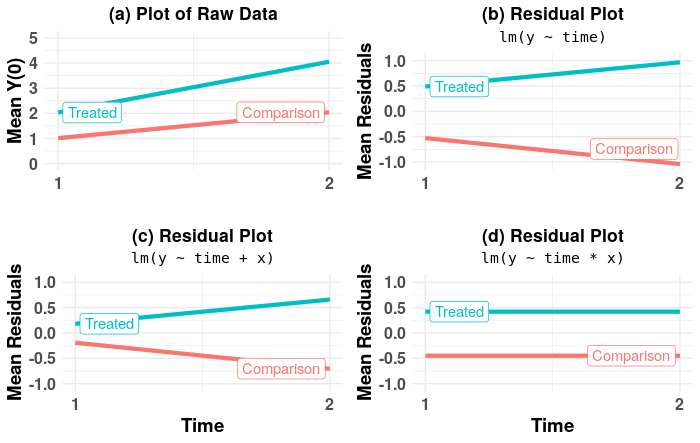
Figure 1: Adjusting for the main effect of a covariate does not correct for diverging trends, but adjusting for the interaction with time does in a simulated example where untreated potential outcomes depend on a time-invariant covariate with a time-varying effect. Panel (a) shows untreated potential outcomes. Panels (b)-(d) show residuals from linear models. The function lm— fits a linear model with outcome y—. In panel (b), the only predictor is time. In panel (c), the predictors are the main effects of time and the covariate. In panel (d), the predictors are time, the covariate, and an interaction between the two.

3.2 Adjusting for Time-Varying Confounders

Like time-invariant confounders, time-varying confounders invalidate parallel trends and introduce bias into our estimate of the ATT. If we were to adjust for time-varying confounding either by including the main effect or its interaction with time in a regression, we risk conditioning on post-treatment covariates that may be affected by treatment. As Rosenbaum (1984) notes for observational data, at best adjusting for post-treatment covariates provides no benefit; at worst, it may introduce additional bias. This is because the time-varying covariate can act as both a confounder and as a mediator. As such, when trying to recover the ATT via regression, the usual interaction parameter may not be an unbiased estimate of the ATT.

To see why this is the case, imagine three different scenarios: (a) the time-varying covariate changes in a way completely unrelated to treatment, (b) the time-varying covariate changes in a way wholly determined by treatment, and (c) the time-varying covariate changes in a way determined by a combination of treatment and other factors. Whenever (b) or (c) is true and the time-varying covariate is a cause of the outcome, the ATT is a combination of the direct effect of treatment and the indirect effect of treatment via the covariate. As a result the regression parameter on the interaction between treatment and the post-treatment indicator may not equal the ATT, even adjusted for the time-varying covariate. However, if we fail to account for the covariate, we face parallel trends violations. For a more detailed explanation, please see Appendix Section A.

In the causal inference literature, g-methods were specifically designed to deal with time-varying confounding (Hernan & Robins, 2019). A handful of papers incorporate these techniques into the diff-in-diff framework such as inverse probability weighting (Stuart et al., 2014; Han et al., 2017). However, only one employs inverse probability weighting to account for changes in covariate distributions across time (Stuart et al., 2014). In that paper, the authors consider a two time point/two group setting and define a new variable with four levels (treatment group in the pre-treatment period, treatment group in the post-treatment period, etc.). However, this methodology was only demonstrated on data with two time points and it should be noted that the target estimand changes from the classic ATT to an average treatment effect defined in the treatment group at the first time point. Nevertheless, it remains one of the only diff-in-diff papers to directly address the issue of time-varying confounders. In this paper, we use simulations to demonstrate that the estimate of the ATT is biased when time-varying covariates are affected by treatment, whether we adjust for the time-varying covariate or not (see Scenario 6 of Section 4.2).

3.3 What about Matching?

Matching aims to reduce confounding bias by selecting units from the treated and comparison groups that have similar observable characteristics. This eliminates imbalances between the groups, which is a key ingredient in confounding. When matching, we can match observations on pre-treatment outcomes, pre-treatment covariates, or some combination.

Matching on pre-treatment outcomes allows us to use an alternative assumption to identify the target parameter. This assumption — independence between potential outcomes and treatment assignment conditional on past outcomes — is the basis of lagged dependent variables regression and synthetic control methods (Lechner, 2011; O’Neill et al., 2016; Ding & Li, 2019). However, matching on pre-treatment outcomes in diff-in-diff can yield unwanted results. In some settings, it reduces bias (Stuart et al., 2014; Ryan et al., 2015), while in others, matching induces regression to the mean and creates bias (O’Neill et al., 2016; Daw & Hatfield, 2018).

Matching only on time-invariant pre-treatment covariates is attractive because it removes differences in the covariate distribution between the groups. With time-varying covariates, the picture is more complicated. Matching on time-varying pre-treatment covariates is subject to the same threat of bias due to regression to the mean as matching on pre-treatment outcomes. Moreover, if confounding arises because of differential evolution of the covariate in the two groups, matching only on pre-treatment values will be insufficient to address the confounding. Thus, we may wish to match on both pre- and post-treatment values of a time-varying covariate. In this case, we must also be wary of the dangers of matching on post-treatment variables that may be affected by treatment (Rosenbaum, 1984). Clearly, choosing the right matching variables is the key to effective matching. A good overview on the current state of matching for diff-in-diff is provided by Lindner & McConnell (2018).

Returning to the demonstration of parallel trends in Figure 1, matching on the pre-treatment covariate also serves to fix diverging trends. Recall that the data-generating model was a time-invariant covariate with a time-varying effect on the outcome. Eliminating the difference between the covariate means in the treated and comparison group via matching is sufficient to address confounding. If the confounding had arisen due to a time-varying covariate, the strategy may not suffice.

Both matching and regression adjustment have potential pitfalls. In addition to the possible regression to the mean problem mentioned above, we can mistakenly match on noise or on a set of covariates that is insufficient to alleviate bias in our causal effect. Furthermore, matching choices are largely ad hoc and can depend on the data structure itself. For example, it’s much more straightforward to match in panel data than in repeated cross-sections. Regression adjustment is not without its limitations as well. We can overfit our model, for one. We can also choose the wrong covariates to include or mispecify the functional form of the model. Deciding whether to address diverging trends through matching or regression or both must be done carefully. For example, say we are missing a key covariate that we suspect drives divergent trends, we cannot address the bias through regression adjustment and could instead consider matching on pre-treatment outcomes as a proxy for the missing covariate. On the other hand, if we have repeated cross-sectional data and it’s not clear how to match effectively, we can choose regression adjustment.

4 Simulations

We use simulation to compare regression adjustment and matching strategies in diff-in-diff. In each simulation scenario, we generate 400 datasets of $n=800$ units observed at $T=10$ time points. The first 5 time points are pre-treatment times, and the last 5 are post-treatment. Each unit is assigned to the treatment group with probability 0.5. To each simulated data set, we apply regression and matching techniques that reflect current practice in the applied literature and compare the bias of the resulting treatment effects.

We simulate data and analyze it using the R environment (R version 3.6.1 (R Core Team, 2019)). We fit regression models using the lm function and estimate post-hoc cluster-robust standard errors using the cluster.vcov function in the multiwayvcov package (Graham et al., 2016). To match, we use the MatchIt package (Ho et al., 2011). We present averages, across simulated data sets, of the percent bias and standard error of the estimated treatment effect.

Below, we describe the specifics of our data-generating and analysis models, first for scenarios with time-invariant covariates and then for scenarios with time-varying covariates.

4.1 Time-Invariant Covariate

4.1.1 Data-generating models

Scenario	Data-Generating Model
1: Time-invariant covariate effect	$X_{i}\stackrel{{\scriptstyle ind}}{{\sim}}N\left(m(a_{i}),v(a_{i})\right)$
	$Y_{i}(t)\stackrel{{\scriptstyle ind}}{{\sim}}N\left(1+a_{i}+a_{i}p_{t}+u_{i}+x_{i}+f(t),1\right)$
2: Time-varying covariate effect	$X_{i}\stackrel{{\scriptstyle ind}}{{\sim}}N\left(m(a_{i}),v(a_{i})\right)$
	$Y_{i}(t)\stackrel{{\scriptstyle ind}}{{\sim}}N\left(1+a_{i}+a_{i}p_{t}+u_{i}+x_{i}+f(t)+g(x_{i},t),1\right)$
3: Treatment-independent covariate	$X_{i}\stackrel{{\scriptstyle iid}}{{\sim}}N\left(1,1\right)$
	$Y_{i}(t)\stackrel{{\scriptstyle ind}}{{\sim}}N\left(1+a_{i}+a_{i}p_{t}+u_{i}+x_{i}+f(t)+g(x_{i},t),1\right)$

Table 1: Data-generating models with a time-invariant covariate, $x_{i}$. $Y_{i}(t)$: outcome for $i^{th}$ subject at time $t$. $a_{i}$: group indicator. $u_{i}$: random intercept. $p_{t}$: indicator of post-treatment time point. The treatment assignment for all scenarios is $a_{i}\stackrel{{\scriptstyle iid}}{{\sim}}\text{Bernoulli}(0.5)$ and the unit-level intercepts are all $u_{i}\stackrel{{\scriptstyle iid}}{{\sim}}N(0,.25^{2})$. $m(a_{i})=1.5-0.5a_{i}$, $f(t)=(t-2.5)^{2}/10$, $g(x_{i},t)=(x_{i}\cdot t)/10$, $v(a_{i})=(1.5-0.5a_{i})^{2}$.

Our first set of simulations involves a time-invariant covariate. In Scenario 1, the distribution of $X$ is different in the treated and control groups, but $X$ has a time-invariant effect on the outcome $Y$. Scenario 2 is the same as Scenario 1 but we allow the effect of $X$ on $Y$ to vary over time. In Scenario 3, the effect of $X$ on the mean of $Y$ is again time-varying, but the distribution of $X$ is the same in the treated and control groups. Table 1 summarizes the data-generating processes for these three simulations

We expect that in Scenarios 1 and 3, anlyses that do not adjust for $X$ will be unbiased, because $X$ does not satisfy the definition of a confounder. In Scenario 1, this is because $X$ does not have a time-varying effect on $Y$; in Scenario 3, this is because the distribution of $X$ is the same in both groups. In Scenario 2, we expect that only analyses that adjust appropriately for the time-varying effect of $X$ on $Y$ will yield unbiased results. For all three scenarios, the ATT equals the regression parameter which was set to 1. We measure bias with respect to this true ATT.

4.1.2 Analysis approaches

We use both matched and unmatched regression to analyze the simulated data. All regression models include time fixed effects and indicators for treatment, the post-period, and their interaction. The simple model includes only those elements, ignoring the covariate entirely. The covariate adjusted (CA) model adjusts for the covariate using a constant effect on the outcome over time. The time-varying adjusted (TVA) model allows the coefficient on the covariate to vary over time.

Our matching strategies include matching on both outcomes and covariates. We use nearest-neighbor matching on 1) the vector of pre-treatment outcomes, 2) the vector of pre-treatment outcome first differences, or 3) pre-treatment covariates. To each matched dataset, we fit a simple model without covariate adjustment. Table 2 describes the adjustment methods and gives pseudo code for each.

Model	Pseudo R code
Simple	lm(y ~ a*p + t)
Covariate-Adjusted (CA)	lm(y ~ a*p + t + x)
Time-Varying Adjusted (TVA)	lm(y ~ a*p + t*x)
Match on pre-treatment outcomes	lm(y ~ a*p + t,data=out.match)
Match on pre-treatment first differences	lm(y ~ a*p + t,data=out.lag.match)
Match on pre-treatment covariates	lm(y ~ a*p + t,data=cov.match)

Table 2: Analysis methods applied to each simulation scenario. The function lm— fits a linear model for outcome y—, treatment group indicator a—, post-treatment period indicator p—, (factor-coded) time t—, and covariate x—. The notation p*q— yields main effects for p— and q— plus their interaction.

4.2 Time-Varying Covariate

4.2.1 Data-generating models

The second set of simulations involves a time-varying covariate, with means that may evolve differently in the treated and comparison groups. The basic setup of these simulations (i.e., the number of units, time points, and treatment assignment) is the same as in Scenarios 1 through 3 above. We include three types of covariate evolution. In Scenario 4, the covariate evolves the same for both the treated group and the comparison group; in Scenario 5, the covariate evolves differently starting from baseline (related to treatment group, not treatment itself); and in Scenario 6, the covariate evolves the same in the two groups before treatment but differently after treatment.

For all these scenarios, we have two outcome processes: (a) the covariate has a time-invariant effect of the outcome and (b) the covariate has a time-varying effect on the outcome. Each scenario embeds two sub-scenarios, for a total of six data-generating processes. The data-generating distributions are summarized in Table 3. For Scenarios 4 and 5, the ATT equals the regression parameter (set to 1) as it did in Scenarios 1 through 3. However, Scenario 6 has a covariate that is changed by treatment, acting in part as a mediator. Thus, for Scenario 6, the ATTs are 0.85 and 0.87 for outcome processes (a) and (b), respectively. Work showing these calculations is provided in Appendix Section B. For all scenarios, we measure bias relative to the true ATT.

Scenario	Data-Generating Model
4: Parallel evolution	$X_{ti}=x_{(t-1)i}+m_{1}(t)\cdot z$
	$Y_{i}(t)\stackrel{{\scriptstyle ind}}{{\sim}}N\left(1+a_{i}+a_{i}p_{t}+u_{i}+x_{ti}+f(t)+g(x_{i},t),1\right)$
5: Evolution differs by group	$X_{ti}=x_{(t-1)i}+m_{2}(a_{i},t)\cdot z$
	$Y_{i}(t)\stackrel{{\scriptstyle ind}}{{\sim}}N\left(1+a_{i}+a_{i}p_{t}+u_{i}+x_{ti}+f(t)+g(x_{i},t),1\right)$
6: Evolution diverges in post	$X_{ti}=x_{(t-1)i}+m_{1}(t)\cdot z-m_{3}(a_{i},t)$
	$Y_{i}(t)\stackrel{{\scriptstyle ind}}{{\sim}}N\left(1+a_{i}+a_{i}p_{t}+u_{i}+x_{ti}+f(t)+g(x_{i},t),1\right)$

Table 3: Data-generating models with time-varying covariates, $x_{ti}$. $Y_{i}(t)$: outcome for $i^{th}$ subject at time $t$. $a_{i}$: group indicator. $u_{i}$: random intercept. $p_{t}$: indicator of post-treatment time point. The treatment assignment for all scenarios is $a_{i}\stackrel{{\scriptstyle iid}}{{\sim}}\text{Bernoulli}(0.5)$, the unit-level intercepts are $u_{i}\stackrel{{\scriptstyle iid}}{{\sim}}N(0,.25^{2})$, the covariate value at the first time point is $X_{1i}\stackrel{{\scriptstyle ind}}{{\sim}}N\left(1.5-0.5a_{i},(1.5-0.5a_{i})^{2}\right)$, and $z\stackrel{{\scriptstyle iid}}{{\sim}}N(1,0.1^{2})$. The functions that govern the evolution of the covariate are $m_{1}(t)=(t-1)/10$, $m_{2}(a_{i},t)=(I_{a_{i}=1}-I_{a_{i}=0})(t-1)/10$, and $m_{3}(a_{i},t)=a_{i}p_{t}t/20$. Outcome process (a) uses $f(t)=(t-2.5)^{2}/10$ and $g(x_{i},t)=0$. Outcome process (b) uses $f(t)=(t-2.5)^{2}/10$ and $g(x_{i},t)=(x_{i}\cdot t)/10$.

4.2.2 Analysis approaches

The analysis methods are the same as in Section 4.1.2 and Table 2, except that for these scenarios with a time-varying covariate, we match on the vector of pre-treatment covariate values.

4.3 Simulation Results

4.3.1 Time-Invariant Covariate

Figure 2: Simulation Results for Time-Invariant Covariate. CA = Covariate adjusted; TVA = Time-varying adjusted.

Figure 2 shows the results of fitting the models in Table 2 to the data generated from the time-invariant covariate data-generating models in Table 1. In Scenario 1, while $X$ is associated with treatment, it is not a confounder because the effect does not vary over time. Thus, the unadjusted analysis (simple model) is unbiased and adjusting for $X$ in the CA and TVA models does not affect either bias or standard errors. The results from our matched regressions are similar to those from the unmatched regressions.

In Scenario 2, the time-varying effect of $X$ on $Y$ makes $X$ a confounder and thus requires covariate adjustment with a time-varying aspect. Adjusting for the main effect of $X$ (CA model) does not alleviate bias or reduce the estimate’s standard error. Fortunately, we can address the bias by adjusting for the interaction of $X$ with time (TVA model). Of the matching strategies, only matching on the covariate effectively eliminates bias.

In Scenario 3, the simple model is already unbiased because $X$ is not a confounder. In fact, all estimation strategies yield unbiased estimates except matching on pre-treatment outcomes, which is biased by about 10 percent due to regression to the mean. We see about 20% lower mean standard error when we adjust for the covariate in the TVA model compared to the simple model.

4.3.2 Time-Varying Covariate

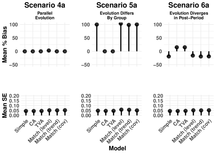
Figure 3: Simulation Results for Time-Varying Covariate. CA = Covariate adjusted; TVA = Time-varying adjusted.

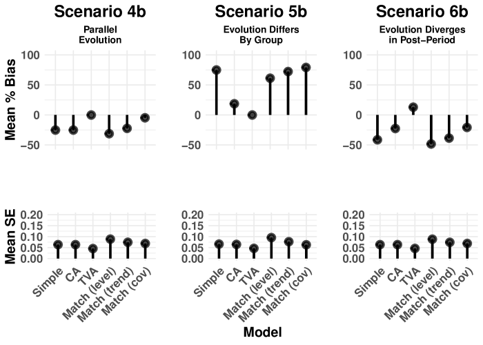
Figure 4: Simulation Results for Time-Varying Covariate. CA = Covariate adjusted; TVA = Time-varying adjusted.

Figures 3 and 4 show the results of fitting the models in Table 2 to the data generated using time-varying covariate processes (Table 3). In Scenario 4, there is no confounding when the effect of $X$ on $Y$ is constant over time, and the mean of $X$ evolves the same for each group. As a result, each modeling strategy is unbiased. However, when $X$ has a time-varying effect on $Y$, $X$ is a confounder and only time-varying adjustment (TVA) eliminates bias. Matching on the vector of pre-treatment values of $X$ nearly eliminates the bias.

In Scenario 5, the time-varying covariate evolves differently by group, beginning at baseline. When the effect of $X$ on the outcome is constant, we can simply adjust for time-varying $X$ (CA model) to eliminate confounding bias. When the effect of $X$ on $Y$ varies over time, we must adjust for the interaction of $X$ and time (TVA model). All of the matching strategies have significant bias.

In Scenario 6, the time-varying covariate evolves differently by group, but only after the treatment is introduced at $t=6$. Recall that in this scenario, the ATT does not simply equal the regression coefficient on an interaction term. As a result in Scenario 6, we have significant bias in our estimates and never succeed in recovering the true ATT.

5 Discussion

Diff-in-diff applications and methods have expanded dramatically over the past few decades. We contribute to this growing literature by examining how observable covariates may violate causal assumptions and comparing regression strategies to adjust for violations. It is tempting to toss all observed covariates into a regression model, but the form of the model specification should be tailored to address time-varying confounding.

Our methods and conclusions have several limitations. First, adjusting for confounders spends degrees of freedom, which may be untenable for sparse data. Second, regression adjustment depends on knowing and measuring the confounders as well as the functional form of their effects on the outcome (or having sufficient data to model it flexibly). Third, our conclusions only apply to linear models; nonlinear models are more complicated (Karaca-Mandic et al., 2012).

Done properly, regression adjustment can address bias caused by diverging trends. Further, even in the absence of confounding, adjusting for covariates can improve efficiency of the effect estimate (see Scenario 3 of Figure 2). And a correctly specified regression approach avoids conditioning on pre-treatment outcomes and so is not susceptible to regression to the mean in the same way that some matching methods are (Daw & Hatfield, 2018). Lastly, our regression adjustment strategy is agnostic to the structure of the data, whether panel data versus repeated cross-sections. Our simulations assumed panel data but our results will hold for repeated cross-sections. Matching on repeated cross-sections is trickier, since some covariates will necessarily be measured on different subjects at different time points, but it is possible (Keele et al., 2019).

For researchers using diff-in-diff in applied work, we recommend several steps for addressing confounding. First, researchers should clearly specify their model and explain how the inclusion of covariates and their functional forms support the researcher’s assumptions and model. This begins with writing out the full model specification and by providing analysis code in supplementary materials. Each covariate and coefficient should correspond to a threat to the validity of parallel trends and provide a valid remedy. We also recommend researchers comprehensively list covariates — both observed and unobserved — that might cause violations of parallel trends. The list should contain information on whether the variable is observed, whether the distribution of the covariate is expected to differ in the treatment and comparison groups, whether the covariate is time-varying, and whether it has an effect on the outcome. Depending on the application, we can use such a list to inform analysis choices. For example, if many unobserved covariates are a concern, the analyst may choose a different estimator (instead of one that relies on diff-in-diff and the parallel trends assumption). On the other hand, a single time-invariant covariate suggests a straightforward regression approach. Approaching both measured and unmeasured covariates illuminates the crucial causal assumptions underlying diff-in-diff more so than any test of parallel pre-treatment outcomes (Bilinski & Hatfield, 2018). Other authors have given similar advice, stressing attention to the reasons for baseline differences between the treated and comparison groups and how these differences might affect parallel trends (Kahn-Lang & Lang, 2018).

Being thorough in our diff-in-diff studies will strengthen conclusions and help alleviate concerns on the credibility of parallel trends. We expect diff-in-diff to continue its critical role in informing policy decisions into the foreseeable future. Going forward, it is crucial that diff-in-diff methodology is developed with input from statisticians, epidemiologists, economists, political scientists, and policy analysts alike.

Appendix A - Adjusting for Time-Varying Covariates

In this section of the appendix, we discuss of the problems of adjusting for time-varying confounders as described in Section 3.2 in the main paper. The thesis of our argument is that a time-varying covariate that is *affected* by treatment and also affects the outcome makes recovering the causal effect difficult. On one hand, failing to adjust for the time-varying covariate will result in failures of parallel trends. On the other hand, adjusting for the time-varying covariate, since it is on the pathway between treatment and the outcome, will negate some of the effect of treatment on the outcome, resulting in biased estimates.

We begin with notation that should be familiar to those who read our paper. $Y(t)$ is the continuous outcome measured at time $t$. For simplicity, we assume that $t\in\{0,1\}$ where $t=0$ is the pre-treatment period and $t=1$ the post-treatment period. Treatment is binary and represented by $A$. Finally, we have a time-varying covariate $X_{it}$ where $i$ in an index for a unit (e.g., a state or an individual). Let $\tau_{at}=E[X_{it}\mid A=a]$ be the covariate group-time mean. We also introduce counterfactual notation for the covariate so that $X^{a}_{it}$ is the (possibly counterfactual) value of $X$ for individual $i$ and time $t$ under treatment $A=a$. Since we assume that treatment directly affects $X$, we may have that $X^{0}_{i1}\neq X^{1}_{i1}$.

Let’s extend the notation for the covariate means to counterfactual world so that $E(X^{0}_{it}\mid A=a)=\tau^{0}_{at}$ and $E(X^{1}_{it}\mid A=a)=\tau^{1}_{at}$. We assume that treatment (which occurs between times 0 and 1) does not affect past versions of $X$ so that $\tau^{0}_{a0}=\tau^{1}_{a0}=\tau_{a0}$. We also assume that the covariate evolves differently in the two groups even absent treatment, leading to the failure of parallel trends. That is, $\tau_{01}-\tau_{00}\neq\tau_{11}-\tau_{10}$.

Suppose we have the same model for untreated outcomes as the main text:

$$E\left[Y_{i}^{0}(t)|A=a_{i},X^{0}=x^{0}_{it}\right]=\alpha_{0}+\alpha_{1}a_{i}+\zeta_{t}+\lambda_{t}x^{0}_{it}.$$

For simplicity, let $\lambda_{t}=\lambda$. We can connect the untreated outcomes to the treated outcomes with a fixed treatment effect, $\gamma$: $Y_{i}^{1}(t)=Y_{i}^{0}(t)+\gamma\;.$

Recall that the average treatment effect on the treated (ATT) is

$$ATT=E\left\{Y^{1}(1)-Y^{0}(1)\mid A=1\right\}\;.$$

Now, we have:

$$E\left\{Y^{1}(1)\mid A=1\right\}=\alpha_{0}+\alpha_{1}+\zeta_{1}+\lambda_{1}\tau^{1}_{11}+\gamma$$

and

$$E\left\{Y^{0}(1)\mid A=1\right\}=\alpha_{0}+\alpha_{1}+\zeta_{1}+\lambda_{1}\tau^{0}_{11}.$$

Plugging into the ATT:

$$ATT=\lambda_{1}\tau^{1}_{11}+\gamma-\lambda_{1}\tau^{0}_{11}=\gamma+\lambda_{1}(\tau^{1}_{11}-\tau^{0}_{11}).$$

The ATT is what we want to calculate, but what is our estimate for an unadjusted model versus one from a regression model that correctly adjusts for $X$.

Unadjusted Estimator:

$$\hat{ATT}_{unadj} =\left\{E\left(Y(1)\mid A=1\right)-E\left(Y(0)\mid A=1\right)\right\}-\left\{E\left(Y(1)\mid A=0\right)-E\left(Y(0)\mid A=0\right)\right\}$$

$$=\left\{\alpha_{0}+\alpha_{1}+\zeta_{1}+\lambda_{1}\tau_{11}+\gamma-(\alpha_{0}+\alpha_{1}+\zeta_{0}+\lambda_{0}\tau_{10})\right\}-$$

$$\ \ \ \ \left\{\alpha_{0}+\zeta_{1}+\lambda_{1}\tau_{01}-(\alpha_{0}+\zeta_{0}+\lambda_{0}\tau_{00})\right\}$$

$$=\gamma+\zeta_{1}-\zeta_{0}+\lambda_{1}\tau_{11}-\lambda_{0}\tau_{10}-(\zeta_{1}-\zeta_{0}+\lambda_{1}\tau_{01}-\lambda_{0}\tau_{00})$$

$$=\gamma+\lambda_{1}\tau_{11}-\lambda_{0}\tau_{10}-\lambda_{1}\tau_{01}+\lambda_{0}\tau_{00}$$

$$=\gamma+\lambda_{1}(\tau_{11}-\tau_{01})-\lambda_{0}(\tau_{10}-\tau_{00}).$$

Without significant restrictions on the $\lambda$ and $\tau$ values, this does not equal the ATT.

Adjusted Estimator:

Now, imagine we know which regression model to fit. In R, we can fit the model lm(y~a*t + x*t), which is correctly specified. The estimate of the treatment effect will be the coefficient on the interaction between a (treatment indicator) and t (time). However, when we fit the model, we will get:

$$\hat{ATT}_{adj}=\gamma,$$

which is biased for the true ATT.

Appendix B - Calculation of ATT for Simulation Scenario 6

In the main paper, we state that the average treatment effect on the treated (ATT) in Scenario 6 is different than in the other scenarios. Here, we show our calculations for the ATT using our data-generating example. Below is the code used to generate data, using the dplyr R package.

dat <- expand.grid(id = 1:n, tp = 1:max.time) %>%
    arrange(id,tp) %>% group_by(id) %>%
    mutate(int=rnorm(1,0,sd=0.25), # random intercept
           p.trt=0.5, # probability of treatment
           trt=rbinom(1, 1, p.trt), # treatment
           x=rnorm(1, mean = 1.5 - 0.5*trt, sd = 1.5 - 0.5*trt),
           post=I(tp >= trt.time), # indicator of post-treatment period
           treated=I(post == 1 & trt == 1), # treated indicator
           x=ifelse(tp>=2, lag(x, 1) + (tp-1)/10 *
                rnorm(1, mean = 1, sd = 0.1) -
                I(trt == 1) * I(tp>6)*(tp)/20, x)
    ) %>%
    ungroup()

dat <- dat %>% mutate(err=rnorm(n*max.time),
                      y = 1 + x + trt + int + err + treated +
ΨΨ       ((tp - 2.5)^2)/10,
                      y.t =  1 + x * tp / 10 + trt +
                             int + err + treated + ((tp - 2.5)^2)/10) %>%
    group_by(id) %>%
    mutate(y.diff = y - lag(y), y.diff2 = y.t - lag(y.t)) %>%
    ungroup()

To begin, we only need to look at the treated group since the ATT is defined on the treated population. The setup is relatively simple. We set $n=1000$ to be the total number of units followed over 10 (max.time) time points. Units were assigned to the treatment group with probability $0.5$. The treated units were given treatment beginning at $t=6$; thus, we had five pre-treatment time points and five post-treatment time points. The covariate $X$ at baseline was drawn from a Normal distribution, $N(1,1^{2})$ from the treated population. During the pre-treatment period, the means of the covariate increased by about $\frac{1}{10}$ cumulatively from $t=2,\dots,10$. However, the mean of the covariate was affected by treatment too, so that for the treated group when $t\geq 6$, the mean went down by an average of $\frac{1}{20}$ per time point.

Time	$t=1$	$t=2$	$t=3$	$t=4$	$t=5$	$t=6$	$t=7$	$t=8$	$t=9$	$t=10$
Mean($X^{0}$)	1.0	1.1	1.2	1.3	1.4	1.5	1.6	1.7	1.8	1.9
Mean($X^{1}$)	1.0	1.1	1.2	1.3	1.4	1.45	1.5	1.55	1.6	1.65

Table B1: Evolution of counterfactual means of covariate $X$ for the treated group.

Note that for this simulation scenario, we have two different outcomes. In the first, denoted y, the effect of $X$ on the outcome is the same at every time point. For the second outcome, denoted y.t, the covariate has a time-varying effect on the outcome. The two outcome processes are detailed below:

$$y =1+x+trt+int+err+treated+((tp-2.5)^{2})/10$$

$$y.t =1+x*tp/10+trt+int+err+treated+((tp-2.5)^{2})/10).$$

So this difference is that in the second equation, $X$ interacts with time. Note that both $int$ and $err$ are mean zero normal random variables and $treated=1$ whenever $tp>5$. (We are only considering the treated group. This would not be true for the comparison group.) Like we did for the mean of $X$, we can build a table for the means of $Y$ using the above equations.

For y, we get the following results:

Time	$t=1$	$t=2$	$t=3$	$t=4$	$t=5$	$t=6$	$t=7$	$t=8$	$t=9$	$t=10$	Avg. pre	Avg. post
Mean($Y^{0}$)	3.225	3.125	3.225	3.525	4.025	4.725	5.625	6.725	8.025	9.525	3.425	6.925
Mean($Y^{1}$)	3.225	3.125	3.225	3.525	4.025	5.675	6.525	7.575	8.825	10.275	3.425	7.775

Table B2: Evolution of counterfactual means of outcome $Y$ for the treated group.

We’ll calculate a few of these by hand to give an idea of what we’re doing. Take the mean of $Y^{0}$ at $t=7$:

$$y =1+x+trt+int+err+treated+((tp-2.5)^{2})/10$$

$$=1+x+1+0+0+0+(7-2.5)^{2}/10$$

$$=1+1.6+1+0+0+0+(7-2.5)^{2}/10$$

$$=5.625.$$

Here, we plugged in 1.6 for $x$ since it equals the untreated mean of the covariate (see Table B1). Both $int$ and $err$ are independent mean zero random variables so we plug in 0.

Following similar calculations, the mean of $Y^{1}$ at $t=7$ is:

$$y =1+x+trt+int+err+treated+((tp-2.5)^{2})/10$$

$$=1+x+1+0+0+1+(7-2.5)^{2}/10$$

$$=1+1.5+1+0+0+1+(7-2.5)^{2}/10$$

$$=6.525.$$

The ATT here is $7.775-6.925=0.85$, which is calculated by taking the mean of the last 5 columns (the post-treatment time points) for each row and subtracting them.

And for y.t, we get the following results:

Time	$t=1$	$t=2$	$t=3$	$t=4$	$t=5$	$t=6$	$t=7$	$t=8$	$t=9$	$t=10$	Avg. pre	Avg. post
Mean($Y^{0}$)	2.325	2.245	2.385	2.745	3.325	4.125	5.145	6.385	7.845	9.525	2.605	6.605
Mean($Y^{1}$)	2.325	2.245	2.385	2.745	3.325	5.095	6.075	7.265	8.665	10.275	2.605	7.475

Table B3: Evolution of counterfactual means of outcome $Y$ for the treated group.

The ATT here equals 0.87.

References

- (1)
- Abadie (2005) Abadie, A. (2005), ‘Semiparametric difference-in-differences estimators’, Review of Economic Studies 72, 1–19.
-
Angrist & Pischke (2008)
Angrist, J. D. & Pischke, J.-S. (2008), Mostly Harmless Econometrics: An
Empiricist’s Companion, Princeton University Press, Princeton, NJ.
http://www.mostlyharmlesseconometrics.com/ -
Antonisse et al. (2018)
Antonisse, L., Garfield, R., Rudowitz, R. & Artiga, S.
(2018), The effects of medicaid expansion
under the aca: Updated findings from a literature review, Technical report,
Henry J Kaiser Family Foundation (KFF).
https://www.kff.org/medicaid/issue-brief/the-effects-of-medicaid-expansion-under-the-aca-updated-findings-from-a-literature-review-march-2018/ - Bai (2009) Bai, J. (2009), ‘Panel data models with interactive fixed effects’, Econometrica 77(4), 1229–1279.
-
Bilinski & Hatfield (2018)
Bilinski, A. & Hatfield, L. A. (2018), ‘Seeking evidence of absence: Reconsidering tests
of model assumptions’, arXiv:1805.03273 [stat] .
arXiv: 1805.03273.
http://arxiv.org/abs/1805.03273 - Blavin (2016) Blavin, F. (2016), ‘Association between the 2014 Medicaid expansion and us hospital finances’, JAMA 316, 1475–1483.
-
Bradford et al. (2018)
Bradford, A. C., Bradford, W. D., Abraham, A. & Bagwell Adams, G.
(2018), ‘Association between US state
medical cannabis laws and opioid prescribing in the Medicare Part D
population’, JAMA Internal Medicine 178(5), 667.
http://archinte.jamanetwork.com/article.aspx?doi=10.1001/jamainternmed.2018.0266 -
Card & Krueger (1993)
Card, D. & Krueger, A. B. (1993),
Minimum wages and employment: A case study of the fast food industry in new
jersey and pennsylvania, Working Paper 4509, National Bureau of Economic
Research.
http://www.nber.org/papers/w4509 - Daw & Hatfield (2018) Daw, J. R. & Hatfield, L. A. (2018), ‘Matching and regression-to-the-mean in difference-in-differences analysis’, Health Services Research .
- Desai et al. (2016) Desai, S., Hatfield, L. A., Hicks, A. L., Chernew, M. E. & Mehrotra, A. (2016), ‘Association between availability of a price transparency tool and outpatient spending’, JAMA 315, 1874–81.
- Ding & Li (2019) Ding, P. & Li, F. (2019), ‘A bracketing relationship between difference-in-differences and lagged-dependent-variable adjustment’, arXiv preprint arXiv:1903.06286 .
- Graham et al. (2016) Graham, N., Arai, M. & Hagströmer, B. (2016), ‘multiwayvcov: Multi-way standard error clustering. r package version 1.2. 3’.
- Han et al. (2017) Han, B., Yu, H. & Friedberg, M. W. (2017), ‘Evaluating the impact of parent-reported medical home status on children’s health care utilization, expenditures, and quality: a difference-in-differences analysis with causal inference methods’, Health Serv Res 52, 786–806.
-
Hernan & Robins (2019)
Hernan, M. A. & Robins, J. M. (2019), Causal inference, CRC Boca Raton, FL.
https://www.hsph.harvard.edu/miguel-hernan/causal-inference-book/ -
Ho et al. (2011)
Ho, D. E., Imai, K., King, G. & Stuart, E. A. (2011), ‘MatchIt: Nonparametric preprocessing for
parametric causal inference’, Journal of Statistical Software 42(8), 1–28.
http://www.jstatsoft.org/v42/i08/ -
Kahn-Lang & Lang (2018)
Kahn-Lang, A. & Lang, K. (2018),
The promise and pitfalls of differences-in-differences: reflections on ‘16
and Pregnant’ and other applications, Technical Report 24857, National
Bureau of Economic Research, Cambridge, MA.
http://www.nber.org/papers/w24857 -
Karaca-Mandic et al. (2012)
Karaca-Mandic, P., Norton, E. C. & Dowd, B. (2012), ‘Interaction terms in nonlinear models’, Health
Services Research 47(1pt1), 255–274.
http://doi.wiley.com/10.1111/j.1475-6773.2011.01314.x - Keele et al. (2019) Keele, L. J., Small, D. S., Hsu, J. Y. & Fogarty, C. B. (2019), ‘Patterns of effects and sensitivity analysis for differences-in-differences’, arXiv preprint arXiv:1901.01869 .
- Kobayashi et al. (2019) Kobayashi, L. C., Altindag, O., Truskinovsky, Y. & Berkman, L. F. (2019), ‘Effects of the affordable care act medicaid expansion on subjective well-being in the us adult population, 2010–2016’, American journal of public health 109(9), 1236–1242.
- Lechner (2011) Lechner, M. (2011), ‘The estimation of causal effects by difference-in-difference methods’, Foundations and Trends® in Econometrics 4(3), 165–224.
-
Lindner & McConnell (2018)
Lindner, S. & McConnell, K. J. (2018), ‘Difference-in-differences and matching on outcomes:
a tale of two unobservables’, Health Services and Outcomes Research
Methodology .
http://link.springer.com/10.1007/s10742-018-0189-0 - McWilliams et al. (2014) McWilliams, J. M., Landon, B. E., Chernew, M. E. & Zaslavsky, A. M. (2014), ‘Changes in patients’ experiences in Medicare accountable care organizations’, The New England journal of medicine 371, 1715–24.
- National Federation of Independent Business v. Sebelius (2011) National Federation of Independent Business v. Sebelius (2011), www.oyez.org/cases/2011/11-393. Accessed: 2019-07-18.
- O’Neill et al. (2016) O’Neill, S., Kreif, N., Grieve, R., Sutton, M. & Sekhon, J. S. (2016), ‘Estimating causal effects: considering three alternatives to difference-in-differences estimation’, Health Serv Outcomes Res Methodol 16, 1–21.
-
R Core Team (2019)
R Core Team (2019), R: A Language and
Environment for Statistical Computing, R Foundation for Statistical
Computing, Vienna, Austria.
https://www.R-project.org/ -
Roberts et al. (2018)
Roberts, E. T., McWilliams, J. M., Hatfield, L. A., Gerovich, S., Chernew,
M. E., Gilstrap, L. G. & Mehrotra, A. (2018), ‘Changes in health care use associated with the
introduction of hospital global budgets in maryland’, JAMA Internal
Medicine 178(2), 260.
http://archinte.jamanetwork.com/article.aspx?doi=10.1001/jamainternmed.2017.7455 - Rosenbaum (1984) Rosenbaum, P. R. (1984), ‘The consequences of adjustment for a concomitant variable that has been affected by the treatment’, Journal of the Royal Statistical Society: Series A (General) 147(5), 656–666.
- Rosenthal et al. (2016) Rosenthal, M. B., Landrum, M. B., Robbins, J. A. & Schneider, E. C. (2016), ‘Pay for performance in Medicaid: Evidence from three natural experiments’, Health Services Research 51, 1444–66.
- Ryan et al. (2015) Ryan, A. M., Burgess, J. F. & Dimick, J. B. (2015), ‘Why we should not be indifferent to specification choices for difference-in-differences’, Health Services Research .
- Stuart et al. (2014) Stuart, E. A., Huskamp, H. A., Duckworth, K., Simmons, J., Song, Z., Chernew, M. E. & Barry, C. L. (2014), ‘Using propensity scores in difference-in-differences models to estimate the effects of a policy change’, Health Services and Outcomes Research Methodology 14(4), 166–182.
-
VanderWeele & Shpitser (2013)
VanderWeele, T. J. & Shpitser, I. (2013), ‘On the definition of a confounder’, The Annals
of Statistics 41(1), 196–220.
http://projecteuclid.org/euclid.aos/1364302740 - Xu (2017) Xu, Y. (2017), ‘Generalized synthetic control method: Causal inference with interactive fixed effects models’, Political Analysis 25(1), 57–76.