Bias-Induced Chiral Current and Topological Blockade in Triple Triangular Quantum Dots

Abstract

We theoretically investigate the quantum transport properties of a triangular triple quantum dot (TTQD) ring connected with two reservoirs by means of analytical derivation and accurate hierarchical–equations–of–motion calculation. A bias-induced chiral current in the absence of magnetic field is firstly demonstrated, which results from that the coupling between spin gauge field and spin current in the nonequilibrium TTQD induces a scalar spin chirality that lifts the chiral degeneracy and thus the time inversion symmetry. The chiral current is proved to oscillate with bias within the Coulomb blockade regime, which opens a possibility to control the chiral spin qubit by use of purely electrical manipulations. Then, a topological blockade of the transport current due to the localization of chiral states is elucidated by spectral function analysis. Finally, as a measurable character, the magnetoelectric susceptibility in our system is found about two orders of magnitude larger than that in a typical magnetoelectric material at low temperature.

In condensed matter physics, the geometric (Berry) phase coherence may strongly affect the charge dynamics. A case in point is the anomalous Hall effect in ferromagnetic metals, showing a nonzero transverse resistivity, even there is no external magnetic field. The geometric phase of Bloch wave functions plays a major role in this phenomenon [1]. A nontrivial spin texture in ferromagnetic metals produces a gauge flux that can be incorporated into transfer integrals by additional phase factors [2, 3]. In literature, this anomalous contribution had been attributed to the spin-orbit interaction and spin polarization of conduction electrons. In the strong Hund–coupling limit, the conduction electron spin aligns with the impurity spin. The resulted fictitious magnetic field, produced by the noncoplanar spin configuration or spin chirality [1, 4], gives rise to the Hall conductivity a topological origin. The fictitious magnetic field has a uniform component due to spin-orbit interactions [5, 6, 7].

Consider a minimal chiral spin model, as shown in Fig. 1(a), with three local spins, $\bm{S}_{1}$, $\bm{S}_{2}$ and $\bm{S}_{3}$, whose axes are tilted away from the overall magnetization axis. This triple triangular quantum dots (TTQDs) system is a nonmagnetic structure. However, when a conduction electron moves in the background of those spins, the phase factor picked up by this electron is given by $e^{i\Omega/2}$, where $\Omega$ is the solid angle subtended by the three spins on the unit sphere. The chiral spin state is closely related to chiral-spin-liquid and superconductivity states [8]. The geometric phase acts as the gauge field with two essential consequences. One is the anomalous Hall effect [1], and another is the chiral current of $I_{c}\propto\bm{S}_{1}(\bm{S}_{2}\times\bm{S}_{3})$. We will demonstrate how to obtain chiral current in a nonmagnetic TTQD structure without magnetic field; see Fig. 1(b)-(c). Moreover, we uncover a novel topological blockade effect due to this topological current.

TTQDs are composed of three coupled quantum dots in a triangle form, with two or three reservoirs connected to them. As the smallest artificial molecule with topological properties, TTQDs received extensive studies, both experimental [9, 10, 11, 12] and theoretical [13, 14, 15, 16, 17, 18, 19, 20]. They are prominent candidates for research on various quantum interference effects in the strong correlation regime [18, 20]. Remarkably, TTQDs have shown potential applications in quantum computing based on the qubits encoded in chiral spin states [21, 14, 15, 16]. The chiral qubit is embedded in a decoherence-free subspace and is immune to collective noises [22], and thus robust against random charge fluctuations [13].

However, the manipulation of chiral qubit or chiral spin state is challenging in general. Existing proposals [13, 14, 15, 16] engage a perpendicular magnetic field to split the degeneracy of left- and right-hand chiral states. Nevertheless, the application of external magnetic field would not be practical for quantum computing, due to its incompatibility with the large-scale integrated circuit. Moreover, it is generally very hard to localize the required oscillating magnetic fields for quantum gate or qubit manipulation.

In principle, an applied magnetic field is not a necessity since the gauge field from the aforementioned geometric phase could play the same role. Motivated by this insight, we propose the manipulation on the chiral qubit and chiral spin state via the bias–voltage induced chiral current. We will demonstrate this proposal with the Anderson triple-impurity model TTQDs that are accurately evaluated and thoroughly analyzed.

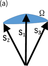
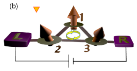
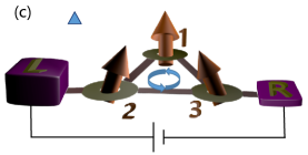
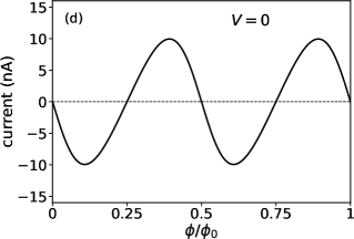
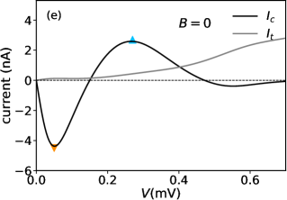
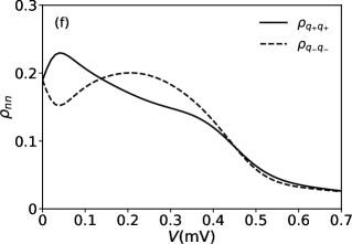
Figure 1: (color online) (a) Scalar spin chirality defined by the solid angle spanned by three spins. (b) Schematic diagram of the clockwise chiral current in the TTQD with two dots connected to reservoirs L and R, and (c) the anticlockwise counterpart. (d) Chiral current as a function of magnetic flux under equilibrium condition ($V=0$). (e) Chiral current $I_{c}$ versus transport current $I_{t}$ (thin-curve), as functions of bias voltage $V$, without magnetic flux ($B=0$). (f) The $V-$dependent populations, $\rho_{q_{+}q_{+}}$(solid curve) and $\rho_{q_{-}q_{-}}$(dash curve), in the two chiral states. The parameters are (in meV) $\epsilon=-0.5$, $U=1.0$, and $t=0.25$ for the TTQD system, $\Delta=0.025$ for the system–reservoirs coupling strength, and $k_{B}T=0.05$.

Figure 1(b) or (c) depicts our TTQD structure in a quantum transport setup. Each QD is in the local moment regime with a $\frac{1}{2}$-spin. The QD2 and QD3 couple to electronic reservoirs L and R, respectively. The total composite Hamiltonian, $H_{\rm T}=H_{\rm{dots}}+H_{\rm{res}}+H_{\rm{coup}}$, is described by the Anderson impurity model, in which

$$H_{\rm{dots}}=\sum_{j,k=1}^{3}\sum_{s=\uparrow,\downarrow}t_{jk}\hat{d}_{js}^{\dagger}\hat{d}_{ks}+\sum_{j=1}^{3}U_{j}\hat{n}_{j\uparrow}\hat{n}_{j\downarrow}.$$ (1)

Here, $\hat{n}_{js}\equiv\hat{d}_{js}^{\dagger}\hat{d}_{js}$ is the number operator for an electron occupying the specified on-dot spin–orbital. For clarity, let the TTDQ hold $C_{3v}$ symmetry, with $t_{12}=t_{23}=t_{31}=t$, whereas $U_{j}=U$ and $\epsilon_{j}\equiv t_{jj}=-U/2$ for the on-dot Coulomb repulsion and energy, respectively. The non-interaction Fermion reservoir is described by $H_{\rm{res}}=\sum_{\alpha\in{\rm L,R}}\sum_{\kappa s}(\epsilon_{\alpha\kappa s}+\mu_{\alpha})\hat{c}_{\alpha\kappa s}^{\dagger}\hat{c}_{\alpha\kappa s}$, with $\mu_{\rm L}=eV/2=-\mu_{\rm R}$ The TQD system–and–reservoir coupling is described by $H_{\rm{coup}}=\sum_{\kappa s}(t_{{\rm L}2}\hat{c}_{{\rm L}\kappa s}^{\dagger}\hat{d}_{2s}+t_{{\rm R}3}\hat{c}_{{\rm R}\kappa s}^{\dagger}\hat{d}_{3s}+{\rm H.c.})$.

In the following, we will first investigate the chiral current induced by a magnetic field applied to the isolated TTQD. By doing that, we unambiguously identify the chiral current operator, $\hat{I}_{c}$ [cf. Eq. (3)], which will also be used in the bias voltage–induced chiral current evaluations. Let us start with pristine TTQD in the absence of magnetic field and reservoirs. The ground state of the isolated TTQD is four-fold degenerate, with spin configuration being 120^∘ between neighboring spins without chirality. That is, the three spins are coplanar with the degenerate chiral states. When a perpendicular magnetic field is applied, a flux threads the ringlike TTQD structure. A $t$-$J$-$\chi$ Hamiltonian can be derived by treating $t$ in $H_{\rm{dots}}$ perturbatively [23, 24]:

$$H_{\rm{eff}} =-t(1-n)\sum_{jk,s}(\hat{d}_{js}^{\dagger}\hat{d}_{ks}+{\rm{H.c.}})$$

$$\quad\,+J\sum_{j<k}(\hat{\bm{S}}_{j}\hat{\bm{S}}_{k}-\frac{1}{4}\hat{n}_{j}\hat{n}_{k})+\chi\hat{\bm{S}}_{1}(\hat{\bm{S}}_{2}\times\hat{\bm{S}}_{3}).$$ (2)

Here, $n$ is the average electron occupation number on each dot. In the half-filling situation, the $t-$term vanishes due to $n=1$. The $J$-term is the usual Heisenberg exchange interaction, with $J=4t^{2}/U$. The last term is chiral, with $\chi=24t^{3}\sin(2\pi\phi/\phi_{0})/U^{2}$, where $\phi$ is the magnetic flux enclosed by the TTQD, and $\phi_{0}=hc/e$ is the unit of quantum flux. It has been shown that for TTQDs the chiral operator reads [8]

$$\hat{\bm{S}}_{1}(\hat{\bm{S}}_{2}\times\hat{\bm{S}}_{3})=\frac{1}{2i}\!\sum\limits_{suv}\!\hat{d}_{1s}^{\dagger}(\hat{d}_{2s}\hat{d}_{2u}^{\dagger}\hat{d}_{3u}\hat{d}_{3v}^{\dagger}-\hat{d}_{3s}\hat{d}_{3u}^{\dagger}\hat{d}_{2u}\hat{d}_{2v}^{\dagger})\hat{d}_{1v}.$$

It splits the four-fold degenerate ground state in the total spin-$\frac{1}{2}$ subspace into two chiral–states pairs. One is the minority spin circling clockwise ($+$) and anticlockwise ($-$) pair, $\ket{q_{\pm}}=\frac{1}{\sqrt{3}}(\ket{\uparrow\downarrow\downarrow}+e^{\pm\frac{i2\pi}{3}}\ket{\downarrow\uparrow\downarrow}+e^{\pm\frac{i4\pi}{3}}\ket{\downarrow\downarrow\uparrow})$. Another pair for $S_{z}=-1/2$ are similar but with all spins flipped. For $S_{z}$ degeneracy denote $\ket{q_{+}^{1/2}}$ as $\ket{q_{+}}$ for simplicity and that of $S_{z}=-1/2$ are of same values. These are the eigenstates of the TTQD chiral operator or the last term of Eq. (Bias-Induced Chiral Current and Topological Blockade in Triple Triangular Quantum Dots) that describes the electrons circular transfer difference between clockwise and anticlockwise directions. We identity the chiral current operator,

$$\hat{I}_{c}=-\frac{24e}{\hbar}\frac{t^{3}}{U^{2}}\hat{\bm{S}}_{1}(\hat{\bm{S}}_{2}\times\hat{\bm{S}}_{3}).$$ (3)

It follows the Hellman-Feynman theorem for chiral current, $I_{c}=-\frac{e}{\hbar}\langle\frac{\partial\hat{H}_{\rm{dots}}}{\partial{\phi}}\rangle=-\frac{e}{\hbar}\frac{\partial F_{\rm{dots}}}{\partial{\phi}}$, with $F_{\rm{dots}}$ being the magnetic field induced free–energy [25]. TTQD constitutes the shortest loop where each dot is in local moment region. The coefficient $t^{3}/U^{2}$ is the lowest-order nonvanishing contribution to the circling current. Figure Fig. 1(d) depicts the chiral current as a function of flux at equilibrium state. It shows a double period with flux. In short, the chiral operator breaks the symmetry of TTQD from $C_{3v}$ into $C_{3}$ and induces a chiral current.

Chiral current induced by bias voltage. We will elaborate below that for the open TTQDs, a finite applied bias voltage alone could also break the chiral symmetry and drive a nearly pure chiral current. Lai et al. report that away from local magnetic moment regime, internal charge current circulation can spontaneously emerge, with a non-monotonic behavior of transport current when the circulation reverses [26]. Here we focus on the electron transport in local moment regime, in which the phase coherence of spins plays an important role. Let us start with the accurate numerical results via the well–established hierarchical equations of motion (HEOM) approach [27, 28, 29, 30]. High-order tunneling processes such as cotunneling [19] and many-body tunneling [31] have been well handled by HEOM. The present TTQD in study has $\epsilon=-U/2=-0.5$ meV. The couplings between electrodes and TTQD are set to $\Gamma_{\rm L}=\Gamma_{\rm R}=\Delta=0.025$ meV. The temperature is $T=0.6$ K, which is far above the Kondo temperature that is about $T_{K}\sim 3.6\times 10^{-4}$ mK.

Figure 1(e) depicts the calculated chiral current $I_{c}$ as a function of bias voltage $V$. The resulted $I_{c}(V)$ shows oscillations at $V<U/2$. This is the Coulomb blockade regime for the present TTQD in study. Further increasing bias ($V>U/2$) will push the system out of the Coulomb blockade regime, where $I_{c}$ gradually decreases to zero and meantime the transport current $I_{t}$ increases.

Remarkably, our results show that it is possible to control the chiral spin qubit by use of purely electrical manipulations without magnetic field involved. In the Coulomb blockade regime ($V<U/2$), the lead–dressed ground state under bias would be the aforementioned chiral pairs $\{|q_{\pm}\rangle\}$; see Fig. 1(b) and (c). In particular, compared to the magnetic–field counterpart of Fig. 1(d), the bias–dressed states at $V=0.05$ and $0.25$ mV are associated with the maximal clockwise and anticlockwise chiral currents, respectively. Figure 1(f) reports the reduced density matrix diagonal elements, $\rho_{q_{+}q_{+}}$ and $\rho_{q_{-}q_{-}}$, for the two chiral states populations as function of bias. Evidently, the sign and magnitude of the difference, $\rho_{q_{+}q_{+}}-\rho_{q_{-}q_{-}}$, correlates well with the observed direction and magnitude of chiral current in Fig. 1(e). It is worth noting that the chiral ground states are degenerate, $\rho_{q_{+}q_{+}}=\rho_{q_{-}q_{-}}$, at $V=0.15$ meV. The resulted $I_{c}=0$ would have an effective magnetic flux of $\phi^{\rm eff}=\phi_{0}/4$. Physically this differs from the scenarios of $V>U/2$, beyond the Coulomb blockade regime, where $\phi^{\rm eff}\approx 0$ that is responsible for the observed $\rho_{q_{+}q_{+}}\approx\rho_{q_{-}q_{-}}$ and $I_{c}\approx 0$.

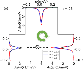
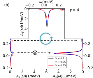
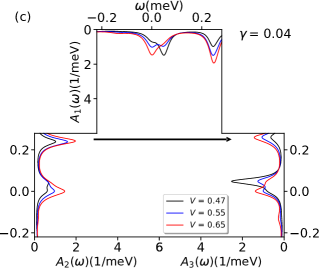
Figure 2: (color online) Nonequilibrium spectral functions, $A_{i}(\omega)=A_{is}(\omega)$, with $i=1,2,3$ and $s=\uparrow,\downarrow$, in the (a) blockade region ($0\leq V\leq 0.15$ mV), (b) coexistence region ($0.15<V\leq 0.4$ mV), and (c) conduction region ($0.4<V\leq 0.7$ mV). Indicated is also the calculated value of $\gamma\equiv\int_{\text{\tiny$V_{1}$}}^{\text{\tiny$V_{2}$}}\!|I_{c}|dV\big{/}\int_{\text{\tiny$V_{1}$}}^{\text{\tiny$V_{2}$}}\!I_{t}dV$ in each region.

Spin gauge field coupling analysis. The above observations can be analyzed and understood as follows. Bias breaks the inversion symmetry of the TTQD which is required for the coupling between spin gauge field and spin current. The Hubbard-Stratonovich approach is adopted to decouple the on-site Coulomb interaction in our Anderson impurity model, as described in detail in Supplemental Material [32]. To keep the spin rotation invariance, a unitary transformation in spin space, $\Phi_{j}=R_{j}\Psi_{j}$, is introduced. Here, $R_{j}$ is a site- and time-dependent SU(2) rotation matrix satisfying $\bm{\sigma}\bm{S}_{j}=R_{j}\sigma_{z}R_{j}^{\dagger}$. The electron operators are given in the spinor form, $\Psi_{j}^{\dagger}=(\hat{d}^{\dagger}_{j\uparrow},\hat{d}^{\dagger}_{j\downarrow})$. With the polar representation of the dot spin $\bm{S}=(\sin{\theta}\cos{\phi},\sin{\theta}\sin{\phi},\cos{\theta})^{T}$, the matrix $R=e^{\frac{i\pi}{2}}e^{-\frac{i\phi}{2}\sigma_{z}}e^{-\frac{i\theta}{2}\sigma_{x}}e^{-\frac{i(\pi-\phi)}{2}\sigma_{z}}$ rotates the spin up state $\ket{\uparrow}$ to the direction of dot spin as $\ket{\bm{S}}=R\ket{\uparrow}$. Consequently, the kinetic term of $H_{\rm{dots}}$ has a covariant form, since $t_{jk}\Psi_{j}^{\dagger}\Psi_{k}\rightarrow t_{jk}\Phi_{j}^{\dagger}R_{j}^{\dagger}(R_{k}-R_{j})\Phi_{k}$ and $\Psi_{j}^{\dagger}\partial_{\tau}\Psi_{j}\rightarrow\Phi_{j}^{\dagger}(\partial_{\tau}+R_{j}\partial_{\tau}R_{j})\Phi_{j}$. The SU(2) spin gauge field is defined through $A_{jk}\equiv-iR_{j}^{\dagger}(R_{k}-R_{j})$ and $A_{0j}\equiv R_{j}\partial_{\tau}R_{j}$. These can be expressed in terms of the Pauli matrices as $A_{jk}=\sum_{r}A_{jk}^{r}\sigma_{r}$, where $r=x,y,z$ is the direction in spin space. The gauge field couples to spin current through minimal coupling. The coupling energy reads

$$H_{A}=\sum_{jkr}j_{jk}^{r}A_{jk}^{r}+\sum_{jr}s_{j}^{r}A_{0j}^{r},$$ (4)

with $s_{j}^{r}=\Phi_{j}^{\dagger}\sigma_{r}\Phi_{j}$ and $j_{jk}^{r}=-\frac{iet}{\hbar}(\Phi_{j}^{\dagger}\sigma_{r}\Phi_{k}-\Phi_{k}^{\dagger}\sigma_{r}\Phi_{j})$ being the spin–density and spin–current operators, coupled to $A_{0j}^{r}$ and $A_{jk}^{r}$, the time and spacial components of spin gauge field respectively. Thus, one would expect that the localized spins reorient themselves to minimize the coupling energy.

The nonadiabatic term in $H_{A}$ shown as a vector product of the dot spins that identifies the Dzyaloshinskii-Moriya (DM) interaction, with the coefficient being the spin current operator $j_{jk}^{r}$. It has been demonstrated in ferromagnetic s-d systems [33, 34] that the DM interaction induced by current gives rise of skyrmions [35, 36]. Nonadiabatic processes with spin-flipping arise from the non-diagonal field components, $A_{jk}^{x}$ and $A_{jk}^{y}$.

Importantly, it is the adiabatic part that leads to an effective chiral interaction. In the adiabatic approximation, electrons remain in the spin eigenstates and the flipping between states is forbidden. The SU(2) gauge field $A_{jk}$ reduces to $A_{jk}^{\rm{ad}}\equiv A_{jk}^{z}$ that is a U(1) gauge field. While it preserves the spin states, adiabatic process produces a spin Berry phase. The inter-site transfer integral would effectively be $t_{jk}^{\rm{eff}}=t\langle\bm{n}_{j}|\bm{n}_{k}\rangle=te^{i\varphi_{jk}}\cos{\theta_{jk}}$, where $\theta_{jk}$ is the angle between two on-site spins, and $\varphi_{jk}$ is the solid angle spanned by $\bm{n}_{j}$, $\bm{n}_{k}$ and $z$ [37, 5]. Moreover, the polarization energy $U/2$ splits the spin degeneracy in the rotating frame. The ground–state spinor field reduces to a simple form, $\Phi_{j}^{\dagger}\equiv\hat{d}_{j\uparrow}^{\dagger}$, and similarly for the spin current $j_{jk}=-it(\Phi_{j}^{\dagger}\Phi_{k}-\Phi_{k}^{\dagger}\Phi_{j})$. For simplicity, consider the continous situation in which the difference between the direction of two spins is small. For a steady state, $\nabla\bm{j}=0$, the current can be expressed as $\bm{j}=\nabla\times\bm{f}$, with the vector field $\bm{f}=f\bm{\hat{z}}$ perpendicular to the planar direction. Integrating by parts, we get $\bm{j}\cdot\bm{A}^{\rm{ad}}\sim-\bm{f}\cdot\nabla\times\bm{A}^{\rm{ad}}$. We see that the current source $\bm{f}$ couples to the curvature of the adiabatic gauge field, which acts as an effective magnetic field,

$$B^{\rm eff}\equiv(\nabla\times\bm{A}^{\rm{ad}})_{z}=-\frac{\hbar}{4}\bm{S}\cdot(\nabla_{x}\bm{S}\times\nabla_{y}\bm{S}).$$ (5)

By given $\bm{S}_{j}\sim\bm{S}_{k}+(\bm{\delta}_{jk}\cdot\nabla)\bm{S}_{k}$, we replace the differentials by $\bm{S}_{j}$ and obtain the discrete form, which is the chiral interaction, $\bm{S}_{1}(\bm{S}_{2}\times\bm{S}_{3})$, among the triple dots.

Based on above derivations, one can see that the coupling energy $H_{A}$ is zero for isolated TTQDs due to the $C_{3v}$ symmetry. The open TTQD system with finite bias breaks the inversion symmetry with a bond current that minimizes $H_{A}$. This indicates a charge current associated with the scalar chirality $\bm{S}_{1}(\bm{S}_{2}\times\bm{S}_{3})$ of the three spins, which is the solid angle spanned by the three spins, as schematically shown in Fig. 1(a).

Topological blockade. A blockade behavior of transport current has been implied in Fig. 1. Now, let us demonstrated this effect more concretely. Note that each dot preserves the local spin with $\epsilon=-U/2=-0.5\,$mV, and the chiral ground states are degenerate at $V=0.15$ meV. Based on the displayed $I_{c}$, $I_{t}$ and $\rho_{q_{\pm}q_{\pm}}$ in Fig. 1(e) and (f), it is natural to divide the bias range into three regions: (a) blockade region ($0\leq V\leq 0.15$ mV), (b) coexistence region ($0.15<V\leq 0.4$ mV), and (c) conduction region ($0.4<V\leq 0.7$ mV). Exemplified in Fig. 2(a)–(c) are the nonequilibrium spectral functions, $\{A_{j}(\omega)\}$, in these three regions, respectively.

As shown in Fig. 2(a), $A_{j}(\omega)$ of each QD has a peak near the Fermi level ($\varepsilon_{F}=0$). Intuitively, resonance transport current $I_{t}$ should be introduced even with a small bias value. However, $I_{t}\sim 0$ when $V\leq 0.15$ mV, as shown in Fig. 1(e). On the contrary, $I_{c}$ has finished its semi-period in that region with the maximum $|I_{c}|\sim 4.3$ nA. The observed transport current $I_{t}\sim 0$ but a significant $I_{c}$ is a kind of topological blockade, as it is due to the formation of topological chiral state [cf. Fig. 1(f)]. The resulted localization of chiral states does not contribute to the transport current $I_{t}$. Let $\gamma\equiv\int_{\text{\tiny$V_{1}$}}^{\text{\tiny$V_{2}$}}\!|I_{c}|dV\big{/}\int_{\text{\tiny$V_{1}$}}^{\text{\tiny$V_{2}$}}\!I_{t}dV$ be the measure of the topological blockade effect, within the specific bias zone. Not surprisingly, this parameter is large ($\gamma=25$) in the blockade region of $0\leq V\leq 0.15$ mV.

Increasing the bias to $0.15<V\leq 0.4$ mV, $I_{c}$ experiences its second semi-period with a smaller maximum $|I_{c}|\sim 2.5$ nA, as shown in Fig. 1(e). Meanwhile, a noticeable $I_{t}$ emerges and increases with $V$. By referring Fig. 2(b), one can see that $I_{t}$ is induced by the excitation at $\omega\sim\pm 0.25$ meV. This new peak of $A(\omega)$, which does not existing in the blockade region, grows with $I_{t}$, but the chiral state remains localized. The channel near $\varepsilon_{F}$ is still blocked and contributes little to $I_{t}$. We refer the present bias zone the coexistence region, where $I_{c}$ and $I_{t}$ simultaneously appear, with a deceased value of topological blockade parameter ($\gamma=4$).

The observed interplay between $I_{t}$ and $I_{c}$ can be understood as follows. Once an electron serves as a carrier of $I_{t}$ for its transfering from L to R reservoir, it no longer contributes to the circular current $I_{c}$. Physically, this is related to the decrease of occupations on the chiral states as $I_{t}$ increases; see Fig. 1(e) versus Fig. 1(f). In particular, we refer $0.4<V\leq 0.7$ mV the conduction region. The corresponding spectral functions, $\{A_{j}(\omega)\}$, are shown in Fig. 2(c). The transport excitation peak at $\omega\sim\pm 0.25$ meV grows high enough to produce much large $I_{t}$ (in the order of nA). Although both left and right chiral states still exist near $\varepsilon_{F}$, they are almost degenerate and marginally occupied, resulting in a small value of $I_{c}$ (in the order of pA). The topological blockade is lift, with $\gamma=0.04$ in this region.

Magnetoelectric (ME) effect. The ME phenomenon refers to either the electric–field induced magnetization or magnetic–field induced electric polarization [38, 39, 40, 41]. The differential ME susceptibility is defined through $\alpha=\mu_{0}\frac{\partial{M}}{\partial{E}}=\mu_{0}\frac{\partial{I_{c}}}{\partial{V}}$. We found that the present TTQD in study acquires $\alpha$ a value in the order of $1\,\rm{ns\cdot m^{-1}}$ at low temperature [42]. This is two–order of magnitude larger than that in a typical ME material $\rm{Cr_{2}O_{3}}$ [43, 44].

Last but not least, we would like to elaborate the importance of Coulomb interaction. For an open quantum metal ring without electron-electron correlation ($U=0$), the circling current can induce a finite magnetic moment [45]. However, that current is always accompanied by the transport current at small bias, thus it is unmeasurable in the linear-response regime. For TTQDs with finite $U$, our results show that the Coulomb blockade and topological blockade suppress the transport current and makes the chiral current measurable and controllable. The chiral current produces a magnetic moment perpendicular to the plane of the triangle. The magnetic moment is $M=I_{c}a$, where $a$ is the area of the ring. In a typical QD device, the characteristic length is nanoscale. Taking $a=100\,\rm{nm}^{2}$ as an example, then the estimated magnetic moment is the order of $10^{-25}\rm{A}\cdot\rm{m}^{2}$. The generated magnetic field at the center of the ring is the order of $10^{-8}\rm{T}$, which can be directly observed in experiments by use of a SQUID detector.

In summary, we have demonstrated a bias-induced chiral current without magnetic field involved in a triple triangular quantum dot (TTQD) structure, with both analytical elaborations and numerical calculations. The break of inversion symmetry, which lifts the chiral degeneracy, results from the coupling between adiabatic spin gauge field and spin current. The chiral current oscillates with bias within the Coulomb blockade regime, indicating that it is possible to control the chiral spin qubit by purely electrical manipulations. The localization of chiral states accounts for the transport current blockade, which originates from its topological nature. We also predict that the magnetoelectric susceptibility of TTQD systems could be two–orders of magnitude larger than that of conventional magnetoelectric materials. The bias-induced chiral current may lead to innovative applications of TTQDs, ranging from magnetoelectric devices to chiral quantum computation.

The support from the Natural Science Foundation of China (Grant Nos. 11774418, 11374363, 11674317, 11974348, 11834014 and 21633006), the National Key R&D Program of China (Grant No. 2018FYA0305800), and the Strategic Priority Research Program of CAS (Grant No. XDB28000000) is gratefully appreciated.

Supplementary Material for
“Bias-induced chiral current and topological blockade in triple triangular quantum dots”

I Hierarchical equations of motion (HEOM) approach

Hierarchical equations of motion (HEOM) investigates the properties of QDs in both equilibrium and nonequilibrium states via the reduced density operator[1, 2, 3, 4, 5]. At the time $t$, the reduced system density operator, $\rho(t)=\rm{tr}_{env}\rho_{T}(t)$, is related to the initial value at time $t_{0}$ via the reduced Liouville-space propagator $\mathcal{G}(t,t_{0})$ with

$$\rho(t)=\mathcal{G}(t,t_{0})\rho(t_{0}).$$ (6)

Let $\{\ket{\psi}\}$ be an arbitrary basis set defined in the system space, and $\bm{\psi}=(\psi,\psi^{\prime})$. Therefore $\rho(\bm{\psi},t)=\rho(\psi,\psi^{\prime},t)$. From the Feynman–Vernon influence functional [6], the path-integral expression for the reduced Liouville-space propagator is

$$\mathcal{G}(\bm{\psi},t;\bm{\psi}_{0},t_{0})=\int_{\bm{\psi_{0}[t_{0}]}}^{\bm{\psi}[t]}\mathcal{D}\bm{\psi}e^{iS[\psi]}\mathcal{F}[\bm{\psi}]e^{-iS[\psi^{\prime}]}.$$ (7)

Here, $S[\psi]$ is the classical action of the reduced system. $\mathcal{F}[\bm{\psi}]$ is the influence functional determined by the Grassmann variables of the system-environment coupling $f_{\alpha is}^{\dagger}(t)d_{is}[\psi_{s}]+\rm{H.c.}$ The operators $f_{\alpha is}^{\dagger}(t)$ and $f_{\alpha is}(t)$ are the reservoir operators defined by

$$f_{\alpha is}^{\dagger}(t)\equiv e^{iH_{\alpha}t}\left(\sum_{k\in\alpha}V^{*}_{\alpha kis}c_{\alpha ks}^{\dagger}\right)e^{-iH_{\alpha}t},$$ (8)

$$f_{\alpha is}(t)\equiv e^{iH_{\alpha}t}\left(\sum_{k\in\alpha}V_{\alpha kis}c_{\alpha ks}\right)e^{-iH_{\alpha}t}.$$ (9)

The influence functional can be evaluated using the Wick theorem and the second-order cumulant expansion method, because all the other higher order cumulants are zero at the thermodynamic Gaussian average for non-interaction leads. As a result, the ensemble average of the second-order cumulants are connected to the reservoir correlation functions $C_{\alpha ijs}^{\pm}(t)$, defined as

$$C_{\alpha ijs}^{+}(t)=\left\langle f_{\alpha is}^{\dagger}(t)f_{\alpha js}(0)\right\rangle_{\rm{res}},$$ (10)

$$C_{\alpha ijs}^{-}(t)=\left\langle f_{\alpha is}(t)f_{\alpha js}^{\dagger}(0)\right\rangle_{\rm{res}}.$$ (11)

In which $\langle...\rangle_{\rm{res}}$ stands for the ensemble average of the reservoirs, and the time translation invariance is used. All LCFs in other form different from that in Eq. (10) and Eq. (11) are zero because the lead operators $f_{\alpha is}^{\dagger}(t)$ and $f_{\alpha is}(t)$ satisfy Gaussian statistics. The reservoir spectral density function is defined as

$$J_{\alpha ijs}(\omega)\equiv\frac{1}{2\pi}\int_{-\infty}^{\infty}dte^{i\omega t}\langle\{f_{\alpha is}(t),f_{\alpha js}^{\dagger}(0)\}\rangle.$$ (12)

With the simplified notation $\sigma=+,-$ and $\bar{\sigma}=-\sigma$, the reservoir correlation functions are associated with the spectral density functions via fluctuation-dissipation theorem

$$C_{\alpha ijs}^{\sigma}(t)=\int_{-\infty}^{\infty}d\omega e^{i\sigma\omega t}f_{\alpha}^{\sigma}(\omega)J_{\alpha ijs}^{\sigma}(\omega).$$ (13)

In which $J_{\alpha ijs}^{-}(\omega)=J_{\alpha ijs}(\omega),J_{\alpha ijs}^{+}(\omega)=J_{\alpha jis}(\omega)$, and $f_{\alpha}^{\sigma}(\omega)=1/(1+e^{\sigma\beta_{\alpha}(\omega-\mu_{\alpha})})$ is the Fermi-Dirac function for the electron ($\sigma=+$) or hole ($\sigma=-$) at the temperature $\beta_{\alpha}=1/k_{B}T_{\alpha}$. For the linear coupling with a non-interacting reservoir, the reservoir spectral density function can be evaluated as $J_{\alpha ijs}(\omega)=\sum_{k}V_{\alpha kis}^{*}V_{\alpha kjs}\delta(\omega-\epsilon_{\alpha k})$. Make use of Wick theorem and Grassmann algebra, the final expression of influence functional $\mathcal{F}$ reads

$$\mathcal{F}[\bm{\psi}]=\exp{\left\{-\int_{t_{0}}^{t}d\tau\mathcal{R}[\tau,\{\bm{\psi}\}]\right\}}.$$ (14)

In which $\mathcal{R}[\tau,\{\bm{\psi}\}]=\frac{i}{\hbar^{2}}\sum_{\alpha is\sigma}\mathcal{A}_{is}^{\bar{\sigma}}[\bm{\psi}(t)]\mathcal{B}_{\alpha is}^{\sigma}[t,\bm{\psi}]$. Here, $\mathcal{A}_{is}^{\bar{\sigma}}$ and $\mathcal{B}_{\alpha is}^{\sigma}$ are the Grassmann variables defined as

$$\mathcal{A}_{is}^{\bar{\sigma}}[\bm{\psi}(t)]=d_{is}^{\sigma}[\psi(t)]+d_{is}^{\sigma}[\psi^{\prime}(t)],$$ (15)

$$\mathcal{B}_{\alpha is}^{\sigma}[t,\bm{\psi}]=-i\left[B_{\alpha is}^{\sigma}(t,\psi)-B^{\prime\sigma}_{\alpha is}(t,\psi^{\prime})\right],$$ (16)

with

$$B_{\alpha is}^{\sigma}(t,\psi)=\sum_{j}\int_{0}^{t}d\tau C_{\alpha ijs}^{\sigma}(t-\tau)d_{js}^{\sigma}[\psi(\tau)],$$ (17)

$$B_{\alpha is}^{\prime\sigma}(t,\psi^{\prime})=\sum_{j}\int_{0}^{t}d\tau C_{\alpha ijs}^{\bar{\sigma}*}(t-\tau)d_{js}^{\sigma}[\psi^{\prime}(\tau)].$$ (18)

The LCFs play the role of memory kernels that can be expanded by a series of exponential functions with the implementation of fluctuation-dissipation theorem together with the Cauchy residue theorem and the Padé spectrum decomposition scheme of Fermi function [3]

$$C_{\alpha ijs}^{\sigma}(t)=\sum_{m=1}^{M}\eta_{\alpha ijsm}^{\sigma}e^{-\gamma_{\alpha ijsm}^{\sigma}t}.$$ (19)

Then the bath influence enters the EOMs with M exponentiations. The auxiliary density operators (ADOs) $\left\{\rho_{\bm{j}}^{n}=\rho_{j_{1}\ldots j_{n}}\right\}$ are determined by the time derivative on influence functional. The final form can be cast into a compact form as follows

$$\dot{\rho}^{(n)}_{j_{1}\cdots j_{n}}= -\Big{(}i{\cal L}+\sum_{r=1}^{n}\gamma_{j_{r}}\Big{)}\rho^{(n)}_{j_{1}\cdots j_{n}}-i\sum_{j}\!{\cal A}_{\bar{j}}\,\rho^{(n+1)}_{j_{1}\cdots j_{n}j}$$

$$-i\sum_{r=1}^{n}(-)^{n-r}\,{\cal C}_{j_{r}}\,\rho^{(n-1)}_{j_{1}\cdots j_{r-1}j_{r+1}\cdots j_{n}},$$

where the index $j\equiv(\sigma sn)$ corresponds to the transfer of an electron to or from ($\sigma=+/-$) the impurity state, and the Grassmannian superoperators ${\cal A}_{\bar{j}}\equiv{\cal A}_{is}^{\bar{\sigma}}$ and ${\cal C}_{j}\equiv{\cal C}_{ijsm}^{\sigma}$ are defined via their fermionic actions on an operator $\hat{O}$ as ${\cal A}_{j}\hat{O}\equiv[\hat{d}_{is}^{\hat{\sigma}},\hat{O}]$ and ${\cal C}_{j}\hat{O}\equiv\eta_{j}\hat{d}_{is}^{\sigma}\hat{O}+\eta_{j}^{*}\hat{O}\hat{d}_{is}^{\sigma}$ respectively. The on-dot electron interactions are contained in the Liouvillian of impurities, ${\cal L}\cdot\equiv[H_{\rm{dot}},\cdot]$. Here, $\rho_{0}(t)=\rho(t)={\rm{tr}}_{\rm{res}}\rho_{\rm{total}}(t)$ is the reduced density matrix and $\{\rho_{j_{1}...j_{n}}(t)^{n};n=1,...,L\}$ are auxiliary density matrices with $L$ denoting the truncation level. Usually a relatively low $L$ (say， $L=4$ or $5$) is often sufficient to yield quantitatively converged results. The transient current through the electrode $\alpha$ is determined exclusively by the first-tier auxiliary density operators

$$I_{\alpha}(t)=e\frac{i}{\hbar^{2}}\sum_{i\mu}tr_{s}\{\rho_{\alpha\mu}^{\dagger}(t)\hat{d}_{is}-\hat{d}_{is}^{\dagger}\rho_{\alpha\mu}^{-}(t)\}.$$ (20)

The retarded singl-electron Green’s function $G^{r}_{AB}(t)\equiv-i\theta(t)\left<\left\{\hat{A}(t),\hat{B}(0)\right\}\right>$ can be calculated by use of the HEOM-space linear response theory[4, 5]. The spectral function $A_{is}(\omega)$ can be evaluated by taking $\hat{A}=\hat{d}_{is}$ and $\hat{B}=\hat{d}_{is}^{\dagger}$

$$A_{AB}(\omega)\equiv\frac{1}{2\pi}\int dte^{i\omega t}\left<\left\{\hat{A}(t),\hat{B}(0)\right\}\right>=-\frac{1}{\pi}{\rm{Im}}G^{r}_{AB}(\omega).$$ (21)

II derivation of the chiral term

Start from the isolated TQD Hamiltonian, we perturbatively derive the chiral interaction. The Hamiltonian of an isolated TTQD is

$$H=\sum_{j=1}^{3}\sum_{s}\epsilon_{js}\hat{n}_{js}+\sum_{j=1}^{3}U_{j}\hat{n}_{j\uparrow}\hat{n}_{j\downarrow}+\sum_{j,k=1}^{3}\sum_{s}(\tilde{t}_{jk}\hat{d}_{js}^{\dagger}\hat{d}_{k+1s}+\rm{H.c.}).$$ (22)

For symmetric gauge we choose $\tilde{t}_{jk}=e^{i\frac{2\pi}{3}\phi/\phi_{0}}t_{jk}$ for $j<k$ and $\tilde{t}_{jk}=e^{-i\frac{2\pi}{3}\phi/\phi_{0}}t_{jk}$ for $j>k$. Separate the kinetic part of the Hamiltonian into three terms $T_{0}$, $T_{1}$ and $T_{-1}=T_{1}^{\dagger}$, $H=H_{0}+V+T_{1}+T_{-1}+T_{0}$. Where $T_{m}$ changes the number of doubly occupied sites by $m$ when it acts on a state

$$T_{0}=\sum_{j,k=1}^{3}\sum_{s}\tilde{t}_{jk}\left[\hat{n}_{j\bar{s}}\hat{d}_{js}^{\dagger}\hat{d}_{ks}n_{k\bar{s}}+(1-\hat{n}_{j\bar{s}})\hat{d}_{js}^{\dagger}\hat{d}_{ks}(1-\hat{n}_{k\bar{s}})\right],$$ (23)

$$T_{1}=\sum_{jks}\tilde{t}_{jk}\hat{n}_{j\bar{s}}\hat{d}_{js}^{\dagger}\hat{d}_{ks}(1-\hat{n}_{k\bar{s}}),$$ (24)

$$T_{-1}=\sum_{jks}\tilde{t}_{jk}(1-\hat{n}_{j\bar{s}})\hat{d}_{js}^{\dagger}\hat{d}_{ks}\hat{n}_{k\bar{s}}.$$ (25)

Denote $V=\sum_{j}U_{j}\hat{n}_{j\uparrow}\hat{n}_{j\downarrow}$, $H_{0}=\sum_{js}\epsilon_{js}\hat{n}_{js}$. At half-filling, We use a unitary transformation to restrict the Hilbert space into the singly occupied subspace

$$H^{\prime}=e^{S}He^{-S}=H+[S,H]+\frac{1}{2}[S,[S,H]]+\frac{1}{6}[S,[S,[S,H]]].$$ (26)

In which the unitary matrix $S=\frac{1}{U}(T_{1}-T_{-1})+\frac{1}{U^{2}}([T_{1},T_{0}]+[T_{-1},T_{0}])$ eliminates the hopping between states with different numbers of doubly occupied sites

$$H^{\prime}=H_{0}+V+T_{0}+\frac{1}{U}[T_{1},T_{-1}]+\frac{1}{U^{2}}\left[T_{1}T_{0}T_{-1}+T_{-1}T_{0}T_{1}-\frac{1}{2}(T_{1}T_{-1}T_{0}+T_{-1}T_{1}T_{0}+T_{0}T_{1}T_{-1}+T_{0}T_{-1}T_{1})\right].$$ (27)

However, the transformed Hamiltonian is still defined in the whole Hilbert space. A low energy projection is needed to get the effective Hamiltonian restricted in the subspace that without any doubly occupied state. Introduce the operator $P=\prod_{i}(1-n_{i\uparrow}n_{i\downarrow})$ that project the system into the subspace that the doubly occupied states are not included. The operator $Q=1-P$ contains all possible doubly occupied states. Notice $PVP=0$, $PT_{m}...T_{n}P=0$ if $m\neq-1$ and $n\neq 1$, we get

$$PH^{\prime}P=H_{0}-\frac{1}{U}T_{-1}T_{1}+\frac{1}{U^{2}}T_{-1}T_{0}T_{1}.$$ (28)

Substitute Eq. (23), Eq. (24) and Eq. (25) into Eq. (28), the operation of the annihilation and creation operator is straightforward. We get

$$PH^{\prime}P=\sum_{j=1}^{3}\epsilon_{j}\hat{n}_{j}+\sum_{j,k=1}^{3}J_{jk}(\hat{\bm{S}}_{j}\cdot\hat{\bm{S}}_{k}-\frac{1}{4}\hat{n}_{j}\hat{n}_{k})+\chi\hat{\bm{S}}_{1}\cdot(\hat{\bm{S}}_{2}\times\hat{\bm{S}}_{3}).$$ (29)

In which $J_{jk}=4t^{2}/U$, and $\chi=24t^{3}/U^{2}\sin(2\pi\phi/\phi_{0})$. For half-filling $n=1$, we get

$$PH^{\prime}P=\sum_{j=1}^{3}\epsilon_{j}+\sum_{j,k=1}^{3}J_{jk}(\hat{\bm{S}}_{j}\cdot\hat{\bm{S}}_{k}-\frac{1}{4})+\chi\hat{\bm{S}}_{1}\cdot(\hat{\bm{S}}_{2}\times\hat{\bm{S}}_{3}).$$ (30)

III spin gauge field, berry phase and chiral interaction

The action of the TTQD Anderson impurity reads $S_{0}+S_{\rm{int}}$,

$$\begin{split}S_{0}[\psi^{*},\psi]=\int_{0}^{\beta}d\tau\bigg{[}\sum_{j=1}^{3}\sum_{s}\psi_{js}^{*}(\partial_{\tau}-\mu)\psi_{js}-t\sum_{j,k=1}^{3}\sum_{s}(\psi_{js}^{*}\psi_{ks}+\rm{c.c.})\bigg{]}\end{split},$$ (31)

$$S_{\rm{int}}[\psi^{*},\psi]=U\int_{0}^{\beta}d\tau\sum_{j=1}^{3}\psi_{j\uparrow}^{*}\psi_{j\uparrow}^{\uparrow}\psi_{j\downarrow}\psi_{j\downarrow},$$ (32)

in which $\psi$ is a Grassmannian field. To describe the charge and spin fluctuations, we write the interaction action

$$S_{\rm{int}}[\psi^{*},\psi]=\frac{U}{4}\int_{0}^{\beta}d\tau\sum_{j=1}^{3}\left[(\Psi_{j}^{\dagger}\Psi_{j})^{2}-(\Psi_{j}^{\dagger}\sigma^{z}\Psi_{j})^{2}\right],$$ (33)

where $\Psi_{j}^{\dagger}=(\hat{d}_{j\uparrow}^{\dagger},\hat{d}_{j\downarrow}^{\dagger})$ is a two-component spinor. By introducing two real auxiliary fields, we rewrite the partition function

$$\begin{split}Z=\int\mathcal{D}[\Delta_{c},\Delta_{s},\Psi^{\dagger},\Psi]\exp\left\{-S_{0}[\Psi^{\dagger},\Psi]-S_{\rm{int}}[\Psi^{\dagger},\Psi]\right\}\end{split},$$ (34)

with the interaction action

$$S_{\rm{int}}=\int_{0}^{\beta}d\tau\sum_{j}\left[\frac{1}{U}(\Delta_{cj}^{2}+\Delta_{sj}^{2})-\Psi_{j}^{\dagger}(i\Delta_{cj}+\Delta_{sj}\sigma^{z})\Psi_{j}\right].$$ (35)

The decoupled action breaks at least formally the spin-rotational invariance of Eq. (34), which does not reproduce the Hatree-Fock approximation at the saddle-point level. Because the choice of spin quantization axis is arbitrary, we can restore the invariance of the action by rotating the quantization axis $\sigma^{z}\rightarrow\bm{\sigma}\cdot\bm{\Omega}$ and performing an angular integration over a site- and time-dependent unit vector $\bm{\Omega}$. The the interaction action reads

$$Z=\int\mathcal{D}[\bm{\Omega}]Z[\bm{\Omega}],$$ (36)

with the interaction action

$$\begin{split}S_{\rm{int}}=\int_{0}^{\beta}d\tau\sum_{j}\bigg{[}\frac{1}{U}(\Delta_{cj}^{2}+\Delta_{sj}^{2})-\Psi_{j}^{\dagger}(i\Delta_{cj}+\Delta_{sj}\bm{\sigma}\cdot\bm{\Omega})\Psi_{j}\bigg{]}\end{split}.$$ (37)

Perform a unitary transformation on the Grassmann field $\Phi_{j}=R_{j}\Psi_{j}$, where $R_{j}$ is a site- and time-dependent $SU(2)$ rotation matrix satisfying $\bm{\sigma}\cdot\bm{\Omega}_{j}=R_{j}\sigma^{z}R_{j}^{\dagger}$. We parameterize $\bm{\Omega}_{j}=(\sin{\theta_{j}}\cos{\phi_{j}},\sin{\theta_{j}}\sin{\phi_{j}},\cos{\theta_{j}})$ and the action takes the form of

$$S[\Phi^{\dagger},\Phi]=S_{\rm{sp}}+S_{1}+S_{2},$$ (38)

where

$$S_{\rm{sp}}=\int_{0}^{\beta}d\tau\sum_{j}\bigg{[}\frac{1}{U}(\Delta_{cj}^{2}+\Delta_{sj}^{2})-\Phi_{j}^{\dagger}(\partial_{\tau}-\mu-i\Delta_{cj}+\Delta_{sj}\sigma^{z})\Phi_{j}\bigg{]}$$ (39)

being the saddle-point action and

$$S_{1}=\int_{0}^{\beta}d\tau\sum_{j}\Phi_{j}^{\dagger}R_{j}^{\dagger}\partial_{\tau}R_{j}\Phi_{j},\quad S_{2}=-\int_{0}^{\beta}d\tau\sum_{jk}t\left[\Phi_{j}^{\dagger}(R_{k}^{\dagger}R_{j}-1)\Phi_{k}+\rm{c.c.}\right]$$ (40)

being the coupling action. Taking uniform and time-independent auxiliary fields $\Delta_{cj}=\Delta_{c},\Delta_{sj}=\Delta_{s}$, the saddle-point values $\Delta_{c}$ and $\Delta_{s}$ are obtained from saddle-point equations $\partial_{\Delta_{c}}\ln{Z_{\rm{sp}}}=0$ and $\partial_{\Delta_{s}}\ln{Z_{\rm{sp}}}=0$,

$$\frac{2}{U}\Delta_{c}=i\langle\Psi_{j}^{\dagger}\Psi_{j}\rangle=n,\quad\frac{2}{U}\Delta_{s}=i\langle\Psi_{j}^{\dagger}\sigma^{z}\Psi_{j}\rangle=m.$$ (41)

The $SU(2)$ gauge field is defined by the unitary transformation $R$

$$A_{0j}=-iR_{j}^{\dagger}\partial_{\tau}R_{j},\quad A_{jk}=-i(R_{j}^{\dagger}R_{k}-1),$$ (42)

which can be expressed by use of Pauli matrices

$$A_{0j}=A_{0j}^{r}\sigma_{r}=\bm{A}_{0j}\cdot\bm{\sigma},\quad A_{jk}=A_{jk}^{r}\sigma_{r}=\bm{A}_{jk}\cdot\bm{\sigma},$$ (43)

where $r=x,y,z$ is the direction in spin space. We introduce the spin density and spin current fields in the rotated frame

$$\tilde{s}_{j}^{r}=\Phi^{\dagger}_{j}\sigma_{r}\Phi_{j},\quad\tilde{j}_{jk}^{r}=-it(\Phi_{j}^{\dagger}\sigma_{r}\Phi_{k}-\Phi_{j}^{\dagger}\sigma_{r}\Phi_{j}).$$ (44)

Retain the first order cumulants

$$S[\Phi^{\dagger},\Phi]=\langle S_{1}+S_{2}\rangle_{\rm{sp}},$$ (45)

where $\langle\cdots\rangle_{\rm{sp}}$ are to be calculated with the saddle-point action $S_{\rm{sp}}$. The first-order cumulants $\langle S_{1}\rangle$ and $\langle S_{2}\rangle$ are given by

$$S_{1}=i\int_{0}^{\beta}d\tau\sum_{j}\langle\tilde{s}_{j}^{r}\rangle A_{0j}^{r},\quad S_{2}=\int_{0}^{\beta}d\tau\sum_{jk}\langle\tilde{j}_{jk}^{r}\rangle A_{jk}^{r}.$$ (46)

The spin density and spin current operators are related to which in the laboratory frame as $\tilde{j}_{jk}^{r}=\sum_{q}j_{jk}^{q}\gamma_{qr}$, where $\gamma_{qr}=2m_{r}m_{q}-\delta^{rq}$ is the $SO(3)$ rotation matrix corresponding to $R$, with $\bm{m}_{j}=[\sin{\theta_{j}/2}\cos{\phi_{j}},\sin{\theta_{j}/2}\sin{\phi_{j}},\cos{\theta_{j}/2}]$. Then we obtain the coupling action in laboratory frame,

$$S_{1}=i\int_{0}^{\beta}d\tau\sum_{j}\langle s_{j}^{r}\rangle A_{0j}^{r},\quad S_{2}=\int_{0}^{\beta}d\tau\sum_{jk}\langle j_{jk}^{r}\rangle A_{jk}^{r}.$$ (47)

The matrix $R_{j}$ can be explicitly written as

$$R_{j}=\left[\begin{matrix}\cos{\frac{\theta_{j}}{2}}&e^{-i\phi_{j}}\sin{\frac{\theta_{j}}{2}}\\ e^{i\phi_{j}}\sin{\frac{\theta_{j}}{2}}&-\cos{\frac{\theta_{j}}{2}}\end{matrix}\right]=\bm{m}\cdot\bm{\sigma}.$$ (48)

Making use of the identity $R^{\dagger}R=1$, $A_{jk}$ can be expressed as $A_{jk}=-iR_{j}^{\dagger}(R_{k}-R_{j})$. Denote $\bm{r}_{j}=\bm{r}+\delta\bm{r}$ We can expand $R$ with respect to position coordinates $R[\bm{r}+\delta\bm{r}]=R[\bm{r}]+\delta\bm{r}\nabla R[\bm{r}]+\mathcal{O}(\delta\bm{r}^{2})$ to obtain $A_{\bm{r},\bm{r}+\delta\bm{r}}=-iR[\bm{r}]^{\dagger}(R[\bm{r}+\delta\bm{r}]-R[\bm{r}])=-iR[\bm{r}]\delta\bm{r}\nabla R[\bm{r}]$. By use of Eq.(14), we get

$$\bm{A}_{\bm{r},\bm{r}+\delta\bm{r}}=\frac{1}{2}\bm{\Omega}_{r}\times\delta\bm{r}\nabla\bm{\Omega}_{r}-A_{\bm{r},\bm{r}+\delta\bm{r}}^{z}\bm{\Omega}_{r}.$$ (49)

Where $A_{\bm{r},\bm{r}+\delta\bm{r}}^{z}=(1-\cos{\theta})\nabla\phi\cdot\sigma_{z}$ is the adiabatic spin gauge field (Berry phase). The polarization energy $U/2$ splits the spin degeneracy in the rotated frame with the high energy electrons neglected, the spinor field reduced to a simple form $\Phi_{j}^{\dagger}\equiv\hat{d}_{j\uparrow}^{\dagger}$ and similarly for the spin current $j_{jk}=-it(\Phi_{j}^{\dagger}\Phi_{k}-\Phi_{k}^{\dagger}\Phi_{j})$. For simplicity, considering the continuous situation. For steady state $\nabla\cdot\bm{j}=0$, and $\bm{j}$ can be expressed in form of the curl of vector field $\bm{j}=\nabla\times\bm{f}$. Integrating by parts, we get $\bm{j}\cdot\bm{A}^{z}\sim-\bm{f}\cdot\nabla\times\bm{A}^{z}$. We see that the curvature acts as a effective magnetic field $(\nabla\times\bm{A}^{z})_{z}=-\frac{\hbar}{4}\bm{S}\cdot(\nabla_{x}\bm{S}\times\nabla_{y}\bm{S})$. By given $\bm{S}_{j}\sim\bm{S}_{k}+(\bm{\delta}_{jk}\cdot\nabla)\bm{S}_{k}$, we replace the differentials by $\bm{S}_{j}$ and obtain the discrete form, which is the chiral interaction $\bm{S}_{1}(\bm{S}_{2}\times\bm{S}_{3})$ among the triple dots.

IV Bond current and chiral current

For isolated TTQD, the chiral current can only be driven by a local magnetic flux, and its magnitude is evaluated by the bond current $I_{jk}$, i.e., the current flowing between the $j$th dot and the $k$th dot

$$\hat{I}_{jk}=i\frac{e}{\hbar}\sum_{s}(t_{jk}\hat{d}_{js}^{\dagger}\hat{d}_{ks}-\rm{H.c.}).$$ (50)

It is identical to the chiral current defined by use of chiral operator [cf. Eq.(3) in the main text]. However, for the open TTQD connected with two electrodes, the bond current is not equal to the chiral current because the existence of the transport current destroys its continuity. Because of the locality, the bond currents of steady state satisfy Kirchhoff’s current law $I_{12}+I_{t}=I_{23}$ and $I_{23}+I_{13}=I_{t}$ , where $I_{t}$ is the transport current measured at the electrode for steady state. Thus it is ambiguous whether $I_{12}$ or $I_{23}$ describes the chiral current. This is indeed related to requirement of the gauge invariance of the chiral current [7]. To eliminate this ambiguity, we have to find a observable that contain the global characteristic of the electron exchange, which is the chiral current defined by use of chiral operator.

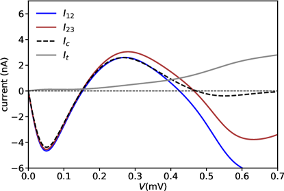
Figure 3: (color online). Bond current, chiral current and transport current versus bias. The triangle-up marker and triangle-down marker correspond to the clockwise and anticlockwise vertex current are schematically shown in Fig.1 in the main text. The other parameters are $\Delta=0.025$, $t=0.25$, $T=0.05$, $\epsilon=-0.5$, $U=1.0$.

The comparison between chiral and bond current is shown in Fig. 3. The bond current $I_{13}$ is not depicted because of the Kirchhoff law $I_{13}=-I_{12}$. Under the restriction of the Kirchhoff’s law, the bond currents are favorable to have a unified magnitude and toroidal direction to minimize the coupling energy $H_{A}$. Therefore the bond current can be approximately regarded as the chiral current in small bias region, suggesting a nearly pure circling current with small leakage. At a higher voltage, the inter-dot current $I_{12}$ and $I_{23}$ splits and transport current increases rapidly, this is because the double occupation energy level and single particle energy level moves towards the Fermi energy of the electrodes.

V Magnetoelectric effect

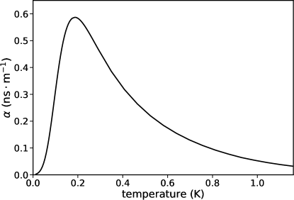
Figure 4: Magnetoelectric susceptibility of the TTQD as a function of temperature. The other parameters are the same as those used in Fig. 1 in the main text.

References

Taguchi et al. [2001]Y. Taguchi, Y. Oohara,
H. Yoshizawa, N. Nagaosa, and Y. Tokura, Science 291, 2573
(2001).
Noiri et al. [2017]A. Noiri, K. Kawasaki,
T. Otsuka, T. Nakajima, J. Yoneda, S. Amaha, M. R. Delbecq, K. Takeda, G. Allison,
A. Ludwig, A. D. Wieck, and S. Tarucha, Semicond. Sci. Technol. 32, 084004 (2017).
Hong et al. [2018]C. Hong, G. Yoo, J. Park, M.-K. Cho, Y. Chung, H.-S. Sim, D. Kim, H. Choi, V. Umansky, and D. Mahalu, Phys.
Rev. B 97, 241115(R)
(2018).
Woo et al. [2016]S. Woo, K. Litzius,
B. Krüger, M.-Y. Im, L. Caretta, K. Richter, M. Mann, A. Krone, R. M. Reeve,
M. Weigand, et al., Nat. Mater. 15, 501 (2016).
Landau et al. [2013]L. D. Landau, J. Bell,
M. Kearsley, L. Pitaevskii, E. Lifshitz, and J. Sykes, Electrodynamics of continuous media, Vol. 8 (elsevier, 2013).
Dzyaloshinskii [1960]I. E. Dzyaloshinskii, Sov. Phys. JETP 10, 628
(1960).