Online Hashing with Efficient Updating of Binary Codes
Abstract
Online hashing methods are efficient in learning the hash functions from the streaming data. However, when the hash functions change, the binary codes for the database have to be recomputed to guarantee the retrieval accuracy. Recomputing the binary codes by accumulating the whole database brings a timeliness challenge to the online retrieval process. In this paper, we propose a novel online hashing framework to update the binary codes efficiently without accumulating the whole database. In our framework, the hash functions are fixed and the projection functions are introduced to learn online from the streaming data. Therefore, inefficient updating of the binary codes by accumulating the whole database can be transformed to efficient updating of the binary codes by projecting the binary codes into another binary space. The queries and the binary code database are projected asymmetrically to further improve the retrieval accuracy. The experiments on two multi-label image databases demonstrate the effectiveness and the efficiency of our method for multi-label image retrieval.
Introduction
With the explosive growth of the image data, finding the nearest neighbors to a query becomes a fundamental research problem in many computer vision applications (?). Due to the efficiency in terms of space and time, hashing methods are widely used for nearest neighbor search, where the high-dimensional data are mapped to the binary codes (?; ?; ?).
The hashing methods (?; ?; ?) have achieved the promising performance. By learning the hash functions according to the data distribution and the label information, the hashing methods can map the high-dimensional data to the compact binary codes, and the similarity between the data can be preserved by the Hamming distance between the binary codes. However, these methods are batch-based hashing methods, which need to load the whole database into RAM to learn the hash functions. Due to the limited memory space, the deep hashing methods (?; ?) adopt minibatch-based stochastic optimization which requires multiple passes over a given database to learn the hash functions. However, they still have poor scalability for the large-scale application. Since the image data keep growing in the real application, to adapt to the change of the data, the hash functions need to be re-trained by accumulating the whole database when new data appear, which is time-consuming.
 |
 |
| (a) Updating hash functions | (b) Updating projection functions |
Online hashing methods (?; ?; ?; ?; ?; ?; ?; ?) are recently proposed to employ online learning techniques on the streaming data. By learning the hash functions from the streaming data, online hashing methods can adapt to the data variations with low computational complexity. According to their application scenarios, the online hashing methods can be categorized as single image modality retrieval (?; ?; ?) and cross-modal retrieval (?). In this paper, we focus on the single image modality retrieval.
Online Sketch Hashing (OSH) (?) maintains a data sketch to preserve the properties of the streaming data and learns the hash functions from the data sketch. But it is an online unsupervised hashing method which cannot use the label information to improve the retrieval accuracy. To take advantage of the label information, following the Passive-Aggressive algorithm (?), Online Kernel-based Hashing (OKH) (?) defines a structured similarity loss function and updates the hash functions according to the loss function when receiving a new pair of the data and their similarity label. Mutual Information Hashing (MIH) (?) uses the mutual information as the objective function and updates the hash functions according to the objective function with each incoming data point and its corresponding class label. Online Supervised Hashing (OSupH) (?) generates error correcting output codes according to the label information and uses these codes to guide the learning process of the hash functions from the streaming data. Balanced Similarity for Online Discrete Hashing (BSODH) (?) preserves the correlation between the streaming data and the existing database via an asymmetric graph regularization and updates the hash functions with this correlation.
Although some progress has been made, the online hashing methods discussed above simply focus on modeling the hash functions to be updated efficiently. They ignore the problem that the binary codes for the indexed data have to be updated to guarantee the retrieval accuracy whenever the hash functions change, and updating the binary codes frequently by accumulating the ever-increasing database inevitably blocks the timeliness of the online retrieval process. Though the previous work, , MIH (?) tries to solve this problem by introducing a trigger update module to reduce the frequency of recomputing the binary codes. However, the calculation in the trigger update module is time-consuming. Cross-Modal Hashing (OCMH) (?) also detects the inefficiency of accumulating the whole database to update the binary codes and improves the updating efficiency by representing the binary codes with the permanent latent sharing codes and the dynamic transfer matrix. But this method is designed for the cross-modal retrieval application, and cannot be directly used for single image modality retrieval.
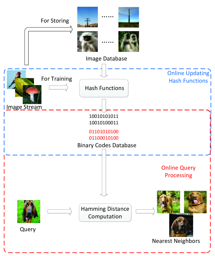
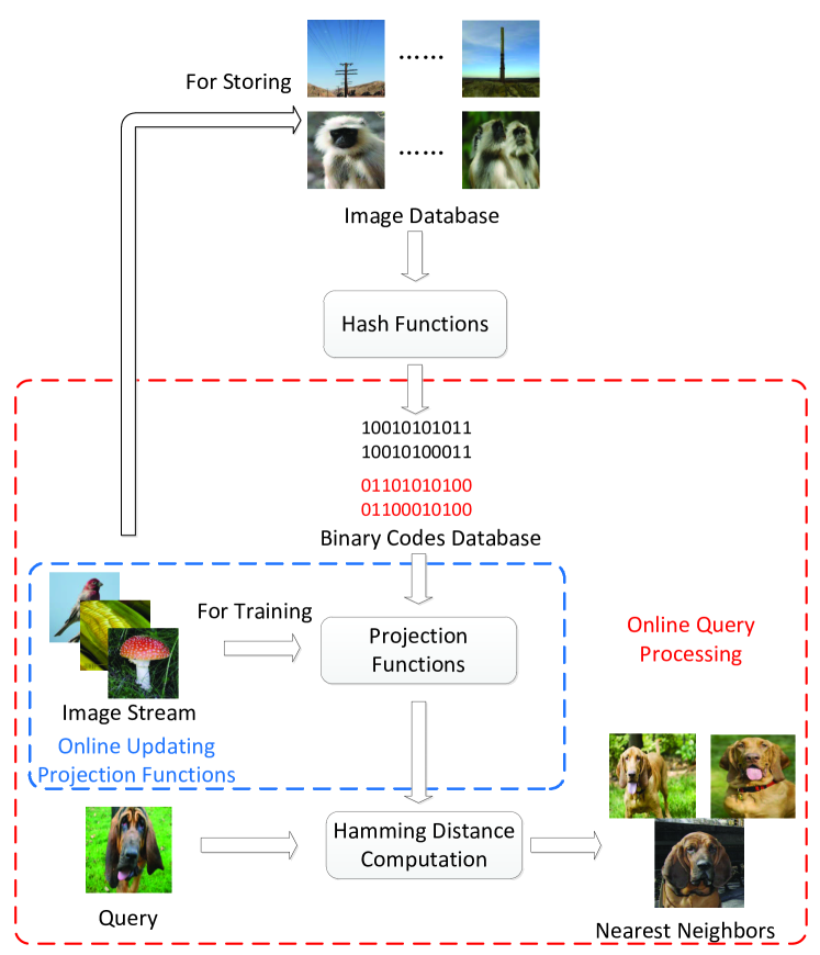
In this paper, we propose a novel online hashing framework to update the binary codes without accumulating the whole database. Different from the above online hashing methods that learn the hash functions from the streaming data, in our framework, the hash functions are fixed and the projection functions are introduced to learn from the streaming data. Hence, inefficient updating of the binary codes by accumulating the whole database can be transformed to efficient updating of the binary codes by projecting the binary codes into another binary space. The comparison of our framework against the current online hashing methods is shown in Fig. 1. For the current online hashing methods, they update the hash functions from the streaming data. In contrast, in our framework, the hash functions are fixed, and the projection functions are updated from the streaming data.
To sum up, our contribution in this paper is three fold:
-
•
By introducing the projection functions, a novel online hashing framework is proposed to update the binary codes without accumulating the whole database.
-
•
Different from most online hashing methods using the single-label information to learn the hash functions, our framework takes advantage of the multi-label information to learn the projection functions.
-
•
To further improve the retrieval accuracy, the projection functions for the queries and the binary code database are learnt in an asymmetric way.
Online Hashing with Efficient Updating
Hash Function
Given a set of image features , where and is the dimensionality of the feature vector, hashing methods aim to map to a -bit binary code . For a pair of data points and , the hamming distance between them is calculated as
| (1) |
where is an xor operation.
Following (?; ?), we adopt the linear projection-based hash functions. To encode a given data point into a -bit binary code, the hash function is defined as
| (2) |
where is a projection matrix and is a threshold vector.
Different from other online hashing methods that update the projection matrix , in our method, we fix and learn the projection functions to map the generated binary code into another binary space, which will be elaborated in the next subsection.
We use Iterative Quantization (PCA-ITQ) (?) to learn . PCA-ITQ is an unsupervised hashing method which can preserve the similarity between data effectively for both the seen and the unseen data. By setting the threshold value of as the negative mean of the data on the dimension and learning a projection matrix , PCA-ITQ can minimize the quantization error between the projected data and the corresponding binary codes. PCA-ITQ is traditionally a batch-based hashing method. Nevertheless, recent advance (?) shows that this hashing method can preserve the data similarity well by just using a few data points as the training data for learning the hash functions. Hence, we adopt PCA-ITQ to learn the hash functions in the initial stage. Following (?), we assume that at least data points have been provided in the initial stage, and the hash functions are learnt according to these data points.
Projection Function
Assume a stochastic environment in which data come sequentially along with the class label , where is the label space. For a pair of data points and , their corresponding binary codes are and , respectively. In our method, as the hash functions are fixed, to use the label information, each binary code is mapped to another binary code , which is defined as
| (3) |
where is a projection matrix.
Hence, the similarity between the data in our method is calculated as
| (4) |
Inspired by OKH (?) and OSupH (?) which generate the ideal binary code according to the supervised information to guide the updating of the hash functions, we generate the ideal binary code according to the class label to guide the updating of the projection functions.
Different from OKH and OSupH that consider about the single-label situation, our method considers about the multi-label situation, and generates the ideal binary code that contains the multi-label information. In the label space of classes, we use one-hot coding, and thus where the entry is 1 if the data point belongs to the class. It has been proved in (?) that Locality Sensitive Hashing (LSH) (?) can preserve the semantic similarity among label-based representation. If two labels are similar, the collision probability of the corresponding binary codes is greater than 0.5. Otherwise, the collision probability is less than 0.5. Hence, for a given data point and its label , the ideal binary code is
| (5) |
where is a random matrix of which each column is sampled from the normal Gaussian distribution .
The projection matrix is composed of projection vectors and each vector corresponds to one bit of the ideal binary code. Different from other online hashing methods (?; ?) that treat the bits collectively, we treat the bits independently. The value of each bit is 1 or -1, and the projection vectors are learnt independently.
Inspired by (?), we update the projection vectors from the streaming data in a Passive-Aggressive (PA) way. For notational simplicity, we use to denote the vector as each projection vector is learnt independently, and to denote the corresponding bit of the ideal binary code for the label of the data point . The loss function for each coming data point is defined as
| (6) |
where is the corresponding binary code of .
For brevity, we use to denote the loss for the data point. At first, is initialized with a random value. Then, for each round , we solve the following convex problem with soft margin:
| (7) |
where is the Euclidean norm and is the aggressiveness parameter that controls the trade-off between maintaining close to the previous parameter and minimizing the loss on the current loss .
When = 0, = satisfies Eqn.(7) directly. Otherwise, we define the Lagrangian as:
| (8) |
with and are Lagrange multipliers.
Let . We have
| (9) |
Let . We have
| (10) |
As , .
Plugging Eqn.(9) and (10) back in Eqn.(8), we obtain
| (11) |
As , . As , . Let . We have
| (12) |
Hence, the optimal is
| (13) |
where
| (14) |
Hence, when given a query , the similarity between the query and the binary code is calculated as
| (15) |
where is the corresponding binary code of the query .
Loss Bound
Based on the Lemma 1 in (?), we can obtain the following theorem.
Let (, ),,(, ) be a sequence of pair-wise examples with label for all . As before, Eqn.(6) denotes by , the instantaneous loss suffered by our method on round . Let be an arbitrary vector that , and define , as the loss suffered by . Then, for any vector , the number of prediction mistakes made by our method on this sequence of examples is bounded by
| (16) |
According to Eqn.(6), if our method makes a prediction mistake on round then . Therefore, according to Eqn.(14), we have
| (17) |
Let be the number of prediction mistakes made on the entire sequence. We have,
| (18) |
According to Eqn.(12), we know that
| (19) |
and
| (20) |
According to 1 in (?), we have
| (21) |
Plugging Eqn.(19) and (20) into Eqn.(21), we obtain
| (22) |
Combining Eqn.(18) with Eqn.(22), we obtain
| (23) |
Multiplying both sides of the above by , we have
| (24) |
Asymmetric Projection
In (?), it shows that treating the query points and the database points asymmetrically can improve the search accuracy of the binary codes. Hence, we treat the query points and the database points in an asymmetric way by learning different projection functions. Instead of using the projection matrix after hashing the query into a binary code, we learn a projection matrix that can be directly applied on the original query feature . Hence, the similarity between the query and the binary code is calculated as
| (25) |
where is the corresponding binary code of .
The projection matrix is also composed of projection vectors and each vector corresponds to one bit of the ideal binary code. For notational simplicity, we use to denote the vector . The loss function of for each coming data point is defined as:
| (26) |
For brevity, we use to denote the loss for the data point. Then, for each round , we solve the following convex problem with soft margin:
| (27) |
Therefore, the optimal is
| (28) |
where
| (29) |
The derivation of Eqn.(28) is similar to the derivation of Eqn.(13), and is provided in Appendix A of the supplementary file.
By assuming , the prediction mistake of our method on the queries is bounded according to .
Let (, ),,(, ) be a sequence of pair-wise examples with label for all . As before, Eqn.(26) in the manuscript denotes by , the instantaneous loss suffered by our algorithm on round . Let be an arbitrary vector that , and define , as the loss suffered by . Then, by assuming , for any vector , the number of prediction mistakes made by our method on this sequence of examples is bounded by
| (30) |
The proof of is provided in Appendix B of the supplementary file.
As our method can update the binary codes efficiently, our method is called Online Hashing with Efficient Updating (OHWEU). The pseudo-code of our method is shown in Algorithm 1.
Experiments
Datasets
We compare our method on two commomly-used multi-label image datasets, MS-COCO and NUS-WIDE.
(a).MS-COCO dataset (?). The MS-COCO dataset is a multi-label dataset consisting of training images and 40,504 validation images. Each image is labeled by some of the 80 concepts. We obtain 122,218 images after we filter the images that do not contain any concept label and combine the training images with the validation images. Each images is represented by a 4096-D feature extracted from the fc7 layer of a VGG-16 network (?) pretrained on ImageNet (?). We randomly take 4000 images as the queries, and the rest for training and searching.
(b). NUS-WIDE dataset (?). The NUS-WIDE dataset is also a multi-label dataset, which consists of 269,648 web images associated with tags. Following (?), we only select the images that belong to the 21 most frequent concepts. Hence, we have 195,834 images. Each images is represented by a 4096-D feature extracted from the fc7 layer of a VGG-16 network (?) pretrained on ImageNet. We randomly take 2000 images as the queries, and the rest for training and searching.
The experiments are run on a computer with CPU I7, 24-GB memory. Mean Average Precision (mAP) is used to measure the performance of the online hashing methods. If two images share at least one common label, they are defined as a groundtruth neighbor. The results are averaged by repeating the experiments 3 times.
 |
 |
| (a) MS-COCO | (b) NUS-WIDE |
 |
 |
 |
 |
| (a) 32 bits | (b) 64 bits | (c) 96 bits | (d) 128 bits |
Comparison of Accuracy
We compare our method with BSODH (?), MIH (?), OSupH (?), OKH (?), OSH (?), The key parameters in each compared method are set as the ones recommended in the corresponding papers. In MIH, the reservoir size is set to 200 as the reservoir size is related to the training time cost of MIH. As OKH does, we have = 300 data points to train the hash functions in the initial stage.
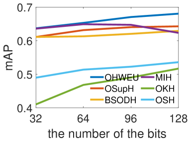
Fig. 2 shows the mAP results from 32 bits to 128 bits. On MS-COCO, our method outperforms other online hashing methods. And OSupH is the second best online hashing method. On NUS-WIDE, our method is still the best method among the online hashing methods. From 32 bits to 96 bits, MIH is the second best online hashing methods, while OSupH is the second best online hashing method for 128 bits.
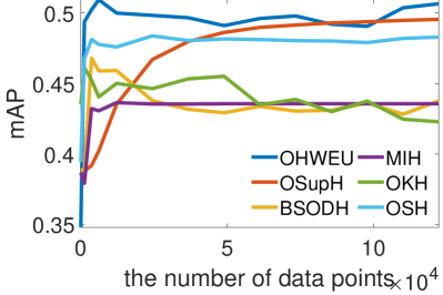
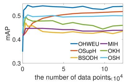
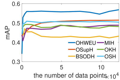
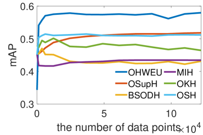
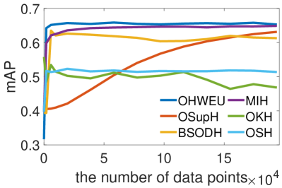
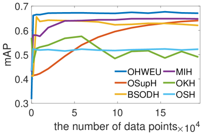
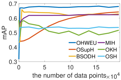
Fig. 3 shows the mAP performance of different online hashing methods with the training data increasing from 32 bits to 128 bits on MS-COCO. According to the results, we can see that our method outperforms other online hashing methods after taking only a few training data for training. And our method has a stable generalization ability as our method can achieve the satisfactory performance with only a few training data.
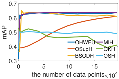
Fig. 4 shows the mAP performance of different online hashing methods with the training data increasing from 32 bits to 128 bits on NUS-WIDE. For 32 bits, the curves of our method, MIH, and BSODH are very close, our method has a close performance to MIH and BSODH. From 64 bits to 128 bits, our method obviously outperforms MIH, BSODH, and other online hashing methods.
 |
 |
 |
 |
| (a) 32 bits | (b) 64 bits | (c) 96 bits | (d) 128 bits |
 |
 |
 |
 |
| (a) 32 bits | (b) 64 bits | (c) 96 bits | (d) 128 bits |
Comparison of Efficiency
Table 1 and 2 show the training time of different online hashing methods on NUS-WIDE and MS-COCO, respectively. From the results, we can see that our method is faster than other online hashing methods. OSupH and MIH are much slower than other hashing methods. In addition to learning the hash functions, MIH introduces a trigger update module to determine whether to update the binary codes by evaluating the performance of the hash functions on the reservoir sample, and the calculation in the trigger update module is time-consuming. OSupH adopts the online boosting algorithm and needs to consider the hash functions on the previous bits when learning one hash function, which is inefficient, especially for the long bits.
| 32 bits | 64 bits | 96 bits | 128 bits | |
|---|---|---|---|---|
| OSH | 484.39 | 524.09 | 599.66 | 693.28 |
| OSupH | 2964.77 | 14146.94 | 33543.83 | 60548.74 |
| MIH | 17759.40 | 27008.53 | 40120.89 | 64800.35 |
| BSODH | 2116.42 | 2404.66 | 2881.74 | 3498.40 |
| 32 bits | 64 bits | 96 bits | 128 bits | |
|---|---|---|---|---|
| OSH | 335.28 | 387.80 | 485.61 | 606.08 |
| OSupH | 3650.17 | 12230.75 | 25880.18 | 53348.59 |
| MIH | 43091.97 | 60450.99 | 73379.56 | 80787.40 |
| BSODH | 3052.27 | 3251.55 | 3617.38 | 3786.90 |
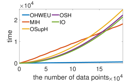
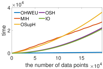
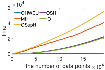
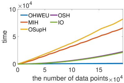
Following the setting in (?), we assume the data come in chunks. Each chunk is composed of 1000 data points. We simulate a situation that exchanges the data between the hard disk and RAM to compute the new binary codes, which is implemented by C++ code. It takes 3.97s to transfer 1000 4096-D data points from the hard disk to RAM averagely. Fig. 5 shows the accumulated time cost of different online hashing methods with the data samples increasing for different online hashing methods on NUS-WIDE from 32 bits to 128 bits. ’IO’ denotes the time cost of accumulating all the received data to update the binary codes. The experiments are run on a PC with Intel i7 3.4 GHz CPU, 24 GB memory.
According to the results in Fig. 5, our method has the lowest time cost among the online hashing methods, since our method has a low time cost for learning the projection functions and does not need to accumulate the whole database to update the binary codes. For OSupH, OSH, and IO, the accumulated time cost rises as an quadratic function of the number of data. Comparing OSH with IO, we can see that most of the time cost of OSH comes from transferring the data from the disk to RAM for the updating of the binary codes. MIH adopts the trigger update module to automatically determine when to recompute the binary codes, and its time cost is approximately linear to the data size. However, its time cost is still high as using the trigger update module to determine whether to update is time-consuming.
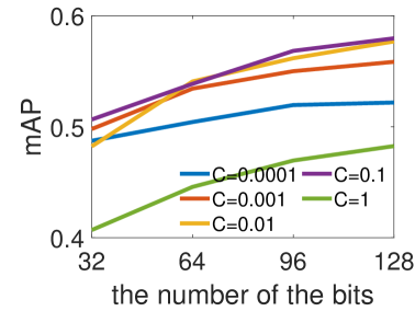
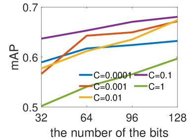
Parameter Analysis
As indicated in Eqn. (6), is used to control the trade-off between maintaining the projection vectors close to the previous ones and minimizing the current loss. We investigate the influence of the parameter . Fig. 6 shows our method with different on MS-COCO and NUS-WIDE. From the results, we can see that on both datasets, the performance of the proposed method becomes better when increases at first. However, when reaches some threshold, further increasing leads to the performance degradation. Based on the results, we set for MS-COCO and NUS-WIDE.
 |
 |
| (a) MS-COCO | (b) NUS-WIDE |
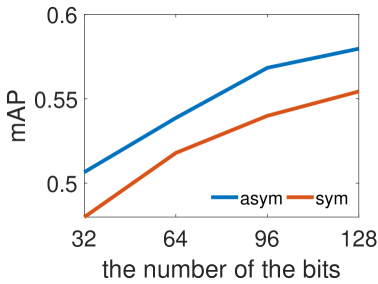
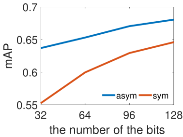
Fig. 7 shows the comparison of our method with different ways to process the queries and the binary code database. “sym” denotes that our method treats the queries and the binary code database symmetrically, and compares the query with the database points according to Eqn. (15). “asym” denotes that our method uses an asymmetric way and compares the query and the database points according to Eqn. (25). According to the results, “asym” outperforms “sym”, which shows that treating the query and the database asymmetrically can improve the search accuracy.
 |
 |
| (a) MS-COCO | (b) NUS-WIDE |
Conclusions
In this paper, we propose a new online hashing framework to update the binary codes efficiently without accumulating the whole database. Different from the widely-used online hashing methods, in our framework, the hash functions are fixed and the projection functions are updated from the streaming data to project the binary codes into another binary space. Hence, the binary codes can be updated efficiently. The experiments show that our method can achieve better retrieval accuracy with lower time cost compared to other online hashing methods for multi-label image retrieval.
Acknowledgements
This work is supported by Shenzhen Municipal Development and Reform Commission (Disciplinary Development Program for Data Science and Intelligent Computing), Key-Area Research and Development Program of Guangdong Province (2019B010137001), NSFC-Shenzhen Robot Jointed Founding (U1613215).
References
- [Andoni and Indyk 2006] Andoni, A., and Indyk, P. 2006. Near-optimal hashing algorithms for approximate nearest neighbor in high dimensions. In 47th Annual IEEE Symposium on Foundations of Computer Science, 459–468.
- [Cakir and Sclaroff 2015] Cakir, F., and Sclaroff, S. 2015. Adaptive hashing for fast similarity search. In Proceedings of the IEEE International Conference on Computer Vision, 1044–1052.
- [Cakir, Bargal, and Sclaroff 2017] Cakir, F.; Bargal, S. A.; and Sclaroff, S. 2017. Online supervised hashing. Computer Vision and Image Understanding 156:162–173.
- [Cakir et al. 2017] Cakir, F.; He, K.; Bargal, S. A.; and Sclaroff, S. 2017. Mihash: Online hashing with mutual information. In Proceedings of the IEEE International Conference on Computer Vision, 437–445.
- [Chua et al. ] Chua, T.-S.; Tang, J.; Hong, R.; Li, H.; Luo, Z.; and Zheng, Y. Nus-wide: A real-world web image database from national university of singapore. In Proceedings of the ACM International Conference on Image and Video Retrieval, 48:1–48:9.
- [Crammer et al. 2006] Crammer, K.; Dekel, O.; Keshet, J.; Shalev-Shwartz, S.; and Singer, Y. 2006. Online passive-aggressive algorithms. Journal of Machine Learning Research 7(Mar):551–585.
- [Deng et al. 2009] Deng, J.; Dong, W.; Socher, R.; Li, L.-J.; Li, K.; and Fei-Fei, L. 2009. ImageNet: A Large-Scale Hierarchical Image Database. In Proceedings of the IEEE Conference on Computer Vision and Pattern Recognition, 1–8.
- [Ding et al. 2018] Ding, K.; Huo, C.; Fan, B.; Xiang, S.; and Pan, C. 2018. In defense of locality-sensitive hashing. IEEE Trans. on Neural Networks and Learning Systems 29(1):87–103.
- [Ghasedi Dizaji et al. 2018] Ghasedi Dizaji, K.; Zheng, F.; Sadoughi, N.; Yang, Y.; Deng, C.; and Huang, H. 2018. Unsupervised deep generative adversarial hashing network. In Proceedings of the IEEE Conference on Computer Vision and Pattern Recognition.
- [Gong et al. 2013] Gong, Y.; Lazebnik, S.; Gordo, A.; and Perronnin, F. 2013. Iterative quantization: A procrustean approach to learning binary codes for large-scale image retrieval. IEEE Trans. on Pattern Anal. and Mach. Intell. 35(12):2916–2929.
- [He, Wang, and Cheng 2019] He, X.; Wang, P.; and Cheng, J. 2019. K-nearest neighbors hashing. In Proceedings of the IEEE Conference on Computer Vision and Pattern Recognition, 2839–2848.
- [Huang, Yang, and Zheng 2018] Huang, L.; Yang, Q.; and Zheng, W. 2018. Online hashing. IEEE Trans. on Neural Networks and Learning Systems 29(6):2309–2322.
- [Kang, Li, and Zhou 2016] Kang, W.-C.; Li, W.-J.; and Zhou, Z.-H. 2016. Column sampling based discrete supervised hashing. In Association for the Advancement of Artificial Intelligence, 1230–1236.
- [Leng et al. 2015] Leng, C.; Wu, J.; Cheng, J.; Bai, X.; and Lu, H. 2015. Online sketching hashing. In Proceedings of the IEEE Conference on Computer Vision and Pattern Recognition, 2503–2511.
- [Li et al. 2019] Li, C.; Deng, C.; Wang, L.; Xie, D.; and Liu, X. 2019. Coupled cyclegan: Unsupervised hashing network for cross-modal retrieval. In AAAI Conference on Artificial Intelligence, 176–183.
- [Li, Liu, and Huang 2018] Li, Y.; Liu, W.; and Huang, J. 2018. Sub-selective quantization for learning binary codes in large-scale image search. IEEE Trans. on Pattern Anal. and Mach. Intell. 40(6):1526–1532.
- [Lin et al. 2014] Lin, T.-Y.; Maire, M.; Belongie, S.; Hays, J.; Perona, P.; Ramanan, D.; Dollár, P.; and Zitnick, C. L. 2014. Microsoft coco: Common objects in context. In Fleet, D.; Pajdla, T.; Schiele, B.; and Tuytelaars, T., eds., Proceedings of the European Conference on Computer Vision, 740–755.
- [Lin et al. 2018] Lin, M.; Ji, R.; Liu, H.; and Wu, Y. 2018. Supervised online hashing via hadamard codebook learning. In Proceedings of the ACM International Conference on Multimedia, 1635–1643.
- [Lin et al. 2019] Lin, M.; Ji, R.; Liu, H.; Sun, X.; Wu, Y.; and Wu, Y. 2019. Towards optimal discrete online hashing with balanced similarity. In Association for the Advancement of Artificial Intelligence, 8722–8729.
- [Liu et al. 2017] Liu, L.; Lin, Z.; Shao, L.; Shen, F.; Ding, G.; and Han, J. 2017. Sequential discrete hashing for scalable cross-modality similarity retrieval. IEEE Trans. on Image Processing 26(1):107–118.
- [Lu, Liong, and Zhou 2017] Lu, J.; Liong, V. E.; and Zhou, J. 2017. Deep hashing for scalable image search. IEEE Trans. on Image Processing 26(5):2352–2367.
- [Neyshabur et al. 2013] Neyshabur, B.; Srebro, N.; Salakhutdinov, R. R.; Makarychev, Y.; and Yadollahpour, P. 2013. The power of asymmetry in binary hashing. In Burges, C. J. C.; Bottou, L.; Welling, M.; Ghahramani, Z.; and Weinberger, K. Q., eds., Advances in Neural Information Processing Systems. 2823–2831.
- [Simonyan and Zisserman 2014] Simonyan, K., and Zisserman, A. 2014. Very deep convolutional networks for large-scale image recognition. CoRR abs/1409.1556.
- [Song et al. 2018] Song, J.; He, T.; Gao, L.; Xu, X.; Hanjalic, A.; and Shen, H. T. 2018. Binary generative adversarial networks for image retrieval. In AAAI Conference on Artificial Intelligence, 394–401.
- [Wang et al. 2018] Wang, J.; Zhang, T.; Song, J.; Sebe, N.; and Shen, H. T. 2018. A survey on learning to hash. IEEE Trans. on Pattern Anal. and Mach. Intell. 40(4):769–790.
- [Wang, Kumar, and Chang 2012] Wang, J.; Kumar, S.; and Chang, S.-F. 2012. Semi-supervised hashing for large-scale search. IEEE Trans. on Pattern Anal. and Mach. Intell. 34(12):2393–2406.
- [Xie et al. 2017] Xie, L.; Shen, J.; Han, J.; Zhu, L.; and Shao, L. 2017. Dynamic multi-view hashing for online image retrieval. In Proceedings of the International Joint Conference on Artificial Intelligence, 3133–3139.
- [Xie, Shen, and Zhu 2016] Xie, L.; Shen, J.; and Zhu, L. 2016. Online cross-modal hashing for web image retrieval. In Association for the Advancement of Artificial Intelligence, 294–300.
Appendix A. Derivation of
The projection matrix is composed of projection vectors and each vector corresponds to one bit of the ideal binary code. For notational simplicity, we use to denote the vector . The loss function of for each coming data point is defined as:
| (31) |
For brevity, we use to denote the loss for the data point. Then, for each round , we solve the following convex problem with soft margin:
| (32) |
When = 0, = satisfies Eqn.(2) directly. Otherwise, we define the Lagrangian as:
| (33) |
with and are Lagrange multipliers.
Let . We have
| (34) |
Let . We have
| (35) |
As , .
Plugging Eqn.(4) and (5) back in Eqn.(3), we obtain
| (36) |
As , . Let . We have
| (37) |
Hence, the optimal is
| (38) |
where
| (39) |
Appendix B. Proof of
Let (, ),,(, ) be a sequence of pair-wise examples with label for all . As before, Eqn.(26) in the manuscript denotes by , the instantaneous loss suffered by our algorithm on round . Let be an arbitrary vector that , and define , as the loss suffered by . Then, by assuming , for any vector , the number of prediction mistakes made by our method on this sequence of examples is bounded by
| (40) |
As , by assuming , we have
According to the definition of the loss function, if our method makes a prediction mistake on round then . Therefore, we have
| (41) |
Let be the number of prediction mistakes made on the entire sequence. We have,
| (42) |
Since , we know that
| (43) |
and
| (44) |
According to 1 in (?), we have
| (45) |
Plugging Eqn.(13) and (14) into Eqn.(15), we obtain
| (46) |
Combining Eqn.(12) with Eqn.(16), we obtain
| (47) |
Multiplying both sides of the above by , we have
| (48) |