Gravitational Lens System PS J0147+4630 (Andromeda’s Parachute): Main Lensing Galaxy and Optical Variability of the Quasar Images

Abstract

Because follow–up observations of quadruple gravitational lens systems are of extraordinary importance for astrophysics and cosmology, we present single–epoch optical spectra and $r$–band light curves of PS J0147+4630. This recently discovered system mainly consists of four images ABCD of a background quasar around a foreground galaxy G that acts as a gravitational lens. First, we use long–slit spectroscopic data in the Gemini Observatory Archive and a multi–component fitting to accurately resolve the spectra of A, D, and G. The spectral profile of G resembles that of an early–type galaxy at a redshift of 0.678 $\pm$ 0.001, which is about 20% higher than the previous estimate. Additionally, the stellar velocity dispersion is measured to $\sim$5% precision. Second, our early $r$–band monitoring with the Liverpool Telescope leads to accurate light curves of the four quasar images. Adopting time delays predicted by the lens model, the new lens redshift, and a standard cosmology, we report the detection of microlensing variations in C and D as large as $\sim$0.1 mag on timescales of a few hundred days. We also estimate an actual delay between A and B of a few days (B is leading), which demonstrates the big potential of optical monitoring campaigns of PS J0147+4630.

1 Introduction

Optical light curves of the four images of a quadruple gravitationally lensed quasar (quad) have a great potential to reveal physical properties of the lensed quasar, the main lensing galaxy, and the Universe as a whole. Thus, monitoring campaigns of QSO 2237+0305 (catalog ) (Einstein Cross; Woźniak et al., 2000; Alcalde et al., 2002; Eigenbrod et al., 2008a) have proved to be invaluable tools for unveiling the structure of the quasar accretion disk and the composition of the lensing galaxy (e.g., Shalyapin et al., 2002; Kochanek, 2004; Eigenbrod et al., 2008b). Most recently, light curves of other quads also led to important astrophysical results, e.g., an estimate of the accretion disk size in HE 0435$-$1223 (catalog ) and WFI 2033$-$4723 (catalog ) using microlensing–induced variations (Fian et al., 2018; Morgan et al., 2018), and a robust measurement of the Hubble constant $H_{0}$ from the time delays of HE 0435$-$1223 (catalog ), RXJ1131$-$1231 (catalog ), and B1608+656 (catalog ) (assuming a flat $\Lambda$CDM cosmology with free energy density $\Omega_{\Lambda}$; Bonvin et al., 2017). For a given quad, in addition to accurate time delays, the redshift and stellar velocity dispersion of the main lensing galaxy (and the properties of the lens environment) are required to obtain strong constraints on cosmological parameters (e.g., Suyu et al., 2017).

Berghea et al. (2017) reported the serendipitous discovery of the bright quad PS J0147+4630 (catalog ) using multiband frames from the Panoramic Survey Telescope and Rapid Response System (Pan-STARRS; Chambers et al., 2016). The four images of this first Pan-STARRS lensed quasar are not arranged like a cross, but rather resembling the shape of an open parachute (Andromeda’s Parachute). An arc–like structure contains the three brightest images (A, B and C; $r\sim$ 16$-$16.5 mag), while the fourth component D ($r\sim$ 18 mag) is located about 3″ from such arc. The main lensing galaxy (G; $r\sim$ 20 mag) and D are only $\sim$1″ apart. Additionally, spectroscopic observations indicated the broad absorption line (BAL) nature of the quasar, which has a redshift of 2.341 $\pm$ 0.001 (Lee, 2017) and is absorbed by several intervening metal systems (Rubin et al., 2018). From long–slit optical spectroscopy with GMOS on the 8.1 m Gemini North Telescope (GNT), Lee (2018) also found a lens redshift $z_{\rm{G}}$ = 0.5716 $\pm$ 0.0004. These redshifts and Hubble Space Telescope ($HST$) imaging of the lens system allowed Shajib et al. (2019) to predict time delays between the quasar images for a flat $\Lambda$CDM cosmology with $H_{0}$ = 70 km s^-1 Mpc^-1 and $\Omega_{\Lambda}$ = 0.7 ($\Omega_{m}$ = 0.3).

The Gravitational LENses and DArk MAtter (GLENDAMA) project is conducting optical observations of a sample of ten lensed quasars with bright images ($r<$ 20 mag) at $1<z<3$ (Gil-Merino et al., 2018). This representative sample includes the quad PS J0147+4630 (catalog ), which is being monitored with the 2.0 m Liverpool Telescope (LT) since 2017 August. In Section 2, we reanalyse the GNT–GMOS data of PS J0147+4630 (catalog ) to accurately extract spectra for the three close sources within the slit (A, D and G). We then focus on the new spectrum of G, measuring its redshift and the stellar velocity dispersion. Implications of this data reanalysis are also discussed in Section 2. In Section 3, we present LT $r$–band light curves of the four images of PS J0147+4630 (catalog ) spanning two complete observing seasons from 2017 to 2019, and show the potential of optical monitoring programmes of this quad. We summarize the paper in Section 4.

2 Reanalysis of the GNT–GMOS spectroscopy: main lensing galaxy

Lee (2018) obtained GNT–GMOS spectroscopic data of PS J0147+4630 (catalog ) on 2017 September 2, consisting of 4$\times$1200 s long–slit exposures (B600 grating) taken under subarcsecond seeing conditions. The 0$\farcs$5–width slit with a spatial pixel scale of 0$\farcs$1614 was oriented along the line joining A and D (and crossing G). We downloaded these publicly available observations to reanalyse them. Our aim was to accurately resolve the individual spectra of the three sources in the crowded region through a well–tested state–of–the–art technique (see below). Before doing the extraction of spectra for A, D and G, usual data reductions were performed using the Gemini IRAF package. Regarding the wavelength range and dispersion, they were 4403$-$7605 Å and 1.02 Å pix^-1, respectively. We also inferred a resolving power of $\sim$2500 from the 2.24 Å width of the 5577 Å [O i] line in the night airglow.

We extracted the instrumental spectra of A, D and G by fitting three 1D Moffat profiles in the spatial direction for each wavelength bin (e.g., Sluse et al., 2007; Shalyapin & Goicoechea, 2017). For an extended source, an 1D point–spread function (PSF) model does not describe its total light. Therefore, since G was treated as a point–like object, we actually did not derive the overall spectrum of the galaxy. However, the flux ratio $A/G$ is $\sim$250, and the very faint galaxy does not play a relevant role when modeling the light distribution along the slit. This distribution is dominated by emission from A and D, so the critical issue is our ability to accurately account for the flux of both quasar images, minimising the contamination of G. We used $HST$ astrometry (Shajib et al., 2019) to set the positions of D and G with respect to A. In regard to the 1D PSF model, we checked that a skewed Moffat profile (Schönebeck et al., 2014) works better than the Gaussian or the symmetric Moffat one (see Appendix A; Moffat, 1969). Thus, we adopted a skewed Moffat function with $a_{6}$ = $a_{7}$ = 0, i.e., only the asymmetry parameter $a_{5}$ was considered (see Eq. 10 of Schönebeck et al., 2014). We also set the Moffat power–law index to an optimal value of 2. In a first fit to the multi–wavelength 1D flux distribution, the position (centroid) of A, the width and asymmetry of the Moffat function, and the amplitudes of the three components were allowed to vary at each wavelength. We then fitted A positions and Moffat structure parameters to smooth polynomial functions of the observed wavelength, fixing position–structure parameters to their polynomial values and leaving only the three amplitudes as free parameters in a second iteration.

Table 1: GNT–GMOS–B600 spectra of PS J0147+4630ADG.

$\lambda$	$F_{\lambda}$(A)	$eF_{\lambda}$(A)	$F_{\lambda}$(D)	$eF_{\lambda}$(D)	$F_{\lambda}$(G)	$eF_{\lambda}$(G)
4402.935	149.510	3.341	17.923	1.661	0.817	1.320
4403.956	149.636	3.344	17.938	1.663	0.818	1.321
4404.977	149.762	3.346	17.953	1.664	0.820	1.323
4405.998	149.889	3.349	17.968	1.666	0.822	1.324
4407.019	150.016	3.352	17.983	1.667	0.823	1.325

Note. — The spectrum of G is not properly calibrated, since fluxes are underestimated in a factor $\sim$5. Table 1 is published in its entirety in the machine-readable format. A portion is shown here for guidance regarding its form and content.

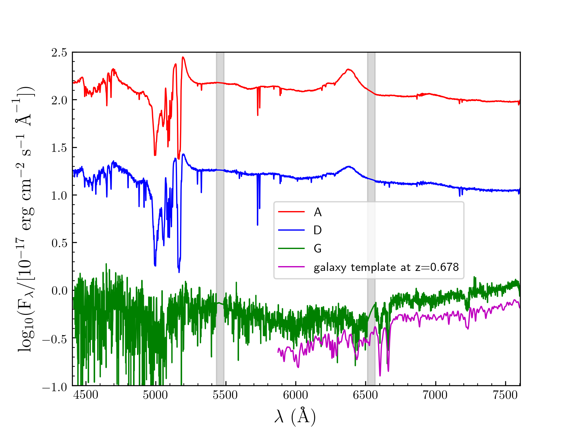
Figure 1: GNT–GMOS–B600 spectra of PS J0147+4630ADG in 2017 September. Flux is shown in a logarithmic scale to improve visibility, and grey highlighted bars are associated with gaps between the detectors. We note that the quasar spectra are reasonably well calibrated in flux, while the galaxy spectrum is not. The red–shifted ($z$ = 0.678) template of an early–type galaxy is also displayed for comparison purposes (see main text).

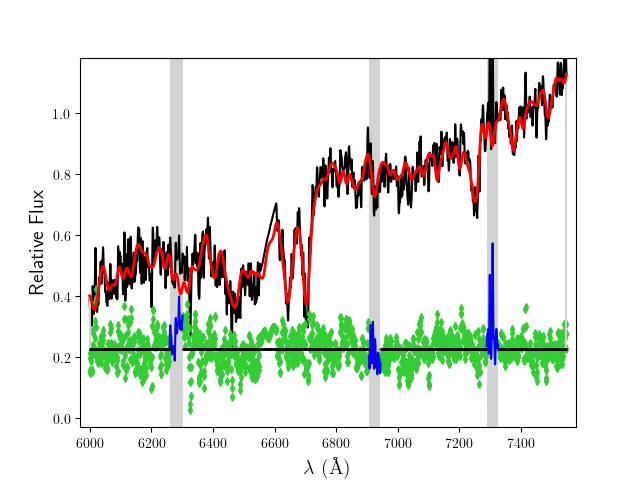
Figure 2: Stellar kinematics from the spectrum of the main lensing galaxy. The black line describes the observed spectrum, while the red line is the pPXF fit for the stellar component. Green symbols show the fit residuals, which are vertically shifted for clarity (see the horizontal line). The grey highlighted regions (residuals in blue) were excluded during the fitting process.

The four instrumental spectra of each source (one per exposure) were calibrated in flux and combined into a single spectral energy distribution. To carry out the flux calibrations, we used GNT–GMOS–B600 0$\farcs$5–width slit observations of the standard star EG 131 (Bessell, 1999) on 2017 September 4. Final spectra of A, D and G are included in Table 1 and plotted in Figure 1. A comprehensive analysys of the quasar spectra will be presented in a forthcoming paper. Here, we concentrate on the optical spectrum of the main lensing galaxy. The spectral slopes of G, as well as its Ca ii $H\&K$ doublet at about 6600&6660 Å and its G–band around 7225 Å, are in very good agreement with an early–type galaxy template at $z$ = 0.678 (see Figure 1). After doing an initial estimate for $z_{\rm{G}}$ from the observed absorption features, we accurately measured the lens redshift using the Penalized PiXel–Fitting (pPXF) package (Cappellari & Emsellem, 2004; Cappellari, 2017). This software compares the spectrum of G and stellar spectra, providing a correction to the initial value of $z_{\rm{G}}$ and measuring the stellar velocity dispersion. From the MILES Library of Stellar Spectra (Sánchez-Blázquez et al., 2006; Falcón-Barroso et al., 2011), we obtained $z_{\rm{G}}$ = 0.678 $\pm$ 0.001 and $\sigma_{\rm{G}}$ = 313 $\pm$ 14 km s^-1 (see Figure 2).

We note that our G spectrum and the redshifted template in Figure 1 are very similar, while the G spectrum in Fig. 2 of Lee (2018) does not resemble those of typical galaxies and seems to be heavily contaminated by quasar light. Thus, the previous identification of absorption lines of G is unreliable, and we adopt the new value of $z_{\rm{G}}$ as the lens redshift. For a flat $\Lambda$CDM cosmology with $H_{0}$ = 70 km s^-1 Mpc^-1 and $\Omega_{\Lambda}$ = 0.7, an 18.5% increase in the lens redshift, from 0.572 to 0.678, results in predicted time delays that are $\sim$27% longer than those in Table C1 of Shajib et al. (2019). These new delays are $\Delta t_{\rm{AB}}$ = $-$2.7, $\Delta t_{\rm{AC}}$ = $-$9, and $\Delta t_{\rm{AD}}$ = 245 days ($\Delta t_{\rm{XY}}=t_{\rm{Y}}-t_{\rm{X}}$). We also remark that the value of $z_{\rm{G}}$ plays a critical role in determining $H_{0}$ from measured time delays of the system. If we assume that $\Omega_{\Lambda}+\Omega_{m}$ = 1 and 0.6 $\leq\Omega_{\Lambda}\leq$ 0.8, then 1.266 $\leq H_{0}(z_{\rm{G}}=0.678)/H_{0}(z_{\rm{G}}=0.572)\leq$ 1.270.

3 Optical variability of the quasar images

3.1 LT–IO:O light curves

We monitored PS J0147+4630 (catalog ) with the LT from 2017 August to 2018 January and from 2018 July to 2019 February, i.e., during the first two visibility periods after its discovery. All observations were made using the Sloan $r$–band filter on the IO:O optical camera (pixel scale of 0$\farcs$30), and a single 120 s exposure was taken each observing night. Although we obtained 84 frames, six of them have poor quality and are not usable for doing photometry. Thus, in addition to basic instrumental reductions from the LT–IO:O pipeline, we used IRAF software (Tody, 1986, 1993) to remove cosmic rays and bad pixels from the remaining 78 frames. The central region of one of these usable frames is shown in Figure 3. This includes the four quasar images, as well as an isolated and unsaturated star at RA (J2000) = 26$\fdg$773246 and Dec. (J2000) = +46$\fdg$506670 ($r$ = 16.606 mag) that allows us to build up an empirical 2D PSF. A bright field star at RA (J2000) = 26$\fdg$746290 and Dec. (J2000) = +46$\fdg$504028 is also used as a control object having constant brightness $r$ = 15.421 mag (see the middle right side of Figure 3).

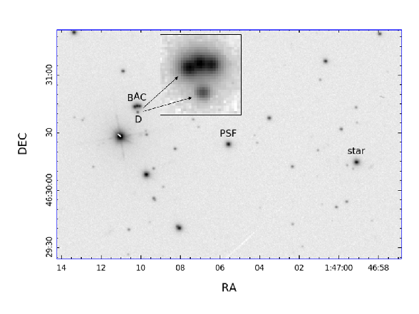
Figure 3: LT–IO:O subframe of PS J0147+4630 in the Sloan $r$ band. This subframe of size $3\arcmin\times 2\arcmin$ corresponds to the 120 s exposure in subarcsecond seeing on 2018 August 13. The field of view includes the quad with images ABCD (the strong lensing region is zoomed–in into the top sub–panel), the PSF star and the control star (see main text).

Table 2: Photometry of the lens system PS J0147+4630.

Civil Date	Epoch	FWHM	S/N	A	B	C	D	control star
170804	7970.051	1.06	454	15.961	16.190	16.632	18.203	15.426
170810	7976.081	0.95	334	15.953	16.198	16.622	18.211	15.421
170816	7982.116	0.75	402	15.956	16.190	16.623	18.223	15.408
170825	7991.048	0.95	395	15.960	16.208	16.634	18.237	15.414
170830	7996.225	1.27	466	15.955	16.191	16.637	18.237	15.416

Note. — Table 2 is published in its entirety in the machine-readable format. A portion is shown here for guidance regarding its form and content.

For each of the 78 fames, the brightness of A, B, C, D, and the control star were extracted through PSF fitting, using the IMFITFITS software (McLeod et al., 1998) and the PSF star located in the centre of the field of view in Figure 3. In the strong lensing region, ABCD and G were modeled as four point–like sources and a de Vaucouleurs profile convolved with the empirical 2D PSF, respectively. Our realistic overall model also incorporated several $HST$ constraints: positions of B, C, D, and G with respect to A, and structure parameters of G (Shajib et al., 2019). We applied the IMFITFITS code to the best frames to obtain the constant galaxy flux, and then to all frames (whatever their quality), fixing the galaxy flux and allowing the remaining parameters to vary, i.e., the absolute position of A and the four quasar fluxes (see Appendix B). In Table 2, we present values of the full–width at half–maximum (FWHM) of the seeing disk and the signal–to–noise ratio (S/N) for the PSF star, along with the $r$–band magnitudes of the quasar images and the control star.

To produce high–quality early light curves of PS J0147+4630 (catalog ), we selected the 70 observing epochs in Table 2 with FWHM $\leq$ 1$\farcs$6, and removed two additional epochs in which the B magnitude deviates significantly from adjacent values (2018 August 16 and 28). In Figure 4, we display our final light curves of the quasar images (filled symbols). From the data at these 68 epochs, we also estimated typical magnitude errors. For each image, relying on theoretical grounds, we calculated the standard deviation between magnitudes having time separations $\leq$ 4.5 days (i.e., using 31 pairs of consecutive magnitudes), and then divided it by the square root of 2. The resulting errors are 0.0053 (A), 0.0058 (B), 0.0093 (C), and 0.0154 (D) mag. These typical errors were multiplied by the relative S/N at each epoch, $\left<\rm{S/N}\right>/(\rm{S/N})_{\rm{epoch}}$, to obtain individual photometric uncertainties ($\left<\rm{S/N}\right>$ is the average S/N; Howell, 2006). We achieve $\sim$0.5–1.5% photometry over a period of about 1.6 years, which includes an unavoidable visibility gap of more than 5 months. The effective sampling rate (excluding the long gap) is $\sim$5 data per month.

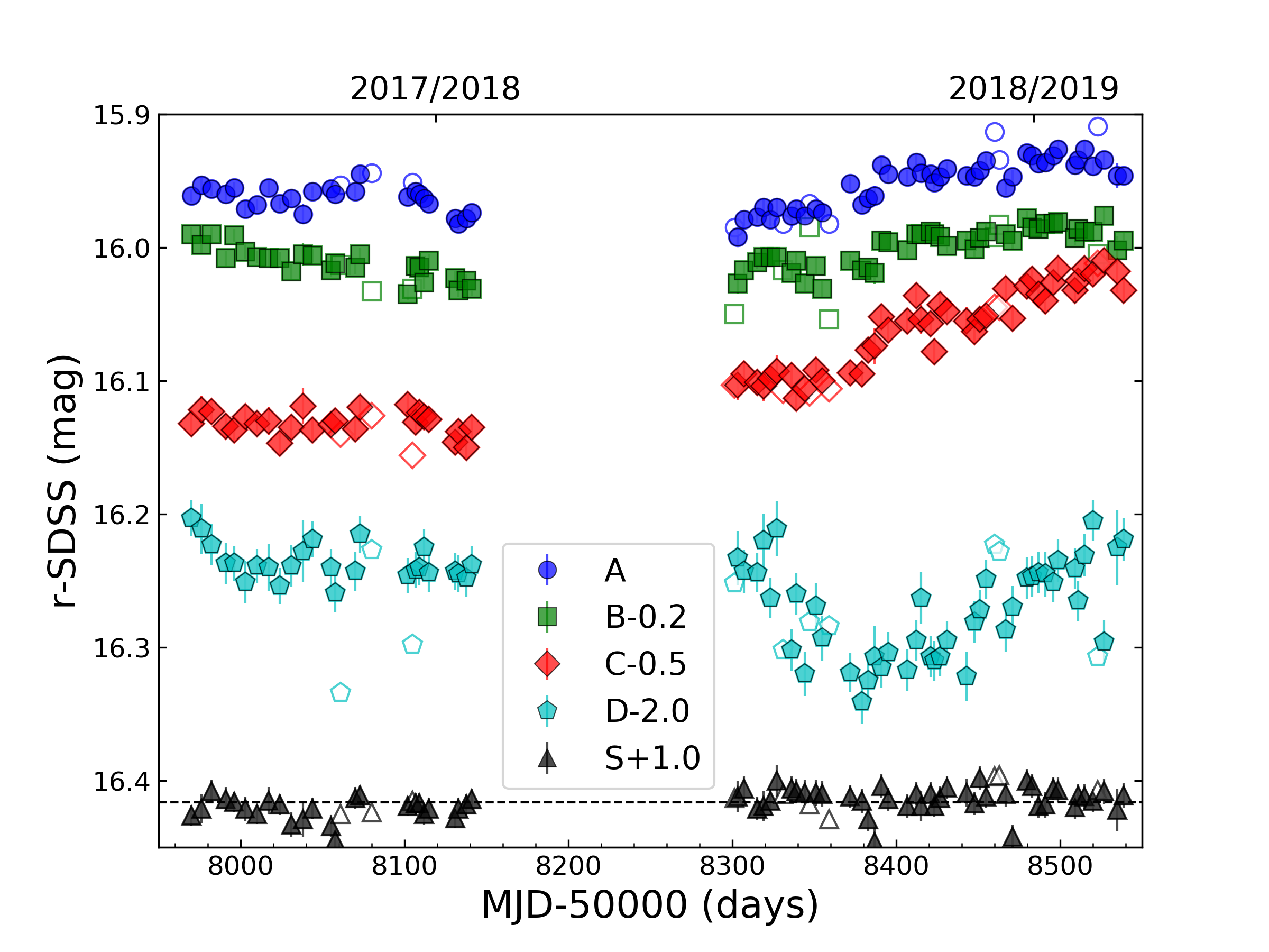
Figure 4: LT–IO:O $r$–band light curves of A, B, C, D, and the control star. The curves of B, C, D, and S (control star) are shifted by $-$0.2, $-$0.5, $-$2.0, and +1.0 mag, respectively, to facilitate comparison. The brightness records from all usable frames (see Table 2) are marked with filled and open symbols, while filled symbols trace the final light curves after removing 10 epochs (error bars of A, B, and C have sizes similar to those of symbols we use; see main text).

3.2 What can we learn from early light curves of the lensed quasar?

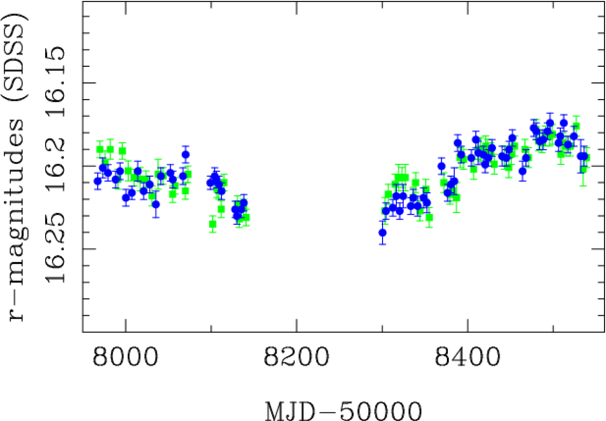
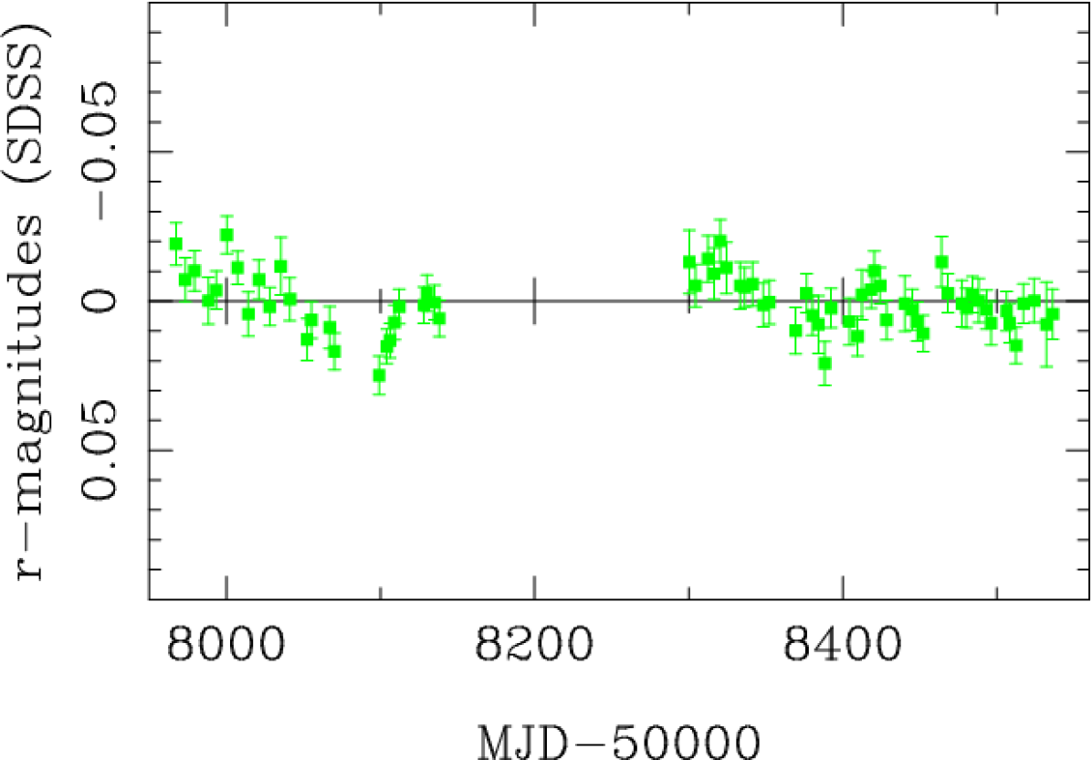
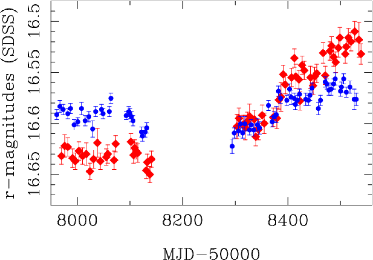
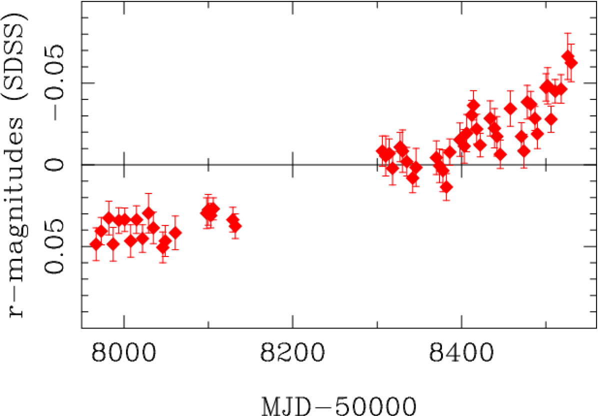
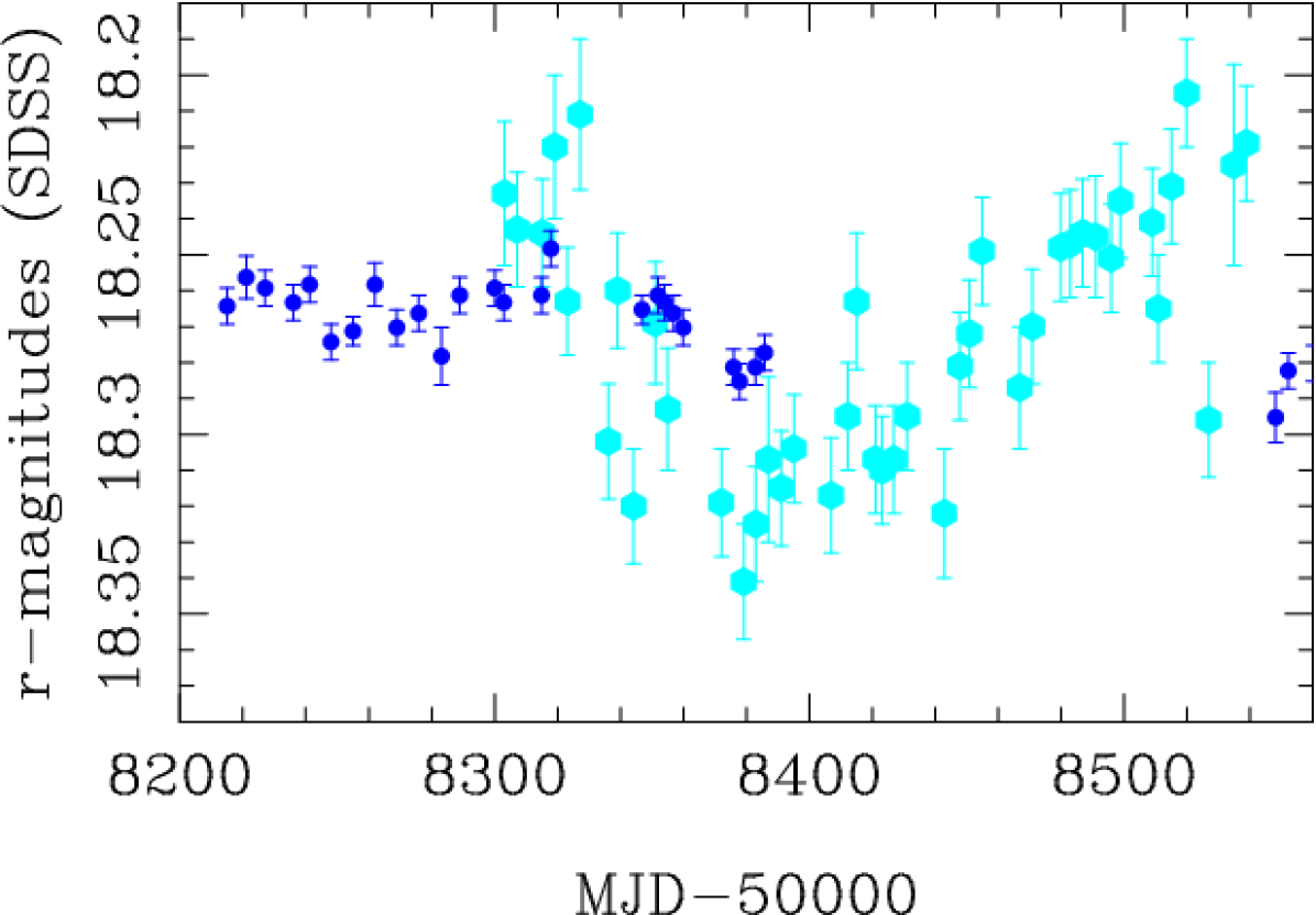
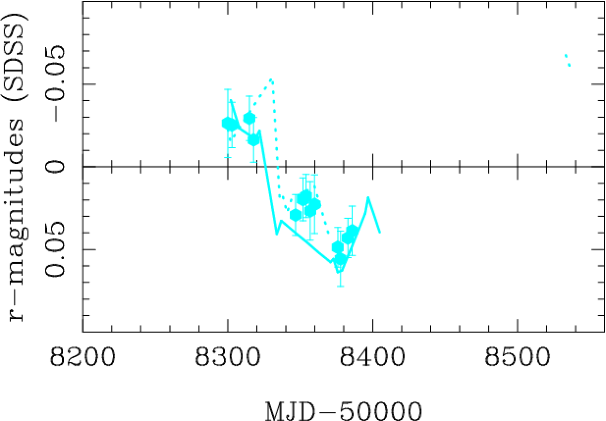
Figure 5: Combined and difference light curves in the $r$ band. The original B, C, and D brightness records are compared with magnitude– and time–shifted light curves of A in the top, middle, and bottom panels, respectively. Left: Combined curves. Right: Difference curves. In the bottom right panel, in addition to the curve derived through the expected delay for $H_{0}$ = 70 km s^-1 Mpc^-1 (filled symbols), we also show difference curves for two ”extreme” values of $H_{0}$ (e.g., Jackson, 2015): 65 (solid line) and 75 (dotted line) km s^-1 Mpc^-1. See main text for details.

The expected time delays in Section 2 and the early light curves of ABCD in Section 3.1 are useful tools to analyse the origin and properties of the quasar variability in the $r$ band. First, we obtained magnitude– and time–shifted light curves of image A as $m_{\rm{AY}}(t)=m_{\rm{A}}(t+\Delta t_{\rm{AY}})+\left<m_{\rm{Y}}-m_{\rm{A}}\right>$ for Y = B, C, and D; and later, each $\left[m_{\rm{AY}}(t),m_{\rm{Y}}(t)\right]$ combined pair was stacked together. These three combined light curves are shown in the left panels of Figure 5. Second, we computed difference light curves in a standard way, i.e., $m_{\rm{Y}}(t)-m_{\rm{AY}}(t)$ for Y = B, C, and D. For a given image Y, the dates in the magnitude– and time–shifted light curve of A, $m_{\rm{AY}}(t)$, were taken as reference epochs. Values of $m_{\rm{AY}}(t)$ were subtracted from averaged magnitudes of Y in bins with semiwidth $\alpha$ centred on the reference dates. We probed several reasonable values of $\alpha$, obtaining difference curves consistent with each other, and then setting $\alpha$ = 5 days (see the right panels of Figure 5). The AB comparison (top panels) indicates that both images exhibit almost parallel variations, so the difference light curve has a noisy behaviour around the zero level. Despite extrinsic (microlensing) variability can be present, it should consist of short timescale fluctuations with amplitudes $\leq$ 0.02 mag. However, the situation is quite different from the other two AC (middle panels) and AD (bottom panels) comparisons. In both cases, we detect significant microlensing variations. The difference light curves for C and D include $\sim$0.1 mag fluctuations over timescales from 100 to 400 days. Some other quads show similar levels of microlensing activity (e.g., Fian et al., 2018; Gil-Merino et al., 2018). We remark that microlensing signals in the D image rely on time delays $\Delta t_{\rm{AD}}$ predicted by the Shajib et al.’s mass model and plausible values of $H_{0}$. Despite the true value of $\Delta t_{\rm{AD}}$ might be slightly out of the delay range used in this paper, this would not produce noticeable changes with respect to the similar signals in the bottom right panel of Figure 5.

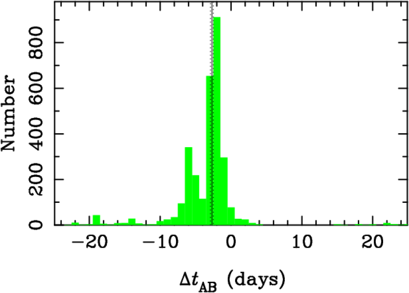
Figure 6: Delay histogram from 3000 pairs of simulated curves AB. The best solutions of $\Delta t_{\rm{AB}}$ are derived from a $D^{2}_{4,2}$ estimator ($\delta$ = 10 days) with two free parameters: time delay and magnitude offset. Predicted time delays for $H_{0}$ = 65$-$75 km s^-1 Mpc^-1 are shown by a vertical ”zipper”.

The LT–IO:O light curves of A and B over the two first monitoring seasons have similar shapes, providing evidence for intrinsic variability and enabling us to estimate $\Delta t_{\rm{AB}}$. As we only try to show the potential of monitoring campaigns of PS J0147+4630 (catalog ), instead of an exhaustive analysis from several cross–correlation techniques, we exclusively used the $D^{2}_{4,2}$ dispersion estimator (Pelt et al., 1996) to match both light curves. This method is simple and very popular, and it works in presence of short timescale microlensing (e.g., Goicoechea & Shalyapin, 2016). A comprehensive study of all time delays will be done when much more extended light curves of the quad are available. First, in order to obtain $\Delta t_{\rm{AB}}$ and a constant magnitude offset $\Delta m_{\rm{AB}}=m_{\rm{B}}(t)-m_{\rm{A}}(t+\Delta t_{\rm{AB}})$, we focused on a biparametric $D^{2}_{4,2}$. Second, we checked that reasonable values of the decorrelation length ($\delta\geq$ 10 days) produce smooth dispersion spectra having minima at $\Delta t_{\rm{AB}}<$ 0, and then chose $\delta$ = 10 days. Third, we generated 3000 simulated light curves of each quasar image at epochs equal to those of observation. Each observed magnitude was modified by adding normally distributed random numbers with zero mean and standard deviation equal to the measured uncertainty. Fourth, the $D^{2}_{4,2}$ estimator was applied to all (A, B) pairs of simulated curves. The distribution of magnitude offsets led to $\Delta m_{\rm{AB}}$ = 0.248 $\pm$ 0.001 mag (1$\sigma$ confidence interval), and the time delay histogram is depicted in Figure 6. This yields an 1$\sigma$ interval $\Delta t_{\rm{AB}}$ = $-$2.6${}^{+1.1}_{-3.2}$ days, indicating that B is leading. Additionally, the median delay is in very good agreement with the expected value for $H_{0}$ = 70 km s^-1 Mpc^-1 (vertical solid line in Figure 6; see the end of Section 2). Figure 6 also displays a vertical ”zipper” indicating the narrow range of expected delays for $H_{0}$ = 65$-$75 km s^-1 Mpc^-1.

4 Summary

Within the framework of the GLENDAMA project, we are analysing archive data and conducting follow–up observations of a sample of ten gravitationally lensed quasars (Gil-Merino et al., 2018), and this paper focuses on the recently discovered Pan–STARRS quad PS J0147+4630 (catalog ) (Berghea et al., 2017). After retrieving long–slit spectroscopic data in the Gemini Observatory Archive (Lee, 2018), we use a robust multi–component fitting (e.g., Sluse et al., 2007; Shalyapin & Goicoechea, 2017) to extract individual spectra of the main lensing galaxy and two quasar images in the observed crowded region. Despite both quasar spectra contain valuable imprints of intervening objects, we only study in detail the optical spectrum of G. This agrees very well with the spectral profile of an early–type galaxy at a redshift of 0.678, so the previous redshift determination through a heavily contaminated spectral energy distribution is very likely to be biased. An accurate estimate of $z_{\rm{G}}$ is crucial to predict time delays and carry out cosmological studies (e.g., Jackson, 2015). We also measure a stellar velocity dispersion $\sigma_{\rm{G}}$ = 313 $\pm$ 14 km s^-1, which is relevant, along with other results from ongoing observational efforts (e.g., macrolens flux ratios could be revealed by radio imaging with the Very Large Array; Berghea et al., 2017), to better constrain the lensing mass distribution.

We have also conducted an early $r$–band monitoring of the four quasar images ABCD with the Liverpool Telescope, and the corresponding light curves are used to probe the potential of optical monitoring campaigns. We take the new redshift $z_{\rm{G}}$ = 0.678 to properly modify the time delays predicted by Shajib et al. (2019), which permits us to construct reliable combined and difference light curves. These curves indicate that C and D images are affected by microlensing effects presumably produced by stars within G, and the microlensing–induced variations are promising tools to constrain the accretion disk size in PS J0147+4630 (catalog ) (e.g., Fian et al., 2018; Morgan et al., 2018). Lee (2018) also pointed out the presence of microlensing when comparing his single–epoch Gemini spectra of A and D. In addition, we find that A and B vary in an almost parallel way, suggesting that we basically detect intrinsic activity of the source quasar in both images. Using a single magnitude offset and a time delay to cross–correlate the light curves of A and B, we obtain $\Delta t_{\rm{AB}}$ = $-$2.6${}^{+1.1}_{-3.2}$ days. Hence, as expected from lens modelling, A arrives a few days later than B. Although the $\Delta t_{\rm{AB}}$ estimation might be improved by considering two magnitude offsets or other sophisticated approaches, more extended brightness records are required to disentangle intrinsic from extrinsic (microlensing) signals in ABCD, and thus, to accurately measure the three independent delays $\Delta t_{\rm{AB}}$, $\Delta t_{\rm{AC}}$, and $\Delta t_{\rm{AD}}$. These delays are essential pieces for a lens–based cosmology (e.g., Bonvin et al., 2017).

Appendix A Extracting individual spectra of A, D, and G

To illustrate how the multi–component fitting works on instrumental flux distributions along the slit, we considered spatial flux distributions at wavelengths around 6800 Å for the first 1200s spectroscopic exposure (see Section 2). By averaging over an 100 Å wavelength interval, we then obtained the spatial profile that appears in Figure 7 (black filled circles). This 1D flux distribution was fitted to three skewed Moffat profiles with the same structure parameters (contributions of the three close sources A, D, and G; solid lines with different colors), resulting in a very good global solution (see A+D+G in Figure 7). We also show a fit to three Gaussian functions (dashed lines) for comparison purposes. These symmetric profiles do not reproduce the data in an accurate way, leading to significant fit residuals.

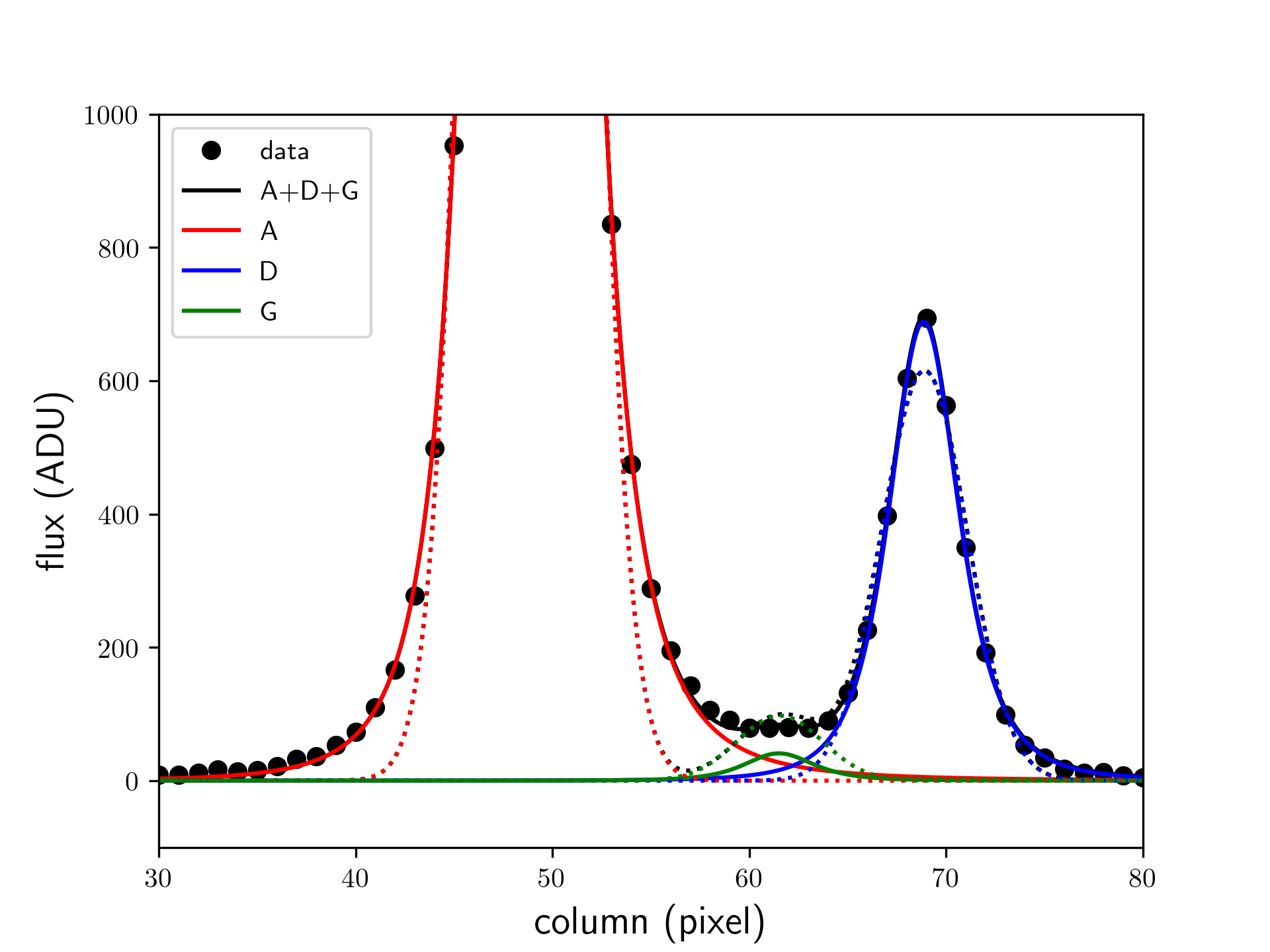
Figure 7: 1D flux distribution (along the slit) at $\sim$6800 Å. The black filled circles are the measured values, while the solid lines trace the global solution (black), and the individual contributions of A (red), D (blue), and G (green) using skewed Moffat profiles. Using Gaussian profiles, the global solution and the contribution of each source are also displayed as dashed lines.

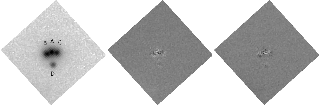
Figure 8: Left: 2D flux distribution in the $r$–band on 2018 August 13. Middle: Residual fluxes after subtracting only the best–fit model for the quasar images. Right: Residual fluxes after subtracting the full best–fit model. Residuals in the middle and right panels are linearly scaled between $-$3% and +3% of the maximum flux of A. The model consists of five components ABCDG and the fitting to data in the left panel is performed with IMFITFITS software (see main text).

Appendix B Extracting individual $r$–band fluxes of A, B, C, and D

As an example of the photometric fitting procedure, we first selected the $r$–band frame on 2018 August 13 (see Figure 3). The subframe of interest (containing the lens system) is shown in the left panel of Figure 8. Second, the 2D flux distribution in this subframe was modelled as four empirical PSFs (quasar images ABCD) plus a de Vaucouleurs profile convolved with the empirical PSF (main lensing galaxy G). The best–fit model from the IMFITFITS software package (McLeod et al., 1998) has a reduced $\chi^{2}$ of 1.28, which is a typical value when fitting system subframes at other epochs. The middle panel of Figure 8 displays the residual signal after subtracting the four quasar images. Regarding this panel, it is worth noting that the fluxes of ABCD are one or two orders of magnitude larger than the flux of G, and the galaxy is an extended source. Additionally, residuals correspond to a relatively short exposure with a 2m telescope. Hence, the light distribution in the middle panel is not dominated by emission from G. In the right panel of Figure 8, we also show the residual light after subtracting the full best–fit model (all sources). Pixels in this last subframe only contain the expected noisy signal.

It is worthy to mention that we analyse a crowded system using a well–tested photometric method. This worked quite well in other gravitational lens systems, since light curves from the IMFITFITS method basically agreed with those from alternative techniques, even using different telescopes (Alcalde et al., 2002; Ullán et al., 2006; Hainline et al., 2013; Gil-Merino et al., 2018). We also note that cross–talk between two close sources depends on the seeing, and sometimes it produces evident deviations (with respect to adjacent magnitudes) in the light curves of both sources (e.g., see discussion on systematic effects and the corresponding outliers in Sect. 4 of Goicoechea & Shalyapin, 2016). However, after removing data from frames with relatively poor seeing and two additional epochs producing evident outliers in the brightness record of the B image (see Section 3.1), our final light curves of PS J0147+4630 (catalog ) are not affected by significant systematic effects.

References

- Alcalde et al. (2002) Alcalde, D., Mediavilla, E., Moreau, O., et al. 2002, ApJ, 572, 729
- Berghea et al. (2017) Berghea, C. T., Nelson, G. J., Rusu, C. E., Keeton, C. R., & Dudik, R. P. 2017, ApJ, 844, A90
- Bessell (1999) Bessell, M. S. 1999, PASP, 111, 1426
- Bonvin et al. (2017) Bonvin, V., Courbin, F., Suyu, S. H., et al. 2017, MNRAS, 465, 4914
- Cappellari (2017) Cappellari, M. 2017, MNRAS, 466, 798
- Cappellari & Emsellem (2004) Cappellari, M., & Emsellem, E. 2004, PASP, 116, 138
- Chambers et al. (2016) Chambers, K. C., Magnier, E. A., Metcalfe, N., et al. 2016, eprint arXiv:1612.05560
- Eigenbrod et al. (2008a) Eigenbrod, A., Courbin, F., Sluse, D., Meylan, G., & Agol, E. 2008a, A&A, 480, 647
- Eigenbrod et al. (2008b) Eigenbrod, A., Courbin, F., Meylan, G., et al. 2008b, A&A, 490, 933
- Falcón-Barroso et al. (2011) Falcón-Barroso, J., Sánchez-Blázquez, P., Vazdekis, A., et al. 2011, A&A, 532, A95
- Fian et al. (2018) Fian, C., Mediavilla, E., Jiménez-Vicente, J., Muñoz, J. A., & Hanslmeier, A. 2018, ApJ, 869, A132
- Gil-Merino et al. (2018) Gil-Merino, R., Goicoechea, L. J., Shalyapin, V. N., & Oscoz, A. 2018, A&A, 616, A118
- Goicoechea & Shalyapin (2016) Goicoechea, L. J., & Shalyapin, V. N. 2016, A&A, 596, A77
- Hainline et al. (2013) Hainline, L. J., Morgan, C. W., MacLeod, C. L., et al. 2013, ApJ, 774, 69
- Howell (2006) Howell, S. B. 2006, Handbook of CCD Astronomy (Cambridge, Cambridge Univ. Press)
- Jackson (2015) Jackson, N. 2015, Living Rev. Relat., 18, 2
- Kochanek (2004) Kochanek, C. S. 2004, ApJ, 605, 58
- Lee (2017) Lee, C.-H. 2017, A&A, 605, L8
- Lee (2018) Lee, C.-H. 2018, MNRAS, 475, 3086
- McLeod et al. (1998) McLeod, B. A., Bernstein, G. M., Rieke, M. J., & Weedman, D. W. 1998, AJ, 115, 1377
- Moffat (1969) Moffat, A. F. J. 1969, A&A, 3, 455
- Morgan et al. (2018) Morgan, C. W., Hyer, G. E., Bonvin, V., et al. 2018, ApJ, 869, A106
- Pelt et al. (1996) Pelt, J., Kayser, R., Refsdal, S., & Schramm, T. 1996, A&A, 305, 97
- Rubin et al. (2018) Rubin, K. H. R., O’Meara, J. M., Cooksey, K. L., et al. 2018, ApJ, 859, A146
- Sánchez-Blázquez et al. (2006) Sánchez-Blázquez, P., Peletier, R. F., Jiménez-Vicente, J., et al. 2006, MNRAS, 371, 703
- Schönebeck et al. (2014) Schönebeck, F., Puzia, T. H., Pasquali, A., et al. 2014, A&A, 572, A13
- Shajib et al. (2019) Shajib, A. J., Birrer, S., Treu, T., et al. 2019, MNRAS, 483, 5649
- Shalyapin & Goicoechea (2017) Shalyapin, V. N., & Goicoechea, L. J. 2017, ApJ, 836, A14
- Shalyapin et al. (2002) Shalyapin, V. N., Goicoechea, L.J., Alcalde, D., et al. 2002, ApJ, 579, 127
- Sluse et al. (2007) Sluse, D., Claeskens, J. F., Hutsemékers, D., & Surdej, J. 2007, A&A, 468, 885
- Suyu et al. (2017) Suyu, S. H., Bonvin, V., Courbin, F., et al. 2017, MNRAS, 468, 2590
- Tody (1986) Tody, D. 1986, Proc. SPIE, 627, 733
- Tody (1993) Tody, D. 1993, in ASP Conf. Ser. 52, Astronomical Data Analysis Software and Systems II, ed. R. J. Hanisch, R. J. V. Brissenden, & Jeannette Barnes (San Francisco: ASP), 173
- Ullán et al. (2006) Ullán, A., Goicoechea, L. J., Zheleznyak, A. P., et al. 2006, A&A, 452, 25
- Woźniak et al. (2000) Woźniak, P. R., Alard, C., Udalski, A., et al. 2000, ApJ, 529, 88